Shifting water scarcities: irrigation alleviates agricultural green water deficits while increasing blue water scarcity

Agricultural areas often experience green water scarcity – the limitation of crop growth by soil moisture supplied through rainfall and snowmelt – due to e.g. unfavourable soil texture, high potential evapotranspiration rates, poor or inefficient crop management, and fluctuations in meteorological conditions. Driven by the growing effects of climate change and the rising water and food demands of an increasing world population, agricultural green water scarcity is becoming an increasingly important phenomenon. In this global modelling study, a plant-physiology based indicator of green water stress is applied, that quantifies the ratio between soil moisture limitation and atmospheric water demand on agricultural areas. Results show that currently (2015–2019 average) 44 % (686 Mha) of the global agricultural area is green water stressed. Hotspots are characterized by a high seasonal variability in stress conditions, and are mainly located in India and Pakistan, northern Sub-Saharan Africa, North Africa and southwestern Asia. Using an analogous blue water stress indicator – which relates human water use for households, industry and agriculture to available blue water resources – current irrigation is shown to alleviate plant water stress in agricultural areas by compensating for green water scarcity on 8 % (140 Mha) of the total agricultural area, but simultaneously increases the share of areas experiencing blue water stress by 6 % (96 Mha). This shift in water stress types highlights the importance of jointly considering the interconnected green and blue water resources and stresses in pathways towards sustainable water use in agriculture.

1 Introduction

Green water resources available to agriculture – the plant available soil moisture from rainfall and snow melt which sustains the growth of crops and pastures – account for 85 %–90 % of the water consumed by agriculture and are therefore of immense importance for securing global food production (Rost et al., 2008; Mialyk et al., 2024; Chukalla et al., 2025). Due to climate change and the intensification of agricultural practices in response to the higher food demand of the growing world population, green water scarcity (GWS), defined as the limitation of crop growth by insufficient green water resources, increases in many agricultural areas (He and Rosa, 2023; Liu et al., 2022a). In the future, even if the 1.5 °C climate mitigation target would be achieved, two thirds of the global rainfed cropland could be affected by GWS, posing a considerable threat to agricultural productivity and, consequently, global food security (He and Rosa, 2023).

Green water is especially indispensable on rainfed cropland, where it represents, together with capillary rise, the only water resource (Liu et al., 2022b). On irrigated cropland, blue water resources have the potential to compensate for plant water stress if GWS is high (Rosa et al., 2019). Therefore, green and blue water resources and limitations are not only strongly interconnected via the hydrological cycle but also through human interference (Gleeson et al., 2020). However, the practical implementation of irrigation often faces hindrances, primarily due to concurrent challenges such as blue water scarcity (BWS; Kummu et al., 2016; Mekonnen and Hoekstra, 2016) or a lack of irrigation infrastructure sometimes called economic water scarcity (IWMI, 2007; Rosa et al., 2020). Besides, irrigation systems are often inefficient, and a substantial portion of current global irrigation occurs in an unsustainable manner, impacting the maintenance of environmental flow requirements (EFRs) of aquatic ecosystems, depleting groundwater resources, and leading to severe water pollution (Falkenmark, 2013; Jägermeyr et al., 2017; Rosa et al., 2019; Dalin et al., 2019).

Blue water resources have long been the focus of water scarcity analyses since they are at the center of the competition between sectoral human water uses and EFRs (Kummu et al., 2016; Mekonnen and Hoekstra, 2016; Veldkamp et al., 2017) as well as human water stress under climate change and population growth (Heinke et al., 2019). Discussions about the central role, potential (increasing) limitation, and sustainable use of green water were long absent, as its availability was often taken for granted. While there are some integrated scarcity assessments, incorporating blue and green water resources (Rockström et al., 2009; Gerten et al., 2011; Rosa et al., 2020; Liu et al., 2022a, b, 2025), most of them simply overlay the different individual scarcities, not explicitly considering the interlinkages between them in a dynamic and process-based manner. For a consistent analysis, an approach is needed that (a) accounts for the balance of plant-available soil moisture and atmospheric moisture deficit, that determines GWS; (b) quantifies how the addition of blue water through irrigation ameliorates GWS; (c) traces how this irrigation may increase BWS; and (d) investigates whether sufficient blue water resources are in principle available to sustainably alleviate plant water stress under green water scarce conditions, e.g. not tapping into EFRs. The balance of plant-available soil moisture and atmospheric moisture deficit is particularly suitable for a GWS indicator, as it directly determines the stress level that plants are exposed to, limiting photosynthesis and growth. While Rosa et al. (2020) provide a quantitative, globally applicable approach to distinguish GWS and BWS, to our knowledge no study has quantified where and at what magnitude GWS has led to a shift towards higher BWS.

To address these research gaps, this study aims at analysing current spatial patterns and interlinkages of GWS and BWS related to agriculture, employing the LPJmL (Lund-Potsdam-Jena managed Land) dynamic global vegetation, crop and hydrological model (Schaphoff et al., 2018; von Bloh et al., 2018; Lutz et al., 2019; Wirth et al., 2024). Versions of this model have demonstrated capability to compute green-blue freshwater resources and limitations in coupling with natural and agricultural vegetation dynamics and in response to changes in climate, atmospheric CO₂ concentration, land cover/land use change, and crop and water management (Rost et al., 2008; Jägermeyr et al., 2015; Stenzel et al., 2019). A physiological GWS indicator is employed here, computed separately for each of the world's major crop types, taking into account the balance of soil moisture and atmospheric water demand, at daily time steps over the period 2015–2019, and on a global 0.5° grid. Based on this indicator, first, current GWS hotspots are identified. Second, BWS is calculated at daily timesteps for the same period and mapped on a monthly basis using an indicator which relates human blue water use (for households, industry and irrigated agriculture) to available blue water. Third, it is traced where and to what degree irrigation compensates for GWS but at the same time increases BWS. Finally, the extent to which local blue water resources would be sufficient to buffer GWS without ecologically unsustainable appropriation of EFRs is quantified.

2 Methods

2.1 The Dynamic Global Vegetation Model LPJmL

LPJmL simulates the growth and productivity of natural and agricultural vegetation with the coupled water, energy, nitrogen, and carbon pools and fluxes (for detailed model descriptions see Bondeau et al., 2007; Schaphoff et al., 2018; von Bloh et al., 2018). It further captures the spatial and temporal variations of these processes in response to climatic conditions and human interventions such as crop management and irrigation (Jägermeyr et al., 2015, 2017; Lutz et al., 2019; Herzfeld et al., 2021; Porwollik et al., 2022; Minoli et al., 2019, 2022). Simulations are performed at a spatial resolution of 0.5° (further specifying fractions of each grid cell assigned to different crop, irrigation and pasture systems, the remainder is simulated as dynamic natural vegetation), at daily time steps. Natural vegetation is represented by 11 plant functional types (PFTs) and agricultural vegetation by 12 crop functional types (CFTs) and grassland/pastures. In this study, CFTs are the focus, including: temperate cereals, rice, maize, tropical cereals, pulses, temperate roots, tropical roots, sunflower, soybean, groundnut, rapeseed, sugar cane, in addition to an “others” category, which aggregates all crops not parameterised specifically as CFTs (see Schaphoff et al., 2018). The 12 parameterised CFTs cover ≈ 60 % of the global agricultural area while “others” (including also perennial crops – like coffee, cocoa and tea) cover ≈ 40 % (see the Supplement for more details on the model setup). CFTs are considered to be either rainfed or irrigated, prescribed by a land-use input dataset (see below).

Each CFT is simulated with its own soil bucket, so that the irrigation water requirement is crop-specific and the green water supply not influenced by the other plants. Daily net irrigation is determined for each CFT based on the soil water deficit, the CFT-specific water demand given by atmospheric moisture deficit, and the efficiency of the specific irrigation systems (Jägermeyr et al., 2015 (Table 5); Schaphoff et al., 2018). Grid and crop specific irrigation systems (sprinkler, furrow and drip irrigation) are prescribed (Jägermeyr et al., 2015). The dataset used is derived from suitability-based decision rules and a structured algorithm that ensures consistency with observed national irrigation system distributions (more details can be found in the Supplement). Irrigation is applied to the field if CFT-specific water stress occurs (water supply being lower than water demand) and soil moisture falls below a CFT-specific irrigation threshold. LPJmL assumes withdrawal of irrigation water from available blue water, e.g. rivers, lakes and reservoirs, including from neighboring upstream cells if the computed blue water availability of the cell where the demand occurs is not sufficient (accounting for local water diversion schemes and possible mismatches between the input datasets on river topology and irrigated areas).

LPJmL employs an implemented routing module which represents upstream–downstream relations through the predefined river network, where discharge flows between grid cells with a constant flow velocity and via cascaded linear reservoirs (Schaphoff et al., 2018). Water deficits are calculated locally in each cell, but propagate downstream because reduced outflow from an upstream cell decreases available discharge for all downstream cells. Return flows from irrigation losses are assumed to percolate into the soil and subsequently contribute to surface runoff, which is added to the local surface water and routed downstream. Reservoirs further modify these interactions by storing, buffering, and releasing water according to their operating rules, thereby altering both local and downstream water availability.

2.2 Simulation protocol and model runs

In this study, LPJmL version 5.9.25 was run with forcing of historical climate and land use for the period 1901–2019, preceded by a 3500-year spin-up period in order to bring the PFT distribution and carbon and nitrogen pools into a dynamic prehistoric equilibrium and a subsequent land use spin-up featuring historical land-use patterns since 1500 (for further information, see Fig. S1 in the Supplement). Daily climate forcing data were taken from the GSWP-W5E5 dataset (Lange et al., 2021; see Table 1), with the first 30 years being randomly recycled for the simulation years before 1901. Land-use input obtained from the LandInG 1.0 toolbox (Ostberg et al., 2023) is used by the model to simulate each CFTs' growing period and seasonal phenology, as well as crop production and yield. The LandInG toolbox derives rainfed and irrigated crop maps from a combination of country-level and gridded datasets, including FAOSTAT, MIRCA2000, AQUASTAT, MON, RAM, and HYDE (see Ostberg et al., 2023, for references, also for further specifics such as the soil type database used). Country-level datasets provide information on crop-specific harvested areas and changes over time, while gridded datasets provide spatial detail or temporal dynamics but may lack crop-specific information. LandInG integrates these sources to create a harmonized, gridded dataset at 0.5 resolution, covering 1500–2017, by disaggregating country-level data to grid cells and resolving inconsistencies between datasets. This processing allows the toolbox to capture spatiotemporal changes in rainfed and irrigated crop distributions while maintaining consistency with crop-specific and irrigation-specific information available at coarser, e.g. national, resolution. We furthermore use the GGCMI Phase 3 crop calendar described in Jägermeyr et al. (2021) which is static in sowing dates and crop variety parameters, but the length of the growing season is variable according to temperature variations. Multiple cropping is not represented in LPJmL. In our model setup, the root zone is kept static over the growing season. The soil column is represented by six layers, of which five are hydrologically active (with depths of 0.2, 0.3, 0.5, 1.0, and 1.0 m, for more detail see Schaphoff et al., 2018).

Table 1 Main input data for LPJmL simulations.

Monthly water use input for the sectors of domestic use, electricity generation (cooling of thermal power plants), livestock, mining and manufacturing is taken from Huang et al. (2018). Availability of green water (and potentially added blue irrigation water) is computed separately for each CFT, based on their specific soil water budget. While CFTs do not compete for green water, irrigation water is allocated based on local blue water availability within each grid cell (river inflow excluding upstream water use, as well as reservoirs and lakes). Irrigation is assumed to occur to the extent it can be met by this daily, grid-cell specific blue water availability (“limited irrigation scenario” ILIM, not additionally including long-distance transfers or fossil groundwater; see Rost et al., 2008). To isolate effects of irrigation and thereby derive the climate-driven effect on GWS, a “no-irrigation scenario” is also analysed (INO, performed for 1990–2019) that considers all agricultural land to be rainfed. For better comparability of irrigated CFTs in INO and ILIM, the growing seasons of the concerned CFTs in INO are adjusted so that they retain their actual growing season length (as in ILIM) and do not adapt to the rainfed growing season. Furthermore, a groundwater buffer represents subsurface water storage and sustains baseflow during dry periods by releasing water at a fixed rate of 0.01 d⁻¹ relative to its volume (based on Döll et al., 2003), simulating a simplified renewable groundwater discharge. While shallow groundwater is implicitly included in the baseflow scheme, the groundwater reservoir operates independently from soil moisture processes; thus, capillary rise and direct renewable groundwater inflows are not explicitly represented. Instead, these inflows are implicitly captured through drainage from the lowest soil layer contributing to river discharge. This groundwater buffer thus influences the discharge (see Fig. S2 in the Supplement), but is not actively used as a source for irrigation withdrawals.

2.3 Green water stress

The GWS indicator (see Fig. 1) is defined as the unitless ratio of plant-available soil water supply (S) and atmospheric demand (D), per CFT and grid cell on a monthly basis (derived from the average of daily values):

$$\begin{array}{}\text{(1)}& \mathrm{GWS}=\mathrm{1}-{\displaystyle \frac{S}{D}}\end{array}$$

The plant-available soil water supply (in mm) is calculated as follows:

$$\begin{array}{}\text{(2)}& S=E_{\max }\cdot w_{\mathrm{r}},\end{array}$$

where E_max is the maximum daily transpiration rate for crops (8 mm d⁻¹, based on Fader et al., 2010), and w_r is the relative soil moisture of the root zone, scaled between 0 (no green or blue water available) and 1 (fully saturated).

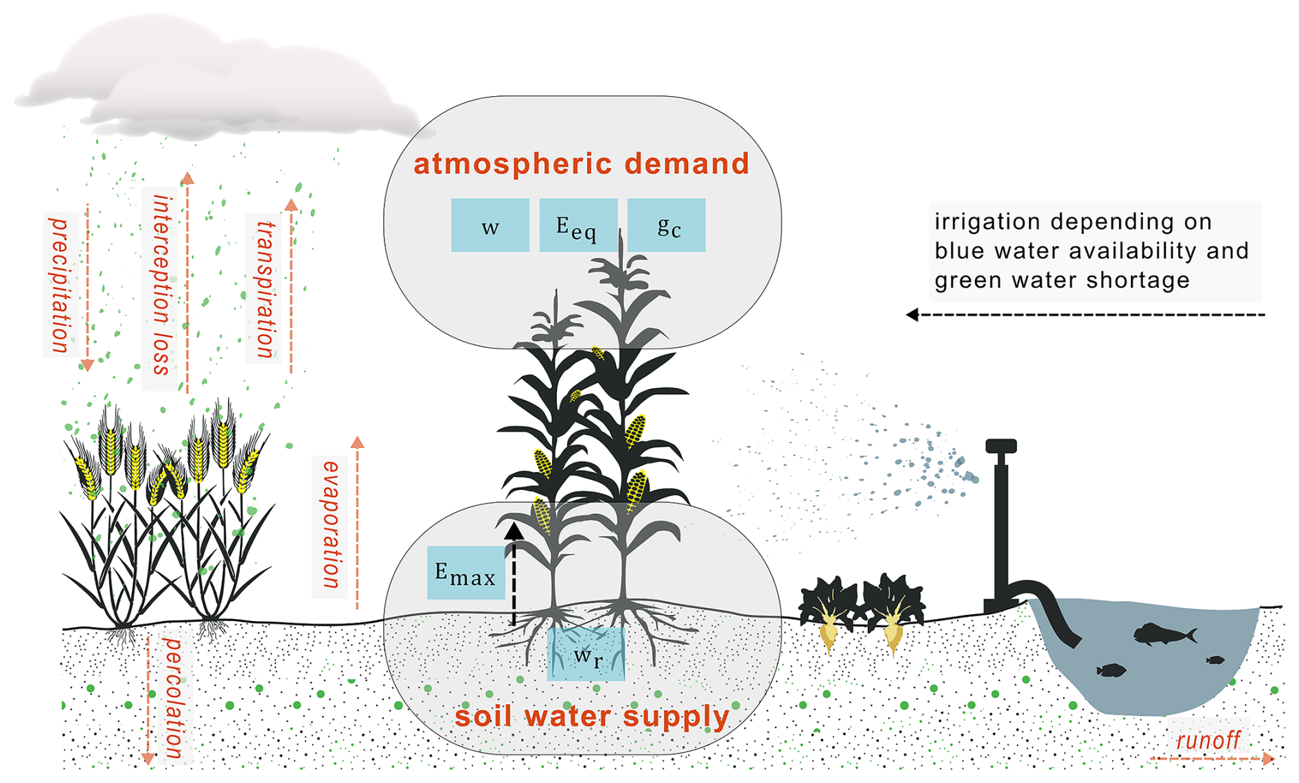
Figure 1 Schematic overview of basic processes considered in the calculation of the green water scarcity indicator. See text/equations for abbreviations.

The atmospheric demand (in mm) represents the daily “optimal” transpiration of a given CFT (unconstrained by soil moisture limitation) and is defined according to the following hyperbolic function:

$$\begin{array}{}\text{(3)}& D={\displaystyle \frac{\left(\mathrm{1}-w\right)\cdot E_{\mathrm{eq}}\cdot {\mathit{\alpha }}_m}{\left(\mathrm{1}+\frac{g_m}{g_{\mathrm{c}}}\right)}},\end{array}$$

where w is the amount of energy used to vaporize the intercepted water in the vegetation canopy (fraction of the day the canopy is wet); E_eq is the equilibrium evapotranspiration; α_m is the Priestley-Taylor coefficient (1.391; based on Priestley and Taylor, 1972); g_m presents a scaling factor 3.26 (average based on Huntingford and Monteith, 1998) and g_c the potential canopy conductance that would occur if soil moisture was not limiting.

The GWS indicator ranges from 0 to 1, with 1 indicating complete water stress, and 0 representing an unstressed condition where soils can provide adequate water to meet D. If S>D, we set S=D, because plants cannot take up more water than their transpiration demand allows. If S<D, the plants' physiological activities decline, impacting their transpiration, biomass production, as well as carbon sequestration (see details in Gerten et al., 2005, 2007, who used a similar indicator for natural vegetation).

Monthly GWS is calculated for rainfed and irrigated CFTs based on the ratio of monthly sums of demand and supply, considering only days when the crop is actively growing. Days without any water demand are omitted from the aggregation. To calculate the average GWS for a grid cell, GWS was weighted by the annual CFT-specific area fraction and normalized by the sum of all CFT fractions. Detailed maps of CFT-specific GWS can be found in the Supplement (see Fig. S3).

Instead of using one general GWS threshold as in other studies (Rosa et al., 2020; He and Rosa, 2023), we calculated CFT-specific thresholds based on yield responses modeled with LPJmL. We conducted two LPJmL simulations, both implemented with unrestricted nitrogen availability and nitrogen-insensitive maintenance respiration to exclude nitrogen limitation. In the first scenario (INO_threshold), all cropland is treated as rainfed. In the second scenario (IALL_threshold), all agricultural areas are assumed to be fully irrigated and therefore do not experience GWS, representing an optimal scenario. By comparing the IALL_threshold yields with those of the INO_threshold run, we calculated the percentage yield decline from IALL_threshold to INO_threshold attributable to GWS. For each CFT, we generated scatterplots illustrating how increasing GWS values correspond to increasing yield declines (see Fig. S4). This relationship was modeled with a logistic regression for each CFT. From these fitted models, we derived CFT-specific levels at which yields decline by 10 %, 20 %, 30 %, etc. (in gC m⁻²) due to GWS.

Based on these yield declines, we developed GWS categories in sequential steps of 20 % yield decline (0 %–20 % = low GWS, 20 %–40 % = moderate GWS, 40 %–60 % = high GWS, 60 %–80 % = severe GWS and 80 %–100 % = extreme GWS), in order to show a graduality in the GWS exposure (see Sect. 3.2).

2.4 Blue water stress

Similar to the GWS, the BWS indicator presents a local water use to availability ratio and is computed for each grid cell on a monthly basis (see Eq. 4). It compares consumptive water use for households, industry and livestock (WU_HIL, converted to m³ month⁻¹) and consumptive water use for irrigation (WU_irr, converted to m³ month⁻¹) to local water availability, which is calculated from the available river discharge of a grid cell (Q):

$$\begin{array}{}\text{(4)}& \mathrm{BWS}={\displaystyle \frac{{\mathrm{WU}}_{\mathrm{HIL}}+{\mathrm{WU}}_{\mathrm{irr}}}{\mathrm{local}\mathrm{water}\mathrm{availability}}}\end{array}$$

WU_HIL are inputs taken from Huang et al. (2018). This dataset was created by spatially and temporally downscaling national (and US state-level) sectoral water-withdrawal estimates from AQUASTAT and USGS, providing a monthly 0.5° gridded dataset for the period 1971–2010. In this study, values after 2010 are held constant. We use data from the following sectors from this dataset: domestic, electricity generation (cooling of thermal power plants), mining, manufacturing and livestock.

WU_irr was calculated with LPJmL as follows:

$$\begin{array}{}\text{(5)}& {\mathrm{WU}}_{\mathrm{irr}}={\mathrm{WD}}_{\mathrm{irr}}+E_{\mathrm{conv}}-\mathrm{RF},\end{array}$$

where WD_irr presents applied irrigation water (mm month⁻¹), E_conv evaporative conveyance loss (mm month⁻¹) and RF water return flow (mm month⁻¹).

For calculating BWS in this study, only local water availability within a grid cell is considered. This is a simplification, since LPJmL can draw on transboundary water resources from upstream neighboring cells and/or reservoirs for irrigation. However, LPJmL does not provide output that partitions consumptive water use by source (local versus these external supplies); therefore, we did not include consumptive use from external sources in this analysis. Renewable groundwater inflows are implicitly captured through drainage from the lowest soil layer contributing to river discharge (see Sect. 2.2).

Contrarily to the GWS indicator, the BWS indicator thus not solely considers water use for agriculture but from other sectors as well (which however do not affect the difference in BWS between the ILIM and INO simulations as they are always prioritized). A higher BWS indicates greater stress, reflecting the extent to which total human water demand approaches or exceeds the renewable freshwater supply. Blue water stress is assumed to be moderate (high) in cells where the yearly mean BWS is >0.2 (>0.4) (Raskin et al., 1997; Vörösmarty et al., 2000).

2.5 Sustainable blue water use

EFRs are a method to quantify aquatic ecosystem water needs. We define blue water use in agriculture as unsustainable water overuse if it leads to transgressions of EFRs, which implies that withdrawals reduce river flows below levels needed to maintain ecological integrity and thereby contribute to biodiversity loss. We calculated EFRs for every grid cell on a monthly level using the Variable Monthly Flow method, which accounts for the intraannual variability of river flows and separates the flow regime into high, intermediate, and low-flow months (Pastor et al., 2014). We calculate the EFRs based on the discharge of a baseline run for the period 2015–2019 (thereby not taking into account climate change effects), that features an active reservoir network but excludes any water abstractions for irrigation or other human purposes. Water overuse (O) was calculated for each grid cell as:

$$\begin{array}{}\text{(6)}& \begin{array}{rl}O& ={\mathrm{WU}}_{\mathrm{irr}}-\mathrm{sustainable}\mathrm{water}\mathrm{availability},\mathrm{set}\mathrm{to}\mathrm{0}\\ & \mathrm{if}<\mathrm{0}\left(=\mathrm{no}\mathrm{overuse}\right)\end{array}\end{array}$$

Sustainable water availability in a grid cell is here defined as the discharge available for irrigation minus the EFRs, ensuring that other water uses have already been accounted for, with values truncated at zero where EFRs exceed the available discharge (e.g. due to other water uses).

The resulting water overuse values were then summed up over all agricultural grid cells to derive a global estimate. Upstream–downstream relationships among cells, which are particularly crucial for accurately computing water overuse, are represented through a routing module (Schaphoff et al., 2018).

3 Results

3.1 Global hotspots of green water stress

To exclude the ameliorating impact of irrigation, average GWS of all CFTs was assessed in the INO scenario that assumes all agricultural areas to be rainfed for the time period 2015–2019 (Fig. 2a). In this section, we only describe the averaged GWS patterns, GWS classifications based on yields follow in Sect. 3.2. Major GWS hotspots with values close to 1 – in the absence of irrigation – are found to be located in southwestern Asia and North Africa, particularly in Iran, Afghanistan, Pakistan, Egypt and on the Arabian Peninsula. Other, albeit less green water stressed regions with values >0.6, are located in northern Sub-Saharan Africa, e.g. Sudan, Somalia and Niger, and southern Africa where local communities are highly dependent on rainfed agriculture. Also, regions in Mongolia and Kazakhstan, eastern Australia, South America, Mexico and the USA experience values of GWS >0.6. Regions with little GWS (annual average <0.2) even without irrigation include large areas of Europe, parts of eastern China, rainforest regions, and parts of the US. In these regions, soil water supply is able to meet atmospheric water demand in most months of a year.

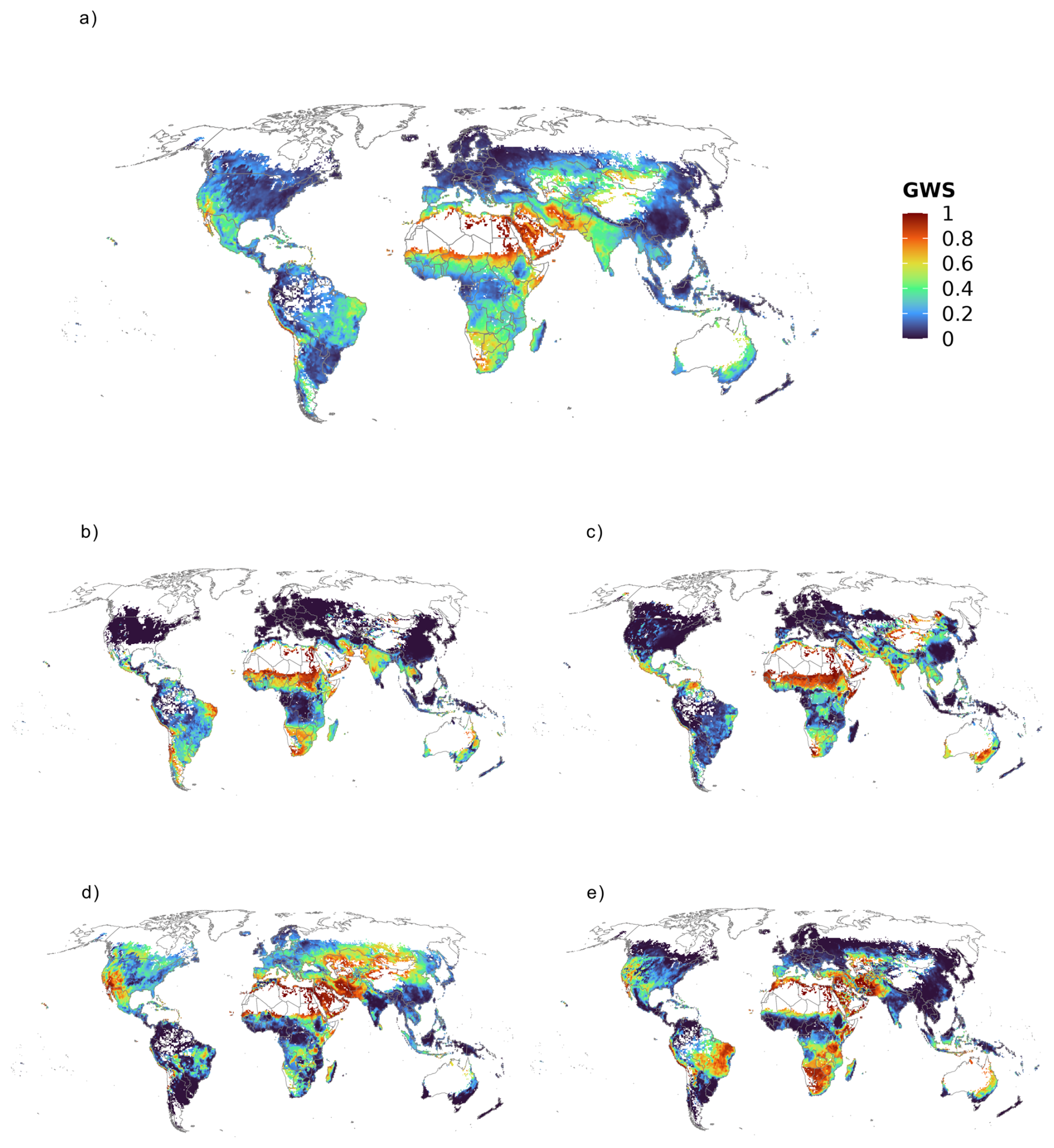
Figure 2 LPJmL-simulated GWS in the absence of irrigation (INO scenario) across crop functional types for the time period 2015–2019 as a) yearly average and b)–e) seasonal averages: b) December–February, c) March–May, d) June–August and e) September–November. White areas indicate that no crops are growing in this period. The legend applies for all panels.

The green water stress patterns show a high seasonal variability over the year due to changing weather conditions but also season-specific growing seasons (Fig. 2b–e). Europe and North America do experience less (or even no) GWS during the winter months since the water demand of the crops grown during that time is very low (Fig. 2b). During the summer months (Fig. 2d), however, especially southern regions in Europe and the western US show average GWS values >0.4. Large regions in Brazil become GWS hotspots from June to November, when GWS values are especially high for pulses, rapeseed and sugarcane (Fig. 2d–e). India, by contrast, is no GWS hotspot from June to November (Fig. 2d–e), when most crops are grown. However, temperate cereals, pulses, oil crops, and sugarcane, which are cultivated in the dry winter monsoon season, do exhibit higher GWS values. Besides the overall regional and seasonal features, the simulated GWS patterns also show differences in GWS between the individual years (see Fig. S5 for seasonal maps of the years 2017, 2018 and 2019). While the global mean GWS remained relatively stable during this period (ranging from 0.233 to 0.237), significant regional variations occurred. For instance, the drought in large parts of Europe in 2018 is well captured, as are the generally very wet conditions in 2017 there (for a comparison see Fig. S6).

3.2 Green water stress thresholds based on yield declines

In this study, we defined CFT-specific GWS categories based on yield declines, which were calculated from the difference of an optimal yield scenario (without water or nitrogen limitation) and a scenario without nitrogen but with water limitation (all areas considered as rainfed). This allows a meaningful link between GWS values and their impacts on agriculture. Figure 3a shows the results for five exemplary CFTs. Our findings indicate large differences in the CFT yield responses with regard to GWS: While some CFTs (e.g. oil crops soybean) experience a 20 % yield decline at a GWS value of approximately 0.2 under rainfed conditions, other crops (e.g. oil crops rapeseed) experience a yield decline of 40 % under similar GWS conditions. While oil crops sunflower show an 80 % yield decline at a GWS value of 0.46, sugarcane only experiences a similar yield decline at a GWS value around 0.6. Scatterplots and tables with GWS thresholds for all CFTs can be found in the Supplement (see Fig. S4 and Table S1).

Figure 3b shows the green water stressed areas for all individual CFTs in the INO run (average 2015–2019), based on the described thresholds. The most green water stressed CFT under rainfed conditions is oil crops sunflower, here, 92 % of the area experiences GWS, followed by sugarcane (86 %) and pulses (82 %). For a detailed summary of all CFTs and their GWS categories, see Table S2.

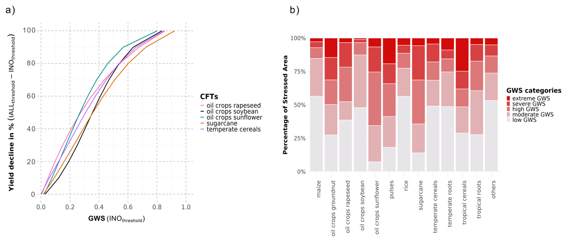
Figure 3 Green water stress thresholds and CFT-specific green water stress, where a) shows thresholds (relationship between GWS on rainfed areas and yield decline) for five selected CFTs and b) shows the CFT-specific area stressed for the no irrigation (INO) scenario.

3.3 Irrigation-induced shifts from green to blue water stress

While the above analysis assumed all agricultural areas to be rainfed (INO), we here compare the INO and the limited irrigation (ILIM) scenarios to firstly quantify the GWS-compensating effect of irrigation and secondly the degree to which this irrigation increases BWS.

Table 2 shows that 52 % (824 Mha) of all global cropland is green water stressed (>20 % of potential harvest are lost due to GWS) in the INO scenario, with 23 % of the area (360 Mha) experiencing moderate GWS (20 %–40 % harvest loss), 14 % (291 Mha) high GWS (40 %–60 % harvest loss), 9 % (148 Mha) severe GWS (60 %–80 % harvest loss) and 6 % (99 Mha) extreme GWS (>80 % harvest loss). With irrigation (ILIM scenario) the area that experiences GWS decreases to 44 % (687 Mha), where 20 % are classified as moderately, 12 % as highly, 7 % as severely and 5 % as extremely stressed. This means that irrigation compensates for GWS on 8 % of the global cropland area (140 Mha), effectively reducing the stress plants experience.

Table 2 Calculation of the extent of water stressed areas.

Table 3 Calculations of associated global water volumes.

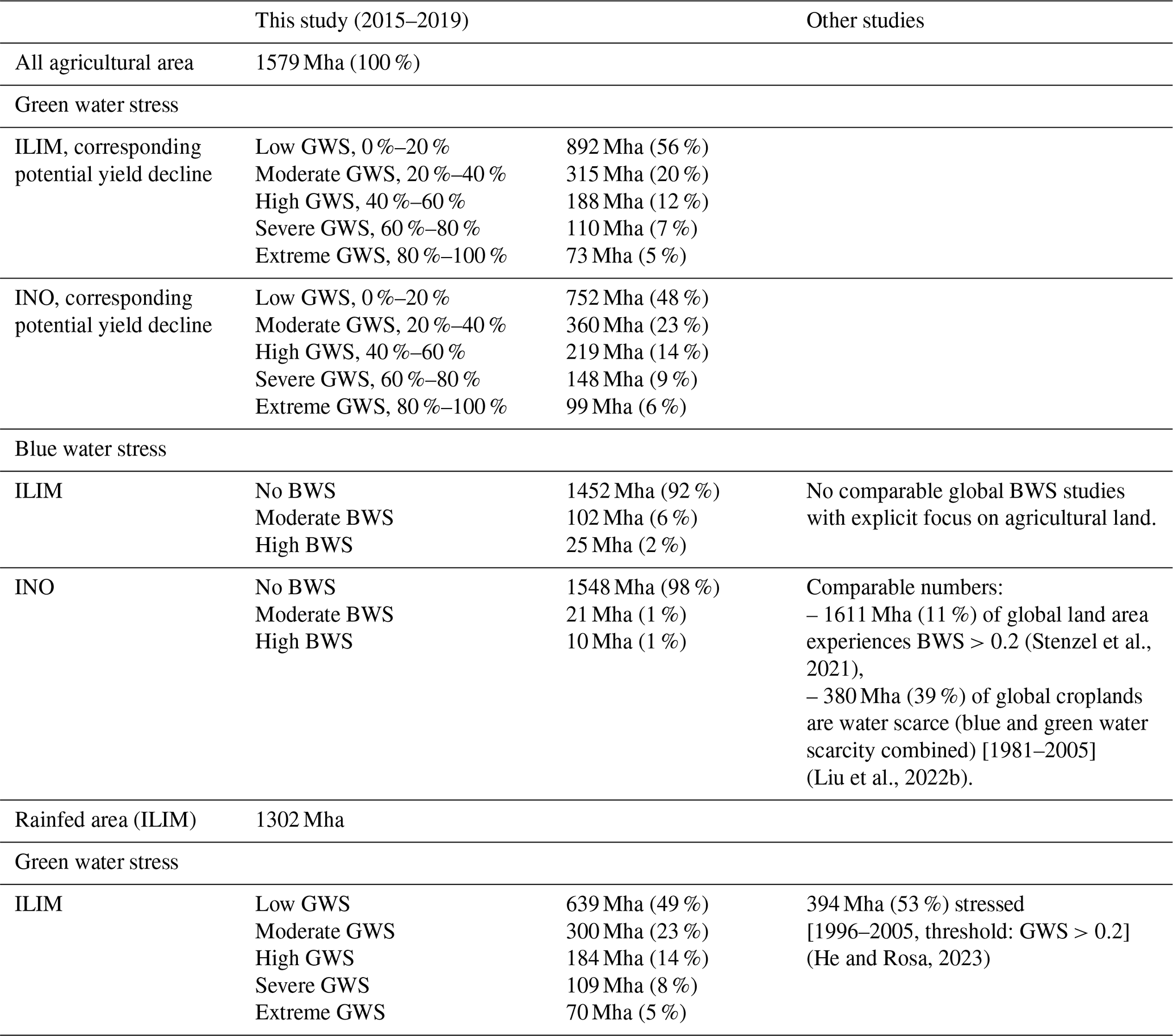
Figure 4 illustrates the difference of GWS between the INO and ILIM scenario, averaged over the time period 2015–2019. According to expectation, irrigation significantly ameliorates GWS in many regions, for example in Southwest Asia, India, Southern Africa and Peru. Figure 5a shows the simulated spatial patterns of combined GWS and BWS under the ILIM scenario. Figure 5b focuses on irrigated cells and highlights that in the INO scenario, only 46 % of the agricultural area experience low GWS (<20 % harvest loss), but with irrigation (ILIM), this number increased to 66 % (see Table S3). Correspondingly, the area in irrigated cells facing moderate GWS drops from 23 % without irrigation to 16 % with irrigation, for high GWS from 13 % to 9 %, for severe GWS from 11 % to 5 % and for extreme GWS from 7 % to 4 %. In our analysis, irrigated cells comprise both irrigated and rainfed agricultural areas. To ensure consistency with the BWS indicator, analyses were conducted at the grid-cell level. Consequently, even in irrigated cells, substantial portions of the area experience GWS under the ILIM scenario. Figure 5c illustrates the net change in green water stressed area per CFT between the ILIM and INO scenarios as a percentage of total agricultural area, highlighting a shift where acreage decreases in high-stress categories and increases in the low-stress category. Irrigation has a positive influence on green water stress of all crops, but influences sugarcane the most: Here, the area categorized as low GWS increases by around 35 % due to irrigation.

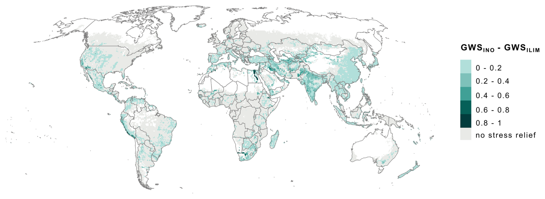
Figure 4 Green water stress relief due to irrigation. LPJmL-simulated difference between values of GWS in the INO and ILIM simulations, averaged for the time period 2015–2019.

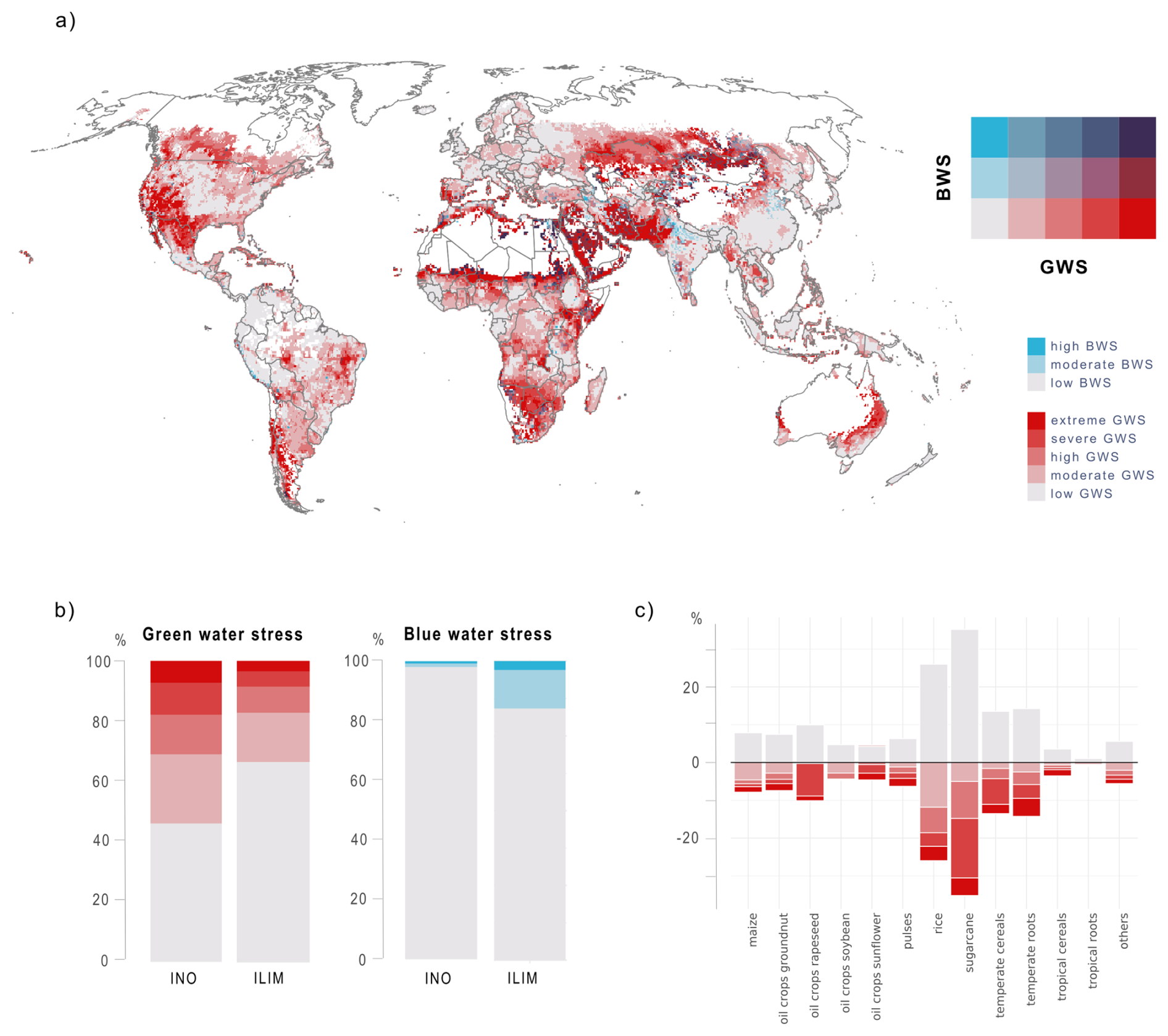
Figure 5 Combined water stresses: a) simulated spatial pattern of combined GWS and BWS under ILIM, averaged over the period 2015–2019, since a single grid cell can contain multiple GWS categories (due to multiple CFTs), only the dominant category is displayed here, b) shifts in water stresses in agricultural areas in cells with irrigation from the INO to the ILIM scenario for GWS and BWS, and c) net change in green water stressed area per CFT between the ILIM and INO scenarios as a percentage of total agricultural area of the respective CFT, averaged over the period 2015–2019. The legend showing GWS and BWS categories applies for all panels, where grey to blue shades along the y axis indicate increasing BWS and grey to red shades along the x axis indicate increasing GWS; for panel a), the diagonal line from light grey in the lower left to dark violet in the upper right indicates increasing combined BWS and GWS.

Figure 5a furthermore shows that regions mainly experiencing BWS are in India, China, Southwest Asia, parts of the US, southern Africa and the Mediterranean. In the ILIM run, we find that 6 % (102 Mha) of all global agricultural areas (rainfed and irrigated) experience moderate (BWS >0.2) and 2 % (25 Mha) experience high (BWS >0.4) blue water stress (see Table 2). Comparing these results with the INO scenario (1 % for both cases) confirms that the main reason for BWS is irrigation water use, as detailed in the following based on model results shown in Fig. 4a (see Fig. S7 for only BWS). A detailed look at agricultural areas in cells with irrigation (Fig. 5b) highlights again that the GWS-compensating effect leads to a shift from GWS to BWS there. In the INO scenario, only 1 % of the agricultural area in cells with irrigation experience moderate as well as high BWS, respectively (due to water extraction for industrial and domestic purposes), but with irrigation in the ILIM scenario, these shares rise to 13 % and 3 %, respectively (see Table S4). These shifts happen mainly in regions like India, Iran, Southern Africa but also Türkiye or Spain.

3.4 Sustainable use of blue water resources

In a final step, it is analysed whether sufficient blue water resources are available to sustainably alleviate plant water stress (i.e. decreasing the GWS indicator value to near 0) – which is a hypothetical scenario as in reality EFRs are often neglected. Figure 5a already shows that some areas that experience both GWS and BWS are located in southwestern Asia, Pakistan, Afghanistan, Somalia, Brazil, Mexico and the US. The simultaneous stress of both green and blue water already indicates that GWS is often mitigated at the expense of blue water resources.

We find that during the study period, on average 173 km³ yr⁻¹ of blue water resources have been added non-sustainably, leading to the transgression of EFRs (see Fig. 6). This overuse accounts for 12 % of the total irrigation water consumption (around 1217 km³ yr⁻¹), with particularly high volumes in India and China.

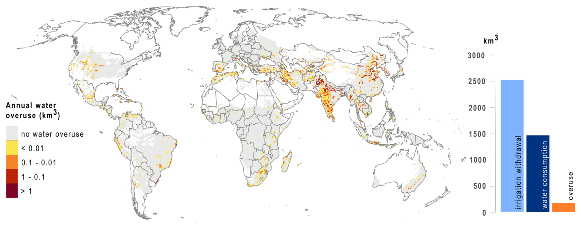
Figure 6 Annual unsustainable water overuse on agricultural areas (km³, average 2015–2019). The bars to the right indicate the globally aggregated volumes.

4 Discussion

4.1 Green water stress indicator and hotspots

This study identifies current hotspots of GWS in agricultural regions on an annual and seasonal scale for the time period 2015–2019. The GWS indicator used focuses not solely on soil moisture, but on CFT-specific water demand and water supply and therefore may reflect low water stress even under low soil moisture conditions, as long as atmospheric evaporative demand is also low. In general, the GWS hotspots identified here are in line with spatial patterns of earlier studies, even though regional differences exist. Comparing the results of our GWS indicator to He and Rosa (2023), who computed GWS as the ratio of irrigation water requirements and crop water requirements for the baseline period 1996–2005 on rainfed areas (see Fig. S8), illustrates that their study shows more extreme GWS, as e.g. in the western USA or Europe. While He and Rosa (2023) find a similar share of green water stressed rainfed area (53 % vs. 51 % in our assessment), the absolute areas under green water stressed conditions substantially differ (see Table 2). This may be attributed to a much lower assumed rainfed area in He and Rosa (2023) (1302 Mha in our study vs. 555 Mha in He and Rosa, 2023). The much lower rainfed area in He and Rosa is probably due to the exclusion of all cells (5 arcmin resolution) with more than 5 % of area equipped for irrigation. He and Rosa further used a different, very common approach, to define GWS: An area is considered green water stressed if the ratio of irrigation water requirements and crop water requirements >0.2. This approach does not enable the identification of crop-specific GWS thresholds. In our study, regions are characterized as green-water scarce when GWS leads to yield reductions >20 % relative to a scenario without water limitation. With this approach, we are able to define CFT-specific GWS thresholds based on the relationship between green water and crop yields. In contrast to the frequently used actual to potential evapotranspiration (AET $/$ PET) ratio, which rather represents an average situation across land systems, our GWS indicator shows that even though indicator values vary, spatial patterns remain similar (see Fig. S9).

In LPJmL, multiple cycles of the same crop or different crops in one year are not implemented. The inclusion of multiple cropping would however provide a more accurate representation of agricultural practices in regions with multiple harvests per year and also be essential for properly assessing the benefits of irrigation (Waha et al., 2025). Previous work (e.g. Biemans et al., 2016) has shown that enabling multi-cropping in LPJmL led to better seasonal estimates of irrigation-water demand. We therefore likely underestimate irrigation water supply and thus the alleviation of GWS in this study. A second underestimation might arise from the ILIM setting of this study, where biases in LPJmL in reproducing the seasonal cycle of discharge might lead to artificial mismatches in water supply and irrigation water demand.

4.2 Interlinkages between green and blue water stress

Combining green and blue water stresses revealed that they are strongly interlinked through irrigation. While irrigation increased the extent of agricultural areas experiencing low GWS by 8 %, it thereby led to an increase in areas experiencing moderate BWS as well as high BWS by 6 %. However, the shift in water stresses from green to blue is recognized to rely on the definition and simulation of the water stress indicators (see above for GWS), as well as irrigation assumptions in LPJmL.

The BWS indicator used in this analysis has been applied in numerous studies (Vörösmarty et al., 2000; Smakhtin et al., 2004; Kummu et al., 2016). In its original version, it is meant to reflect local availability by accounting for available water from river discharge only. It does not assume the sharing, transfer or trade of water. Irrigation in LPJmL, however, not only relies on local river discharge but also on water withdrawals from reservoirs and withdrawals from upstream neighboring cells. These additional water sources were not included in the calculation of water availability for BWS. While LPJmL provides information on irrigation withdrawals, it does not track consumptive water use associated with upstream withdrawals or reservoirs. Estimating consumptive water use is therefore not easy, as withdrawals occur in different grid cells than conveyance losses and return flows. Consequently, the chosen approach likely leads to an overestimation of BWS, as it is based solely on local water availability; nevertheless, given the structure and limitations of LPJmL, this represents the most consistent and feasible approximation. For the calculation of the BWS, it would be beneficial to consider not only water available in the given grid cell but also external water inflows. These could be water withdrawals from upstream cells or long-distance water transfers – such as those via irrigation canals – which often play a significant role in highly irrigated regions.

The results of this study are further influenced by regional factors of irrigation, such as different water use efficiencies, the precise location of irrigation systems or the type of irrigation applied. These variables have a strong influence on BWS (Jägermeyr et al., 2015), addressing their uncertainties is however beyond the scope of this study. Further, LPJmL does not include fossil groundwater resources which are a main source of irrigation water extraction in many regions. This also has implications for the sustainable use of blue water resources since in reality 20 % of irrigation relies on non-sustainable groundwater withdrawals (Dalin et al., 2019), which in our simulations might be discarded because no water is available or replaced by sustainable surface water withdrawals (not leading to EF transgressions). For a holistic picture, it would be valuable to include information on groundwater volumes and abstractions.

4.3 Implications for water management and global food security

We find that 173 km³ yr⁻¹ of blue water resources used violate EFRs. The EFRs were calculated in a post-process manner using the VMF method (Pastor et al., 2014), however, further analyses could apply several EFR estimation methods and compare their results accordingly (as in Jägermeyr et al., 2017). In this study, we also do not discuss the degree to which GWS alleviation would be reduced if EFRs would be preserved internally in LPJmL. It would be furthermore beneficial to also include other sustainability criteria than the EFRs in order to account for sustainable blue water management. Compared to recent studies on unsustainable water use by Rosa and Sangiorgio (2025) as well as Citrini et al. (2025) which identified unsustainable irrigation water consumption (or global “water gap”) to be 458 km³ yr ⁻¹ (2001–2010), our results indicate a lower overuse volume. This difference might occur due to the different models and baselines used as well as our restriction of blue water availability to surface water resources while Citrini et al. also include seasonally renewable groundwater. Comparing the spatial patterns of water overuse in our study with the results of Rosa and Sangiorgio (2025) reveals very similar distributions: Unsustainable water use mainly occurs in India (especially northern regions), Western China, West Asia, Portugal and Spain, and across the western USA and Mexico.

In this study, irrigation was shown to have the dual effect of compensating for GWS while simultaneously increasing BWS. In practice, this situation could be avoided by adopting more sustainable crop and water management strategies (Elsayed et al., 2025), such as enhanced green water management options, like mulching or conservation tillage (Jägermeyr et al., 2017; Gerten et al., 2020). More effective irrigation systems, for example, could limit this negative effect – further analyses could model this potential by e.g. assuming drip irrigation systems everywhere as in Jägermeyr et al. (2015). Also, water losses towards the field could be reduced by investing in better irrigation infrastructures. GWS in this study treats GWS on marginal cropland (e.g. strongly nutrient limited) as equally important as GWS on highly productive land (with sufficient nutrient supply and pest control). By doing so, the indicator does not consider possible improvements at the crop production system, where different inputs can be managed in bundles to increase total input productivity (e.g. Yang et al., 2024). Production increases through irrigation or water-saving techniques in combination with other intensification measures could help to abandon highly water-stressed cropland elsewhere and thus nullify GWS there. However, such interactions require functional markets and alternative livelihood options for people living there.

In this study, green and blue water stresses were calculated at a local scale, neglecting further telecoupled implications. Due to the fact that water resources and food production are increasingly interconnected through trade, water resources in rivers and groundwater aquifers might be considered local resources but increasingly gain global scope (Dalin et al., 2017, 2019; Rosa et al., 2019). Yields, as well as the green and blue water resources used to produce them (referred to as virtual water), are linking local agricultural export regions with food-dependent import regions (Allan, 2003; Dalin et al., 2017; D'Odorico et al., 2019). This highlights that the susceptibility to green and blue water scarcity extends beyond local agricultural sectors, impacting global actors and distant regions as well (Ercin et al., 2019; Rosa et al., 2019; Vallino et al., 2021). It is necessary to bridge water scarcity assessments and telecoupled flow analysis in order to get a more holistic picture of drivers and impacts at global scale (Rockström et al., 2023). Besides that, it would be valuable to conduct a set of qualitative case studies for certain regions in order to critically reflect and corroborate this study's model-derived results. Such qualitative insights could help validate whether the changes in water use and stress identified in the analysis are likewise perceived by local stakeholders, thereby improving the understanding of local conditions and informing potential solutions.

4.4 Validation, limitations and uncertainties

Since our study only builds on results from one individual model, key limitations and uncertainties come from LPJmL directly. The use of specific irrigation settings, the lack of consideration of multi-cropping practices, and the exclusion of groundwater resources constitute the main limitations of this study. Also, the inclusion of the CFT category “others”, which accounts for 40 % of the agricultural area and aggregates all crops not parameterised, leads to large uncertainties. Excluding “others” would yield an absolute green water stressed area of 416 Mha (ILIM scenario), but barely affects the relative findings, with the stressed area percentage remaining nearly constant (44 % currently vs. 45 % without “others”). In this study, we used the revised maximum daily transpiration rate (E_max= 8 mm d ⁻¹) from Fader et al. (2010). If E_max rates were slightly below this value (in some dry regions or periods), the resulting GWS would be less pronounced.

The blue water consumption and withdrawal estimates obtained in this study were validated with recent literature (Table 3) and show good agreement with global-scale estimates. In addition, gridded blue water consumption values were compared with the results of Chiarelli et al. (2020), revealing consistent spatial patterns, including the identification of similar hotspots and comparable magnitudes (see Fig. S10). Furthermore, the global green water consumption – defined as the sum of evaporation, transpiration, and interception minus irrigation consumption – was estimated at around 7200 km³ yr⁻¹ in this study. This value is well in line with earlier LPJmL estimates (also around 7200 km³ yr⁻¹, see Rost et al., 2008), but exceeds the estimates of Mialyk et al. (2024), who quantified global green water consumption at 5800 km³ (1990–2019). The observed discrepancy might arise from higher soil evaporation rates in LPJmL's process-based framework – particularly during early growth stages with low leaf area – coupled with the exclusion of interception losses in the yield-based methodology of Mialyk et al. (2024). Estimates of green and blue water consumption of major CFTs show good agreement with other studies. Specifically, LPJmL estimates the global green water consumption for maize at 618 km³ (and global blue water consumption at 56 km³). For oil crops soybean, green water consumption is estimated at 392 km³ (21 km³), while for sugarcane, the corresponding value is 161 km³ (65 km³). These results fall within the range of estimates reported in previous studies (see e.g. Chiarelli et al., 2020). The modeled evaporation output of LPJmL was further evaluated against evaporation rates measured at eddy covariance flux towers, showing good agreement between modeled and observational data (see Fig. S11).

A major uncertainty associated with the input data is the temporal limitation of the water use dataset by Huang et al. (2018) to the time period 1971–2010. After this period, values are held constant, which very likely leads to an underestimation of the current water consumption and therefore BWS in our study. Also, important sectors like tourism or forestry are not considered. At the same time, the dataset of Huang et al. (2018) has been evaluated against available observational evidence and subjected to a systematic uncertainty assessment in its original publication, lending confidence to its overall robustness. Further decisions, like the calculation of BWS with consumptive water use and not water withdrawals, influenced the results. If irrigation water withdrawals had been considered instead of irrigation water consumption, the estimated agricultural area affected by BWS would increase by approximately 30 %. The choice of EFR method also affects the results. Jägermeyr et al. (2017) demonstrated that irrigation water consumption is higher when respecting EFRs derived using the VMF method compared to two other EFR calculation approaches, although the differences between the methods are modest (see Jägermeyr et al., 2017, Table S1 in the Supplement).

5 Conclusions

This study aims at better understanding the interlinkages of GWS and BWS on agricultural areas by not only jointly mapping both stresses, but exploring where, and to what extent, GWS has driven a shift toward higher BWS. Based on the stress indicator derived from soil water supply and transpirational demand, GWS patterns are shown to vary greatly across regions and seasons. Irrigation has increased the extent of agricultural areas where GWS is effectively compensated for by 8 %, but thereby increased BWS on 6 % of the area. The analysis reveals that GWS and BWS often coincide in agricultural regions, and that 173 km³ of water is used at the expense of environmental flows. This is a critical finding, as it indicates that not enough blue water resources are available to buffer GWS in a sustainable way (given the current regional distribution and efficiency of irrigation systems). The results of this study underscore the need to account for both types of water scarcity simultaneously in strategies for sustainable agricultural water use, especially under conditions of aggravating climate change impacts.