Interpretable soil moisture prediction with a knowledge-guided deep learning approach

Soil moisture (SM) is a critical component of the hydrological cycle, but accurately predicting it remains challenging due to the nonlinearity of soil water transport, variability in boundary conditions, and the intricate nature of soil properties. Recently, deep learning has shown promise in this domain, typically by modeling temporal dependencies for soil moisture predictions. In this study, we propose non-local neural networks (NLNNs) to convert this problem into a single-time-step, simultaneous multi-depth soil moisture forecasting. The non-local operation design includes embedded Gaussian operations and disentangled knowledge-guided operations, resulting in two variants: the self-attention non-local neural network (SA-NLNN) and the knowledge-guided non-local neural network (KG-NLNN). The knowledge-guided non-local operation is designed to capture vertical soil moisture relationships by decomposing the influences on soil moisture at a given depth into four components, each governed by distinct physical processes. The models offer visual interpretability through learned non-local weights, which reveal interactions among soil moisture across different depths, thereby enabling a qualitative representation of inter-layer connectivity. Notably, the model guided by soil moisture transport knowledge yields more stable and reasonable interpretations. With in-situ observations, we demonstrate that our proposed models perform satisfactorily. The knowledge-guided non-local operations significantly enhance accuracy and reliability. Additionally, our models adapt to diverse time-scale situations while maintaining high computational efficiency. Both models exhibit robust noise resistance, with knowledge guidance enhancing KG-NLNN's noise resistance. In summary, our work addresses the soil moisture prediction challenge in a novel way, highlighting the potential of NLNN and the importance of incorporating physic guidance in data-driven models.

1 Introduction

Soil moisture plays an important role in hydrological processes, governing the exchange of water and energy fluxes between the atmosphere and the land (Vereecken et al., 2008). Accurate simulations of soil moisture dynamics hold great significance in various domains, including effective water resources planning and management, agricultural production, and flood disaster monitoring (Entekhabi et al., 1996; Koster et al., 2004; Zhang et al., 2018). However, precisely forecasting soil moisture dynamics poses challenges due to the nonlinearity of soil water transport (Richards, 1931), randomness in boundary conditions (Guswa et al., 2002), and the intricate nature of soil properties, including soil structure and hydraulic parameters (Vereecken et al., 2022). These factors contribute to strong spatio-temporal variabilities in soil moisture dynamics (Heathman et al., 2012). Traditionally, the simulation of soil moisture dynamics has primarily relied on physically based models, such as the soil-plant-atmosphere-water model (Saxton et al., 1974) and HYDRUS (Simunek et al., 2005). However, their implementation faces challenges in accurately estimating the required parameters (Bandai and Ghezzehei, 2021; Gill et al., 2006). What's more, the current methodology struggles to accurately characterize soil structure at spatially relevant scales (Romero-Ruiz et al., 2018). This limitation complicates handling scenarios involving cracks, root water absorption, and other complexities, as illustrated in Fig. 1. With advancements in technology and big data analysis capabilities, data-driven models have aroused increasing focus and appear to be more practical in soil moisture dynamics forecasting. For instance, researchers have discovered that both support vector regression and random forest show satisfactory results in soil moisture prediction while maintaining low computing costs (Gill et al., 2006; Prasad et al., 2019). Furthermore, the extreme learning machine (Huang et al., 2006) has demonstrated its capability to precisely predict soil moisture trends (Liu et al., 2014).

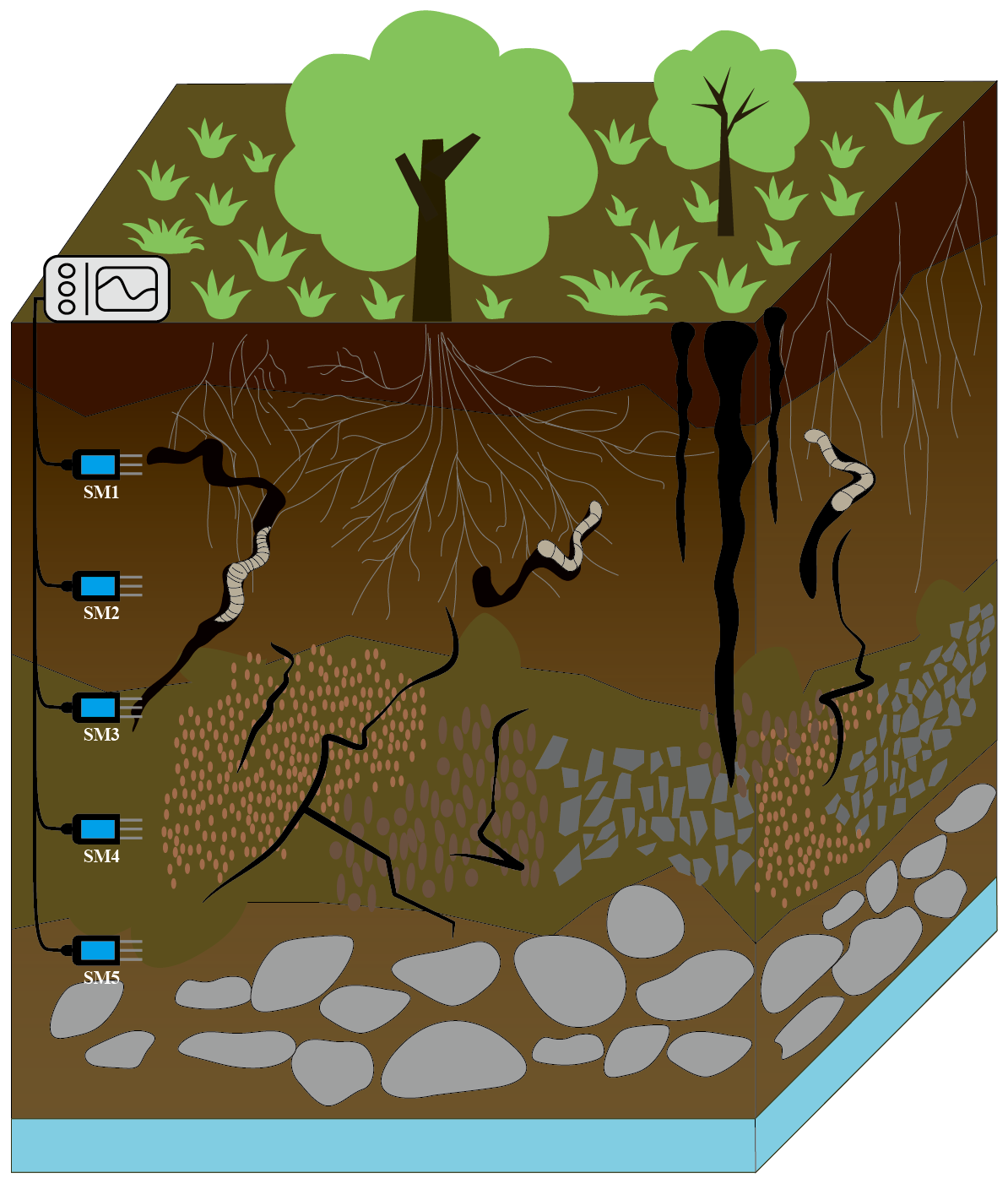
Figure 1 Examples of complex soil conditions related to soil texture and soil structure at the soil profile scale.SM3 is more related to SM1 other than SM2 or SM4, due to the existence of wormholes. The proposed non-local neural network is designed to understand that SM3 is highly correlated with SM1 (caused by fast water migration in wormholes) and less correlated with SM2 (caused by slow seepage under gravity).

In recent years, deep learning (Lecun et al., 2015) has gained considerable attention for its remarkable capabilities in fitting to complex data patterns. When predicting soil moisture, deep learning primarily relies on modeling temporal dependencies. The fundamental models handling sequential data fall into three categories: Recurrent Neural Networks (RNNs) (Elman, 1990), Convolution Neural Networks (CNNs) (LeCun, 1989), and Transformers (Vaswani et al., 2017). RNNs exploit temporal dependencies through recurrent operations, with Long Short-Term Memory (LSTM) networks demonstrating accurate soil moisture predictions (Fang et al., 2019). CNNs capture dependencies with repetitive convolutional operations and also yield satisfactory results in soil moisture dynamics modeling (Severyn and Moschitti, 2015; Shi et al., 2015). Both recurrent and convolutional operations process local neighborhoods in input data. Consequently, long-range dependencies are captured through repeated local operations, which is inefficient (Zhu et al., 2021). In contrast, Transformers process data in a more efficient way, owing to its core component – self-attention mechanisms. These mechanisms extract crucial long-range non-local information directly. For instance, Temporal Fusion Transformers with interpretable self-attention layers have shown significant improvements over existing benchmarks in multi-horizon time series forecasting (Lim et al., 2021). Furthermore, Transformers exhibit potential for effective soil moisture dynamics prediction with straightforward model structures (Wang et al., 2024). Researchers are increasingly recognizing the potential of Transformers.

However, it is worth noting that current deep learning models often lack physical laws and interpretability. To bridge the gap between data-driven approaches and physics, physical principles can be embedded into loss functions or model architectures. Some researchers have added the residuals of governing physical equations to the loss function, giving rise to Physics-informed Neural Networks (PINN) (Raissi et al., 2017, 2019). In terms of model architectures, Jiang et al. (2020) integrated the physical processes from a conceptual hydrological model into an RNN for runoff modeling. De Bézenac et al. (2018) incorporated advection-diffusion principles into the kernel design of a CNN to predict sea surface temperature. To date, most previous works have relied on traditional model structures, leaving a critical gap in reliable data-driven methods for soil moisture prediction. This underscores the necessity of transitioning toward soil science-informed machine learning models that use the power of data-driven techniques while integrating soil science knowledge during the training process to enhance reliability and generalizability (Minasny et al., 2024).

Considering that physical models calculate soil moisture content by iteratively using current soil profile states for stepwise predictions, we incorporate the spatial interactions of soil moisture within the profile into our machine learning model. We intend to update soil moisture at each depth based on the states of all depths, with predictions computed as a weighted aggregation of the previous states. When dealing with relationships between multiple variables, geometric deep learning (Bronstein et al., 2017) defines model invariances to enhance robustness and generalization. As an example, graph neural networks (GNNs) (Scarselli et al., 2008) utilize the adjacency matrix to aggregate node features and achieve local invariance. Wang et al. (2025) proposes a spatiotemporal graph convolutional network that models inter-station relationships to effectively predict soil moisture. While GNNs aggregate information through graph-structured neighborhood relationships, Non-local Neural Networks (NLNNs) directly model pairwise dependencies among all positions (Wang et al., 2018). This fully connected interaction pattern allows each position to directly interact with all other positions, thereby enabling the model to capture long-range global dependencies. The interaction weights are adaptively determined by the real-time soil moisture state in a fully data-driven manner. This fundamental difference reflects distinct inductive biases: GNNs rely on graph-structured message passing, whereas NLNNs explicitly model global interactions without neighborhood restrictions. For soil moisture dynamics, where relevant dependencies may exist between distant soil layers and vary over time, such global modeling capability is particularly beneficial. The non-local operation in NLNNs calculates responses at specific locations by aggregating features from all positions in the input feature map (Wang et al., 2018). This design allows NLNNs to flexibly model global relationships in a data-driven manner, making them suitable as a general modeling module for various tasks. Considering the complexity of interactions between multi-depth soil moisture, we introduce the NLNNs to capture spatially invariant soil moisture relationships across soil layers. Our objective is to model vertical heterogeneity and inter-layer connectivity without physical assumptions. Moreover, the weights computed through non-local operations provide qualitative interpretation for model learning mechanisms. NLNNs find wide application in image segmentation tasks and time series forecasting (Liu et al., 2019; Zhu et al., 2019). As a representative of NLNNs, the Transformer is adept at processing various types of data, including images and video-related challenges (Guo et al., 2022; Khan et al., 2022; Lim et al., 2021; Liu et al., 2021; Xie et al., 2021). Furthermore, NLNNs can serve as auxiliary blocks to enhance context modeling abilities (Wang et al., 2018; Yin et al., 2020). With the flexibility of non-local operation modifications, we can envision using NLNNs to simulate the characteristics of soil water dynamics in spatial distribution while ensuring interpretability.

In this study, we have integrated NLNNs to simulate in-profile soil moisture interactions and predict multi-depth soil moisture content without physical assumptions. Our aim is to achieve accurate and effective forecasts under diverse real-world scenarios, as depicted in Fig. 1, while also providing qualitative description of intricate soil moisture dynamics, such as vertical heterogeneity and inter-layer connectivity. Specifically, we discard all assumptions on soil, root, or boundary conditions and instead attempt to learn the soil water dynamics directly from the data. Unlike traditional one-dimensional soil water flow models that often focus on adjacent-layer fluxes, our model captures complex vertical dependencies and non-uniform moisture redistribution across various depths, enhancing predictions in complex scenarios. We introduce the Self-Attention mechanism Non-local Neural Networks (SA-NLNN) to explore the potential of NLNN structures in soil moisture forecasting. Moreover, the Knowledge-Guided Non-local Neural Network (KG-NLNN) that incorporates soil water transport guidance into the non-local operation is proposed. We examine the models' interpretability using the synthetic data, while in-situ data is applied to assess the practicality and accuracy of the models. The key innovations of our study are as follows: First, unlike previous machine learning models that rely on time-series processing to capture temporal patterns, our study is designed based on a physically motivated assumption: the soil moisture profile at the current day, together with meteorological forcing, contains sufficient information to predict the soil moisture state of the following day. Therefore, the prediction task is formulated as a single-time-step problem involving multi-depth variables. This allows mutual compensation within the soil profile, enabling effective and precise soil moisture forecasts. The adaptability of NLNNs across various temporal and spatial scales is also demonstrated. Second, the learned non-local weights of the NLNN model can be visualized to provide qualitative information on soil properties inferred from soil moisture data. Each weight represents the relative influence of soil moisture at one depth on the moisture state at another depth in the subsequent time step, thereby reflecting vertical soil water interactions. The model interpretability is investigated using synthetic soil moisture data, including virtual examples of homogeneous soil, heterogeneous soil, two-layered soil, and soil with root water uptake. Third, incorporating knowledge-inspired concepts enhances model accuracy and reliability. When evaluating practical performance, we utilize in-situ soil moisture data sourced from the International Soil Moisture Network (ISMN) and compare our models with the benchmark LSTM model (Datta and Faroughi, 2023; Semwal et al., 2021; Wang et al., 2024). To the best of our knowledge, this marks the first instance of employing NLNNs for interpretable soil moisture dynamics forecasting.

The remainder of this study is organized as follows: Sect. 2 presents the NLNNs for soil moisture forecasting, including the SA-NLNN and KG-NLNN; Sect. 3 describes the synthetically generated soil moisture data and the in-situ data; Sect. 4 provides the model results and the interpretability analysis. Finally, the conclusion is drawn in Sect. 5.

2 Methodologies

2.1 Physical Background

The dynamics of soil moisture transport are fundamentally described by the Richards equation, a governing relation derived from the mass conservation law and the Buckingham-Darcy law (Buckingham, 1907). For one-dimensional uniform flow in homogeneous soil, and assuming the absence of preferential flow, this equation takes the following form:

$$\begin{array}{}\text{(1)}& {\displaystyle \frac{\partial \mathit{\theta }}{\partial t}}={\displaystyle \frac{\partial }{\partial z}}\left[K\left({\displaystyle \frac{\partial \mathit{\psi }}{\partial z}}+\mathrm{1}\right)\right]\end{array}$$

where θ [cm³ cm⁻³] is the volumetric moisture content, t [d] denotes the time, z [cm] is the vertical coordinate (positive upward), K [cm d⁻¹] is the unsaturated hydraulic conductivity, ψ [cm] is the soil matric potential of water.

Based on this equation, the soil moisture profile at a subsequent time step evolves from the preceding profile. Infiltration and evaporation, driven by meteorological factors, directly influence surface soil moisture, which triggers a redistribution of moisture through the soil profile. Therefore, the multi-depth soil moisture at the next time step can be determined by both the current meteorological conditions and the soil moisture profile from the previous time step.

2.2 Model structures

According to Sect. 2.1, we assume that the soil moisture within the profile at the next time step depends on both the current meteorological conditions and the soil moisture from the previous time step in our soil moisture forecasts at multiple depths. The NLNN models are designed to capture the potential interactions of soil moisture at different depths within the vertical profile (Fig. 1), thereby making predictions that are closer to reality. Figure 2 illustrates the NLNN structure proposed for soil moisture dynamics prediction. The input data for the NLNN model, denoted as X^t= [$x_{\mathrm{0}}^t$, $x_{\mathrm{1}}^t$, $x_{\mathrm{2}}^t$, …, $x_{n-\mathrm{1}}^t$, $x_n^t]$, comprises a concatenation of soil moisture truth at n depths from the previous time step ${\mathrm{sm}}^t=[{\mathrm{sm}}_{\mathrm{1}}^t,{\mathrm{sm}}_{\mathrm{2}}^t,\mathrm{\dots },{\mathrm{sm}}_n^t{]}^{\mathrm{T}}$ and the upper boundary factor $x_{\mathrm{0}}^t$ obtained from meteorological conditions processing through an LSTM. Here, ${\mathrm{sm}}_n^t$ denotes the soil moisture at depth n and time t. The initial soil moisture content for the prediction is set to the truth from the preceding day. Specifically, this value is obtained from the physical model's output for the virtual scenario and from field observations for the real-world scenario.

Within our framework, we employ two types of non-local operations. The first, SA-NLNN, utilizes embedded Gaussian functions; it represents a novel application of the self-attention mechanism to capture vertical dependencies in soil moisture. The second model, KG-NLNN, is a newly proposed architecture where the non-local operation is decoupled based on the soil water transport mechanisms. In the NLNN structure, following the non-local operation and a residual connection, a fully connected neural network is employed to generate predictions for the soil moisture at each corresponding depth. This yields prediction denoted as, ${\mathrm{sm}}^{t+\mathrm{1}\prime }=[{\mathrm{sm}}_{\mathrm{1}}^{t+\mathrm{1}\prime },{\mathrm{sm}}_{\mathrm{2}}^{t+\mathrm{1}\prime },\mathrm{\dots },{\mathrm{sm}}_{n-\mathrm{1}}^{t+\mathrm{1}\prime },{\mathrm{sm}}_n^{t+\mathrm{1}\prime }{]}^T$. The ground truth is represented as ${\mathrm{sm}}^{t+\mathrm{1}}=[{\mathrm{sm}}_{\mathrm{1}}^{t+\mathrm{1}},{\mathrm{sm}}_{\mathrm{2}}^{t+\mathrm{1}},\mathrm{\dots },{\mathrm{sm}}_{n-\mathrm{1}}^{t+\mathrm{1}},{\mathrm{sm}}_n^{t+\mathrm{1}}{]}^T$. The model is trained by minimizing the error between predictions and the ground truth.

2.3 Non-local Operations

The general form of a non-local operation in NLNNs can be defined as follows (Wang et al., 2018):

$$\begin{array}{}\text{(2)}& {\mathit{y}}_i={\displaystyle \frac{\mathrm{1}}{C\left(\mathit{x}\right)}}\sum _{\forall j}f({\mathit{x}}_i,{\mathit{x}}_j)g\left({\mathit{x}}_j\right)\end{array}$$

Here i denotes the index of the output y for which the output value is being calculated, while j is the index that lists all conceivable positions in the input x. The term y_i denotes the ith component of the output y. In this context, x represents the input data and y denotes the corresponding output, both sharing the same dimensionality. In this work, x represents the concatenation of input soil moisture data and upper boundary condition data, denoted as sm^t. Accordingly, x_i and x_j denote the soil moisture at the ith and jth depths at time step t, ${\mathrm{sm}}_i^t$ and ${\mathrm{sm}}_j^t$. The output y corresponds to the predicted soil moisture at the next time step, denoted as ${\mathrm{sm}}^{t+\mathrm{1}\prime }$, where y_i represents the predicted soil moisture content at the ith depth, ${\mathrm{sm}}_i^{t+\mathrm{1}\prime }$. The computation of a generic non-local operation involves three components: the pairwise function f, the unary function g, and the normalization sum C(x). The function f calculates a scalar (representing relationship such as affinity) between i and all j, while the unary function g generates a representation of the input at position j. The aggregated response is then normalized by C(x). In this study, the form of g is restricted to a linear embedding: g(x_j)=W_gx_j, where W_g is a learnable weight matrix. The primary modification focuses on the pairwise function f. The C(x) is contingent on the design of f. Following the definition of attention heads from previous work on self-attention mechanisms (Vaswani et al., 2017), our NLNN models employ several operation heads to enhance the model's feature extraction and representation capabilities. The number of operation heads is denoted as n_head. Similar non-local operations are performed in each head, with some parameter matrices being unique. To form the output, results from each head are concatenated, and a parameterized linear transformation is applied.

The non-local operations offer flexibility by assuming various forms and can adapt to specific problem designs. This provides potential solutions for many complex situations. This flexibility stems from their ability to model global dependencies through data-dependent pairwise interactions. Among these formulations, the Transformer represents the most typical and widely used architectural instantiation, which models global dependencies through the query–key–value self-attention mechanism, multi-head attention, positional encoding, and feed-forward layers. From a more general perspective, the Non-local Neural Network can be viewed as a broader formulation of non-local dependency modeling, which computes interactions based on pairwise affinity functions without requiring the full Transformer architecture. In the following sections, we will introduce the classical embedded Gaussian operation, along with our knowledge-guided non-local operation designed for soil moisture dynamics.

2.3.1 Embedded Gaussian Operation:

Self-attention, a specific case of non-local operations within the embedded Gaussian version, is a key component of the Transformer architecture. It excels in processing data concisely and capturing intricate relationships, making it widely applied in various research areas (Devlin et al., 2019; Lim et al., 2021; Liu et al., 2021). However, it overlooks the ordering of input, necessitating the incorporation of position information into the calculations to ensure accurate processing.

Common position encoding methods include absolute position encoding (Devlin et al., 2019; Gehring et al., 2017; Vaswani et al., 2017) and relative position encoding (Shaw et al., 2018). Absolute position encoding directly incorporates absolute position information pertaining to i or j and integrates it into the input. In contrast, relative position encoding focuses on the relative relationship between position i and j. Given the complexity of soil properties and the nature of soil moisture interactions, prioritizing the relative influence of soil moisture at each depth may prove more effective than relying on absolute position information in soil moisture analysis. In this approach, we utilize the relative position encoding similar to the method proposed by Shaw et al. (2018). The function f encompasses a Gaussian function of two embeddings along with the relative position representation associated with i and j. A self-attention mechanism with relative position encodings in each head can be defined as follows:

$$\begin{array}{}\text{(3)}& {\displaystyle }f({\mathit{x}}_i,{\mathit{x}}_j)=e^{\left(\right({\mathbf{W}}_k{\mathit{x}}_j{)}^T\left({\mathbf{W}}_q{\mathit{x}}_i\right)+\mathrm{r}\mathrm{\_}{\mathrm{score}}_{ij})/\sqrt{d_k}}\text{(4)}& {\displaystyle }C\left(\mathit{x}\right)=\sum _{\forall j}f({\mathit{x}}_i,{\mathit{x}}_j)\end{array}$$

Here, W_q and W_k are the weight matrixes to be learned for embeddings. $\sqrt{d_k}$ denotes the scale factor, where d_k represents the dimension of the embeddings. r_score_ij is the relative position score computed using relative position encoding. Then the y_i can be calculated through Eq. (1). The embedded Gaussian operation for soil moisture forecasts is illustrated in Fig. 2.

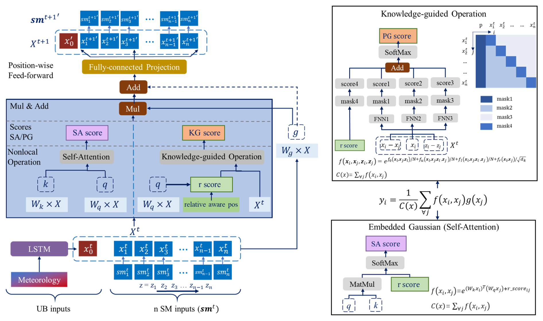
Figure 2 Left: non-local neural network structure for soil moisture forecasting. Right: embedded Gaussian operation and knowledge-guided non-local operation. RPE: relative position encoding. SA/KG score: non-local weights computed through embedded Gaussian operation and knowledge-guided operation. W_q, W_k and W_g are the weight matrixes to be learned for embeddings.

In the relative position encoding, each relationship between two arbitrary positions i and j is represented by a learnable vector. Here, r_score_ij denotes an internal relative position score used in the non-local operation, rather than a model evaluation metric. Then, the r_score_ij is calculated as follows:

$$\begin{array}{}\text{(5)}& \mathrm{r}\mathrm{\_}{\mathrm{score}}_{ij}=\left({\mathit{a}}_{i,j}{)}^{\mathrm{T}}\right({\mathbf{W}}_q{\mathit{x}}_i)\end{array}$$

where a_i,j represents the relative position encoding utilized for r_score_ij computing. a_i,jis a parameter vector that needs to be trained. In the proposed SA-NLNN model, our trainable relative position encoding matrix A consists of $(n+\mathrm{1})\times (n+\mathrm{1})$ distinct elements. The matrix A needs to be learned through training:

$$\begin{array}{}\text{(6)}& \mathbf{A}=\left(\begin{array}{lll}{\mathit{a}}_{\mathrm{0},\mathrm{0}}& \mathrm{\cdots }& {\mathit{a}}_{\mathrm{0},n}\\ \mathrm{⋮}& \mathrm{\ddots }& \mathrm{⋮}\\ {\mathit{a}}_{n,\mathrm{0}}& \mathrm{\cdots }& {\mathit{a}}_{n,n}\end{array}\right)\end{array}$$

In this model, all operation heads perform similar operations. W_q, W_k, and W_g are unique in each head. However, the relative position encoding can be shared across non-local operation heads.

2.3.2 Disentangled Knowledge-Guided operation

In this work, we propose KG-NLNN, a model specifically designed for forecasting soil moisture at multiple depths in the soil profile, as depicted in Fig. 2. The vertical movement of soil moisture exhibits a directional divergence: downward flow is driven primarily by gravity and constitutes a dissipation of potential energy, while upward movement is governed by capillary forces and other mechanisms acting against gravity. In this specific context, we employ a set of masks to decouple soil moisture interactions from different directions. The four masks in Fig. 2 correspond to four key components: meteorological forcing, upper soil water influence, same-depth soil moisture effects, and lower soil water interactions, respectively. Meteorological forcing, upper soil water influence, and lower soil water interactions are modeled by fully connected networks with soil moisture content and depth differences as inputs, whereas same-depth soil moisture effects are represented via relative position encoding. This knowledge-guided architecture separates different moisture movement processes for independent learning, thereby enhancing the model's ability to capture complex relationships among soil moisture variables across the soil profile.

When analyzing the soil moisture at ith depth, denoted as y_i, its dynamics are influenced by several factors: upper boundary conditions represented by x₀, upper soil moisture state at the previous time step, x_u (where u<i, primarily donated by gravity), lower soil moisture x_l, (where l<i, mainly affected by capillary), and the soil moisture at the same depth from the previous time step, x_i. Since these four components are motivated by diverse physical mechanisms, they are defined in distinct forms within the non-local operation.

Before proceeding to the subsections, we provide a brief introduction to fully-connected neural networks (FNNs) that are utilized in the following sections. A two-layer fully-connected neural network can be defined as follows:

$$\begin{array}{}\text{(7)}& \mathrm{FNN}\left({\mathit{x}}_{\mathrm{input}}\right)=a_{\mathrm{t}}\left(W_{\mathrm{2}}\right(a_{\mathrm{t}}(W_{\mathrm{1}}{\mathit{x}}_{\mathrm{input}}+b_{\mathrm{1}})+b_{\mathrm{2}})\end{array}$$

where a_t denotes the tanh activation function, and W_L and b_L represent the weight matrices and bias parameters to be learned in the Lth layer, respectively, where $L=\mathrm{1},\mathrm{2}$. x_input denotes the input vector of an FNN. According to the universal approximation theorem (Cybenko, 1989), a feedforward neural network with a single hidden layer is theoretically sufficient to approximate a wide range of nonlinear functions. In this study, a two-layer FNN is adopted to balance model expressiveness and computational efficiency. The hyperbolic tangent function is adopted as the activation function a.

The effect of upper boundary conditions on soil moisture at depth z_i is described by the function, $f_{\mathrm{0}}({\mathit{x}}_i,{\mathit{x}}_j,{\mathit{z}}_i)$, which corresponds to three factors: x₀, the meteorological factor; x_i, the soil moisture at depth z_i from the previous time step; and z_i, the depth of the concerned soil moisture. z_i denotes the ith depth in the depth vector $\mathit{z}=[z_{\mathrm{0}},z_{\mathrm{1}},\mathrm{\dots },z_n{]}^T$, which corresponds to the input soil moisture data sm^t. We utilize a two-layer FNN to describe this relationship:

$$\begin{array}{}\text{(8)}& f_{\mathrm{0}}({\mathit{x}}_i,{\mathit{x}}_j,{\mathit{z}}_i)={\mathrm{FNN}}_{\mathrm{0}}({\mathit{x}}_{\mathrm{0}},{\mathit{x}}_i,{\mathit{z}}_i),j=\mathrm{0}\end{array}$$

In considering the impacts of soil moisture in the upper layers and lower layers on soil moisture at depth z_i, we propose $f_u({\mathit{x}}_i,{\mathit{x}}_j,{\mathit{z}}_i,{\mathit{z}}_j)$ and $f_l({\mathit{x}}_i,{\mathit{x}}_j,{\mathit{z}}_i,{\mathit{z}}_j)$ to calculate the effects. Both functions are determined by the disparity in soil moisture content (x_i−x_j), the intrinsic soil moisture x_i, and the distance between two positions (z_i−z_j). As previously stated, two two-layer FNNs are employed in this section:

$$\begin{array}{}\text{(9)}& {\displaystyle }{f}_u({\mathit{x}}_i,{\mathit{x}}_j,{\mathit{z}}_i,{\mathit{z}}_j)={\mathrm{FNN}}_u({\mathit{x}}_i-{\mathit{x}}_j,{\mathit{x}}_i,{\mathit{z}}_i-{\mathit{z}}_j),i>j\text{(10)}& {\displaystyle }{f}_l({\mathit{x}}_i,{\mathit{x}}_j,{\mathit{z}}_i,{\mathit{z}}_j)={\mathrm{FNN}}_l({\mathit{x}}_i-{\mathit{x}}_j,{\mathit{x}}_i,{\mathit{z}}_i-{\mathit{z}}_j),i<j\end{array}$$

Additionally, we utilize relative position encodings to describe the soil water retention effect:

$$\begin{array}{}\text{(11)}& f_r({\mathit{x}}_i,{\mathit{x}}_j)=\mathrm{r}\mathrm{\_}{\mathrm{score}}_{ij},i=j\end{array}$$

where the relative position score r_score_ij is utilized for the water retention effect of soil moisture at a specific depth across two adjacent time steps. It can be calculated in Eq. (4). Consequently, our position encoding matrix ${\mathbf{A}}_{\mathrm{PG}}^K$ is a diagonal matrix comprising (n+1) distinct elements, which needs to be learned through training:

$$\begin{array}{}\text{(12)}& {\mathbf{A}}_{\mathrm{PG}}=\left(\begin{array}{lll}{\mathit{a}}_{\mathrm{0},\mathrm{0}}& \mathrm{\cdots }& \mathrm{0}\\ \mathrm{⋮}& \mathrm{\ddots }& \mathrm{⋮}\\ \mathrm{0}& \mathrm{\cdots }& {\mathit{a}}_{n,n}\end{array}\right)\end{array}$$

According to the above, the impact on soil moisture at a fixed depth is harmoniously coordinated and integrated through the four components mentioned earlier, as illustrated in Fig. 2. Therefore, the knowledge-guided non-local operation for soil moisture dynamics simulation can be defined as follows:

$$\begin{array}{}\text{(13)}& {\displaystyle }\begin{array}{rl}f& ({\mathit{x}}_i,{\mathit{x}}_j,{\mathit{z}}_i,{\mathit{z}}_j)\\ & =e^{f_{\mathrm{0}}({\mathit{x}}_i,{\mathit{x}}_j,{\mathit{z}}_i)/N+f_u({\mathit{x}}_i,{\mathit{x}}_j,{\mathit{z}}_i,{\mathit{z}}_j)/N+f_l({\mathit{x}}_i,{\mathit{x}}_j,{\mathit{z}}_i,{\mathit{z}}_j)/N+f_r({\mathit{x}}_i,{\mathit{x}}_j)/\sqrt{d_k}}\end{array}\text{(14)}& {\displaystyle }C\left(\mathit{x}\right)=\sum _{\forall j}f({\mathit{x}}_i,{\mathit{x}}_j,{\mathit{z}}_i,{\mathit{z}}_j)\end{array}$$

where N is the number of positions in x, $\sqrt{d_k}$ denotes the scale factor. Then y_i can be calculated using Eq. (1). All operation heads execute similar operations in this model. W_q utilized for r_score computing and W_g in g(x_j) are still unique in each head. The parameters of the FNNs are shared across non-local operation heads.

2.4 Boundary processing

In our soil moisture prediction task, the impact of the upper boundary conditions on soil moisture is partially simulated by an LSTM module (Hochreiter and Schmidhuber, 1997), as illustrated in Fig. 2. We have selected six meteorological variables to characterize the influence of these upper boundary conditions: precipitation (P), air temperature (AT), long-wave radiation (LR), short-wave radiation (SR), relative humidity (RH), and wind speed (WS). These variables, denoted as ${\mathrm{ub}}^t=[P^t,{\mathrm{AT}}^t,{\mathrm{LR}}^t,{\mathrm{SR}}^t,{\mathrm{RH}}^t,{\mathrm{WS}}^t{]}^{\mathrm{T}}$, are closely associated with the infiltration and evapotranspiration processes. Hydrologically, meteorological conditions from the previous time step (t−1) do not cease their influence immediately; rather, processes such as infiltration, lateral flow, and redistribution allow these conditions to continue affecting soil moisture at the subsequent time step t. Incorporating both time steps thus enables the model to capture cross-day causal relationships. A time step of 2 is used to keep the meteorological inputs concise while retaining adequate informational richness. Accordingly, the task of learning meteorological temporal dependencies is assigned to the LSTM network, which also justifies its use in processing boundary conditions. Following LSTM processing, the impact of the upper boundary conditions takes the form of ${\mathrm{sm}}_{\mathrm{0}}^t$, which is subsequently utilized in non-local operations in conjunction with the input soil moisture data $[{\mathrm{sm}}_{\mathrm{1}}^t,{\mathrm{sm}}_{\mathrm{2}}^t,\mathrm{\dots },{\mathrm{sm}}_{n-\mathrm{1}}^t,{\mathrm{sm}}_n^t{]}^{\mathrm{T}}$ within the soil profile. The operation of an LSTM can be summarized as follows:

$$\begin{array}{}\text{(15)}& {\displaystyle }{i}^t=a_{\mathrm{s}}(W_{\mathrm{i}}\cdot [h^{t-\mathrm{1}},{\mathrm{ub}}^t]+b_{\mathrm{i}})\text{(16)}& {\displaystyle }{f}^t=a_{\mathrm{s}}(W_{\mathrm{f}}\cdot [h^{t-\mathrm{1}},{\mathrm{ub}}^t]+b_{\mathrm{f}})\text{(17)}& {\displaystyle }{o}^t=a_{\mathrm{s}}(W_{\mathrm{o}}\cdot [h^{t-\mathrm{1}},{\mathrm{ub}}^t]+b_{\mathrm{o}})\text{(18)}& {\displaystyle }{\stackrel{\mathrm{̃}}{C}}^t=a_{\mathrm{t}}(W_{\mathrm{c}}\cdot [h^{t-\mathrm{1}},{\mathrm{ub}}^t]+b_{\mathrm{c}})\text{(19)}& {\displaystyle }{c}^t=f^t\cdot c^{t-\mathrm{1}}+i^t\cdot {\stackrel{\mathrm{̃}}{C}}^t\text{(20)}& {\displaystyle }{h}^t=o^t\cdot a_{\mathrm{t}}\left(c^t\right)\end{array}$$

where W_i and b_i, W_f and b_f, W_o and b_o denote the deep learning parameters for the input gate, forget gate, and the output gate, respectively; W_c and b_c are the parameters for cell state updating; in addition, i^t, f^t and o^t are the input gate, forget gate, and output gate at time t, respectively, and c^t is the memory cell state; h^t represents the hidden state; a_s is the sigmoid activation function, and a_t denotes the tanh activation function.

Through sequential processing, the last hidden state h^t in the output $[h^{t-\mathrm{1}},h^t]$ derived from input $[{\mathrm{ub}}^{t-\mathrm{1}},{\mathrm{ub}}^t]$, which encodes the upper boundary effect over two time steps, is adopted as the ${\mathrm{sm}}_{\mathrm{0}}^t$. In this study, the lower boundary conditions are disregarded due to the obstacles in observation.

2.5 Training Strategies

The objective of our model is to simultaneously predict soil moisture at multiple depths for the next time step. To achieve this, we define the loss function as the sum of squared errors between the model predictions and the corresponding ground truth of soil moisture content at different depths. The model is trained by minimizing this loss function:

$$\begin{array}{}\text{(21)}& L=\sum _{t=\mathrm{0}}^B\sum _{i=\mathrm{1}}^n({\mathrm{sm}}_i^{t+\mathrm{1}\prime }-{\mathrm{sm}}_i^{t+\mathrm{1}}{)}^{\mathrm{2}}\end{array}$$

where n denotes the number of concerned soil moisture depths, and B is the training batch size, which is set to 100 in this study.

In this work, the collected data is divided into training, validation, and test sets in a time-ordered ratio of 6 : 2 : 2. For training, we employ the Adam optimizer (Kingma and Ba, 2015) with a learning rate of 0.001. The models are trained for a minimum of 2500 epochs, with 20 batches in each epoch. The validation set is utilized to select the best model and mitigate overfitting. Subsequently, the test set is then employed to evaluate the performance of the models. Each result is computed based on 10 replicates with different initializations. Regarding the model hyperparameter settings, in the non-local neural network, we set $d_k=d_q=\mathrm{10},d_g=\mathrm{16},$ and n_head=10, where d_k, d_q and d_g represents the dimensions of the key, query and value (function g) components within the non-local block, respectively. n_head denotes the number of non-local heads. The LSTM consists of two stacked blocks, each configured with a hidden layer of 20 neurons. In the FNN adopted for KG-NLNN, we utilize 10 neurons in each hidden layer.

3 Data Descriptions

In our study, synthetic soil moisture data is generated to investigate the interpretability of these NLNN models. Additionally, we utilize the selected in-situ soil moisture data to assess the accuracy and practicability of our models.

3.1 Synthetic Data Description

The synthetic data are generated using the ROSS method (Ross, 2003, 2006). The Ross method is a rapid, non-iterative numerical scheme for soil moisture forward modeling. In our simulation, we create soil moisture content data for a 100 cm soil column with 1 cm intervals. For boundary conditions, the daily reference evapotranspiration (ET0) is calculated with the FAO Penman-Monteith method (Allen et al., 1998) in Wuhan coordinates to generate the synthetic data. As standardized in the FAO guidelines (Allen et al., 1998), actual evapotranspiration is the product of K_C and ET0, where K_C serves as a refined empirical parameter. When generating synthetic data, we applied this empirical coefficient method to derive a preliminary evapotranspiration estimate, adopting a coefficient value of 1.0 in this instance. The daily time series data of precipitation and calculated evapotranspiration are shown in Fig. 3. The lower boundary condition is set as free drainage, and the initial moisture content of the soil column is set to a uniform value of 0.10. We generate three years of time series soil moisture data for this research.

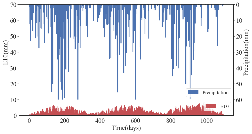
Figure 3 Daily time series precipitation and reference evapotranspiration data calculated at Wuhan coordinate for generating synthetic data.

In this section, we design four virtual cases of different configurations to investigate model interpretability, including homogeneous soil, heterogeneous soil, two-layered soil, and soil with root water uptake scenarios, as represented in Fig. 4. When generating synthetic data in the case with root water uptake, the root depth is set to 50 cm, and root density is vertically distributed evenly. Detailed soil property settings are given in Appendix A. Besides, we assess the adaptability across different time scales and observation locations using the available data.

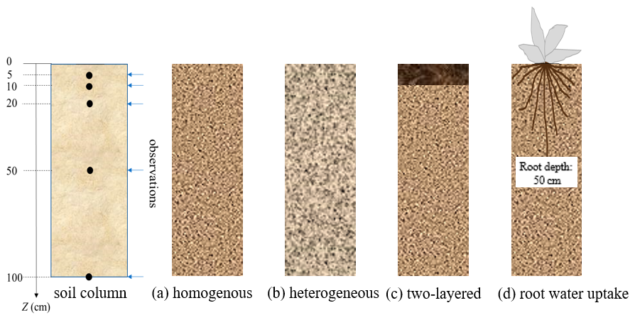
Figure 4 The virtual cases design, with homogeneous soil (a), heterogeneous soil (b), two-layered soil (c), and homogeneous soil with root water uptake (d).

3.2 In-situ Data Description

To comprehensively evaluate the proposed NLNN models, we carefully select soil moisture content observations from twenty sites within the International Soil Moisture Network (ISMN) (https://ismn.earth/en/, last access: 12 May 2026.). These sites are chosen based on geographical locations, soil textures, and land cover types. Detailed information for the selected sites is presented in Table 1, and their spatial locations are illustrated in Fig. 5. These carefully selected sites encompass 16 soil types and 6 land cover species, providing a diverse range to assess the model's performance and its ability to adapt to complex soil situations. At each site, in-situ observations are required to include soil moisture observations at 5 standard depths (0.05, 0.10, 0.20, 0.50, 1.00 m).

Table 1 Summary of main characteristics of twenty selected sites.

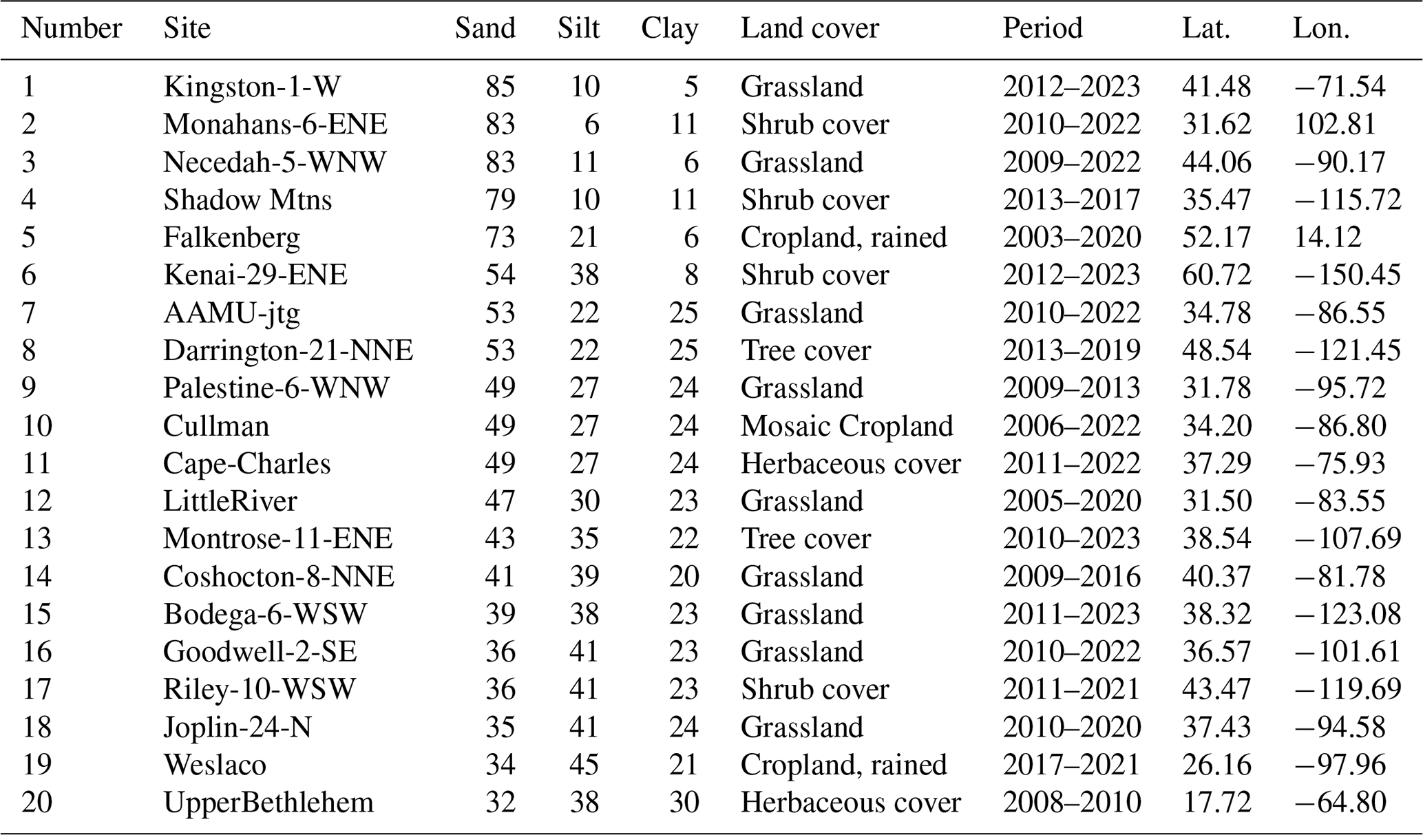
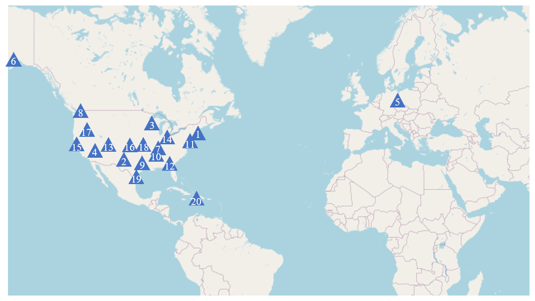
Figure 5 The spatial locations of twenty selected sites. The numbers on the sites correspond to the serial numbers in Table 1.

The meteorological inputs for our models include precipitation, atmospheric temperature, long-wave radiation, short-wave radiation, wind speed, and relative humidity, as mentioned above. These meteorological data are sourced from the NASA Prediction of Worldwide Energy Resources project (https://power.larc.nasa.gov/, last access: 12 May 2026). Based on the latitude and longitude coordinates of each station, we downloaded the corresponding point-scale, daily-resolution meteorological datasets. Detailed information about this can be found at (https://power.larc.nasa.gov/docs/methodology/meteorology/, last access: 12 May 2026). Unfortunately, due to challenges in obtaining groundwater level observations, changes in the lower boundary conditions are not considered in this study.

4 Results and discussions

In this study, we systematically examine and analyze our models from three perspectives. Initially, we assess the essential capabilities of models, including accuracy and uncertainty, using both synthetic data and in-situ observations. Subsequently, we apply simulated soil moisture data under diverse virtual scenarios to evaluate our model's interpretability and its ability to provide qualitative interpretations depicting soil moisture interaction mechanisms across diverse depths within the profile. Finally, we investigate the impacts of varying temporal scales, noise levels, and observation locations on our non-local neural networks.

To explore the forecasting ability of our models over time series, we examine predictions for 1, 3, and 7 d ahead at selected sites, as well as 1, 3, 7, and 15 d ahead for simulated data. We generate predictions iteratively. The evaluation standards in this work comprise the mean absolute error (MAE) and the root mean square error (RMSE). Both MAE and RMSE quantify the deviation between the predictions and the ground truth. However, RMSE exhibits greater sensitivity to outliers due to its squaring of deviations, which amplifies the impact of extreme values, while MAE offers a smoother average error value. These metrics are calculated as follows:

$$\begin{array}{}\text{(22)}& {\displaystyle }\mathrm{MAE}={\displaystyle \frac{{\sum }_{i=\mathrm{1}}^{N_{\mathrm{s}}}|T_i-{\widehat{T}}_i|}{N_{\mathrm{s}}}}\text{(23)}& {\displaystyle }\mathrm{RMSE}=\sqrt{{\displaystyle \frac{{\sum }_{i=\mathrm{1}}^{N_{\mathrm{s}}}(T_i-{\widehat{T}}_i{)}^{\mathrm{2}}}{N_{\mathrm{s}}}}}\end{array}$$

where ${\widehat{T}}_i$ and T_i represent the predictions and the ground truth, respectively; ${\stackrel{\mathrm{‾}}{T}}_i$ is the average of the ground truth; N_s is the test sample size. Here, T denotes the soil moisture content [%] which needs to be calculated. All the compared models are trained and evaluated using the same datasets, input variables, and evaluation metrics to further ensure consistency and fairness in the comparison.

When conducting uncertainty analysis, evaluating confidence bounds becomes challenging because most deep learning neural networks are essentially deterministic models. To address this, many researchers utilize the bootstrap aggregating (bagging) method (Breiman, 1996) to analyze model predictive uncertainty (Kornelsen and Coulibaly, 2014). The bagging method involves training multiple neural network models using subsets of the training set, all with identical architecture. To create the training subset for each model, a statistical bootstrap approach is employed. For each subset, we randomly select individual input vectors from the entire training set with replacement, ensuring that each subset contains the same number of elements as the entire training set. After training, we obtain an ensemble of trained models, each trained with a unique training subset. The final output and uncertainty estimates are then derived from the mean and standard deviation of this ensemble.

To explore the impact of noise on our models using the synthetic data, we apply the zero-mean Gaussian noise with a variance of 1:

$$\begin{array}{}\text{(24)}& \dot{\mathit{\theta }}=\mathit{\theta }+\mathit{\eta }\cdot N(\mathrm{0},\mathrm{1})\end{array}$$

where $\dot{\mathit{\theta }}$ is the volumetric soil moisture content with noise [%], and θ is the synthetic volumetric soil moisture content. Three noise levels are tested (η= 0.5, 1.0, 2.0) in this work.

In our investigation of model interpretability, the visualized non-local weight maps generated from the output play a crucial role as evaluation standards. According to Eq. (2), the normalized weights $\frac{\mathrm{1}}{C\left(\mathit{x}\right)}f({\mathit{x}}_i,{\mathit{x}}_j)$ quantify the relative influence of soil moisture at depth j on the prediction at depth i. These normalized interaction weights reflect how strongly soil moisture information from different depths on the previous day contributes to the predicted soil moisture at a given depth on the following day. These weight maps may provide qualitative interpretations depicting intricate mechanisms of soil water dynamics. The color brightness on the weight distribution map signifies the level of interaction strength among upper boundary conditions and soil moisture across different depths. Therefore, analyzing the weight matrix map is essential for gaining insights into the learning mechanisms of our NLNN models.

4.1 Interpretability analysis

Before the models can be applied to real-world scenarios, their stability and interpretability must first be analyzed. In this section, we explore the interpretability of the NLNN models by designing several scenarios that generate synthetic data. These simulated cases primarily involve variations in soil properties, including homogeneous soil, heterogeneous soil, two-layered soil, and soil with root water uptake scenarios. We benchmark the soil moisture prediction tasks against the LSTM model, widely used in time series forecasting (Datta and Faroughi, 2023; Ding et al., 2019; Siami-Namini et al., 2019). Specifically, the LSTM model takes two forms tailored for different data processing approaches: LSTM_T, which utilizes input data from the previous four time steps to predict soil moisture content at the next time step. It follows a configuration similar to that in previous work (Wang et al., 2024). These predictions rely on modeling temporal dependencies. In contrast, LSTM_I replaces the non-local operations in the architecture shown in Fig. 2 with LSTM modules, thereby modeling interactions among soil water layers. It represents the predictive capabilities achievable by a single-time-step LSTM. With the synthetic data, we investigate the model performance and interpretability through the weight matrix maps and delve into their learning mechanisms across diverse scenarios.

Figure 6 displays the RMSE results for 1, 3, 7, and 15 d forecasts of four models, and the MAE values of four simulated scenarios are summarized in Appendix C. As shown in Fig. 6, the LSTM_T model achieves very high accuracy in 1 d predictions, but its performance deteriorates rapidly over longer periods. As for the other models, NLNNs and LSTM_I exhibit comparable performance. The knowledge-guided model KG-NLNN exhibits lower variance and maintains greater stability in RMSE, especially in the 15 d prediction task. The integration of knowledge guidance proves crucial in ensuring model stability.

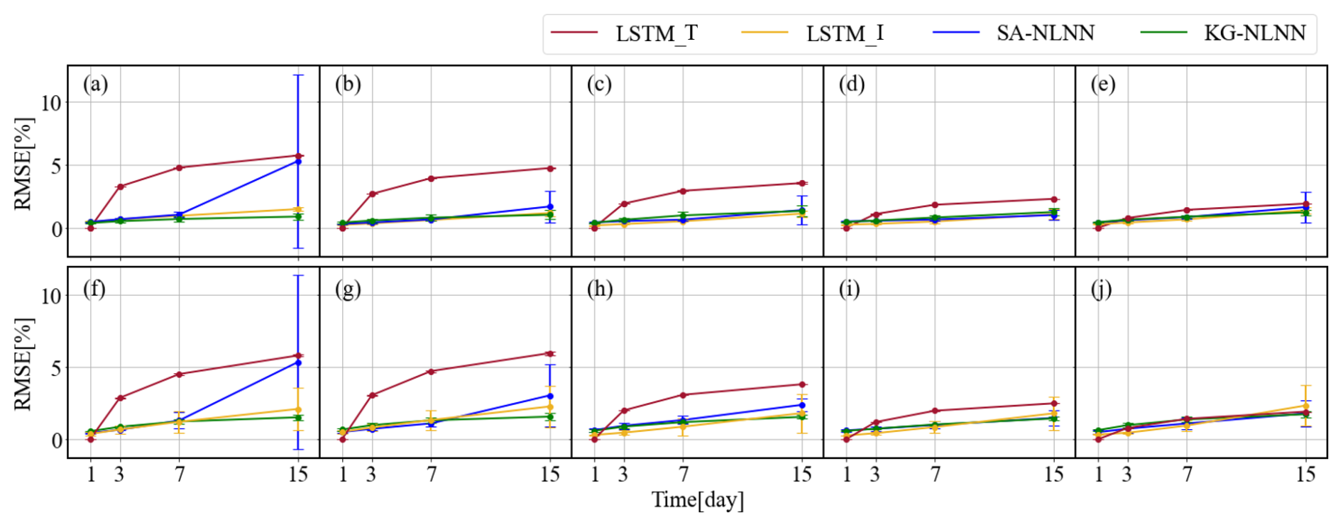
Figure 6 The RMSE results for 1, 3, 7, and 15 d for heterogeneous soil (a–e), and two-layered soil (f–j). The error bar indicates the standard deviations of the RMSE, which are computed via ten training replicates.

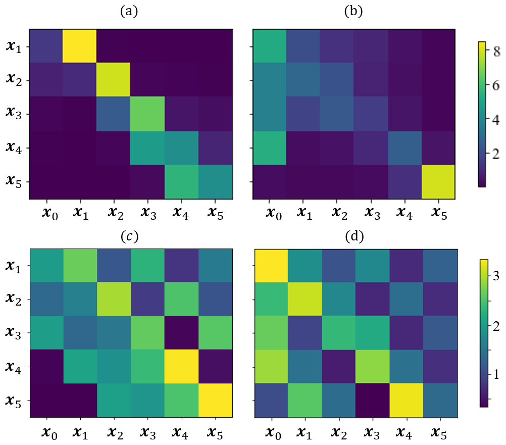
Figure 7 The non-local weight maps in homogeneous simulated soil scenarios through KG-NLNN (a) K_s= 0.25 (b) K_s= 10.49, and SA-NLNN (c) K_s= 0.25, (d) K_s= 10.49.

Figure 7 depicts the weight matrix maps generated by KG-NLNN and SA-NLNN models for homogeneous soil scenarios varying saturated hydraulic conductivity (K_s) values. These maps represent the term $\frac{f({\mathit{x}}_i,{\mathit{x}}_j)}{C\left(\mathit{x}\right)}$ calculated through non-local operations. Each element at position (i,j) represents the impact of soil moisture at depth z_j at the previous time on the soil moisture content at depth z_i. Notably, when j=0, it signifies the influence of upper boundary conditions on soil moisture across various depths. The brightness level corresponds to the strength of this influence, with higher brightness indicating a stronger impact. Homogeneous soil scenarios with different K_s values are used to examine variations in the non-local weight matrices. The weight maps produced by the KG-NLNN model exhibit clear and stable spatial patterns across different K_s, whereas the SA-NLNN results appear relatively chaotic, indicating that a knowledge-guided structural design can serve as a valuable enhancement.

Differences in hydraulic conductivity govern soil water flow velocity, leading to variations in the time required for water to reach different depths. These differences shape the structure of the weight maps and give rise to the distinct patterns observed in Fig. 7a and b. For instance, loam (K_s= 0.25) exhibits slow infiltration, so its moisture content is easily influenced by adjacent layers in Fig. 7a. In contrast, sand (K_s= 10.49) allows rapid infiltration, resulting in deeper soil moisture being affected directly by meteorological factors. Although the proposed model does not involve any parameterization nor perform a quantitative description of soil hydraulic parameters, it nevertheless provides insights into these hydraulic properties to some extent.

Additionally, two-layer soil scenarios are employed in which the soil properties of the upper and lower layers are exchanged to further investigate changes in the non-local weight matrices. Figure 8 depicts the weight matrix maps generated by KG-NLNN and SA-NLNN models for two-layered soil scenarios. The saturated hydraulic conductivity of the two soil types varies significantly, with distinct characteristics influencing water transport and drainage, as recorded in Appendix A. Figure 8 presents the weight matrix maps generated through KG-NLNN and SA-NLNN. Some soil structural information, such as stratification, can be reflected from the soil moisture interactions in Fig. 8a, b. In the scenario where sand is beneath loam, water gradually released from the loam layer can quickly reach various depths of the sand below. Consequently, soil moisture in the lower layers is primarily influenced by the upper loam. As shown in Fig. 8a, the moisture in the lower layer (0.10, 0.20, 0.5, 1.0 m) is notably influenced by the moisture at 0.05 m. Conversely, with sand above loam, the upper sand rapidly drains water, and the water from the upper sand is absorbed and held by the lower loam. Therefore, soil moisture in the lower layers is mainly affected by the adjacent upper layer, as shown in Fig. 8b. This layered pattern in the weight map serves as a qualitative indicator of soil texture. Although the weights do not have a direct quantitative relationship with the soil hydraulic parameters, they can reflect the difference in hydraulic conductivity between the layers and reveal which layer is more permeable.

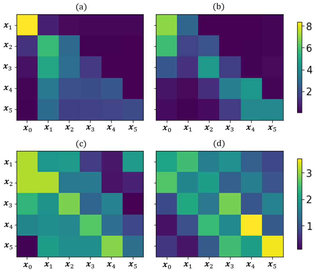
Figure 8 The non-local weight maps in two-layered simulated stratified soil scenarios through KG-NLNN (a) loam above sand (b) sand above loam, and SA-NLNN, (c) loam above sand, (d) sand above loam.

As a result, both NLNN models achieve satisfactory soil moisture forecasts in the simulated scenarios. Furthermore, the models have advanced the interpretability of machine learning through non-local weight matrix maps. Notably, KG-NLNN offers more reliable qualitative descriptions of soil properties via weights visualizations, highlighting the importance of knowledge guidance.

4.2 Performance evaluation

In this section, we evaluate the performance of the SA-NLNN and KG-NLNN models using in-situ observations from twenty ISMN sites. The performance of LSTM_T, LSTM_T, SA-NLNN, and KG-NLNN is evaluated at five different depths (0.05, 0.1, 0.2, 0.5, 1.0 m). Notably, our NLNN models predict soil moisture for all five depths simultaneously, whereas LSTM_T models each depth separately. When comparing our models with physical models, the inherent methodological differences between machine learning and physical models make fair and direct comparisons with standard knowledge-based modeling particularly challenging. We therefore limit our comparison to a preliminary assessment in Appendix B.

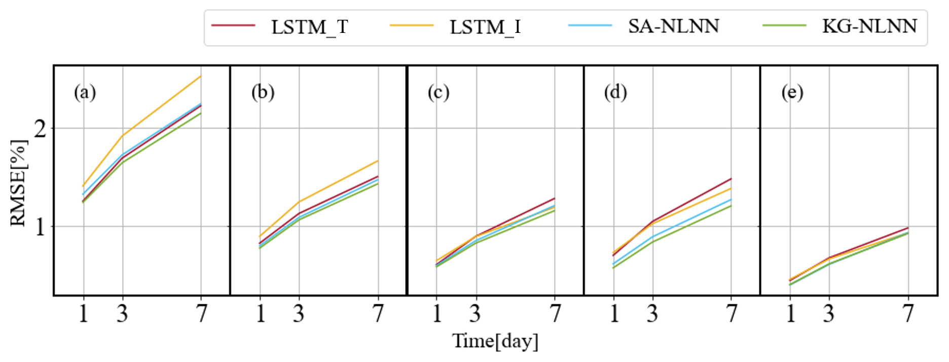
Figure 9 Comparison of mean RMSE for LSTM_T, LSTM_I, SA-NLNN, and KG-NLNN. The values are averaged across twenty research sites and presented separately for each of the five soil depths: 0.05 m (a), 0.10 m (b), 0.20 m (c), 0.50 m (d), 1.00 m (e).

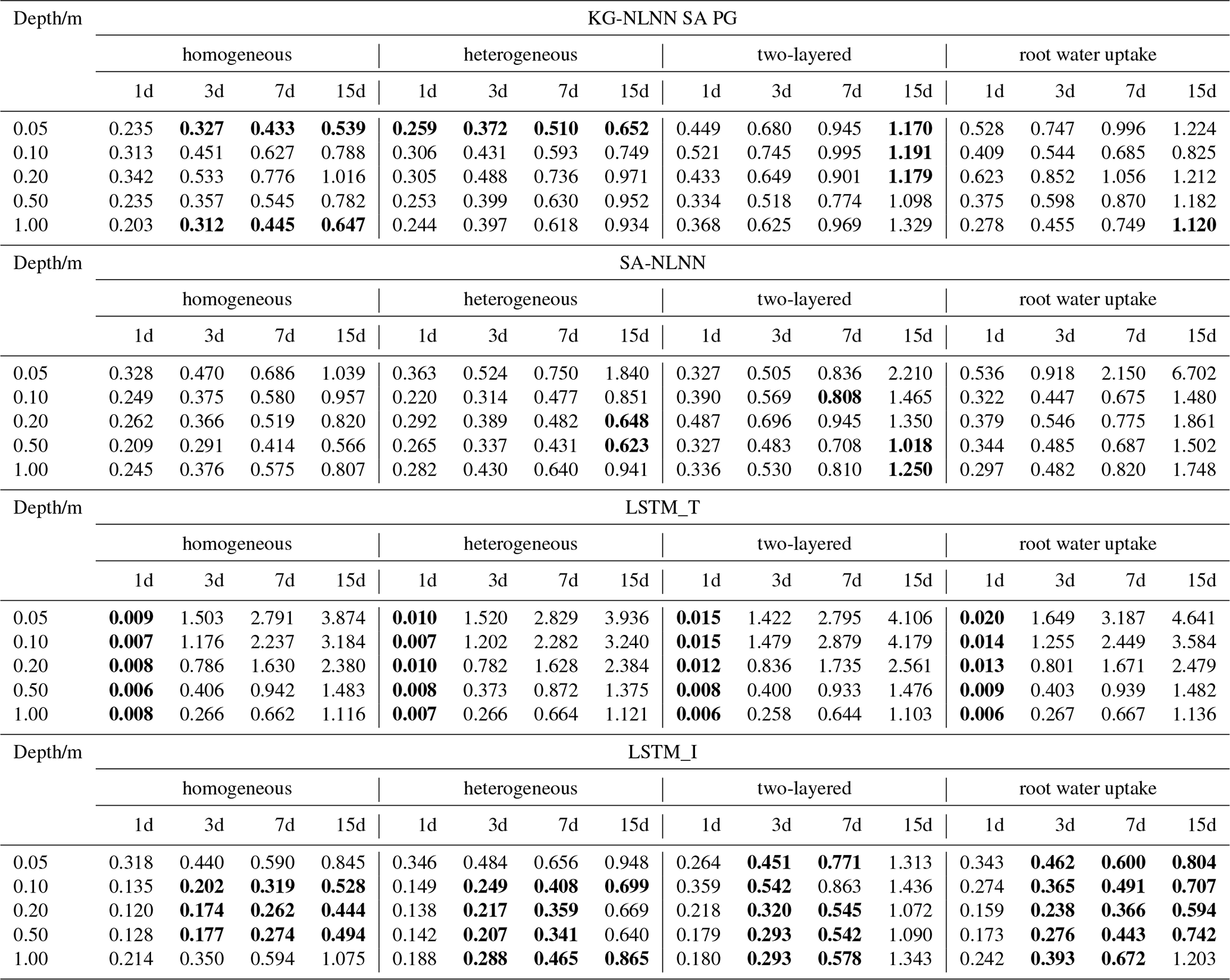
Table 2 The MAE [%] values for 1, 3, and 7 d forecasts across the four models across twenty research sites at 5 distinct depths, based on ten repeated trainings. The bold values indicate the best performance for each metric across the models.

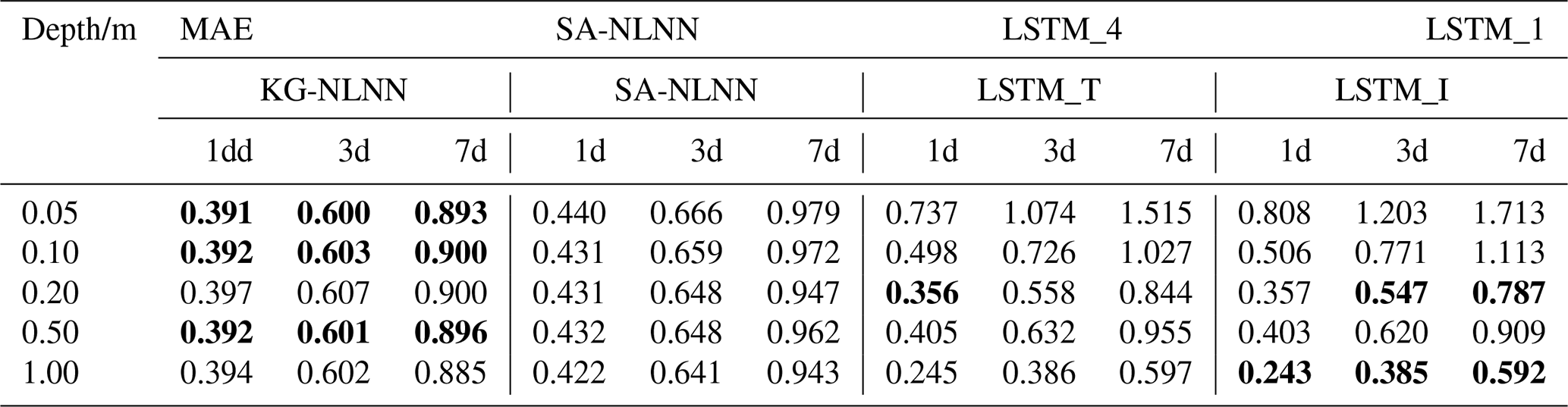
Table 2 displays the MAE values across twenty selected sites, considering forecasts for 1, 3, and 7 d from the four models at five distinct depths. These results are derived from ten repeated trainings, and the corresponding RMSE results are presented in Fig. 9. From MAE results, we observe that both LSTM_1 and LSTM_4 perform well in deep soil moisture predictions. Meanwhile, our proposed NLNN models consistently demonstrate superior accuracy at depths from 0.05 to 0.5 m. Regarding RMSE, the KG-NLNN model stands out as the best model in most situations. Figure 10 depicts the correlation between the 7 d soil moisture predictions and observations of the test set for LSTM-4, LSTM-1, SA-NLNN, and KG-NLNN. The density of scatter plots serves as an indicator of model reliability (Datta and Faroughi, 2023). The KG-NLNN model exhibits superior performance in soil moisture prediction compared to the other models, suggesting the stability of our model over longer prediction periods. The comparison between KG-NLNN and SA-NLNN underscores the value of incorporating soil water transport mechanisms into of decoupled non-local operations. Nevertheless, a limitation of the proposed NLNN models lies in their forecasts for moisture content at 1.0m. This limitation could be attributed to the absence of consideration for lower boundary conditions in our study.

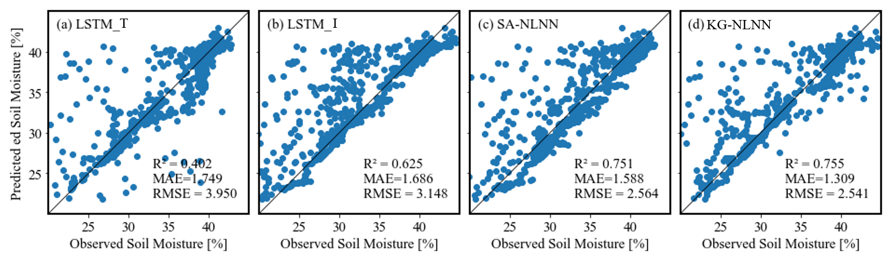
Figure 10 Scatter plots of the soil moisture observations and 7 d predictions generated from (a) LSTM_T, (b) LSTM_I, (c) SA-NLNN, and (d) KG-NLNN at UpperBethlehem.

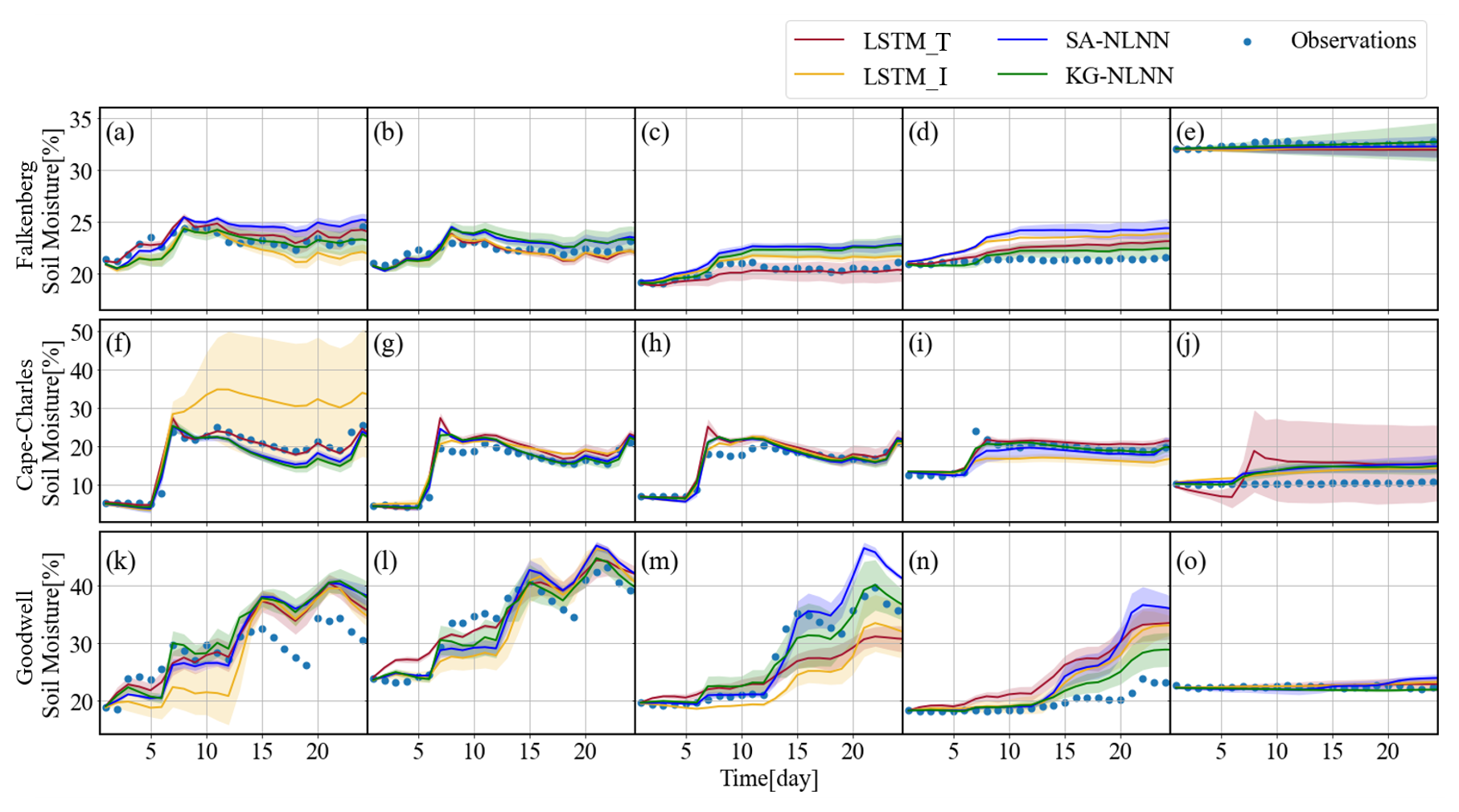
Figure 11 The autoregressive 24 d predicted soil moisture time series of 5 depths with LSTM_I, LSTM_T, KG-NLNN and SA-NLNN at Falkenberg (a–e), Cape-Charles (f–j), and Goodwell (k–o). The shaded region represents the confidence interval of the models, spanning 1 standard deviation.

Regarding how NLNN model predictions change over time, Fig. 11 displays the autoregressive 24 d predicted time series soil moisture data for the NLNN models across three sites: Falkenberg, Cape-Charles, and Goodwell. The shaded region represents the confidence interval of the models, spanning 1 standard deviation. The LSTM-based models exhibit relatively greater uncertainty in predictions. However, it is evident that both models perform satisfactorily and stably, with the proposed KG-NLNN model being closer to the observations. Considering the temporal accumulation of autoregressive errors in extended soil moisture forecasting, we provide additional long-term prediction results in Appendix B for comprehensive evaluation.

According to Sect. 4.1, the non-local weight maps can be qualitatively related to the soil properties, demonstrating the interpretability of the model. In real-world cases, even with limited soil information from the site in Table 1, we can combine the weight maps with the measured soil texture data for our analysis. Figure 12 illustrates the non-local weight matrix maps for the Falkenberg, Cape-Charles, and UpperBethlehem sites, generated by the KG-NLNN model. These maps remain stable during repeated training, with discernible variations among the three sites. They offer qualitative interpretations related to soil properties. In Fig. 12a, it is seen that at Falkenberg site, soil moisture at different depths is primarily influenced by upper boundary conditions and upper layer soil moisture. Figure 12b shows that at Cape-Charles site, soil moisture is mainly affected by upper boundary conditions and soil moisture at the same depth from the previous time step. Figure 12c depicts the strong soil water retention effect at UpperBethlehem site, soil moisture is mainly related to its own state at the previous time step. By combining Table 1, we can see that the non-local weight maps are consistent with the soil texture information. From Falkenberg to UpperBethlehem site, as the soil texture changes from sandy to clay, the learnt water retention capacity in Fig. 12 increases from low to high. Consequently, the non-local weight maps are able to capture different physical mechanisms of different sites from the measurement data.

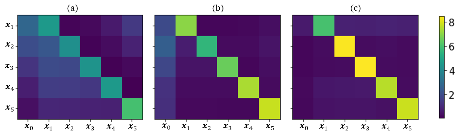
Figure 12 The non-local weight maps through the KG-NLNN at three typical sites, (a) Falkenberg, (b) Cape-Charles, and (c) UpperBethlehem.

In summary, our NLNN models achieve precise and efficient soil moisture predictions across diverse scenarios, as validated by comparisons with LSTMs using in-situ observations. Their multi-depth modeling strategy enhances overall accuracy through complementary interactions. The proposed KG-NLNN model delivers accurate predictions with low uncertainty, while also providing qualitative descriptions of the intricate soil properties. This performance underscores the necessity of incorporating soil water transport knowledge guidance in non-local operation design.

4.3 Effects of the noise levels, time scales, and observation positions

In addition to model accuracy and interpretability, our non-local neural network exhibits adaptability in prediction tasks across different time scales. In this section, we have conducted tests involving different noise levels, time intervals, and observation positions. To further investigate the impact of noise on our NLNN models, we have employed five different noise levels (0.5, 1.0, 2.0, 5.0, 10.0) and compared the NLNN model performance with LSTM models. The RMSE results for soil moisture prediction at 0.05, 0.10, 0.20, 0.50, and 1.00 m are presented in Fig. 13. The LSTM_T model demonstrates poor noise resistance and long-term forecasting capability. The other three models perform similarly under low-noise conditions, with LSTM_I even exhibiting some advantage. However, as the noise level increases, NLNN models demonstrate better robustness. Notably, the knowledge-guided NLNN is particularly stable, consistent with its performance on in-situ soil moisture data.

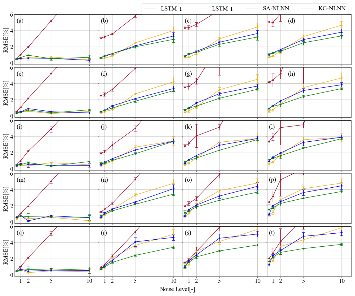
Figure 13 The RMSE results for 1, 3, 7, and 15 d at 0.05 m (a–d), 0.10 m (e–h), 0.20 m (i–l), 0.50 m (m–p) and 1.0 m (q–t) in the homogenous soil under increasing noise levels. The error bar indicates the standard deviations of the RMSE, which are computed via ten training replicates. Note: portions of the red curves are truncated where the error significantly exceeds this range, reflecting its relatively lower predictive accuracy.

When investigating the KG-NLNN model's performance at the 0.2, 0.5, and 1 d time intervals within homogenous soil, a subtle difference emerges in the weight map generated by the KG-NLNN model, as illustrated in Fig. 14. Despite a decrease in accuracy with longer time intervals, the model consistently achieves satisfactory results. The results reflect the adaptability of the model to diverse time scales.

When the number of observation locations increases to 10 (at depths of 0.05, 0.1, 0.2, 0.3, 0.4, 0.5, 0.6, 0.7, 0.8, 0.9 m), the MAE values for soil moisture 1, 3, 7, and 15 d forecasts of the NLNN models across five depths are summarized in Table 3. The uniform augmentation of measurements significantly enhances the prediction accuracy of SA-NLNN, while having minimal impact on the performance of KG-NLNN. This suggests that the knowledge guidance allows for lower requirements on soil moisture measurements. In scenarios with uniformly augmented observations, SA-NLNN may prove more efficient.

Table 3 The MAE [%] values for 1, 3, 7, and 15 d forecasts of the proposed KG-NLNN model and SA-NLNN model at 5 depths with 10 depth measurements under the homogenous soil scenario. The bold values indicate the best performance for each metric across the models.

In conclusion, both the NLNN models achieve accurate and reliable soil moisture predictions under diverse scenarios. They can adapt to tasks across different time scales. The SA-NLNN performs better under uniformly distributed observations, while the KG-NLNN demonstrates stronger noise resistance.

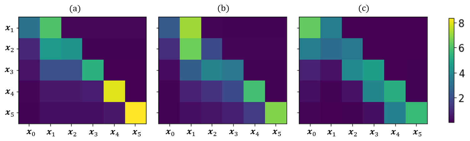
Figure 14 The non-local weight maps of the KG-NLNN model at different time scales at 0.2 d (a), 0.5 d (b), and 1.0 d (c) in the homogenous soil.

5 Conclusions

In this study, we employ the deep learning model NLNNs to achieve precise and efficient soil moisture predictions under diverse scenarios without relying physical assumptions., while providing qualitative interpretation for complex soil moisture dynamics, such as vertical heterogeneity and inter-layer connectivity. In light of the accuracy and parameter estimation challenges in physical models, and the credibility concerns in machine learning models, we have introduced a framework that integrates both accuracy and mechanistic insight. Our method leverages in-profile soil moisture interactions across various depths. Consequently, the soil moisture prediction task is reformulated as a single-time-step prediction task that involves multi-depth soil moisture variables. In this way, we apply the self-attention-based model SA-NLNN to explore the potential of the NLNN structure. Expanding on this framework, we disentangle the non-local operation into four components to create the KG-NLNN model according to the soil water transport knowledge. By comparing our NLNNs with the LSTM model using synthetic data and in-situ observations, we demonstrate that both our NLNN models achieve precise and effective forecasts, providing an alternative possibility for soil moisture simulations. The knowledge-guided model KG-NLNN exhibits the best performance and remains stable with low uncertainty. The physical knowledge guidance in non-local operations significantly enhances the model's accuracy and reliability.

Additionally, our proposed models offer qualitative interpretations related to the soil properties. Through the investigation of various virtual scenarios – including homogeneous soil, heterogeneous soil, two-layered soil, and soil with root water uptake – we observe that both the KG-NLNN and SA-NLNN models perform well in different soil conditions. The qualitative interpretations derived from soil moisture data generated by KG-NLNN facilitate descriptions of soil textures. When testing with in-situ data, we find that the KG-NLNN model also provides interpretations consistent with real soil vertical heterogeneity without physical assumptions. This highlights the importance of integrating knowledge-guided assistance into model design. Moreover, we have assessed the model's performance under different noise conditions, observation positions, and time scales. Both NLNN models exhibit robustness to noise, and the knowledge guidance enhances noise resistance. Besides, NLNN model demonstrates adaptability to diverse time scales. When observations are evenly distributed, the SA-NLNN shows significant improvements compared to KG-NLNN, while maintaining high computational efficiency.

Nevertheless, the model faces challenges that necessitate future improvements. Its training and application are site-specific, limiting its transferability. Further research is required to enhance its applicability across different sites. Specifically, difficulties arise in estimating soil moisture content at deep layers, possibly due to the lack of consideration for the groundwater boundary. Incorporating lower boundary conditions into the model could address this limitation. Additionally, multi-objective network training may benefit from more effective strategies and more precise loss function designs. Introducing constraints at multiple time steps holds promise for achieving more stable results. Finally, further refinement of the non-local operation may enhance the model's performance. What's more, the proposed network framework is architecturally flexible and modular, making it customizable for diverse research requirements. Beyond soil moisture, the NLNN-based strategy could be readily extended to other systems, such as solute transport in groundwater. We encourage the exploration of such specialized structures to address various coupled physical or hydrological problems across different scales.

Appendix A

The parameters used to generate the synthetic data are recorded in Tables A1 and A2.

Table A1 The van Genuchten soil hydraulic parameters (van Genuchten, 1980) used for synthetic data generation.

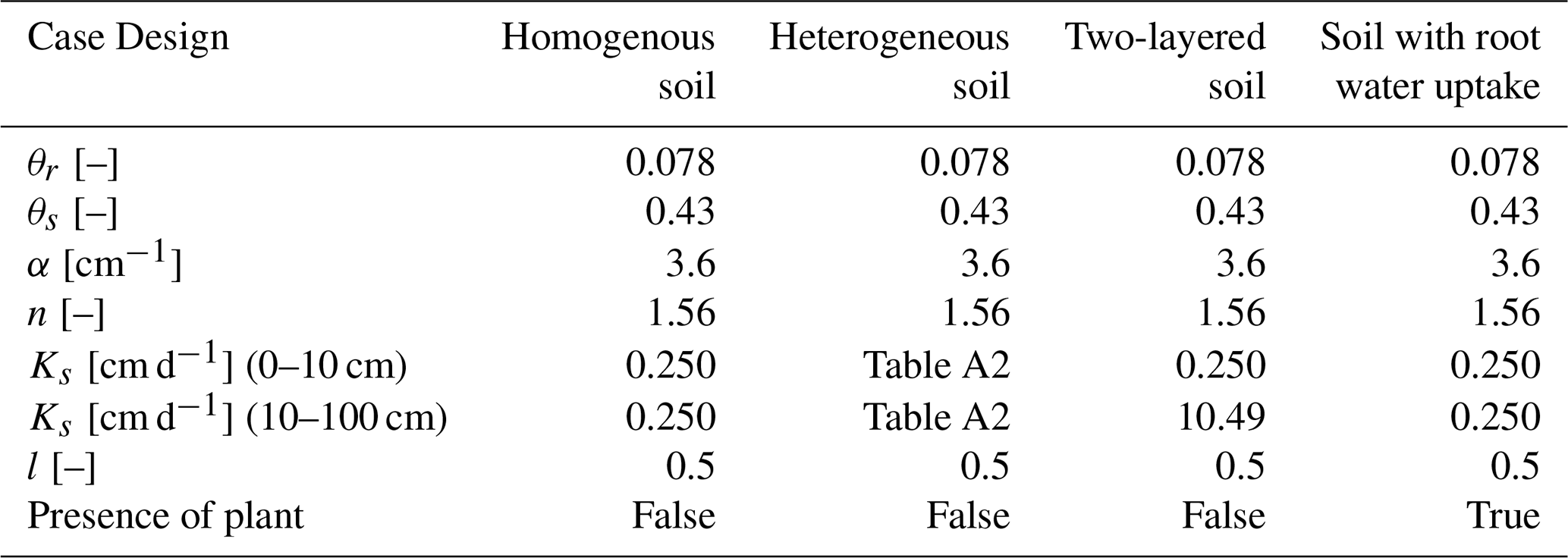
Table A2 The soil hydraulic conductivity of the heterogeneous scenario.

Appendix B

This section presents a preliminary comparison between the NLNN model and the physics-based soil moisture model derived from Richards' equation.

The Ross method (Ross, 2003, 2006) is a rapid, non-iterative numerical scheme for soil moisture forward modeling based on Richards' Equation. For boundary conditions, the daily reference evapotranspiration (ET0) is calculated with the FAO Penman-Monteith method (Allen et al., 1998). As standardized in the FAO guidelines (Allen et al., 1998), actual evapotranspiration is the product of K_C and ET0, where K_C serves as a refined empirical parameter. When generating synthetic data, we applied this empirical coefficient method to derive a preliminary evapotranspiration estimate, adopting a coefficient value of 1.0 in this instance. We first utilize 10 d of site historical data to invert the site-specific soil hydraulic parameters (α, n, K_s) through data assimilation with the ensemble Kalman filter (EnKF) method​​​​​​​​ ​​​​​​​​ (Evensen, 2003) within the Ross framework. These parameters are then applied in the Ross method to obtain a fast solution of one-dimensional Richards' equation, enabling the forecasting of soil moisture dynamics.

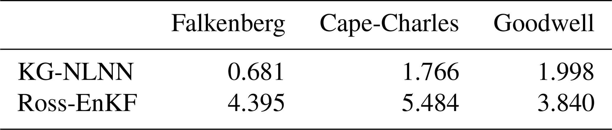
In the real-world experiments, we selected three sites: Falkenberg, Cape-Charles, and Goodwell, with distinctly different soil textures and land covers, as recorded in Table 1 in the manuscript. Figure B1 illustrates the autoregressive 24 d predicted time series soil moisture data for the KG-NLNN model and Ross-EnKF across these three sites. The MAE results are recorded in Table B1. It is seen that soil moisture forecasts obtained by KG-NLNN are closer to real observations, compared to the traditional Ross-EnKF method.

Table B1 The MAE [%] values for 24 d forecasts of the proposed KG-NLNN model and Ross-EnKF model

However, it should be noted that the data assimilation process in Ross-EnKF did not update soil infiltration parameters, potentially disadvantaging the physical model. What's more, the proposed approaches cannot predict soil moisture at arbitrary depths and times as the physical models. The fundamental differences between machine learning and physical modeling make fair, direct comparisons with standard methods both critical and difficult.

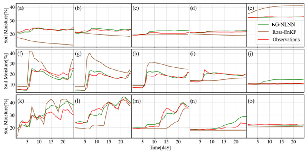
Figure B1 The 24 d predicted soil moisture time series of 5 depths with KG-NLNN and Ross-EnKF at Falkenberg (a–e), Cape-Charles (f–j), and Goodwell (k–o).

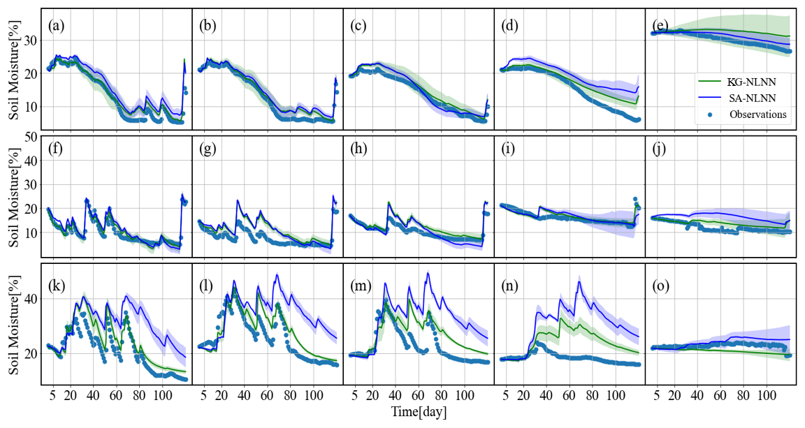
Figure B2 The 120 d predicted soil moisture time series of 5 depths with KG-NLNN and SA-NLNN at Falkenberg (a–e), Cape-Charles (f–j), and Goodwell (k–o).

Moreover, our machine learning approach exhibits autoregressive error accumulation in long-term soil moisture predictions – a limitation not observed in knowledge-based modeling. As demonstrated by the 120 d autoregressive forecasts (Fig. B2), while model uncertainty gradually accumulates with prediction time, it remains within acceptable bounds. Importantly, the knowledge-guided KG-NLNN model maintains significantly greater stability across the entire prediction horizon.

Appendix C

Table C1 The MAE [%] values for 1, 3, 7, and 15 d forecasts of LSTM_T LSTM_I, the proposed KG-NLNN and SA-NLNN model at 5 depths under four designed scenarios. The bold values indicate the best performance for each metric across the models.