Regionalization of IDF curves for mainland China: a comparative evaluation of machine learning versus spatial interpolation techniques

Regionalization of Intensity-Duration-Frequency (IDF) curves is essential for designing stormwater drainage systems, especially in regions without rainfall data of high temporal resolution. However, most studies have not thoroughly compared regionalization methods using sub-daily site observations versus gridded daily precipitation products. The potential of machine learning (ML) methods driven by daily gridded precipitation remains largely underexplored. This study addresses these gaps by regionalizing the IDF curves across mainland China for durations ranging between 1 and 72 h and return periods ranging from 2 to 1000 years. Five interpolation methods based on hourly observations from 2363 stations and five machine learning methods using a gridded daily dataset were tested for accuracy. Both ML and traditional interpolation methods showed robust performances based on the Kling-Gupta Efficiency (KGE) performance measure. The most successful interpolation method was Kriging with External Drift using mean annual precipitation, with KGE > 0.96 for 1 h–5-year and 24 h–5-year storms and KGE > 0.84 for 1 h–100-year and 24 h–100-year storms, while Gradient Boosting was the best-performing ML model, with KGE > 0.94 for 1 h–5-year and 24 h–5-year storms and KGE > 0.87 for 1 h–100-year and 24 h–100-year storms. Notably, even though ML used daily data and interpolation used hourly data, the ML accuracy gradually improved, eventually approaching or even surpassing the interpolation methods as the duration and return period increased. Consequently, a regionalized dataset on IDF curves for mainland China with a spatial resolution of 0.1° (and optionally 0.5°) was generated using the optimal regionalization method.

1 Introduction

The intensity and frequency of extreme precipitation are projected to increase under global warming in response to increased radiative forcing on the hydrologic cycle based on governing physical laws, including the Clausius-Clapeyron relationship (Benestad et al., 2021; Donat et al., 2016; Skliris et al., 2016). These extreme events can lead to disasters, including urban flooding, flash floods, and soil erosion, resulting in significant loss of life and property damage (Gao et al., 2017; Maggioni and Massari, 2019). Intensity-Duration-Frequency (IDF) curves, which define the relationships among rainfall intensity, duration, and frequency of occurrence (or the return period), are derived from historical extreme precipitation events. They play a vital role in the design of stormwater drainage systems and flood protection structures. In regions susceptible to severe flooding, accurately estimating IDF curves is crucial for developing infrastructure that can mitigate property damage and safeguard human lives (Simonović, 2012).

Extreme precipitation events are typically characterized by short duration, high intensity, and considerable spatial-temporal variability. As a result, developing accurate IDF curves requires station data with high spatial density and temporal resolution, such as hourly measurements (Förster and Thiele, 2020; Westra et al., 2014). However, the limited availability of observational stations with high temporal resolution means that IDF curves can only be derived for areas where such stations exist. Consequently, it is challenging to extend these curves to regions lacking high-resolution precipitation records (Sangüesa et al., 2023). With increased urbanization, many new water-related infrastructures will be built in areas without long-term historical precipitation data. Therefore, it is crucial to regionalize and estimate IDF curves for regions where high temporal resolution precipitation data is unavailable or limited.

Conventionally, regionalization relies on site-specific observations, with commonly used methods including Regional Frequency Analysis (RFA) and spatial interpolation (Szolgay et al., 2009). Regionalization of station IDFs through RFA requires identification of homogeneous regions (Schlef et al., 2023). However, this process can be challenging, as defining homogeneous regions often involves subjective judgment and lacks a solid physical basis (Nguyen et al., 2002). As a result, the regions identified may be heterogeneous, which can negatively impact frequency analysis (Halbert et al., 2016; Schlef et al., 2023). Additionally, boundary discontinuities between subregions present another challenge for RFA (Zou et al., 2021).

Regionalization methods for IDF curves derived from ground observations also involve interpolation. Two primary approaches are commonly used (Szolgay et al., 2009): (a) directly interpolating the quantiles, moments, or parameters of the distribution function, followed by the calculation of the distribution function for each region; or (b) first calculating the distribution function at the observation stations, then interpolating the return period estimates. Research conducted in the Haihe River Basin, China, for example, shows that interpolating return period estimates are more accurate compared to interpolation based on distribution parameters (Yin et al., 2018).

In terms of specific interpolation methods, researchers have frequently employed and compared methods such as Inverse Distance Weighting (IDW), Ordinary Kriging (OK), and Kriging with External Drift (KED). The KED method achieves higher accuracy by incorporating auxiliary variables correlated with the spatial distribution of the target variable (Berndt and Haberlandt, 2018; Shehu et al., 2023; Yin et al., 2018). For extreme rainfall prediction, auxiliary variables such as elevation and annual precipitation are correlated with the predicted variable and have the potential to improve interpolation accuracy (Miao et al., 2024; Zou et al., 2021). Notably, the accuracy of interpolation methods fundamentally depends on the quality of the observations. To generate reliable regionalized IDF curves requires a dense observational network with long-term, high-resolution data (Berndt et al., 2014; Papalexiou, 2018; Papalexiou and Koutsoyiannis, 2013; Shehu et al., 2023).

In recent years, gridded precipitation datasets have undergone significant improvements in both resolution and reliability, enhancing the potential for estimating IDF curves in regions where the deployment of observational stations is challenging (Courty et al., 2019). Consequently, the utilization of gridded precipitation datasets to develop IDF curves has become increasingly prevalent (Ghebreyesus and Sharif, 2021; Mínguez and Herrera, 2023; Noor et al., 2021). These datasets can be generated through various methods, including ground-based station observations, radar, satellite data, or a combination of these sources, resulting in precipitation datasets with varying temporal and spatial resolutions, from which gridded IDF products can be estimated (Haruna et al., 2024; Lanciotti et al., 2022; Wambura, 2024). However, estimating IDF curves involves assessing precipitation extremes, which may exhibit strong spatial heterogeneity within individual grid cells of precipitation datasets. Further improvements are necessary to enhance the accuracy of gridded IDF products derived from such datasets (Parding et al., 2023; Schilcher et al., 2017).

Recent studies have explored the application of machine learning methods for regionalizing IDF curves. Several studies have successfully trained machine learning models on sub-daily precipitation data. For example, one study utilized Support Vector Machine to create a gridded IDF dataset for Canada, while another established a gridded IDF dataset for the Qinghai-Tibet Plateau using Random Forest model (Gaur et al., 2020; Ren et al., 2025). Concurrently, other researches have investigated the non-stationarity of IDF curves under changing climate conditions (Schlef et al., 2023; Vinod and Mahesha, 2024; Zhang et al., 2022). A key challenge in this context is temporal downscaling, where some researches have employed machine learning to disaggregate coarse 3 h precipitation outputs from climate models into minute-level resolution (Al Kajbaf et al., 2022, 2023). This demonstrates the potential of machine learning methods to produce gridded IDF datasets, which traditionally requires sub-daily data, by utilizing precipitation data of a coarser temporal resolution (e.g., daily observations common to rain gauges).

The different advantages and disadvantages of the aforementioned IDF curves regionalization methods indicate that it is necessary to identify an optimal regionalization method based on comparative analysis. However, most existing studies assess the accuracy of regionalized IDF curves based on either site-specific observations or grid-based datasets, without comparing these two kinds of regionalization methods. Additionally, few studies have evaluated the potential of applying machine learning to daily gridded precipitation datasets for estimating regionalized IDF curves, including extrapolation to rainfall intensities at sub-daily time intervals. Furthermore, few studies have computed regionalized IDF curves on a national scale in China.

To address these gaps and advance IDF regionalization, this paper is structured as follows. Section 2 describes the study area, data sources, and methods, including the development of IDF curves, spatial interpolation techniques, machine learning approaches, and evaluation metrics. Section 3 presents the results, covering station-level IDF characteristics, a comparative evaluation of regionalization methods at national and regional scales, and the final regionalized IDF curves. Section 4 discusses the implications of the findings, limitation of the final IDF datasets, and opportunities for improvement. Finally, Sect. 5 summarizes the key conclusions and contributions of the study.

2 Data and Methods

2.1 Study area and data collection

The study focused on the regionalization of IDF curves on a national scale in mainland China. However, a method that performs well at the national level may exhibit poor accuracy in specific regions. To address this, this study adopted a regionalization scheme that divides mainland China into three distinct regions: the Southwestern Tibetan Plateau (SW) region, the Northwestern Arid (NW) region, and the Eastern Monsoon region(Wang et al., 2019; Zhao, 1983). Due to substantial internal heterogeneity within the Eastern Monsoon region, it was further divided into the Northeastern Monsoon (NE) sub-region and Southeastern Monsoon (SE) sub-region along the Qinling-Huaihe line (Fig. 1). This division reflects significant regional differences in climate and topography. To provide additional regional perspective, we also evaluated model performance using an alternative division scheme based on the nine major river basins of China (Fig. S3 and Tables S23 to S30 in the Supplement).

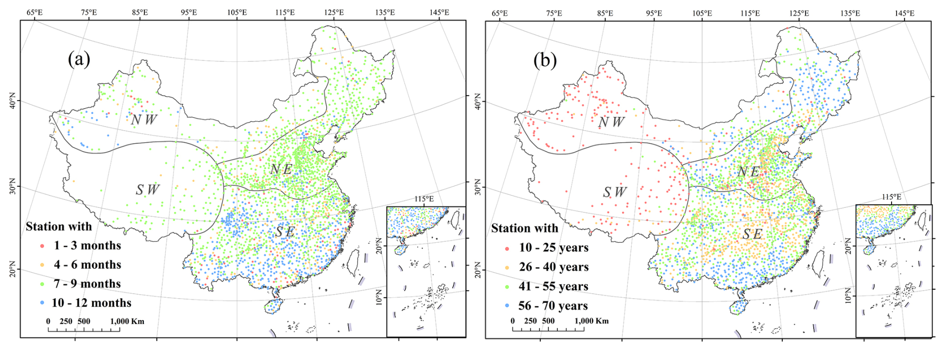
Figure 1 The spatial distribution of 2363 stations with hourly observations for this study, showing (a) the number of operational months per year, and (b) record lengths. The inset displays the South China Sea Islands within the nine-dash line.

To regionalize IDF curves across mainland China, this study utilized two datasets: hourly observations from 2363 stations in mainland China and gridded daily data from the CHM_PRE (Han et al., 2023). The hourly observations were provided and quality-controlled by the National Meteorological Information Center (NMIC) of the China Meteorological Administration (CMA) (Li et al., 2011). Hourly data were observed by siphon self-recording rain gauges, which were not operational during the cold season in some regions to prevent instrument failures caused by low temperatures. The number of operational months for each station is shown in Fig. 1a. Additional quality control measures were applied to ensure the reliability of the hourly observations used in developing the IDF curves. Stations were included if they had less than 10 % missing data per year. Besides, to ensure a robust sample size for fitting the GEV distribution, only stations with at least 10 years of precipitation records were retained (Ren et al., 2025). Consequently, the data record for the selected stations span from 1951 to 2020, with record lengths ranging from 10 to 70 years, as shown in Fig. 1b. To address missing data and prevent underestimation, gaps were handled as follows: (1) for missing periods less than 12 h, the recorded hourly data were linearly interpolated; (2) for continuous gaps of 12 h or longer, no interpolation was attempted, and the hours with missing data were assigned a value of zero. From these quality-controlled hourly observations, 27 extreme hourly indices were extracted. Specifically, the annual maximum rainfall for durations from 1 to 24 h by 1 h increments, as well as longer durations of 36, 48, and 72 h, were identified on a yearly basis using a moving window method, resulting in an annual maximum series for each location.

The CHM_PRE dataset is a high-quality gridded precipitation dataset covering mainland China. The daily dataset spans the period from 1961 to 2022, with multiple spatial resolutions (0.1°×0.1°, 0.25°×0.25°, and 0.5°×0.5°). It is constructed using daily observations from 2839 gauges across China and nearby regions, employing an interpolation scheme that combines the Parameter-elevation Regression on Independent Slopes Model (PRISM) for the daily climatology field with inverse-distance weighting to interpolate station observations into the ratio field (Han et al., 2023). In this study, 0.1°×0.1° CHM_PRE was selected. CHM_PRE served as the primary independent variable for the machine learning methods, providing essential input for regionalizing IDF curves across mainland China. Since the dependent variable was based on hourly observations, utilizing independent variables derived from such daily observations did not pose a risk of data leakage. In addition to CHM_PRE, we also explored the CGDPP (Shen et al., 2010) and CHIRPS (Funk et al., 2015) datasets (Tables S1 to S12). However, since they did not demonstrate better performance compared to CHM_PRE, they were not selected for this study.

2.2 Development of IDF curves

The construction of Intensity-Duration-Frequency (IDF) curves in this study follows the Koutsoyiannis method, which calculates generalized rainfall intensity as a function of duration (Koutsoyiannis et al., 1998). Specifically, the generalized intensity i is formulated as:

$$\begin{array}{}\text{(1)}& i=i_d\cdot b_d\end{array}$$

Here, d denotes the duration in hours, and i_d is the intensity calculated by using the annual maximum series (AMS) method for each duration. The function b_d is:

$$\begin{array}{}\text{(2)}& b_d={\left(d+\mathit{\theta }\right)}^{\mathit{\eta }}\end{array}$$

where the parameters θ and η are estimated for each station by minimizing the Kruskal–Wallis statistic (Koutsoyiannis et al., 1998). Having estimated θ and η, the generalized intensities are pooled together under the assumption that they follow the same distribution for all durations. For the distribution fitting process, this study employs the Generalized Extreme Value (GEV) distribution. The GEV distribution function (Jenkinson, 1955) can be expressed as:

$$\begin{array}{}\text{(3)}& \begin{array}{rl}G\left(z;\mathit{\mu },\mathit{\sigma },\mathit{\xi }\right)& =\exp \left\{-{\left[\mathrm{1}+\mathit{\xi }\left({\displaystyle \frac{z-\mathit{\mu }}{\mathit{\sigma }}}\right)\right]}^{-\mathrm{1}/\mathit{\xi }}\right\},\mathrm{1}\\ & +{\displaystyle \frac{\mathit{\xi }\left(z-\mathit{\mu }\right)}{\mathit{\sigma }}}>\mathrm{0},\mathit{\xi }\ne \mathrm{0}\end{array}\end{array}$$

where μ is the location parameter, σ is the scale parameter, and ξ is the shape parameter. These parameters can be estimated with the L-moment method (Hosking, 1990). Once the GEV parameters were determined, the corresponding $\left(\mathrm{1}-r^{-\mathrm{1}}\right)$th quantile of the GEV distribution for a r-year return period could be calculated. The IDF curves are finally generated by estimating quantiles at specific return periods from the fitted GEV distribution and dividing these quantiles by the term b_d. In this study, the durations selected were whole hours from 1 to 24, along with 36, 48, and 72 h, and the return periods were 2, 5, 10, 20, 50, 100, 200, 500, and 1000 years.

2.3 The spatial interpolation methods

Traditional spatial interpolation methods were used in this study to regionalize IDF curves. Both deterministic interpolation and geostatistical interpolation methods were utilized. Inverse Distance Weighted (IDW) represents a deterministic interpolation method, while Kriging is a form of geostatistical interpolation.

The fundamental principle of IDW is that the influence of a known point diminishes with increasing distance from the unknown point. Mathematically, the estimated value Z(x₀) at location x₀ is calculated as follows:

$$\begin{array}{}\text{(4)}& Z\left(x_{\mathrm{0}}\right)={\displaystyle \frac{{\sum }_{i=\mathrm{1}}^n\frac{Z\left(x_i\right)}{d{\left(x_i,x_{\mathrm{0}}\right)}^p}}{\sum _{i=\mathrm{1}}^n\frac{\mathrm{1}}{d{\left(x_i,x_{\mathrm{0}}\right)}^p}}}\end{array}$$

where Z(x_i) represents the known value at location x_i, d(x_i,x₀) is the Euclidian distance between the known point x_i and the unknown point x₀, p is the power parameter that controls the rate of decay of influence with distance, and n is the number of known points used in the interpolation. In this study, the IDW method was implemented using a power parameter p of 2, which is a commonly used value that provides a balance between smoothness and accuracy (Li and Heap, 2008).

Kriging interpolation is a geostatistical method that assumes a stochastic process with spatial correlation between different points. The core of Kriging interpolation lies in the calculation of the variogram, which represents the spatial correlation between points at different distances. Initially, various lag distances are defined, and the semi-variance of residuals at these lag distances is calculated to generate the empirical variogram. The formula for the semi-variance (Armstrong, 1998) is as follows:

$$\begin{array}{}\text{(5)}& \mathit{\gamma }\left(h\right)={\displaystyle \frac{\mathrm{1}}{\mathrm{2}N\left(h\right)}}{\sum }_{i=\mathrm{1}}^{N\left(h\right)}{\left[Z\left(x_i\right)-Z\left(x_i+h\right)\right]}^{\mathrm{2}}\end{array}$$

where γ(h) is the semivariance at lag distance h, N(h) is the number of pairs of points separated by h, Z(x_i) is the value at location x_i, and Z(x_i+h) is the value at location x_i+h. Subsequently, a theoretical model is fitted to the empirical variogram. In this study, the commonly used spherical model was employed.

Ordinary Kriging (OK) assumes that the trend is an unknown constant. The formula (Verworn and Haberlandt, 2011) for Ordinary Kriging is:

$$\begin{array}{}\text{(6)}& \widehat{Z}\left(x_{\mathrm{0}}\right)={\sum }_{i=\mathrm{1}}^n{\mathit{\lambda }}_{i}Z\left(x_i\right)\end{array}$$

where $\widehat{Z}\left(x_{\mathrm{0}}\right)$ is the estimated value at location x₀, λ_i are the weights, and Z(x_i) are the known values at locations x_i. The weights are determined using the Kriging equations based on the variogram.

Kriging with External Drift (KED) incorporates one or more auxiliary variables as background information for the interpolation of the primary variable. KED assumes that the expectation of the primary variable is a linear combination of these auxiliary variables (Verworn and Haberlandt, 2011):

$$\begin{array}{}\text{(7)}& E\left[Z\right(x\left)\right|Y_{\mathrm{1}}\left(x\right),Y_{\mathrm{2}}\left(x\right),\mathrm{\dots },Y_m\left(x\right)]={\mathit{\beta }}_{\mathrm{0}}+{\sum }_{k=\mathrm{1}}^m{\mathit{\beta }}_k{Y}_k(x)\end{array}$$

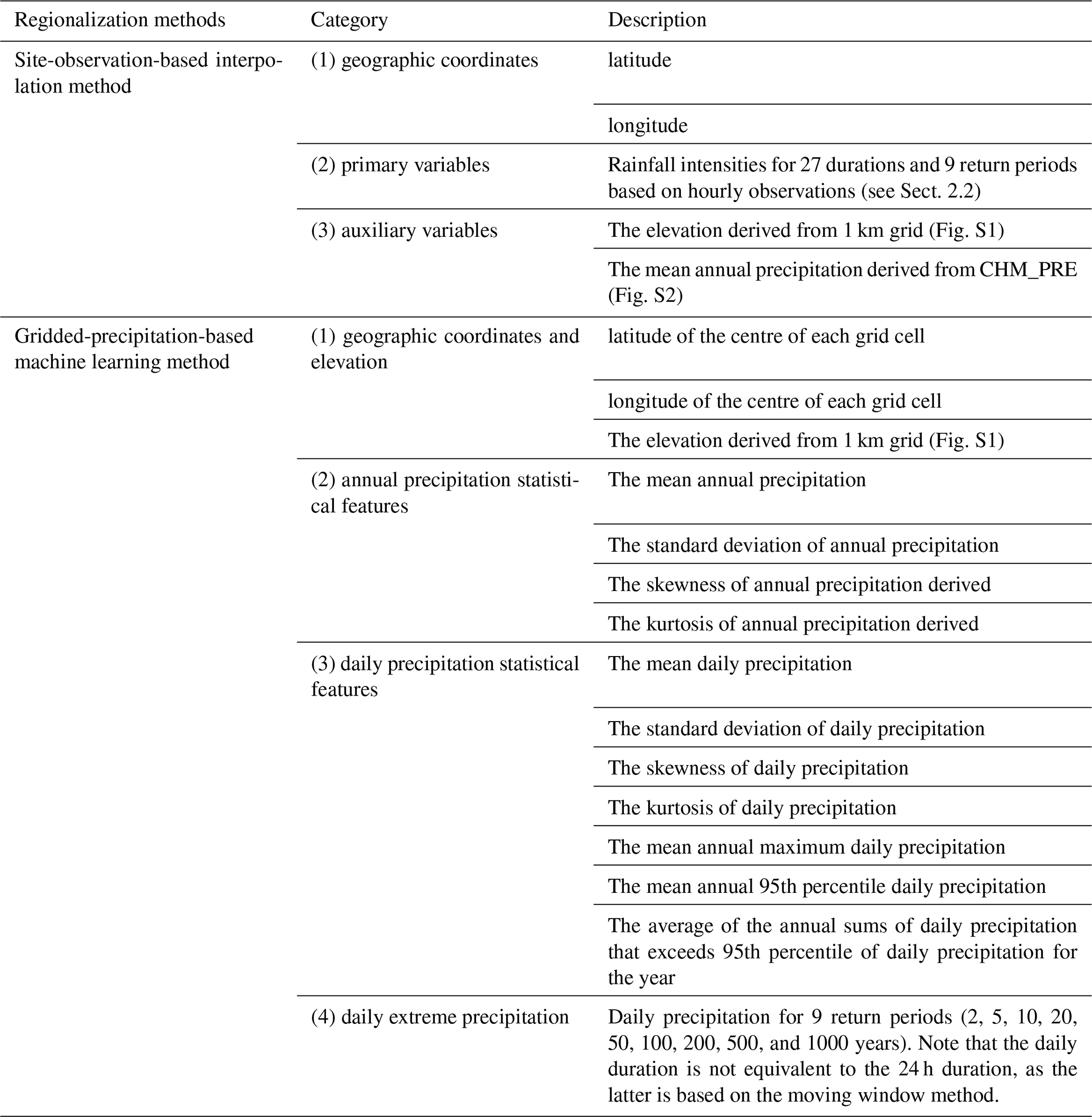
where $E\left[Z\right(x\left)\right|Y_{\mathrm{1}}\left(x\right),Y_{\mathrm{2}}\left(x\right),\mathrm{\dots },Y_m\left(x\right)]$ is the expectation of the primary variable at location x, ${\mathit{\beta }}_{\mathrm{0}},{\mathit{\beta }}_{\mathrm{1}},\mathrm{\dots },{\mathit{\beta }}_m$ are the unknown constants, and $Y_{\mathrm{1}}\left(x\right),Y_{\mathrm{2}}\left(x\right),\mathrm{\dots },Y_m\left(x\right)$ are the auxiliary variables. It is important to note that when calculating the variogram using the KED method, $E\left[Z\right(x\left)\right|Y_{\mathrm{1}}\left(x\right),Y_{\mathrm{2}}\left(x\right),\mathrm{\dots },Y_m\left(x\right)]$ at different spatial points vary. Therefore, the residuals must be calculated first, and then the semi-variance based on residuals is computed. The residuals are calculated as: $R\left(x\right)=Z\left(x\right)-E\left[Z\left(x\right)\right]$. In this study, annual precipitation and elevation were used as auxiliary variables (Table 1). The spatial resolution of the annual precipitation data and the elevation data were both 1 km × 1 km. The interpolation methods were all performed using the “gstat” package in R (Pebesma, 2004).

Table 1 Independent variables used in the regionalization methods evaluated. The gridded precipitation data are sourced from CHM_PRE.

2.4 Machine learning methods

In this study, machine learning methods were applied using the scikit-learn (sklearn) library in Python (Pedregosa et al., 2011), taking advantage of the CHM_PRE dataset (see Sect. 2.1). For each grid cell, we first calculated a set of independent variables, grouped into four categories: geographic coordinates and elevation, statistics of annual and daily precipitation, and daily extreme precipitation for different return periods (Table 1). These selected and readily available independent variables without introducing additional meteorological variables allow testing the predictive potential inherent within the precipitation data, while also ensuring the method's practicality and applicability, particularly in regions where other high-quality meteorological data are limited or unavailable. We then aligned each observational station to the grid cell in which the station is located, and treated the station-derived rainfall intensity at specific duration and frequency as dependent target variables. The datasets used to evaluate prediction accuracy were based on all grids that contained both independent and dependent variables.

Then a range of four general test cases were extracted from the IDF curves that, for simplicity, are referred to herein as the short duration-small return period (SDSR), short duration-large return period (SDLR), long duration-small return period (LDSR), and long duration-large return period (LDLR) cases, corresponding to the four permutations of IDF cases with 1 and 24 h durations, and 5 and 100-year return periods. These targets were selected to represent varying durations and return periods, thereby capturing the different scales of extremes within the IDF framework. These selected cases were used to evaluate the performance of the different regionalization methods.

To predict extreme rainfall intensities, 10 different machine learning methods (Table S13) were considered initially, and cross-validation was used to evaluate their accuracy. For each case, we calculated performance scores according to the procedure described in Sect. 2.5. The five highest-scoring machine learning methods, based on the average scores across all the four cases, were Random Forest (RF), Gradient Boosting (GB), Extremely Randomized Trees (ET), Multilayer Perceptron (MLP), and Linear Regression (LR) (Breiman, 2001; Friedman, 2001; Geurts et al., 2006; Hinton, 1989).

It should be noted that we also performed hyperparameter tuning using a grid search for each model for the four cases (Tables S14 to S17). However, the best performance among all machine learning methods with tuned hyperparameters did not show a significant improvement over that with the default settings provided by the Scikit-learn library. Additional experiments using Bayesian optimization (Mockus et al., 1978; Snoek et al., 2012) to search for optimal hyperparameters also failed to yield notable improvement (Tables S18 to S22). Consequently, for simplicity and consistency, we proceeded with the default hyperparameters throughout the study.

2.5 Evaluation of the regionalization efficiency

This study employed five-fold cross-validation to evaluate the prediction accuracy of interpolation and machine learning methods. Additionally, cross-validation helps mitigate the risk of overfitting, ensuring more robust and generalizable results. In each iteration, 80 % of the data was used to train the model, while the remaining 20 % was reserved for validation. This process was repeated five times using sampling without replacement, ensuring that each data point was used for validation exactly once. The predicted values were then compared with the observations to evaluate accuracy using the following metrics: Nash-Sutcliffe Efficiency (NSE), Percent Bias (PBIAS), Root Mean Square Error (RMSE), and Kling-Gupta Efficiency (KGE). The formulas for these evaluation metrics are provided below:

$$\begin{array}{}\text{(8)}& {\displaystyle }\mathrm{NSE}=\mathrm{1}-{\displaystyle \frac{{\sum }_{i=\mathrm{1}}^n{\left(O_i-P_i\right)}^{\mathrm{2}}}{{\sum }_{i=\mathrm{1}}^n{\left(O_i-\stackrel{\mathrm{‾}}{O}\right)}^{\mathrm{2}}}}\text{(9)}& {\displaystyle }\mathrm{PBIAS}=\mathrm{100}\mathit{\%}\times {\displaystyle \frac{{\sum }_{i=\mathrm{1}}^n\left(P_i-O_i\right)}{{\sum }_{i=\mathrm{1}}^n{O}_i}}\text{(10)}& {\displaystyle }\mathrm{RMSE}=\sqrt{{\displaystyle \frac{{\sum }_{i=\mathrm{1}}^n{\left(P_i-O_i\right)}^{\mathrm{2}}}{n}}}\text{(11)}& {\displaystyle }\mathrm{KGE}=\mathrm{1}-\sqrt{{\left(\mathrm{CC}-\mathrm{1}\right)}^{\mathrm{2}}+{\left({\displaystyle \frac{{\mathit{\sigma }}_P/\stackrel{\mathrm{‾}}{P}}{{\mathit{\sigma }}_O/\stackrel{\mathrm{‾}}{O}}}-\mathrm{1}\right)}^{\mathrm{2}}+{\left({\displaystyle \frac{\stackrel{\mathrm{‾}}{P}}{\stackrel{\mathrm{‾}}{O}}}-\mathrm{1}\right)}^{\mathrm{2}}}\end{array}$$

where O_i denotes the observed values, P_i denotes the predicted values. Specifically, O_i is the extreme rainfall intensity for a given duration and return period estimated from hourly data at an individual site, while P_i is the corresponding value for that site predicted by a model (either interpolation or machine learning) trained on data that excluded the site being evaluated. $\stackrel{\mathrm{‾}}{O}$ and $\stackrel{\mathrm{‾}}{P}$ are the mean of the observed and the predicted values, respectively. σ_O and σ_P are the standard deviations of the observed and predicted values, respectively. CC is the Pearson correlation coefficient:

$$\begin{array}{}\text{(12)}& \mathrm{CC}={\displaystyle \frac{{\sum }_{i=\mathrm{1}}^n\left(P_i-\stackrel{\mathrm{‾}}{P}\right)\left(O_i-\stackrel{\mathrm{‾}}{O}\right)}{\sqrt{{\sum }_{i=\mathrm{1}}^n{\left(P_i-\stackrel{\mathrm{‾}}{P}\right)}^{\mathrm{2}}}\sqrt{{\sum }_{i=\mathrm{1}}^n{\left(O_i-\stackrel{\mathrm{‾}}{O}\right)}^{\mathrm{2}}}}}\end{array}$$

The maximum value for NSE is 1, with higher values indicating better predictive performance. PBIAS values indicate overestimation (positive) or underestimation (negative), with lower absolute values representing smaller prediction errors. RMSE has a minimum value of 0, where smaller values denote less error. KGE reflects the correlation, variability, and bias between predicted and observed values, with its maximum value being 1 and higher values indicating better performance.

To determine the optimal regionalization method for each specific duration and return period, a weighted composite score based on the above four metrics was defined. First, each metric was individually standardized using standard deviation normalization among all methods (mean of 0, with positive or negative values indicating above or below the mean, respectively, and the values representing multiples of the standard deviation from the mean). The standardized metrics were then weighted and averaged to calculate the final score for each method using assigned weights of 0.2, 0.2, 0.2, and 0.4, respectively (RMSE's standardized values were negated, and PBIAS values were first converted to absolute values before negation). The method with the highest weighted composite score was selected as the optimal regionalization method for the given duration and return period. This selection process was performed for the permutations of 27 durations and 9 return periods ($\mathrm{27}\times \mathrm{9}=$ 243 times). The selected optimal regionalization method was then applied to regionalize extreme rainfall intensity for each specific duration and return period.

3 Results

3.1 Station-level IDF curves in Mainland China

To establish a foundation for regionalizing IDF curves, we first analyzed station-level IDF curves derived from the observed rainfall data across the NMIC ground network. These station-specific IDF curves, serving as the dependent variable in subsequent analyses, provide the most accurate representation of extreme rainfall intensities (Fig. 2). The specific statistical characteristics of the four IDF cases used to test regionalization methods are summarized in Table S49. The mean values clearly highlight differences in the magnitude of rainfall intensity across the cases. The LDSR exhibits a mean intensity of 4.5 mm h⁻¹, whereas the LDLR shows a significantly higher mean intensity of 8.42 mm h⁻¹, indicating higher rainfall intensity. This pattern of increasing rainfall intensity with larger return periods is evident for both short and long durations. In addition, the mean intensity for shorter durations, such as the SDLR (76.38 mm h⁻¹), is much higher compared to longer durations like the LDLR. These results emphasize the variations in IDF curves: shorter durations and larger return periods correspond to higher rainfall intensities, underscoring the increasing severity, which can also be inferred to in Sect. 2.2. Such rainfall intensity of shorter durations and larger return periods may pose additional challenges for accurate prediction.

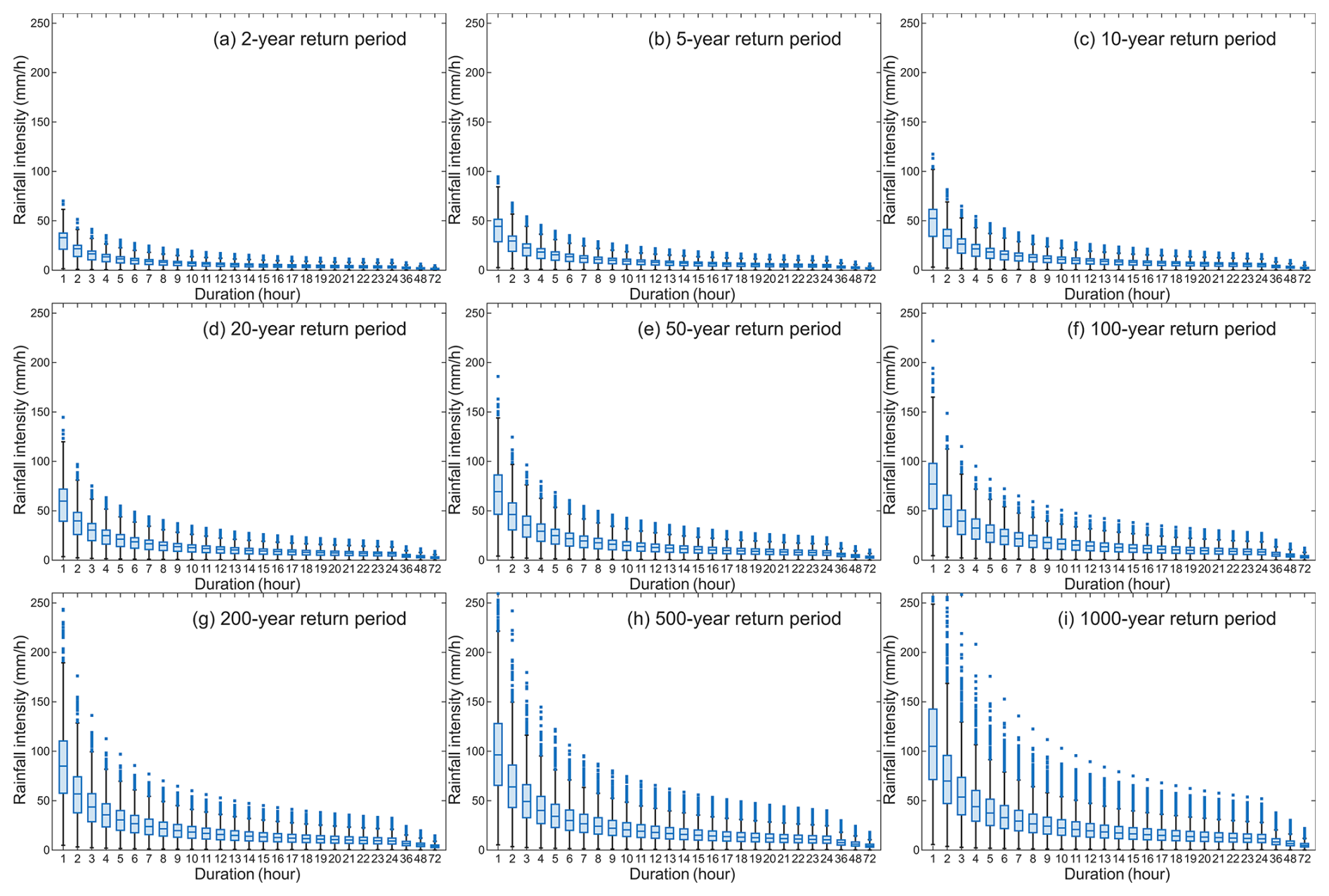
Figure 2 Boxplots of observed station-level rainfall intensities for various durations and return periods across stations in mainland China.

3.2 Evaluation of regionalization method types

To evaluate the performance and reliability of different methods for regionalizing IDF curves across mainland China, this study systematically compares five traditional interpolation methods and five machine learning methods. The objective is to assess the predictive capabilities of these methods, explore the potential of machine learning methods for regionalizing IDF curves, and demonstrate the reliability of the regionalized IDF curves product created by applying the optimal method (selected from the ten evaluated methods) to each of the four IDF cases with a specific duration and return period combination.

3.2.1 Interpolation methods

Prediction accuracy for the five interpolation methods and five machine learning methods across four cases are presented in Tables 2 and 3, respectively. The weighted composite scores derived from these metrics are shown in Fig. 3. Among the interpolation methods, Inverse Distance Weighting (IDW), a deterministic interpolation technique, consistently underperformed compared to the geostatistical models represented by the Kriging methods (Fig. 3). This performance gap was particularly evident for cases with smaller return periods. As shown in Table 2, IDW exhibited inferior performance relative to the Kriging methods across almost all performance metrics for cases with smaller return periods.

Table 2 Accuracy metrics of interpolation methods in mainland China.

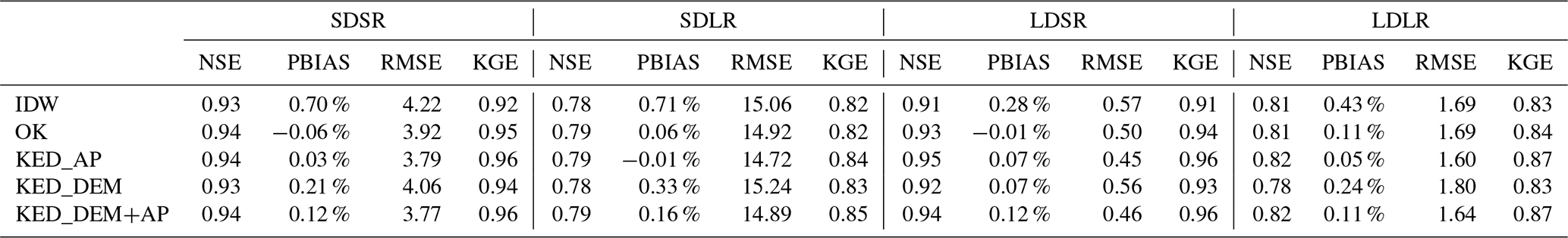
NSE and KGE are dimensionless and RMSE is in mm h⁻¹. Positive (negative) PBIAS (in percentage) indicates overestimation (underestimation).

Table 3 Accuracy metrics of machine learning methods in mainland China.

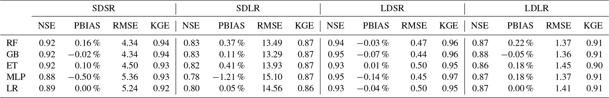
NSE and KGE are dimensionless and RMSE is in mm h⁻¹. Positive (negative) PBIAS (in percentage) indicates overestimation (underestimation).

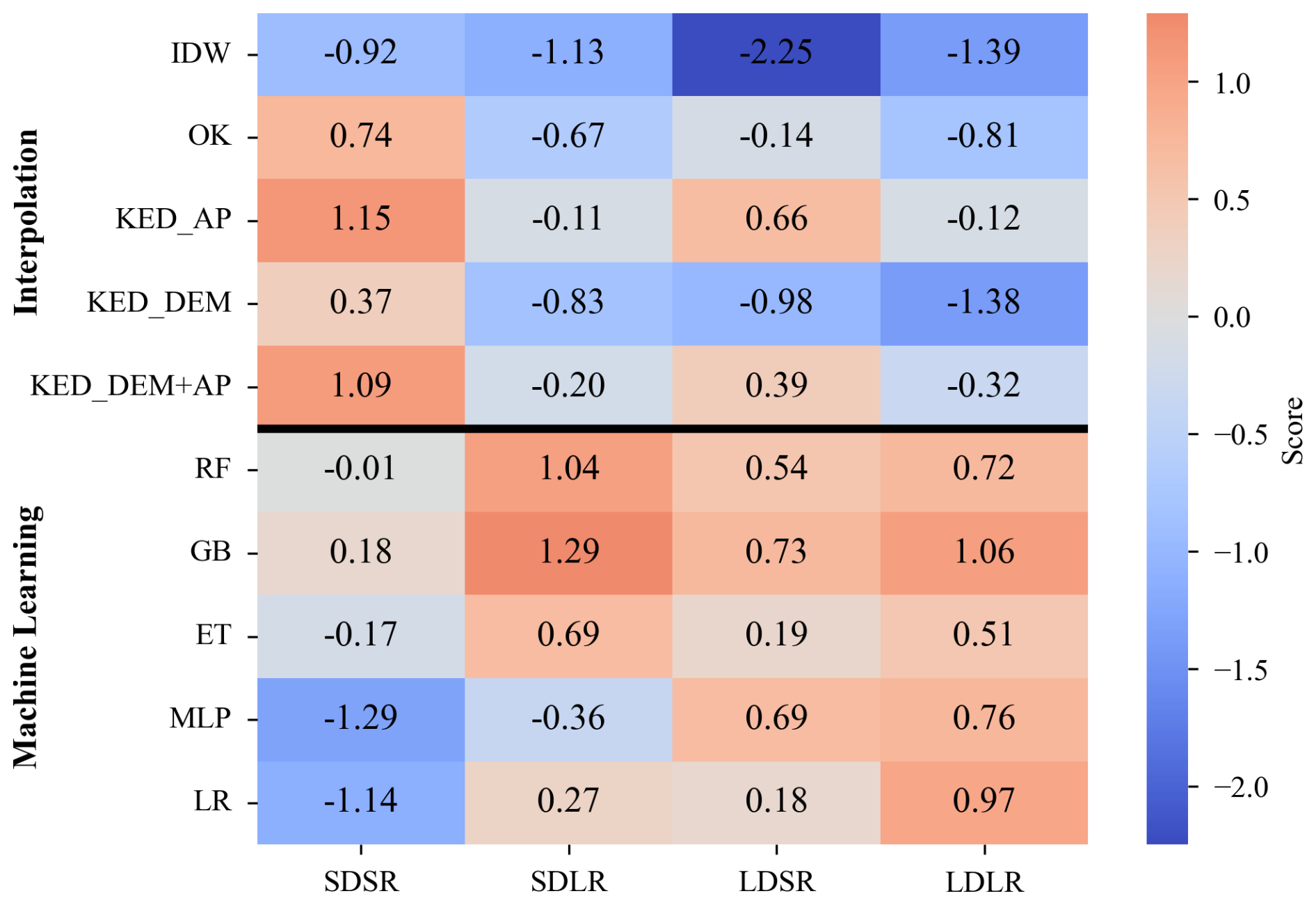
Figure 3 Weighted composite scores of all regionalization methods. Larger, more positive values represent better performance, with a value of 0 representing average performance.

Among the four Kriging methods, Kriging with External Drift using annual average precipitation (KED_AP) demonstrated improved scores across all four cases compared to Ordinary Kriging (OK) which does not incorporate covariates (Fig. 3). However, when elevation was used as a covariate (KED_DEM), scores declined for all the four cases. Similarly, when both annual precipitation and elevation were included as covariates (KED_DEM+AP), the pattern remained consistent with KED_DEM, showing decreased scores for all the four cases compared to KED_AP (Fig. 3). These trends were further corroborated in terms of NSE, PBIAS, RMSE, and KGE presented in Table 2, which are largely aligned with the observed score patterns.

These results indicate that IDW is less effective at predicting extreme rainfall intensities compared to Kriging methods across the four cases. Among the Kriging methods, incorporating annual precipitation as a covariate significantly improved prediction accuracy, whereas including elevation as a covariate did not, and in some cases, even with reduced accuracy. This finding is consistent with previous studies conducted in the Haihe River Basin, China (Zou et al., 2021).

3.2.2 Machine learning methods

As shown in Fig. 3, among the five machine learning methods, Gradient Boosting (GB) performed the best, achieving the highest scores for all cases. In the final regionalized IDF curves, GB also outperformed the other methods and became the optimal method in many cases (Table S31). Following GB's performance, both Random Forest (RF) and Extremely Randomized Trees (ET) demonstrated relatively stable performance across the four cases, showing acceptable scores with relatively small variability. In contrast, MLP and Linear Regression (LR) exhibited greater performance variability across the four cases (Fig. 3). For instance, while MLP achieved high scores for longer durations, its accuracy for shorter durations was notably lower, as indicated by the lower NSE and higher RMSE and PBIAS values (Table 3). However, the strength of MLP's accuracy in longer-duration cases allowed it to surpass GB and become the optimal method in certain longer-duration cases within the final regionalized IDF curves (Table S31).

3.2.3 Comparison between interpolation and machine learning methods

When comparing interpolation and machine learning methods, the highest composite scores for SDSR, SDLR, LDSR, and LDLR were achieved with KED_AP, GB, GB, and GB, respectively (Fig. 3). Notably, the difference in relative scores between the best interpolation and machine learning methods indicate that the performance gap narrows – and may even reverse – as the duration and return period increase (e.g., the score difference is 0.97 for SDSR and −1.18 for LDLR). This trend indicates that machine learning methods tend to perform better as the duration and return period increase. This observation is further supported by the final IDF curves dataset (Table S31). Furthermore, as shown in Tables 2 and 3, the expectation noted in Sect. 3.1 is confirmed: shorter duration and larger return periods are usually associated with increased prediction difficulty and reduced accuracy.

Methods with the highest scores from both interpolation and machine learning methods demonstrated strong performance across the four cases. For the most challenging case, SDLR, the highest scoring methods – KED_AP from the interpolation techniques and GB from the machine learning models – achieved KGE values not less than 0.84. For SDSR, LDSR, and LDLR, the highest scoring methods from both interpolation and machine learning methods produced KGE values of at least 0.94, 0.96, and 0.87, respectively, with PBIAS values close to zero, indicating little systematic bias (Tables 2 and 3).

In the subsequent sections, this study focuses on KED_AP and GB, which consistently demonstrated strong and stable performance across the four cases, as representative examples of interpolation and machine learning methods, respectively. These two methods are used to show the predictive results at various stations, highlighting both the potential of interpolation and machine learning methods for IDF regionalization and the regional variations in performance.

Figure 4 presents the prediction results from both interpolation and machine learning. For all four cases, estimated extreme rainfall intensities are generally aligned along the 1:1 line. In terms of distribution, the scatter points for the two cases with smaller return periods are more closely concentrated around the 1:1 line, while those for larger return periods exhibit greater dispersion (Fig. 4). In addition, analysis of relative errors (Fig. S5) reveals comparable performance between the two methods across all cases. The relative errors are notably smaller for smaller return periods (median RE: 0.39 %–0.65 %) compared to larger return periods (median RE: 1.5 %–2.5 %), indicating increased prediction uncertainty for more extreme events.

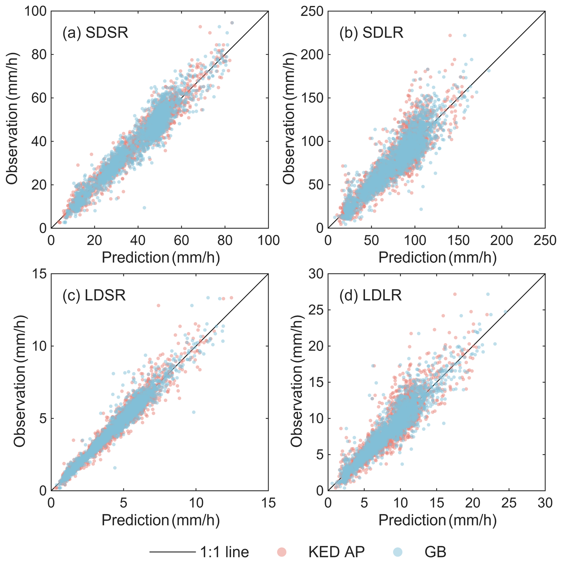
Figure 4 Scatterplots of observations and predictions for KED_AP (the best interpolation method) and GB (the best machine learning method).

The residuals (calculated as the difference between predicted and observed values) for both methods mostly show distributions that are close to be normally distributed (Fig. S6). However, compared to the true normal distribution, the residual distributions still exhibit mild negative skewness and higher kurtosis, suggesting that both methods tend to underestimate certain extreme values. These underestimation is evident in Fig. 4, where the corresponding values are scattered above the 1:1 line. For an ideal model, the residuals should be randomly distributed across the study area, with no obvious spatial patterns influenced by location or the magnitude of observed values. The spatial distribution of residuals is illustrated in Fig. 5. The overall spatial distribution of residuals is relatively random, with no obvious clustering or trend. Consistent with the findings from Fig. S6, there are marginally more instances of severe underestimation than severe overestimation across all cases. The above results of residual analysis also indicate that the predictive performance of interpolation and machine learning is satisfactory, with both providing reliable predictions across mainland China.

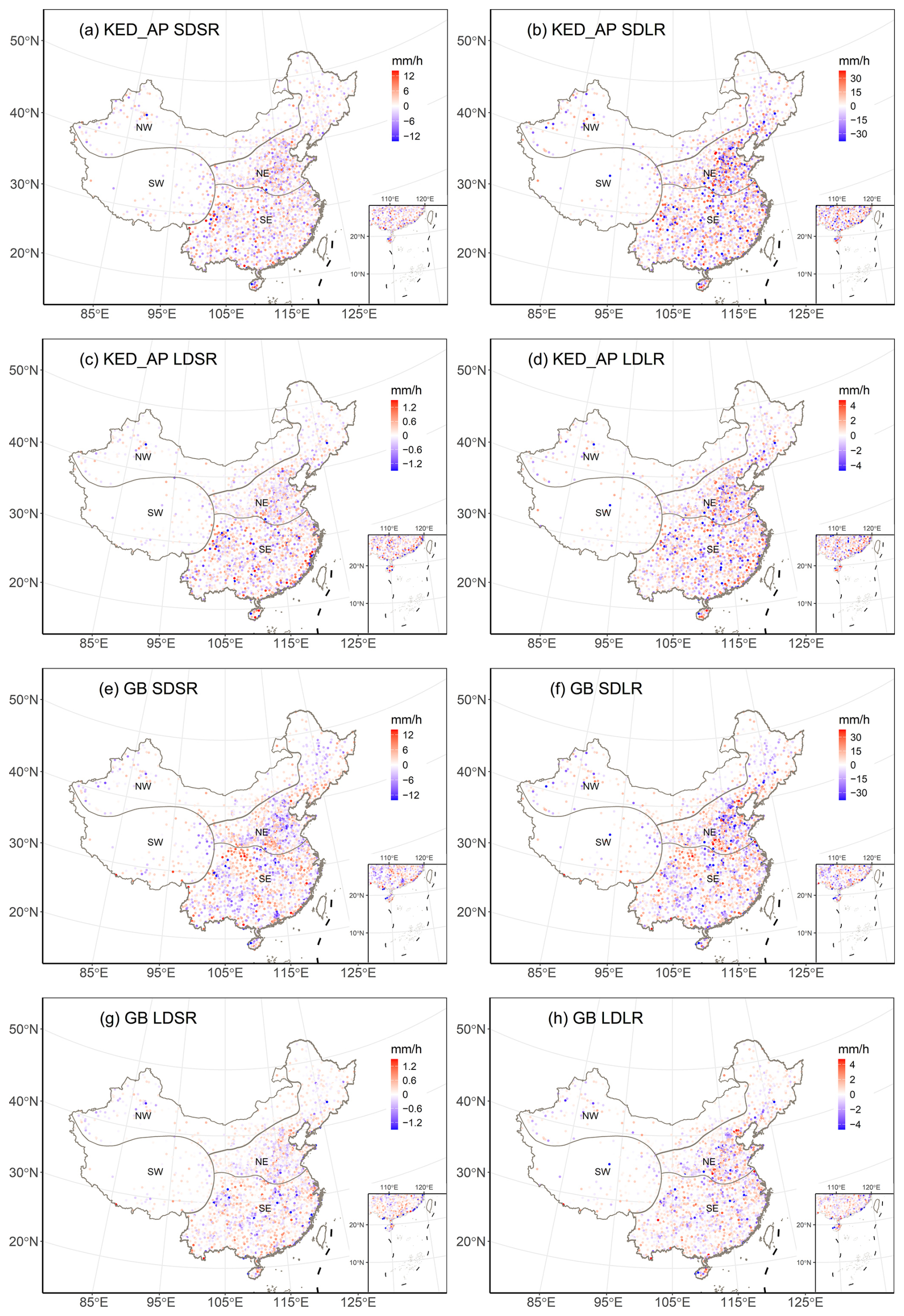
Figure 5 Spatial distribution of the residuals for KED_AP (the best interpolation method, a–d) and GB (the best machine learning method, e–h). Blue points represent underestimation, while red points represent overestimation.

In short, both interpolation and machine learning methods demonstrate comparable and robust performance across various cases, whether for short or long durations and return periods. This consistent accuracy in terms of accuracy metrics, residuals, and relative errors highlights the strong potential of the two methods for the regionalization of IDF curves in mainland China. Notably, machine learning, as a method not previously applied to IDF curves regionalization in mainland China, demonstrates accuracy comparable to traditional interpolation methods and even outperforms them in predicting cases for long durations and large return periods. Additionally, machine learning offers distinct advantages, such as requiring only daily precipitation data for regionalization once a model is trained (in contrast with interpolation methods, which always require known sub-daily level target values). Furthermore, machine learning is independent of station setup conditions, and possesses strong adaptability for future updates, forecasting, and climate projection. These features suggest that machine learning has the potential to replace interpolation methods in future IDF curves regionalization applications.

3.3 Regional performance evaluation of interpolation and machine learning methods

A method that performs well at the national level may exhibit poor accuracy for specific regions. To address this, this study adopted a regionalization scheme that divides mainland China into four regions (see Sect. 2.1). Using this scheme, we conducted a regional assessment across mainland China, using KED_AP and GB as representatives of interpolation and machine learning methods, respectively, to explore their applicability in the four distinct regions. Notably, we did not retrain the models for regional scales but used the nationally trained models to compute accuracy metrics within each region.

As an interpolation method, the predictive accuracy of KED_AP is influenced by station density and whether the interpolation assumptions, such as decreasing correlation with distance, are satisfied. In the NE region, where station density is high and precipitation patterns are relatively stable, KED_AP achieves high predictive accuracy, with a KGE of 0.94 for SDSR and LDSR (Table 4). In contrast, in the SE region, characterized by a humid subtropical and monsoon climate, the performance of KED_AP declines for SDSR, SDLR, and LDSR compared to the NE region, despite the dense station network (Table 4). This decline is likely due to the more extreme nature of precipitation in the SE region, which may gradually violate the assumption of decreasing correlation with distance. In the NW region, precipitation extremes are less pronounced due to its inland location, but the low station density reduces predictive accuracy compared to the NE region (Table 4). Lastly, in the SW region, KED_AP performs the worst across all four IDF cases, with the highest KGE for LDSR reaching only 0.72 (Table 4). As shown in Fig. S1, the poor accuracy in the SW region may be attributed to the sparse station density and the region's complex topography, which greatly affects interpolation accuracy, consistent with findings in previous studies (Miao et al., 2024).

Table 4 Regional accuracy metrics for KED_AP (the best interpolation method) and GB (the best machine learning method).

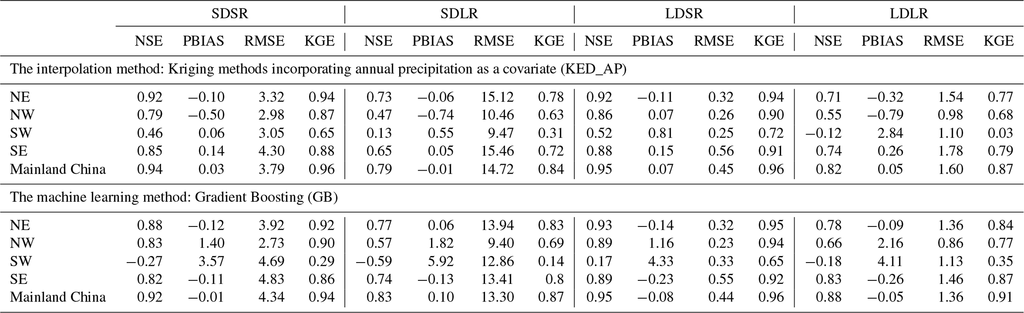
The machine learning method, GB, demonstrates notable adaptability across most regions and is often comparable to or better than interpolation methods, particularly for longer durations and return periods. As shown in Table 4, in the NE region, GB achieves a KGE of 0.92 for SDSR, closely matching KED_AP's performance of 0.94. For LDSR, GB's KGE reaches 0.95, slightly exceeding that of KED_AP. In the SE region, although GB slightly underperforms KED_AP for shorter durations and return periods (e.g., KGE of 0.86 for SDSR compared to 0.88 for KED_AP), its relative performance improves as duration and return period increase. For example, for LDLR, GB achieves a KGE of 0.87, surpassing KED_AP's KGE of 0.79. Similarly, in the NW region, GB's performance for LDLR reaches a KGE of 0.77, exceeding KED_AP's KGE of 0.68. However, in the SW region, GB's performance is considerably lower than that in other regions across all four IDF cases, with the highest KGE reaching only 0.65. This underperformance is likely attributable to the pronounced terrain undulation and sparse station distribution in the SW region, where the complex precipitation patterns are challenging for a nationally trained GB model to capture accurately. Additionally, the representativeness errors in the gridded precipitation data may further hinder the accuracy of the machine learning method in this region. Overall, the results demonstrate that GB exhibits notable adaptability across most regions, with its predictive accuracy relative to interpolation methods improving as duration and return period increase, thereby demonstrating the robustness of this trend at the national level.

3.4 The regionalized IDF curves in Mainland China

Figure 6 shows the spatial distribution of four cases predicted by KED_AP and GB. Both methods reveal a spatial pattern with a decreasing trend from the southeastern coastal areas to the northwestern interior, with overall similar distributions. This distribution is consistent across different durations and return periods, highlighting the influence of China's varied climatic and topographic conditions. In the SE region, which is characterized by humid subtropical and monsoon climates, higher extreme rainfall intensities are evident. This region experiences the most intense rainfall due to its proximity to oceanic moisture sources, frequent passage of typhoons, and summer monsoon systems. The reduction in extreme rainfall intensity moving inland reflects the weakening of moisture-laden winds as they traverse the country and encounter various geographical barriers, such as the Tibetan Plateau. This trend aligns with another study on design rainstorms with a 2-year return period and a 20 min duration in China, which shows significantly higher rainstorm amounts in the east compared to the west, and in the south compared to the north (Shao and Liu, 2018). However, notable local differences between both methods can be observed. The interpolated rainfall intensity appears smoother and more uniform. In contrast, the machine learning method exhibits weaker local autocorrelation, resulting in more abrupt spatial changes (Fig. 6). Interpolation relies on distant stations, leading to values that are closer to those observed at existing stations, producing a more homogeneous spatial distribution. The machine learning method, however, is more influenced by local geographical conditions, resulting in greater spatial heterogeneity and highlighting the diversity of the terrain and climate.

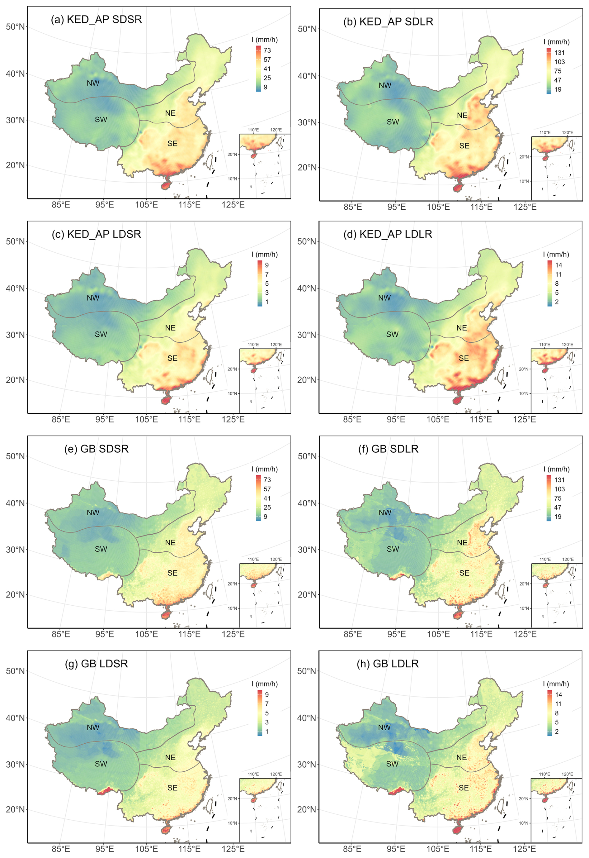
Figure 6 Spatial distribution of predicted rainfall intensity (mm h⁻¹) from KED_AP (the best interpolation method, a–d) and GB (the best machine learning method, e–h).

Notably, the machine learning method predicts local peaks in the southeastern edge of the SW region, which are not captured by the interpolation results (Fig. 6). This discrepancy was also found in comparisons of rainfall erosivity (i.e., the potential for water erosion caused by rainfall) estimated with Global Climate Models (GCM) generated rainfall and gauge-observed hourly rainfall (Wang et al., 2023), which likely arises from the influence of orographic rainfall on the windward slopes, leading to more extreme precipitation in this area. The machine learning method can detect this feature from the grid data. In contrast, the interpolation method, constrained by the sparse distribution of rain gauges, extrapolates the rainfall intensity from surrounding areas with less rainfall, thereby missing this localized phenomenon. This underscores the advantage of machine learning methods based on gridded precipitation data in regions where station data is sparse or unavailable.

4 Discussion

Effectiveness of different regionalization methods was comprehensively evaluated in this study for estimating regionalized IDF curves across mainland China. Specifically, the IDF curves were regionalized using five traditional interpolation methods – Inverse Distance Weighted (IDW), Ordinary Kriging (OK), Kriging with External Drift using annual average precipitation (KED_AP), Kriging with External Drift using elevation (KED_DEM), and Kriging with External Drift using both elevation and annual average precipitation (KED_DEM+AP) – along with five different machine learning methods: Random Forest (RF), Gradient Boosting (GB), Extremely Randomized Trees (ET), Multilayer Perceptron (MLP), and Linear Regression (LR). To evaluate the accuracy, each regionalization method was compared against site-specific IDF curves used as benchmarks. In addition, this study attempted to test whether any of the methods combined daily precipitation data could be satisfactorily used to regionalize and extrapolate IDF curves for storm durations much shorter than 24 h.

The comparison of interpolation and machine learning methods for IDF curves across mainland China reveals several notable patterns and insights. Our analysis demonstrates that both methods can effectively estimate extreme rainfall intensities, with the best-performing methods from each category – KED_AP for interpolation and GB for machine learning – achieving comparable accuracy levels. Furthermore, the relationship between prediction accuracy and IDF cases exhibits clear patterns: both methods show decreased performance with shorter durations and larger return periods. This pattern aligns with the inherent challenges in predicting more extreme and temporally concentrated rainfall events. KED_AP outperforms other interpolation methods, such as OK and KED_DEM, likely because the annual average precipitation is a more effective covariate for capturing the spatial patterns of extreme rainfall across diverse terrains compared to other covariates considered in this study. This advantage may stem from its strong correlation with extreme precipitation, whereas elevation, despite some correlation with extreme precipitation in regions of complex topography, appears less effective in flatter regions where its influence on extreme precipitation diminishes (Zou et al., 2021). As for machine learning methods, ensemble learning techniques, particularly GB, have demonstrated stable and excellent performance. To assess the interpretability of the GB model, a feature importance analysis using Shapley Additive Explanations (Lundberg and Lee, 2017) was conducted (Fig. S4). This analysis reveals that the model's predictive power is primarily driven by features derived from the gridded precipitation data characterizing daily extremes, specifically the gridded daily precipitation of varying return periods and the average annual maximum daily precipitation. This is likely because the model effectively learns the strong correlation between extreme precipitation events at sub-daily scales and corresponding daily gridded precipitation extremes, capturing this shared pattern across numerous samples through its non-linear capabilities. Furthermore, geographic variables like latitude, longitude, and elevation consistently rank as important secondary features. These variables establish the background precipitation gradient controlled by climatic and topographic factors across mainland China. This spatial baseline, together with daily extreme precipitation features, enables the model to produce spatially heterogeneous IDF estimations.

The national-level analysis, however, raises an important question about the spatial consistency of these findings. While both methods demonstrate robust overall performance, their effectiveness may vary across the diverse geographical and climatic regions in mainland China. This consideration is particularly relevant given the country's complex topography and rainfall patterns. Therefore, it is essential to examine how these methods perform across different regions. The analysis in Sect. 3.3 reveals that both methods achieve acceptable accuracy in the NE, SE, and NW regions, while in the SW region, both methods show reduced performance, with the machine learning method exhibiting lower accuracy than the interpolation method (Table 4). Figure 7 further illustrates IDF curves from representative stations in each of the four regions, indicating that both the interpolation and machine learning methods produce IDF curves with low uncertainty and high consistency with observed curves. This further corroborates the reliability of both methods. The performance discrepancy between the interpolation and machine learning methods in the SW region is likely because, despite the overall lower station density and complex terrain in the SW region, the training and validation stations are relatively concentrated, thereby reducing the limitations imposed by station density on interpolation accuracy (Fig. 1). This suggests that the interpolation method may exhibit reduced predictive accuracy in the western areas of the SW region, where validation stations are sparsely distributed, although this conclusion cannot be confirmed due to the absence of observational data for verification. In comparison, the accuracy of the machine learning method is more constrained by the availability of local samples. The machine learning model, trained on national station data, cannot accurately capture the unique rainfall patterns in the SW region due to the limited number of local training stations there. In addition, the representativeness errors inherent in gridded precipitation data could further impair the machine learning method's predictive accuracy in this region.

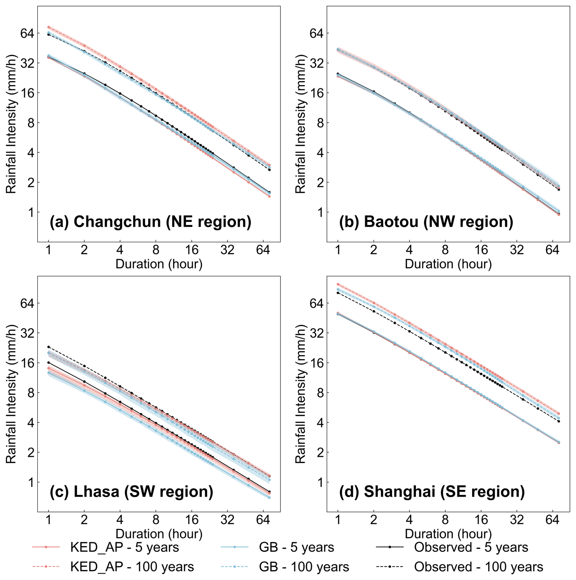
Figure 7 IDF curves using KED_AP (interpolation method), GB (machine learning method), and observed data for (a) Changchun in the NE region, (b) Baotou in the NW region, (c) Lhasa in the SW region, and (d) Shanghai in the SE region, with return periods of 5 and 100 years. For all stations in the mainland China except the four shown, 80 % were randomly selected as training samples for both interpolation and machine learning methods, with this process repeated 500 times using Monte Carlo sampling to predict the IDF curves for these four stations. Black lines represent the observed IDF curves, red lines represent the mean of the 500 samples for the interpolation method, and blue lines represent the mean for the machine learning method, with solid lines indicating the 5-year return period and dashed lines indicating the 100-year return period. Shaded areas correspond to the 2.5th and 97.5th percentiles of the 500 samples.

A particularly interesting finding is the gradual shift with duration and return period in relative performance between the two methods evaluated. As duration and return period increase, the accuracy of machine learning in most regions gradually improves, eventually approaching or even surpassing the interpolation, consistent with the national evaluation (Table 4 and Fig. 3). The enhanced relative performance of machine learning methods for longer durations may be attributed to the disparity in the temporal resolution of the independent variables (Table 1). Specifically, the interpolation utilizes station rainfall data with higher temporal resolution (hourly), whereas the machine learning relies on daily gridded precipitation data. Consequently, the accuracy of the interpolation remains relatively unaffected by shorter durations, whereas machine learning exhibits reduced predictive capability for short-duration rainfall events but demonstrates its inherent predictive advantages for long-duration rainfall. This suggests that utilizing gridded precipitation data with higher temporal resolution as independent variables would likely lead to improved accuracy in regionalized IDF curves based on machine learning. Furthermore, the enhanced relative performance of machine learning methods for larger return periods may stem from their ability to better handle extreme rainfall events, where the assumptions of spatial autocorrelation required by interpolation methods become less tenable. Machine learning models make better use of local precipitation and topographical features, allowing them to capture the complex non-linear relationships between these features and extreme rainfall more effectively than interpolation methods.

Further practical differences between interpolation and machine learning methods were identified that generally apply in various contexts. The machine learning approach is useful in applications where a trained model may be used to make predictions for areas without observations. This means that machine learning is particularly useful for forecasting of future prediction surfaces, while in contrast, forecasting is not possible with interpolation techniques that always require point observations. By comparison, interpolation techniques may be preferable for producing prediction surfaces for historical time frames where observations are available. The geospatial approach used by most interpolation methods considers data in the surrounding neighborhood of the point for prediction. Consequently, interpolation methods may be expected to result in smoother surfaces with a higher degree of spatial autocorrelation compared to the test machine learning methods that only consider information where prediction is attempted. Therefore, the choice of prediction method may depend on the context of the application and the available data.

Several limitations regarding data availability and methodological assumptions should be noted. While our study found that the accuracies of machine learning and interpolation are comparable, this conclusion may change as more validation stations are included. For instance, given that interpolation accuracy is constrained by station density, large areas in the NW and SW regions both lack stations and are distant from existing stations (Fig. 1), likely resulting in severely affected interpolation accuracy in these areas. Similarly, since the accuracy of machine learning is constrained by the availability of non-local samples, and the gridded precipitation datasets in these regions may have been significantly underestimated (Miao et al., 2024), the results derived from machine learning based on these datasets may also be severely affected. Due to the lack of stations for verification, these remain unconfirmed and will need to be validated with installation of additional stations in the future. It is also important to note that, although regionalized IDF were generated for the NW and SW regions in this study, their use should be approached with caution due to the lack of station-based verification. Users are strongly advised to consider the higher uncertainty associated with predictions in these areas and validate results against local observations if available. For the SW region, an alternative high-resolution IDF dataset (1$/$30°) trained with local samples offers a valuable supplement to our work (Ren et al., 2025). While our study focuses on the robustness and general applicability of regionalization methods at a near-national scale across diverse climates and topographies, their study concentrates on achieving high-resolution regionalization within one of the most complex regions in mainland China. Another limitation worth noting is that our study employed stationary IDF curves derived from historical observations, assuming temporal invariance in the extreme precipitation distribution. With climate change both the frequency and intensity of extreme precipitation events are expected to increase, thereby affecting the distributional parameters. Future studies should investigate how these regionalization methods perform under non-stationary conditions. Furthermore, limitations inherent in the observational records must be acknowledged, specifically the uncertainty associated with extrapolating 10–70 years of records to 1000-year return periods, and the exclusion of sub-hourly events due to the minimum input duration of one hour.

Finally, this study not only highlights the promise of machine learning but also points to opportunities for further refinement. The potential for improving the accuracy of interpolation methods in this study area is limited, due to the lack of higher station density and finer temporal resolution observations. Conversely, machine learning methods have substantial room for improvement through enhanced temporal and spatial resolution of gridded precipitation data, improved data quality, incorporation of additional meteorological variables such as temperature, relative humidity, and atmospheric circulation patterns, as well as the development of more advanced machine learning techniques and exploration of more comprehensive hyperparameter combinations not considered in this study. Such advancements could significantly improve the predictive capabilities beyond the results demonstrated in this study.

5 Conclusions

This study explored optimal methods for regionalizing Intensity-Duration-Frequency (IDF) curves across mainland China, utilizing long-term hourly precipitation data from 2363 observation stations across mainland China, as well as daily gridded precipitation data from the CHM_PRE. To achieve this objective, we evaluated and compared the performance of five traditional interpolation methods (site-observation-based) and five emerging machine learning methods (gridded-precipitation-based). Four representative rainfall intensities were selected as examples: 1 h, 5-year (SDSR), 1 h, 100-year (SDLR), 24 h, 5-year (LDSR), and 24 h, 100-year (LDLR). The following key findings were obtained:

Among all interpolation methods evaluated in this study, Kriging methods incorporating annual precipitation as a covariate (KED_AP) significantly improved prediction accuracy compared with the Ordinary Kriging (OK), whereas including elevation as a covariate did not improve the accuracy. Among all machine learning methods evaluated in this study, Gradient Boosting (GB) demonstrated the best and most robust performance.

For the best-performing interpolation and machine learning methods across the four rainfall intensities selected, both methods demonstrated comparable and robust performance across various cases, whether for short or long durations and return periods. Specifically, the KED_AP method achieved a KGE of over 0.96 for SDSR and LDSR, and over 0.84 for SDLR and LDLR. Similarly, the GB method achieved a KGE of over 0.94 for SDSR and LDSR, and over 0.87 for SDLR and LDLR. Machine learning methods tend to perform better as the duration and return period increase. Besides, shorter durations and larger return periods were associated with increased prediction difficulty and reduced accuracy for both methods, as evidenced by the KGE values for LDSR (KED_AP = 0.96; GB = 0.96) and SDLR (KED_AP = 0.84; GB = 0.87).

IDF curves typically require precipitation data with sub-daily temporal resolution (e.g., hourly) when using traditional interpolation methods. In contrast, machine learning methods, utilizing only daily precipitation data and not previously applied to IDF curves regionalization in mainland China, demonstrated comparable accuracy to traditional methods and even outperformed them for long durations and large return periods. Additionally, machine learning offers distinct advantages, such as only requiring coarser temporal resolution precipitation data, being less dependent on station setup conditions, and possessing strong adaptability for future updates. These advantages suggest that machine learning has the potential to replace interpolation methods to produce future IDF curves.

With the optimal regionalization method for each specific duration and return period, the study ultimately produced a regionalized IDF curves product for mainland China with a spatial resolution of 0.1°×0.1°. The durations considered ranged from 1 to 24 h, along with 36, 48, and 72 h, and the return periods included 2, 5, 10, 20, 50, 100, 200, 500, and 1000 years. Although with lower accuracy, another IDF curves product for mainland China with a spatial resolution of 0.5°×0.5° based on CGDPP, is also provided as an alternative. To resolve potential crossing phenomena within the generated curves, a bivariate isotonic regression was applied as post-processing, ensuring physical consistency with negligible impact on accuracy (Dykstra, 1983). We also provided accuracy metrics and the name of the optimal regionalization methods for each IDF case (Tables S31, S36, S41–S48). Taking the city of Beijing (approximately 16 000 km²) as an example, the existing hourly gauges provide about 20 station-level IDF curves. Our 0.1° dataset increases this to about 170 available IDF curves, while the 0.5° dataset provides about 8 curves. The 0.1° dataset is recommended for local-scale applications requiring high spatial detail, for urban drainage design and small catchment flood modeling for example, while the 0.5° dataset is appropriate for regional-scale hydrologic modeling where computational efficiency and areal-average representation are prioritized.

In summary, this study advances regionalization of IDF curves with several distinct contributions that enhance both methodological understanding and practical application. First, through a systematic comparison of traditional interpolation and emerging machine learning methods, this research highlights the relative strengths of each method, enabling the identification of optimal regionalization strategies tailored to specific duration and return period combinations. Second, the study demonstrates that machine learning methods, using readily available gridded daily precipitation data, can estimate sub-daily IDF curves with accuracy comparable to traditional interpolation methods using hourly data. This finding is particularly significant for regions where high-temporal-resolution data are scarce, as it expands the potential for effective IDF regionalization in data-limited environments. Third, by generating a regionalized dataset on IDF curves for mainland China where such datasets were previously scarce, this study has generated a valuable resource for flood risk assessment and infrastructure planning, while providing a valuable methodological framework for similar studies in other regions.

Appendix A: List of important acronyms and their definitions

Acronym	Definition
ET	Extremely Randomized Trees
GB	Gradient Boosting
GEV	Generalized Extreme Value
IDF	Intensity-Duration-Frequency
IDW	Inverse Distance Weighting
KED	Kriging with External Drift
KED_AP	Kriging with External Drift using Mean Annual Precipitation
KED_DEM	Kriging with External Drift using Elevation
KGE	Kling-Gupta Efficiency
LDLR	Long Duration-Large Return Period
LDSR	Long Duration-Small Return Period
LR	Linear Regression
ML	Machine Learning
MLP	Multilayer Perceptron
NE	Northeastern Monsoon Region
NSE	Nash-Sutcliffe Efficiency
NW	Northwestern Arid Region
OK	Ordinary Kriging
PBIAS	Percent Bias
RF	Random Forest
RMSE	Root Mean Square Error
SDLR	Short Duration-Large Return Period
SDSR	Short Duration-Small Return Period
SE	Southeastern Monsoon Region
SW	Southwestern Tibetan Plateau Region