Reconstructed soil moisture droughts in Belgium reveal 2011–2020 was the driest decade since 1970

In recent years, Belgium has experienced a sequence of intense droughts with wide-ranging impacts across multiple sectors. Determining whether these events are unprecedented or within natural variability requires indicators that properly diagnose drought. Root-zone soil moisture is a suitable indicator because it integrates meteorological forcings with land-surface processes. In Belgium, however, operational monitoring relies mainly on precipitation-based indices and lacks long-term in situ soil-moisture observations, leaving uncertainty about whether these indices capture the persistence of root-zone drought. To address this gap, we reconstructed daily root-zone soil-moisture dynamics over Belgium from 1970 to 2020 using the mesoscale Hydrologic Model (mHM), placing recent droughts in historical context and evaluating the adequacy of precipitation-based indicators for representing drought conditions. Our analysis shows that droughts in 2011–2020 were unprecedented in both duration and severity over the past five decades. Between 2011 and 2020, the country experienced a cumulative three years (non-consecutive) of drought exposure, representing 30 % of the decade. This more than doubles the cumulative duration in each decade from 1981 to 2010 and is about 1.5 times that of 1971 to 1980.

We further find that the Standardized Precipitation–Evapotranspiration Index (SPEI), currently used operationally as a proxy for agricultural droughts in Belgium, underestimates the persistence of root-zone droughts because it does not explicitly account for land-surface memory. Thus, by including soil moisture monitoring in drought assessment, residual stresses on agriculture and subsurface water, which can persist long after meteorological conditions have normalized, can still be detected. This gives decision-makers a more realistic understanding of droughts and how to respond proportionately.

1 Introduction

Belgium has experienced a succession of severe droughts in recent years, with major impacts on agriculture, water resources, and inland navigation, resulting in economic losses amounting to hundreds of millions of euros (Tröltzsch et al., 2016; De Ridder et al., 2020).

The cross-sectoral impacts of the successive droughts of 2016–2017 and 2018–2019 were particularly significant. To demonstrate, in the Flemish Region¹, the 2018–2019 drought caused widespread crop losses, prompting farmers to submit compensation claims of about EUR 150 million to the Flemish Disaster Fund (De Ridder et al., 2020). Low water levels arising from the drought also disrupted inland navigation and caused an estimated EUR 283 million in economic damage (De Vlaamse Waterweg nv, 2022). In the Walloon Region, the drought similarly affected agriculture and water availability, and the period from June to August 2018 was officially recognized as an agricultural disaster, with about EUR 31.5 million allocated in compensation to affected farmers (Le sillon Belge, 2019; Thibaut et al., 2023). Similar impacts were experienced during another drought in 2022, where at the peak of the drought in July that year, the country received only 5 mm of precipitation, the lowest monthly total for July in 137 years (since 1885). Groundwater levels in Belgium consequently fell to their lowest levels since at least 2000 (DOV, 2025; Piézométrie du Service Public de Wallonie, 2025), and in many locations they did not fully recover during the following winter (VMM, 2023).

Although the impacts of these recent droughts are well documented, their significance in a longer climatological context remains unclear. In particular, it is not yet known whether the recent clustering of severe droughts represents a departure from earlier decades or falls within the range of natural climate variability in Belgium. Addressing this question requires a reconstruction of drought occurrence over a sufficiently long period, based on indicators that adequately capture the propagation and persistence of drought within the hydrological system.

Drought is characterized in several ways; in this manuscript we focus on three commonly used forms. Meteorological drought describes a persistence of precipitation shortage, agricultural drought refers to a sustained deficit in soil moisture which causes plant water stress, while hydrological drought indicates shortages in surface and subsurface water supplies (Mishra and Singh, 2010). In Belgium there is an extensive network of precipitation, river discharge and groundwater monitoring stations which provide the basis for monitoring hydrological and meteorological droughts. These data underlie the drought indices found in dedicated platforms for tracking and communicating the evolution of droughts across the country (e.g. https://www.meteo.be/en/weather/forecasts/drought, last access: 10 September 2025; https://vmm.vlaanderen.be/water/droogte, last access: 10 September 2025). Due to the lack of long-term observations of soil moisture in the country, the extent of agricultural droughts is presently evaluated with the Standardized Precipitation Evaporation Index (SPEI) (Vicente-Serrano et al., 2010) which expresses anomalies in the climatic water balance, that is, precipitation minus potential evapotranspiration. The nationwide drought conditions are reported through https://www.meteo.be/en/weather/forecasts/drought (last access: 10 September 2025).

Although useful, precipitation- and temperature-based drought indices are constrained by their limited ability to fully represent agricultural drought conditions. Firstly, these indices do not explicitly account for the vertical distribution of water within the root zone that supports plant growth, nor do they reflect the complex interactions between soil moisture and vegetation across different stages of plant development and are thus inadequate to represent extreme water shortage that would lead to biomass and crop yield reduction (Sheffield et al., 2004; Mishra and Singh, 2010; Samaniego et al., 2013). While soil moisture may exhibit a direct link to precipitation at monthly timescales, soil moisture responses can be nonlinear at shorter timescales, particularly during dry conditions. Soil moisture also has a memory effect that can lag precipitation anomalies by days to months and in turn prolong the persistence and severity of drought (Bonan and Stillwell-Soller, 1998; Nicholson, 2000; Wu et al., 2002; Seneviratne et al., 2006). Accordingly, developing indices based on soil moisture offers a more reliable indicator of agricultural drought, as soil moisture integrates the effects of antecedent precipitation, plant water uptake through transpiration, and the increasing persistence of soil wetness with soil depth (Wu et al., 2002; Sheffield et al., 2004).

The goal of this study is therefore to produce a retrospective high-resolution reconstruction of root-zone soil moisture and use it to provide a first assessment of soil-moisture droughts in Belgium over the five decades from 1970 to 2020. We aim to characterize major droughts that have occurred over this period by clustering soil moisture anomalies using thresholds that capture the spatiotemporal characteristics of identified events and rank them based on their magnitude, spatial extent and duration, and evaluate how drought patterns in the country have evolved over the five decades. To evaluate the correspondence between SPEI and soil moisture-based anomalies to represent agricultural droughts, we compare SPEI at different accumulation periods to a soil moisture index (SMI) (Samaniego et al., 2018) during selected major drought events.

2 Methodology

2.1 Study domain

Belgium is located in Western Europe covering an area of 30 528 km², varying in topography from sea level along the North Sea coast to 700 m in the Ardennes-Eifel massif in the south eastern parts (Fig. 1) (Meersmans et al., 2016; Sousa-Silva et al., 2016). The country experiences a warm temperate maritime climate (Köppen-Geiger Cfb) strongly modulated by the warming effect of the North Atlantic Drift (Erpicum et al., 2018; Beck et al., 2023). Data from the Royal Meteorological Institute of Belgium (RMI) shows that mean annual temperature ranges between 13 and 17 °C, varying spatially with elevation and distance inland. Winters are generally mild, with December–January lows dipping under 5 °C but rarely below freezing conditions for long periods. Winters are colder in the Ardennes region due to a weaker maritime influence and higher elevation. Summers are moderately warm with July highs peaking around 18 °C although extremes above 30 °C have occurred in recent years. The country receives an annual average precipitation of about 800 mm which varies between 700 mm in the western low lying regions, up to 1400 mm in the Ardennes where precipitation is enhanced by orographic effects (Erpicum et al., 2018). Temporally, rainfall is fairly evenly distributed throughout the year (Fig. 1), with seasonal patterns dominated by summer convective storms and winter frontal systems (Brisson et al., 2011; Goudenhoofdt and Delobbe, 2013; Journée et al., 2015).

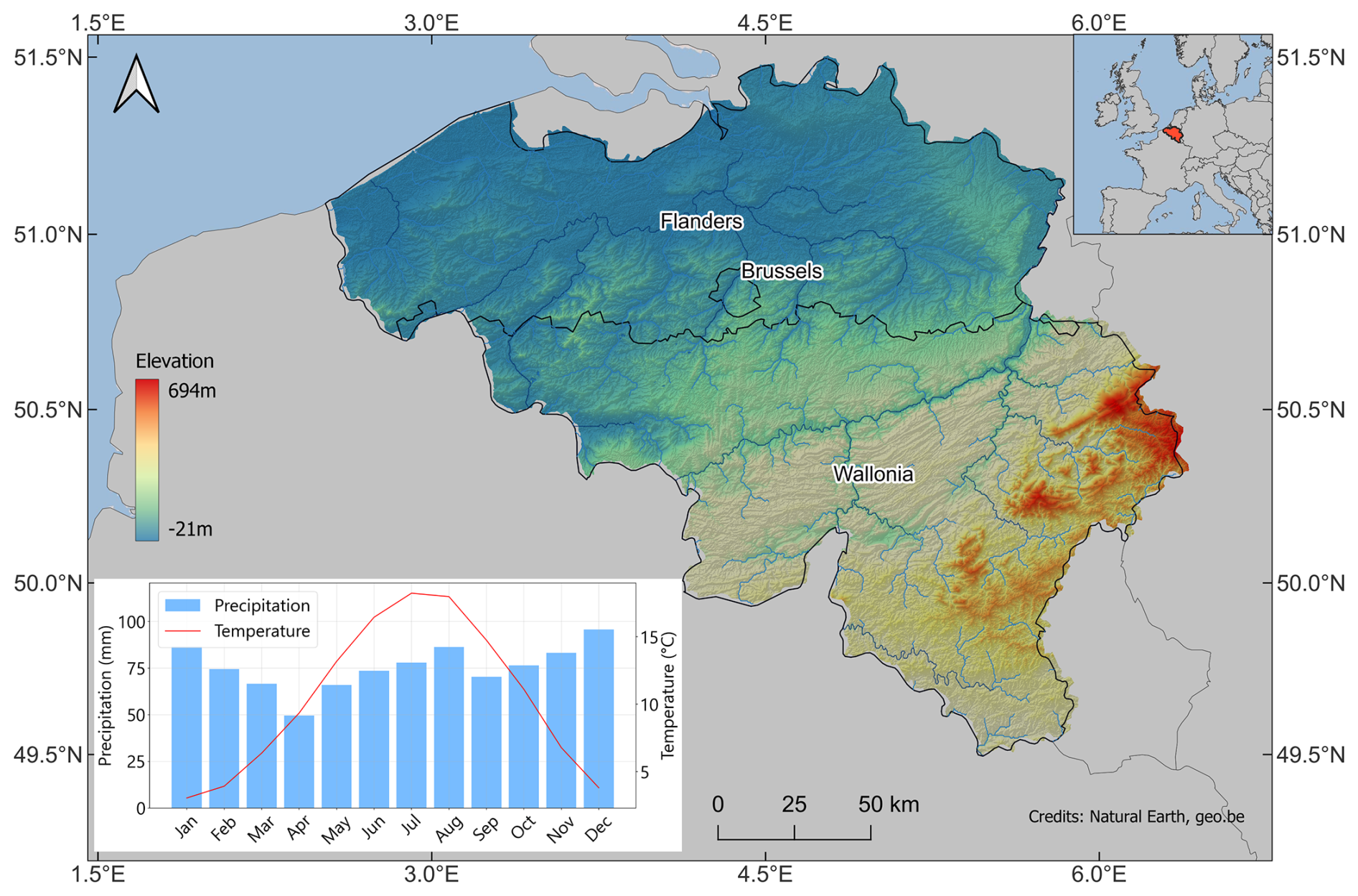
Figure 1 Topographic map of Belgium. The Ardennes region is distinguishable by its high elevation in the south-east. Monthly mean precipitation and temperature in the inset plot are derived from data provided by The Royal Meteorological Institute of Belgium for the climatological period 1994–2023.

Land cover in the country is predominantly agricultural (44 %), dominated by croplands and animal husbandry. Cultivated areas dominate the central loamy belt and the northwest of the country while the coastal polders typified by heavy soils, are more suited for animal-based farming (Beckers et al., 2018, 2020; Statbel, 2025a). Forests cover about 23 % of the territory (just over 700 000 ha) with 79.8 % in the Walloon region, 19.9 % in Flanders and 0.3 % in the Brussels-Capital (Sousa-Silva et al., 2016; Royal Forestry Society of Belgium, 2025). Most of the lowland forests are dominated by broad-leaved tree species with clusters of coniferous forest plantations in the northeast. In the Ardennes, forests form a mixed broadleaved–coniferous complex in the foothills, gradually transitioning to conifer-dominated stands at higher elevations (Royal Forestry Society of Belgium, 2025; Statbel, 2025a). Built-up and urbanized areas account for about 20 % of the land with most cities dating back to the Middle Ages. The average population density of the country is 385 inhabitants per km² (Beckers et al., 2020; Statbel, 2025b).

2.2 The mesoscale Hydrologic Model

In our study, we used the mesoscale Hydrologic Model (mHM; Samaniego et al., 2010; Kumar et al., 2013) (version v-5.13.2-dev0) to simulate domain-wide root-zone (0–2 m) soil moisture conditions and streamflow, which we used as an additional hydrologic constraint for validating basin-scale hydrology at major outlets.

mHM is a spatially distributed hydrological model based on numerical representations of dominant hydrological processes. The model is driven by hourly to daily meteorological forcings, which include precipitation, air temperature (henceforth simply temperature), and potential evapotranspiration, and accounts for major hydrological processes like snowmelt and accumulation, canopy storage, evapotranspiration, surface runoff and flood routing, three-layer soil moisture content, and subsurface storage. To represent spatial variability of inputs and state variables, the model uses three different spatial resolutions, namely (in order of fine to coarse resolution) Level-0 (L₀: small-scale morphology) to represent the main terrain features, geological features, land cover, and soil properties; Level-1 (L₁: mesoscale hydrology) to represent the dominant hydrological processes; and Level-2 (L₂: large-scale meteorology) to describe the variability of meteorological forcings. The model harmonizes the data internally using the multiscale parameter regionalization (MPR; Samaniego et al., 2010). MPR links model parameters at L₁ to their corresponding ones at L₀ using non-linear transfer functions that couple catchment characteristics with global (calibration) parameters to regionalize model hydrologic parameters at L₀ and link them to their corresponding values at L₁ using upscaling operators such as arithmetic mean, geometric mean, and harmonic mean (MPR; Livneh et al., 2015). With this technique, mHM achieves quasi scale-invariant parameters that enable the model to preserve the spatial variability of state variables and conserve mass balance (Samaniego et al., 2010, 2011; Kumar et al., 2013; Samaniego et al., 2013). mHM has been successfully used in multiple studies at scales ranging from river basins (Zink et al., 2017; Dembélé et al., 2020; Demirel et al., 2024; Banjara et al., 2025), country level (Samaniego et al., 2013; Rakovec et al., 2019; Boeing et al., 2022) up to continental-scale (Samaniego et al., 2018; Moravec et al., 2019; Kumar et al., 2025) and global studies (Řehoř et al., 2025; Shrestha et al., 2025).

2.2.1 Input data

Our simulation is driven by daily fields of precipitation and temperature from the ENSEMBLES gridded dataset (E-OBS) version 30.0e (Cornes et al., 2018), which covers the entire modelling domain. E-OBS is a daily land-only gridded observational dataset over Europe which blends station network time series from the European National Meteorological and Hydrological Services or other sources and is provided with spatial resolutions of 0.1° and 0.25°. Our setup uses the 0.1° resolution product (access URL: https://cds.climate.copernicus.eu/datasets/insitu-gridded-observations-europe?tab=download, last access: 7 March 2025). Since E-OBS does not provide potential evapotranspiration data, we generated this from the E-OBS minimum and maximum temperature using the method of Hargreaves and Samani (1985).

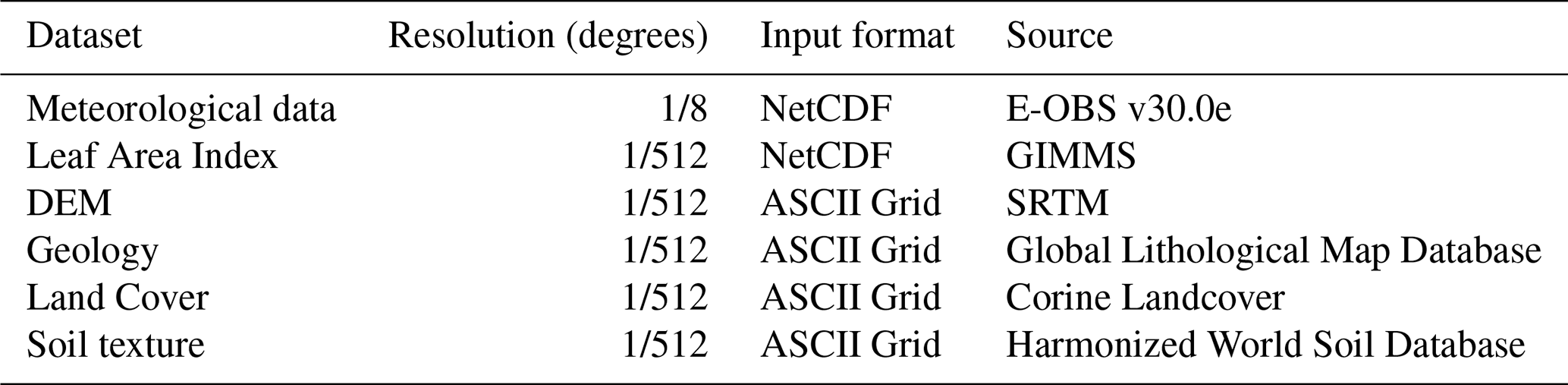
The morphological datasets for the model originate from different sources, namely, LAI maps from Global Inventory Modeling and Mapping Studies (GIMMS) (Cao et al., 2023), DEM from the Shuttle Radar Topography Mission (Farr et al., 2007), land use data from Corine Land Cover (https://land.copernicus.eu/en/products/corine-land-cover, last access: 7 March 2025), soil texture and bulk density data from the Harmonized World Soil Database (FAO and IIASA, 2023), and geology datasets from the Global Lithological Map Database (Hartmann and Moosdorf, 2012), accessed from the URL: https://www.geo.uni-hamburg.de/geologie/forschung/aquatische-geochemie/glim.html (last access: February 2025). To ensure the spatial consistency required by mHM, we prepared all L₀ datasets at 0.001953125° ($\mathrm{1}/\mathrm{512}\mathit{°}$), bilinearly coarsened the L₂ meteorological data to 0.125° ($\mathrm{1}/\mathrm{8}\mathit{°}$), and set the resolution of L₁ to 0.03125° ($\mathrm{1}/\mathrm{32}\mathit{°}$), these are summarized in Table 1. We then ran the model from 1965 to 2020, including a warm-up period of 5 years at the beginning.

Table 1 Data sources and spatial resolutions used in the mHM setup.

Long-term in situ soil moisture data to validate the soil moisture output of mHM is not available within Belgium, so we expanded the model domain to cover parts of France, Germany and the Netherlands, where soil moisture observations are available from the International Soil Moisture Network (ISMN) (Dorigo et al., 2021). From the ISMN, we used data from the following networks: COSMOS (Zreda et al., 2008), GROW (Xaver et al., 2020), TERENO (Bogena et al., 2018), BFG₋Nw and ORACLE, all shown in Fig. 2.

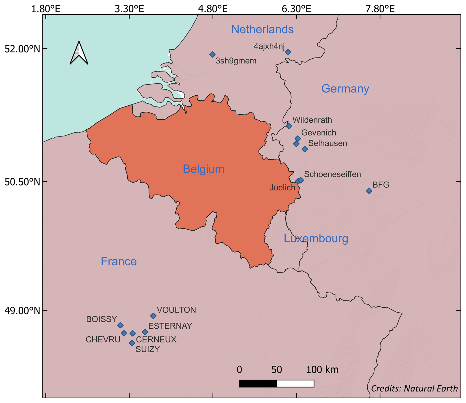
Figure 2 Locations of ISMN stations (blue diamonds) used to validate mHM soil moisture.

2.2.2 mHM Soil Moisture simulation

mHM calculates water infiltration between soil layers using an exponential function that accounts for the nonlinearity of soil water retention (Samaniego et al., 2010; Livneh et al., 2015). Briefly, for a given soil layer, k, on pervious areas, the infiltration I_k into the layer is determined by the equation:

$$\begin{array}{}\text{(1)}& I_k=I_{k-\mathrm{1}}\cdot {\left({\displaystyle \frac{{\mathit{\theta }}_k}{{\mathit{\theta }}_{\mathrm{sat},k}}}\right)}^{{\mathit{\beta }}_k}\end{array}$$

I_k−1 represents the infiltration from the previous layer k−1, θ_k is the soil moisture of layer k, θ_sat,k is the saturation moisture content for the layer, and β_k is an exponential parameter that adjusts for the non-linear nature of soil moisture retention. Once infiltration is calculated, the model updates soil moisture θ_t by adding the difference between the layer infiltration I_t and actual evapotranspiration (ET_t) for the time step as;

$$\begin{array}{}\text{(2)}& {\mathit{\theta }}_t={\mathit{\theta }}_{t-\mathrm{1}}+I_t-{\mathrm{ET}}_t\end{array}$$

Actual evapotranspiration is calculated by reducing the potential evapotranspiration (PET) based on a soil moisture stress factor, f_SM, which varies depending on the soil moisture content.

$$\begin{array}{}\text{(3)}& \mathrm{ET}=f_{\mathrm{roots}}\cdot f_{\mathrm{SM}}\cdot \mathrm{PET}\end{array}$$

f_roots is the fraction of roots in the soil horizon and f_SM is calculated using either the Feddes equation (Feddes, 1982):

$$\begin{array}{}\text{(4)}& f_{\mathrm{SM}}={\displaystyle \frac{\mathit{\theta }-{\mathit{\theta }}_{\mathrm{pwp}}}{{\mathit{\theta }}_{\mathrm{fc}}-{\mathit{\theta }}_{\mathrm{pwp}}}}\end{array}$$

or the Jarvis equation (after Jarvis, 1989):

$$\begin{array}{}\text{(5)}& f_{\mathrm{SM}}={\displaystyle \frac{\mathrm{1}}{{\mathit{\theta }}_{\mathrm{stress}-\mathrm{index}-\mathrm{C}\mathrm{1}}}}\cdot {\displaystyle \frac{\mathit{\theta }-{\mathit{\theta }}_{\mathrm{pwp}}}{{\mathit{\theta }}_{\mathrm{sat}}-{\mathit{\theta }}_{\mathrm{pwp}}}}\end{array}$$

The model uses the MPR routine to compute the saturation moisture content, field capacity (θ_fc) and wilting point (θ_pwp).

2.2.3 Model evaluation

The accuracy and spatial representativeness of absolute soil moisture values are strongly source-dependent (in situ or modelled), so direct comparisons between different datasets can be misleading (Koster et al., 2009; Ford and Quiring, 2019). On one hand, simulated soil moisture is highly dependent on the quality of meteorological forcings and the physical parameterization of the model (Koster et al., 2009; Wang et al., 2011; Nicolai-Shaw et al., 2015). On the other hand, in situ measurements are highly localized to the sensor location and are affected by the technology used by the sensor and the sufficiency of the calibration techniques (Peng et al., 2025). From a drought analysis perspective, the real information value of soil moisture is not in its absolute values but rather in its temporal variability metrics, such as anomalies and seasonal variability of soil wetness (Koster et al., 2009). This information value is generally more consistent and transferable between different sources when soil moisture is suitably normalised to have the same range and variability (Dirmeyer et al., 2004; Wang et al., 2011). Koster et al. (2009) show that if soil moisture from different sources differs only in their mean and standard deviation, then standardizing each time series (as in Eq. 6) would generate nearly identical datasets of standard normal deviations (θ^′).

$$\begin{array}{}\text{(6)}& {\mathit{\theta }}^{\prime }={\displaystyle \frac{\mathit{\theta }-{\mathit{\theta }}_{\mathrm{m}}}{{\mathit{\sigma }}_{\mathrm{m}}}}\end{array}$$

where θ is the soil moisture at a given point and time of year, θ_m and σ_m are the mean and standard deviation of soil moisture, respectively, for the same point and time of year.

In our evaluation of the mHM soil moisture, we used this approach to analyze the level of temporal agreement between the standard normal deviations of mHM and in situ soil moisture from the corresponding depths at the selected ISMN stations (Fig. 2).

For each in situ-modelled pair, we quantified the agreement in drought anomaly dynamics by calculating the Pearson correlation coefficient (r). To obtain an overall agreement across all sites, we first transformed the r values to the Fisher z-scale (z = arctanh(r)) to stabilize variance and avoid bias from the nonlinear r-scale. The z-values were then averaged to obtain $\stackrel{\mathrm{‾}}{z}$, and finally back-transformed to yield $\stackrel{\mathrm{‾}}{r}$ = tanh $\stackrel{\mathrm{‾}}{z}$.

Prior to the comparison, we performed a quality check on the in situ data to flag and exclude potentially erroneous measurements. We considered only errors due to systematic drift in measurements over time (jumps or drops) and spiky measurements that are not explained by random noise. Here we used the quality control algorithms on in situ soil moisture developed by Dorigo et al. (2013) considering only stations that have at least 10 years of observations.

Because soil moisture is also coupled with runoff through the terrestrial water budget, we added an independent check for model simulations against daily river-discharge observations from the major river basins in Belgium. For this, we used the inbuilt calibration feature of mHM and calibrated the model using data from river gauging stations all over the country, obtained from the Waterinfo database for Flanders (https://waterinfo.vlaanderen.be/Meetreeksen, last access: 16 May 2025) and the hydrometric network of discharge in Wallonia (https://hydrometrie.wallonie.be/home/observations/debit.html?, last access: 16 May 2025). In total we used 91 gauging stations during the calibration period (2000–2023) and 155 stations to validate the model from 1970 to 1999.

2.3 Characterizing soil moisture droughts

To characterize soil moisture droughts, we use a monthly soil moisture index (SMI), following Samaniego et al. (2013), considering the total soil water content of the root zone up to a depth of 0.5 m (we limit our analysis to this depth since groundwater in some regions is shallower than 0.5 m). For each month, grid cell soil moisture is expressed as a percentile relative to that month's historical soil moisture and scaled to a range between 0 and 1.

The computation of SMI in this study is based on the methodology of Samaniego et al. (2013), which proceeds as follows. Firstly, the monthly soil moisture averaged over the root-zone depth (0.5 m for this study) is extracted and used to compute a probability distribution function (PDF) f_t(x) for each grid cell as;

$$\begin{array}{}\text{(7)}& f_t\left(x\right)={\displaystyle \frac{\mathrm{1}}{nh}}\sum _{k=\mathrm{1}}^{n}K\left({\displaystyle \frac{x-x_k}{h}}\right)\end{array}$$

Where, x is the soil moisture value at which the PDF is evaluated x₁, …, x_k represent the simulated monthly soil moisture values for the month t over the simulation period. n is the number of calendar months within a given period (e.g., 50 for a 50-year period. Note that this conversion is done for each calendar month separately to account for inherent seasonality in SM simulations. K is a Gaussian kernel function and h is the bandwidth that controls the smoothness of the kernel (Eq. 8). The optimal value of h is computed using a cross-validation criterion.

$$\begin{array}{}\text{(8)}& K(x,x_k)={\displaystyle \frac{\mathrm{1}}{\sqrt{\mathrm{2}\mathit{\pi }{h}^{\mathrm{2}}}}}\exp \left({\displaystyle \frac{(x-x_k{)}^{\mathrm{2}}}{\mathrm{2}{h}^{\mathrm{2}}}}\right)\end{array}$$

The monthly grid cell SMI is then derived by integrating f_t(x) and the resulting SMI values are classified into percentiles. Drought-affected grid cells are identified using a threshold percentile τ, which is commonly set at 0.2 (e.g., Svoboda et al., 2002; Samaniego et al., 2013, 2018). This means that for a given month, a grid cell is experiencing drought if the soil moisture value falls below the 20th percentile of values for that month. According to Svoboda et al. (2002), this percentile represents the threshold at which the magnitude of drought begins to damage crops, cause water shortages and present high risks of fire. Next, adjacent cells where SMI ≤ τ (henceforth denoted as SMI_τ) at each timestep are consolidated to form drought clusters, which are defined by a minimum threshold area. Spatial clusters which share a minimum overlapping area at consecutive time steps are then joined to form multi-temporal clusters, each with a unique identity. For each cluster, the mean duration (months), areal extent from the onset to termination, and the total drought magnitude, which is the spatiotemporal integral of SMI_τ over the area affected, are computed. Following Samaniego et al. (2013), the magnitude of each event is computed as the space-time integral of the drought duration in months over the area under drought. This is represented mathematically as;

$$\begin{array}{}\text{(9)}& \mathrm{TDM}=\sum _{t=t_{\mathrm{0}}}^{t_{\mathrm{1}}}\underset{A_t}{\int }[\mathit{\tau }-{\mathrm{SMI}}_i(t){]}_{+}\end{array}$$

t₀ and t₁ represent the onset and termination month of a multi-temporal drought event, A_t is the area under drought at timestep t expressed as a percent of the total domain area, and + means the magnitude is computed only for the positive part of the function. To avoid detecting small, isolated and short-lived dry spells as droughts, we specified a minimum threshold area of 640 km² (about 2 % of total domain area), based on Samaniego et al. (2013) for an event to be considered as a drought and an overlap area of the same size for two drought events at successive time steps to be considered as a single multi-temporal drought cluster.

3 Results

3.1 Model Performance Evaluation

The daily standardized anomalies of mHM-simulated soil moisture evaluated against in situ observations from the ISMN are shown in Fig. 3. Of the 48 stations where in situ data was retrieved, 21 sites passed quality control checks and were retained for validating the model outputs. The resulting comparison showed that the two datasets are highly temporally correlated, with a mean Pearson $\stackrel{\mathrm{‾}}{r}$ = 0.86 (back-transformed averages from the Fisher z-scale), although the strength of the correlation varied with sensor depth and type. The correlation is lowest for the top 50 mm of the soil profile ($\stackrel{\mathrm{‾}}{r}$ = 0.81 for all networks) and increases to 0.86 for the profile depths greater than 150 mm.

Even for the selected in situ sites, some still exhibited spurious spikes outside of random noise (shown by the red scatter points in Fig. 3). We chose not to discard these points so as to preserve an adequate number of validation stations and to highlight the practical difficulty of obtaining perfectly reliable reference soil moisture data for validating model outputs. Despite such outliers, the model simulations and ISMN observation showed similar temporal variability in soil wetness and dryness. The difference mainly occurred in the top 50 mm layer during very dry episodes when mHM produced more extreme negative anomalies than most sensors (Fig. 3a–d). This explains why the correlation between the datasets is the lowest at this depth. We attribute this divergence partly to a flooring effect of capacitive sensors, which tend to plateau at very low volumetric water contents, whereas the model continues to resolve further drying. For deeper layers, the intensity and duration of dryness were more consistent between both datasets.

To evaluate how well the model simulates drought conditions, we investigated the drought-day detection skill (when the observed standardized anomaly fell below its 20th percentile) by counting hits (H; days when both model and observations indicate drought), misses (M; observed drought days not flagged by the model), false alarms (F; days flagged as drought by the model but not by the observations), and correct negatives (C; days when both indicate non-drought). (The methodology is described in more detail in Sect. S1 in the Supplement). From this analysis, we found that the model shows high skill in reproducing observed drought conditions, as it was able to detect 74 % of observed drought days from the 21 stations. The false alarm rate was also only 5 %, while the mean F₁ score (which summarizes the balance between misses and false alarms as $\mathrm{2}H/(\mathrm{2}H+F+M)$) was 75 %. We attribute the differences in detecting droughts to the scale mismatch between mHM soil moisture, which represents average conditions over a grid cell, and the highly localized nature of point in situ measurements. Nevertheless, these metrics indicate that the model can be applied to study droughts.

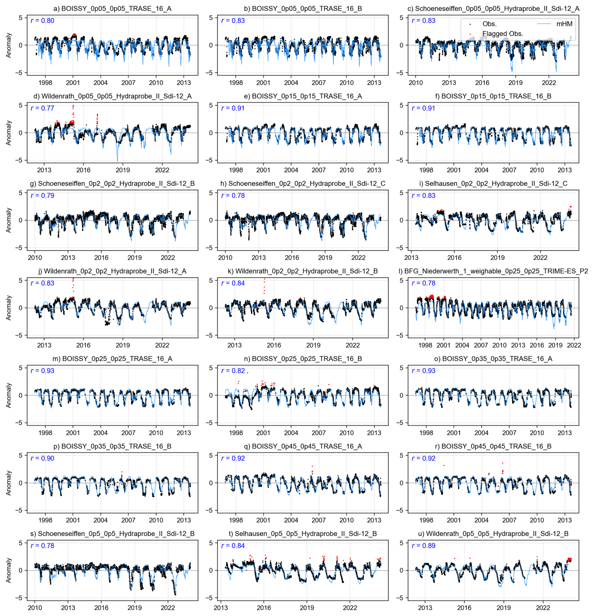
Figure 3 Comparison of standardized anomalies between mHM and in situ soil moisture at selected ISMN sites, ordered by increasing sensor depth. The red scatter points represent observed soil moisture values flagged as potentially erroneous. Titles follow the format station_topdepth_bottomdepth_sensortype, e.g., BOISSY_0p05_0p05_TRASE_16_A refers to the Boissy station with a sensor at 0.05 m depth and sensor type TRASE.

Regarding streamflow performance, the model shows good and spatially consistent skill across the entire modelling domain and thus provides a reliable basis for analysing soil moisture dynamics. We evaluated daily discharge at 168 gauging stations. During calibration, the mean Nash-Sutcliffe Efficiency (NSE) across stations was 0.62, with 80 % of stations achieving NSE ≥ 0.5 (a commonly used benchmark for satisfactory streamflow simulation). Model performance during the validation period was also comparatively good, with a mean NSE of 0.63 and 83 % of stations recording NSE ≥ 0.5. The full details of the streamflow evaluation, including the NSE definition, are provided in Sect. S2 in the Supplement (Fig. S1).

3.2 Decadal evolution of soil-moisture droughts

To summarize how soil-moisture drought behaviour evolves across decades, we use three complementary metrics. First, we quantify the magnitude of each event using the Total Drought Magnitude (TDM), which integrates drought severity over space and time and thus allows drought events to be ranked consistently (Sect. 3.2.1). Second, in Sect. 3.2.2, we describe how drought severity is distributed by quantifying the fraction of drought-affected area falling into different severity classes (moderate, severe, extreme, and exceptional) within each decade. These classes capture shifts in the composition of drought conditions beyond just the total magnitude. Third, in Sect. 3.2.3, we quantify cumulative drought exposure as the total number of months in which each grid cell experiences drought per decade (months need not be consecutive). This metric summarizes how frequently drought conditions recur at a given location over a decade. For decadal summaries, we defined decades starting from 1971 (i.e., 1971–1980, 1981–1990, etc.) since SPEI construction requires accumulated water-balance anomalies over preceding months (January 1970 will thus not have SPEI-1 values, while January–March 1970 lacks SPEI-3 values. The first year with complete SPEI values is 1971).

3.2.1 Magnitude-based ranking of soil-moisture drought events

Figure 4 shows the magnitude of simulated soil moisture droughts in Belgium between 1970 and 2020 based on the Total Drought Magnitude (TDM), the cumulative deficit in soil moisture below the drought threshold (SMI ≤ 0.20), integrated over the affected area and the event duration. To ensure an unambiguous severity ranking, the events are ranked by TDM and when two events have similar TDM (difference <1 %), ranks are resolved using a fixed tie-breaker hierarchy: (i) average drought area (fraction of the domain with SMI ≤0.20 averaged over the entire event), (ii) duration, and (iii) exceptional-class exposure (fraction of SMI ≤0.020 summed over the duration of the event). On the basis of this ranking, Table 2 displays the corresponding metrics for the ten largest droughts during the period of analysis. From an interdecadal perspective, Fig. 4 reveals three distinct drought regimes. Beginning with the 1970s, three major drought events are apparent, dominated by the historic 1975–1977 drought. Although this event is commonly referred to as the 1976 drought, probably because that is when it peaked, the analysis shows that its development in Belgium began back in the autumn of 1975 and lasted for a record 16 months until the winter of 1977. By the end of the event, almost 63 % of the domain had experienced drought conditions, although this fluctuated over time². This event established a benchmark against which subsequent droughts in many parts of Europe are commonly compared. Our analysis reflects this, as this event almost matches the most intense drought in Belgium during the period of our analysis.

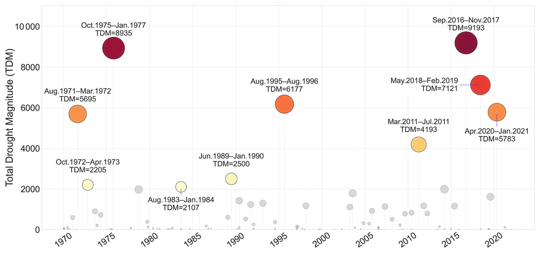
Figure 4 Duration and magnitude of drought events from 1970 to 2020. Each circle represents a drought event, positioned according to its start date (x-axis). The circle size is proportional to the Total Drought Magnitude (TDM) of each event. The 10 most severe droughts, ranked by TDM, are highlighted with coloured markers, with their corresponding periods annotated. Events are ranked primarily by TDM; when two events have similar TDM (difference ≤ 1 %), ranks are determined by peak affected area, then duration, then exceptional-class exposure (defined as SMI ≤ 0.02).

The subsequent three decades (1981–1990, 1991–2000, and 2001–2010) are characterized by a comparatively wetter hydroclimatic regime, reflected in the lower-magnitude drought events in Fig. 4. Only three events from this period appear in the top 10, and all rank relatively low by TDM. The largest of these, the 1995–1996 drought, nonetheless persisted for 13 months.

A significant shift in drought frequency and severity emerged after 2011. Of the 10 biggest droughts from 1971, four of them were recorded between 2011 and 2020, three of which occurred in rapid succession between 2016 and 2020. The 2016–2017 drought is the biggest in this period, exceeding even the 1975–1977 drought by TDM and affected area (64 %) and lasting nearly as long (15 months), as shown in Table 2. The 2018–2019 drought also ranks among the largest events, exceeded in TDM only by the 2016–2017 and 1975–1977 droughts (Table 2). Although it persisted for only 10 months, it affected a large fraction of the domain on average (73 %). Although some big droughts have occurred after 2020, we have excluded these from our inter-decadal analysis because the current decade is still incomplete.

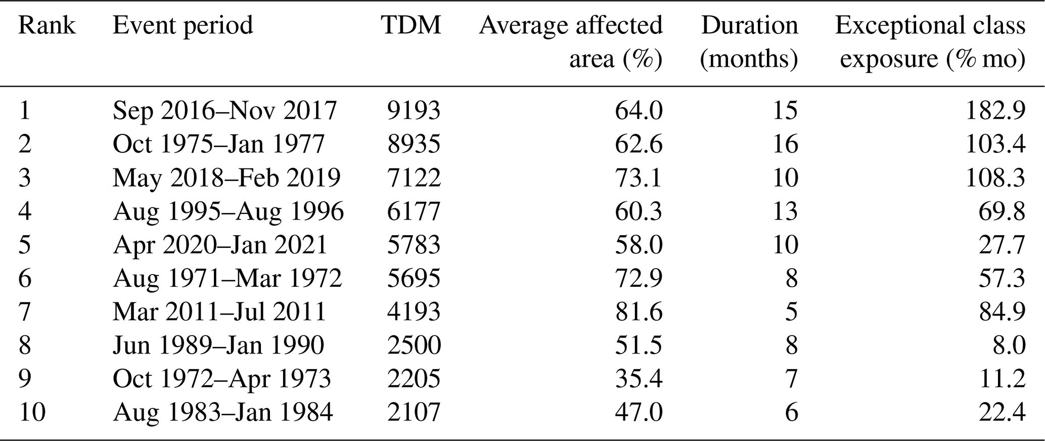
Table 2 The ten biggest soil moisture drought events in Belgium, ranked by Total Drought Magnitude (TDM).

3.2.2 Decadal shifts in drought severity

While TDM provides a suitable event-ranking metric, it aggregates drought conditions over space and time and therefore does not directly indicate whether severity arises from widespread moderate drought or short periods of extreme conditions. To resolve this, we classified all the drought events into four severity classes following Svoboda et al. (2002): moderate drought ($\mathrm{0.1}<\mathrm{SMI}\le \mathrm{0.2}$), severe drought ($\mathrm{0.05}<\mathrm{SMI}\le \mathrm{0.1}$), extreme drought ($\mathrm{0.02}<\mathrm{SMI}\le \mathrm{0.05}$), and exceptional drought (SMI≤0.02). We then examined how the severity of droughts has evolved within and across decades, as shown in Fig. 5. For conciseness we will examine the changes at both ends of the drought severity spectrum.

As Fig. 5 shows, droughts during 1971–1980 were predominantly moderate (0.1 < SMI ≤ 0.2). When exceptional droughts occurred, they remained spatially limited, peaking at below 30 % of the domain during the 1971–1972 and 1975–1977 events (shown by the black dots in Fig. 5). As the figure shows, these two droughts were disrupted by wetter spells, which allowed the re-establishment of normal-to-wet soil moisture conditions between drought phases. When accumulated over the decade, moderate droughts accounted for almost 75 % of all grid-cell months affected by drought, whereas exceptional drought contributed ∼3 %, largely associated with the 1975–1977 event (donut plots in Fig. 5).

Between 1981 and 2010, the drought regime was characterized by predominantly normal-to-wet conditions interspersed with episodic, short-lived droughts. Decadal aggregates indicate that at least 80 % of drought-affected grid-cell months during this period were moderate in intensity, whereas exceptional drought contributed on average less than 1 % (Fig. 6). However, individual events (e.g., the 1995–1996 drought) still exhibited brief peaks of exceptional drought extent when exceptional conditions reached ∼30 % of the domain (Fig. 5).

By contrast, the 2011–2020 period experienced more frequent and severe droughts, particularly towards the end of the decade (Fig. 5). In comparison to the previous decades, the spatial footprint of exceptional droughts noticeably increased. At the peak of the 2011 droughts, exceptional droughts affected close to 70 % of the domain, while during the 2016–2017 drought, about 40 % of the drought-affected area was under exceptional drought, which did not previously occur even during the 1975–1977 event. This increase is reflected in the decadal drought area severity, where exceptional droughts accounted for 5.9 % of the drought-affected area, a proportion that exceeds all the previous four decades combined (Fig. 5).

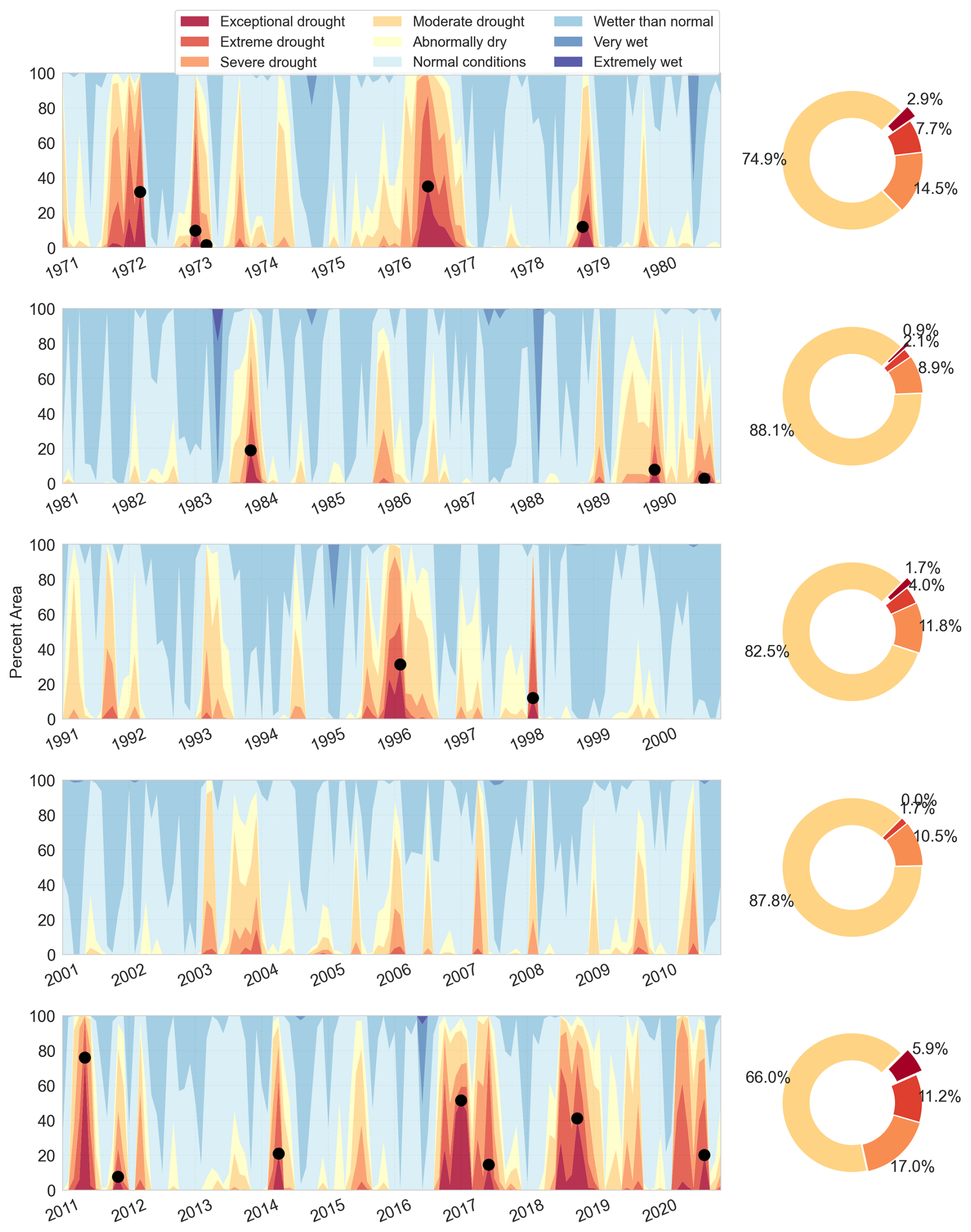
Figure 5 Decadal evolution of drought severity in Belgium, 1971–2020. The stacked panels (left) show the monthly percentage of land area in each soil-moisture class. Black dots mark the peak extent of exceptional drought (SMI ≤0.02). The donut charts (right) summarize, for drought months only (SMI ≤0.20), the mean share of drought-affected area in each drought class; months without drought contribute no area.

3.2.3 Decadal drought exposure

Complementing the temporal and spatial analyses, Fig. 6 illustrates decadal cumulative drought exposure, expressed as the total number of months in which each grid cell experienced SMI ≤ 0.2 in a decade. During 1971–1980, the domain accumulated between 12 and 36 drought months, with a domain-wide mean of about 24 months per grid cell (2.4 months per year) (Fig. 6 inset histogram).

Domain-wide improvements in moisture conditions are apparent in the next three decades. The mean cumulative totals fell to 13 months in 1981–1990 (1.3 months per year), 17 months in 1991–2000 (1.7 months per year), and 14 months in 2001–2010 (1.4 months per year). As with the other metrics, cumulative drought exposure peaked in 2011–2020. The domain accumulated between 24 and 48 months of drought over the decade, and the domain-wide mean rose to 37 months, or 3.7 months per year (Fig. 6). To put this into perspective, this amounts to roughly three continuous years of soil-moisture drought within the decade. This cumulative exposure is more than twice that of each of the three preceding decades (1981–1990, 1991–2000, 2001–2010) and about 1.5 times higher than the previous driest decade, 1971–1980.

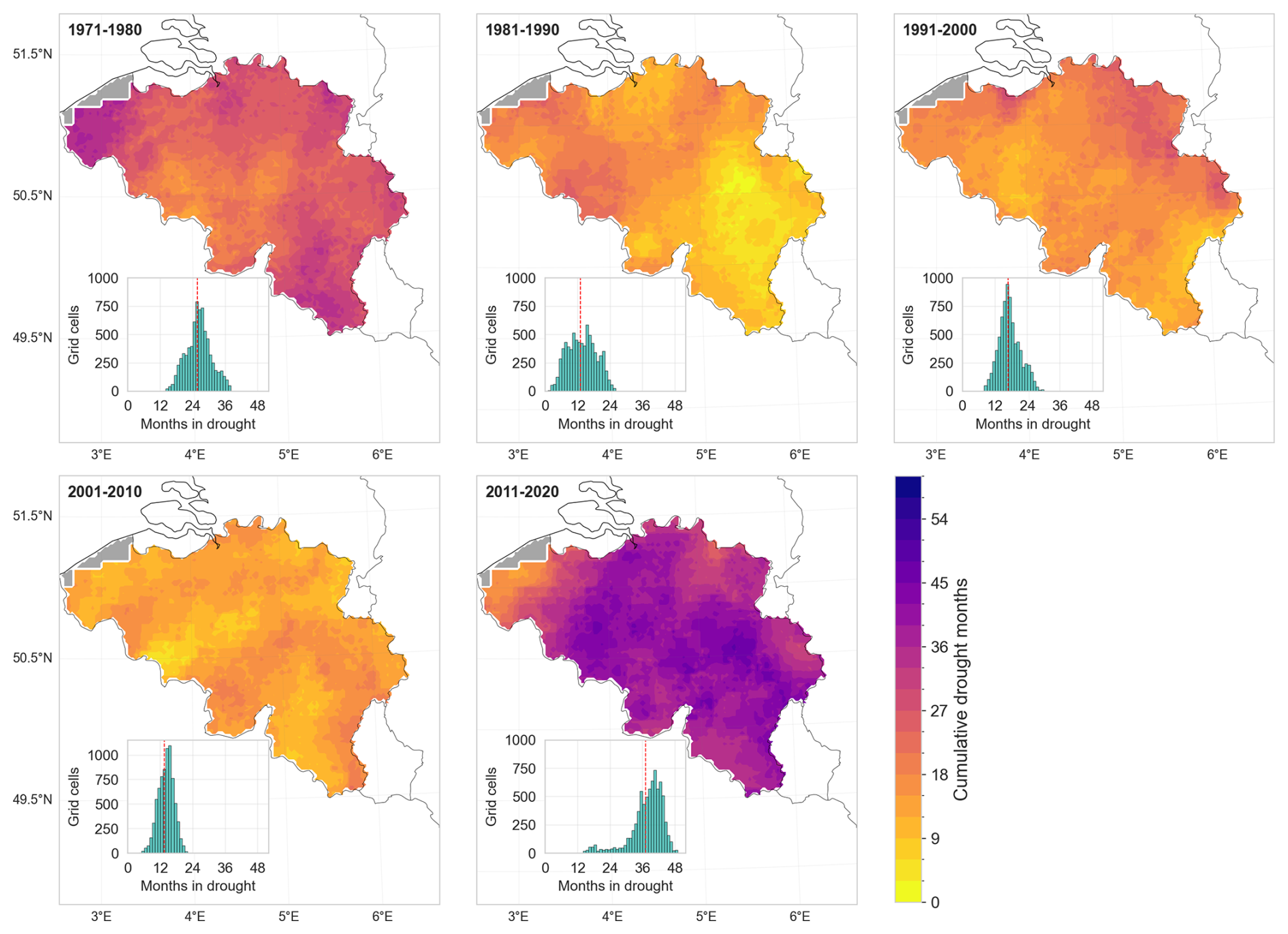
Figure 6 Cumulative decadal drought exposure expressed as the number of months within each decade that a grid cell experienced drought conditions (SMI ≤ 0.2). The inset histograms show the frequency distribution of cumulative time under drought for all grid cells. The red dashed line indicates the mean duration. EOBS data is missing for the region shaded grey.

To test whether 2011–2020 was statistically drier than the preceding four decades, we applied a non-parametric bootstrap to the per-pixel cumulative drought durations (SMI ≤ 0.20) and to the subset of exceptional drought months (SMI ≤ 0.02). For each decade, we generated 100 000 bootstrap samples by resampling grid‐cell drought durations with replacement, calculated the mean for each sample, and used the 2.5th and 97.5th percentiles of the resulting distribution to derive the 95 % confidence interval (CI) of the sample mean.

The statistical analysis concludes that 2011–2020 was indeed the driest decade of the five decades, both in terms of total drought duration and exposure to exceptional droughts. Over the decade, Belgium accumulated a mean drought period of 37 months (CI: 36.9–37.2 months), significantly higher than in 1971–1980 (mean = 25.65 months [CI: 25.6–25.8]), which is the next driest decade (Fig. 7a). The lower bound of the 2011–2020 decade CI lies 11 months above the upper bound of the 1971–1980 period and far higher than those experienced in the three decades in between (1981–1990: mean 13 months [CI: 12.92–13.15], 1991–2000: mean 16.9 months [CI: 16.80–16.95] and 2001–2010: mean 13.52 months [CI: 13.46–13.59]).

A similar contrast emerges for the most severe drought (Fig. 7(b)). The 2011–2020 decade accumulated 4.3 months of exceptional drought on average (CI: 4.28–4.38), more than the combined total of the four earlier decades. None of the previous decades reached a mean of 2 months of exceptional droughts. 1971–1980 accumulated 1.94 months (CI: 1.89–1.98), 1981–1990 only 0.35 months (CI: 0.34–0.36), 1991–2000 0.80 months (CI: 0.79–0.84), and 2001–2010 experienced virtually no exceptional drought. In cumulative terms, more than half of all exceptional drought months in the five-decade record occurred between 2011 and 2020.

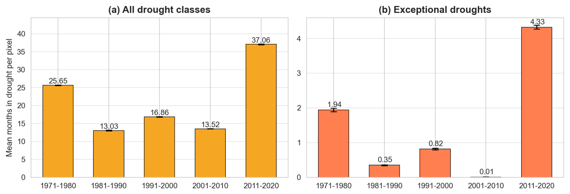
Figure 7 Decadal pixel-wise cumulative drought exposure. The bars show the mean number of months each grid cell spent in drought per decade (not necessarily consecutive), with 95 % bootstrap confidence intervals (black whiskers) for (a) All drought classes (SMI ≤ 0.20) and, (b) exceptional drought only (SMI ≤ 0.02).

3.3 Divergence between soil moisture and SPEI droughts

To examine how precipitation-based drought indicators reflect land-surface moisture stress, we compared SMI and SPEI patterns during the three most severe soil moisture drought events ranked by total drought months (TDM): 1975–1977, 2016–2017, and 2018–2019. Because SMI is computed on a monthly timescale, we derived the climatic water balance (precipitation minus potential evapotranspiration) from E-OBS and calculated SPEI at one- and three-month accumulation periods. Pixel-wise SPEI-1 and SPEI-3 were computed using the SPEI package developed by Vonk (2024). We limited the accumulation period to three months because this timescale is currently used in operational drought monitoring in Belgium. Since SPEI is anomaly-based rather than percentile-based, we associated SPEI $=-\mathrm{1.0}$ with SMI =0.2 to represent the threshold for at least moderate drought, following the drought severity guidelines of Svoboda et al. (2002). We evaluated the differences between indices in terms of (i) anomaly magnitude, (ii) drought persistence (maximum number of consecutive months under at least moderate drought within an event), and (iii) cumulative drought exposure (total number of months, not necessarily consecutive, under at least moderate drought within the event window).

In terms of anomaly magnitude, SMI generally indicated stronger and longer-lasting deficits than SPEI-1 and, to a lesser extent, SPEI-3 (Fig. 8). SPEI-1 responds strongly to short-lived precipitation anomalies that may not immediately translate into changes in root-zone storage. By design, SPEI-3 smooths some of the short-term variability in SPEI-1 and more closely resembles the temporal evolution of soil-moisture anomalies, but still tends to underestimate deficit magnitude relative to SMI over our domain (Fig. 8). Among the three events, SMI indicated the strongest soil moisture deficits during 2016–2017 (with SMI approaching zero), which is not reflected in either SPEI-1 or SPEI-3. Although the 2016–2017 drought was interrupted by intermediate wet conditions during March and April 2017, leading to partial recovery, this wet spell did not split the event because the month-to-month overlap in drought area remained above the 640 km² merging threshold, and the drought therefore remained a single multi-temporal event.

We also found that SMI-based droughts exhibited higher persistence than SPEI-based droughts. Median persistence for SMI was 9 months in 1975–1977, 6 months in 2016–2017, and 7 months in 2018–2019 (Table 3). In comparison, SPEI-1 shows much shorter median persistence (3 months in 1975–1977 and 2 months in both 2016–2017 and 2018–2019), while SPEI-3 is closer to SMI but remains lower (7 months in 1975–1977 and 5 months in both 2016–2017 and 2018–2019).

The same pattern is evident for cumulative drought exposure. Median cumulative exposure for SMI was 10 months in 1975–1977 and 2016–2017 and 8 months in 2018–2019, compared with 4, 6, and 3 months for SPEI-1 and 7, 8, and 6 months for SPEI-3 (Table 3, additional maps in Sect. S3 in the Supplement, Figs. S3 and S4).

This systematically longer persistence and exposure shown by the SMI indicates that soil moisture droughts last longer than precipitation-based droughts because transient precipitation events do not necessarily translate into root-zone recovery. Additional description on the patterns of SMI and SPEI recovery is presented in Sect. S3 in the Supplement.

The differences presented herein do not imply that one indicator is necessarily better; rather, they are all useful for demonstrating how a drought shock progressively propagates through different components of the hydrological system. Precipitation-based indices like SPEI reflect short-term meteorological inputs that may still be agriculturally meaningful. As Fig. 8 shows, rainfall events during dry periods may not replenish deeper soil moisture due to immediate losses through evapotranspiration, yet these events can still temporarily alleviate plant water stress, especially for fast-responding, shallow-rooted crops or annual crops. The recovery of SPEI out of drought conditions may thus signal “relief” that is real, albeit short-lived and limited in scope. On the other hand, SMI-based drought analysis better captures the persistence of land surface water deficits and the residual moisture stresses that continue to affect the dependent ecosystems (e.g., perennial deep-rooted vegetation) long after meteorological conditions have normalized.

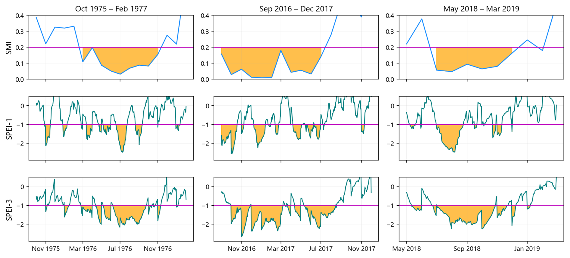
Figure 8 Comparison of domain-average SMI, SPEI-1, and SPEI-3 time series during the three biggest drought events up to 2020. The orange shaded areas indicate drought conditions, defined as SMI ≤ 0.2 and SPEI ≤ -1.0. The horizontal magenta lines mark the drought threshold for each index.

Table 3 Domain-wide median persistence and cumulative drought exposure for the events in Fig. 8, based on SMI, SPEI-1, and SPEI-3.

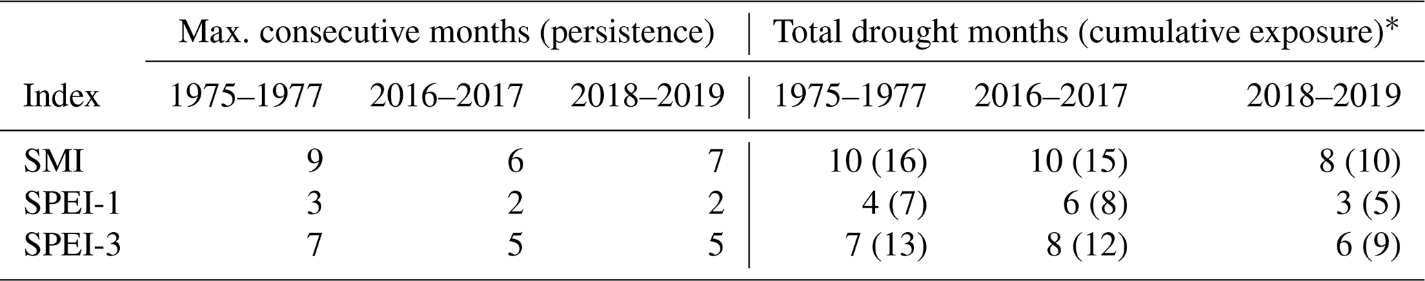
^∗ Values in parentheses denote the maximum cumulative exposure until all pixels emerge out of drought.

4 Discussion

This extended temporal analysis of soil moisture droughts over Belgium offers new insights on the severity of recent droughts in the country. Using multiple drought metrics, we show that the 2010s were characterized by significantly greater drought exposure, duration, and severity than the preceding four decades since 1970. Our findings fit into the wider pan-European narrative of intensifying droughts over the continent in the 21st century. García-Herrera et al. (2019) showed that the 2016–2017 drought in central-western Europe was among the most severe events in the recent observational record. Longer-term reconstructions further indicate that the succession of European summer droughts between 2015 and 2018 was exceptional even in a millennial context (over the previous 2110 years) (Hari et al., 2020; Büntgen et al., 2021; Rakovec et al., 2022). This recent intensification of droughts has been attributed to a combination of persistent atmospheric blocking and anthropogenic warming, which together reduce moisture supply and enhance evapotranspiration (Ionita et al., 2020; García-Herrera et al., 2019; Hari et al., 2020). Under continued warming, these conditions are projected to increase the frequency and severity of similar magnitude droughts (Samaniego et al., 2018; Hari et al., 2020; Rakovec et al., 2022).

On the comparison between precipitation and soil-based drought indicators, we stress that these indicators are useful for different components of the hydrological system. SPEI-1 and SPEI-3 may suit analyzing drought patterns in shallow soil layers and shorter temporal scales but are limited for indicating drought persistence deeper in the soil or in complex ecosystems due to their ignorance of land-ecosystem interactions (Xu et al., 2021; Peng et al., 2024). When assessing drought impacts on ecosystems, groundwater recharge, or perennial vegetation like forests, the divergence between meteorological and soil moisture signals can become complex. In such systems, soil properties such as hydrophobicity during prolonged dry periods can lead to highly uneven infiltration (Gimbel et al., 2016; Filipović et al., 2018). Heavy summer rainfall may not be absorbed uniformly across the soil profile but instead run off or infiltrate preferentially along cracks, roots, or macropores, sometimes bypassing the upper root zone. While this limits the ability of standard soil moisture indices to reflect actual water availability near the surface, it may still benefit deep-rooted vegetation like trees by replenishing deeper soil layers (Zhu et al., 2015; Duniway et al., 2018). Assessing drought stress and recovery in these systems thus requires models and indicators that account for vertical and spatial heterogeneity in infiltration and root water uptake (e.g., Shen et al., 2025), rather than relying solely on averaged or surface-weighted soil moisture metrics. Further, while it may be argued that SPEI at longer accumulation periods (e.g., 6, 9 or 12 months) can lead to a closer resemblance of root-zone moisture conditions, finding the appropriate accumulation lengths is dependent on landscape and soil characteristics (topography, rooting depth, soil hydrology and management conditions) and climatic conditions, which can lead to a strong variation of drought characteristics if the landscape is heterogeneous. Kumar et al. (2016) indeed found that applying spatially variable accumulation periods achieves a higher correlation between precipitation-based and groundwater drought indices over a uniform domain-wide accumulation period, even at long accumulation times.

Our findings are relevant beyond Belgium because the workflow used in this study can be transferred to other regions provided that the meteorological forcing is available at appropriate resolution, a hydrological or land-surface model is parameterized to represent soil-water storage, and consistent long-term simulations can be produced. Extending the analysis to other domains would allow the same drought dynamics addressed in this study to be evaluated under different climate gradients, soil, land-cover conditions, and management regimes.

From an operational perspective, the results support a monitoring strategy that complements precipitation-based indices with soil-moisture-based indicators rather than interchanging them. As we have shown, precipitation-based indices are useful for tracking meteorological anomalies and can provide early signals of emerging drought risk, but they may not capture persistent impacts when land-surface memory sustains root-zone deficits after rainfall resumes. In an operational system, precipitation-based indices can be used for early warning, while a root-zone soil moisture drought indicator is better utilized to track agricultural drought development and recovery and to assess when conditions have returned to normal in the soil profile. These outputs can be integrated into management decisions by linking drought phase and persistence to sector-relevant decisions. For example, soil-moisture drought persistence is directly relevant for agricultural advisories that inform planting and irrigation planning and signaling crop yield risk and the risks associated with the occurrence of wildfires or floods that can occur due to seasonally saturated soils. Slow recovery in soil and catchment storage after meteorological drought can also inform water supply preparedness and groundwater management, since water resources often show a delayed return to normal conditions (Yang et al., 2017). For inland navigation and low-flow management, combining soil moisture drought information with streamflow indicators can help distinguish short, transient precipitation deficits from longer-lasting, storage-driven drought conditions. In practice, monthly updates of a root-zone soil moisture drought map, paired with precipitation-based indices, would support earlier identification of drought evolution and lead to more realistic expectations for recovery following intermittent wet periods (Van Loon et al., 2024).

5 Limitations and future work

Our results rely on the evaluation of model-derived soil moisture conditions, which are inevitably constrained by structural, parametric, and forcing uncertainties that we did not explicitly evaluate. Choices of the mapping between drought categories (e.g., SPEI $=-\mathrm{1.0}$ vs. SMI ≤0.2) and a uniform accumulation period over the whole domain (for SPEI analysis) also introduce additional subjectivity. The mHM model also does not account for anthropogenic factors such as irrigation, groundwater abstraction, tile drainage and artificial canals, and land management conditions, which affect the hydrology of the domain. Future work can partially offset these limitations by quantifying uncertainty using ensembles of forcings, investigating model parameters to derive confidence intervals for drought magnitude, area, and timing, incorporating human water use and irrigation processes, or assimilating independent observations (such as in situ or remotely sensed soil moisture and terrestrial water storage) to better constrain states and evaluate the joint behaviour of multiple drought indicators alongside observed impacts.

6 Conclusions

This study provides a multi-decadal, high-resolution reconstruction of root-zone soil moisture droughts over Belgium from 1970 to 2020. Using event-based severity metrics that quantify drought duration, spatial extent, and intensity, we show that 2011–2020 was marked by substantially greater cumulative drought exposure than any preceding decade, exceeding the previous driest decade by about 1.5 times. The 2011–2020 decade also exhibited the highest share of exceptional drought, with cumulative exceptional drought exposure exceeding that of all earlier decades combined.

By comparing soil-moisture drought (SMI) with precipitation-based indicators (SPEI-1 and SPEI-3) for the three most severe events, we show that precipitation-based indices systematically underestimate drought persistence and cumulative exposure relative to root-zone soil moisture. In particular, soil moisture droughts persist longer and recover more slowly than meteorological anomalies, reflecting land-surface memory. Including soil moisture monitoring in drought observatories thus offers the added value of capturing lingering stresses on agriculture and ecosystems, which can persist long after meteorological conditions have normalized. This provides decision-makers with a more complete view of drought severity and duration and supports targeted response and mitigation efforts.

The reconstructed drought record and event-based metrics presented in this study provide a consistent basis for benchmarking recent droughts against historical variability and for supporting drought monitoring and management.