Multivariate calibration can increase simulated discharge uncertainty and model equifinality

Hydrological models are typically calibrated against discharge data. However, the resulting parameterization does not necessarily lead to a realistic representation of other variables, and multivariate model calibration may overcome this limitation. It seems reasonable to expect that multivariate calibration leads to reduced hydrograph uncertainty, associated with more constrained flux maps (i.e., combinations of streamflow generation mechanisms). However, this expectation assumes that an intersection exists within the parameter space between the separate behavioural clouds of the two or more variables considered in multivariate calibration. Here, we tested this assumption in twelve Australian catchments located in five different climate zones. We calibrated the SIMHYD model using a Monte Carlo-based approach in which an initially large sample of parameter sets was constrained using discharge only, actual evapotranspiration only, and a combination of both variables (i.e., a single combined objective function). We demonstrated that adding actual evapotranspiration to a discharge-based calibration caused hydrograph uncertainty to increase for 11 of the 12 sites. Similarly, flux maps became less constrained under multivariate calibration relative to univariate calibration. Analysis of behavioural parameter sets suggests that these symptoms could be caused by non-overlapping behavioural parameter distributions among the different variables. By separately considering both locally observed and remote sensing-based evapotranspiration in the analysis, we could demonstrate that the source of the information did not affect our findings. This has implications both for model parameterization and model selection, emphasising that the value of non-discharge data in calibration is contingent on the suitability of the model structure.

1 Introduction

Nearly all hydrological models have parameters that cannot be directly measured and need to be calibrated. In calibration, model parameter values are estimated so that the model can closely match the observed hydrological behaviour of a catchment. Calibration is typically based on discharge, which is an integrated signal of the catchment response. For a given model, calibration with discharge can lead to several parameter sets with similar discharge response (known as equifinality; Beven, 2006). However, these parameter sets can reach a similar discharge response through different model pathways and not all of them realistically represent hydrological stores and fluxes other than discharge (Bouaziz et al., 2021; Khatami et al., 2019; Pool et al., 2024; Rakovec et al., 2016).

One way to improve process representation in hydrological models and thus their physical realism is to estimate model parameter values using complementary data in addition to discharge (Efstratiadis and Koutsoyiannis, 2010). These could, for example, include in-situ or remote sensing-based observations of actual evapotranspiration (Arciniega-Esparza et al., 2022; Meyer Oliveira et al., 2021; Széles et al., 2020), soil moisture (López López et al., 2017; Mei et al., 2023; Stisen et al., 2018), groundwater levels (Kelleher et al., 2017; Pleasants et al., 2023; Seibert and McDonnell, 2002), or total water storage (Dembélé et al., 2020a; Demirel et al., 2019; Nijzink et al., 2018).

Improvements in model realism are often quantified in terms of model performance for different hydrological variables. Considering a non-discharge variable (such as actual evapotranspiration) in addition to discharge in model calibration strongly improves model performance for that particular variable, while the performance for discharge is typically deteriorated (Livneh and Lettenmaier, 2012; Mostafaie et al., 2018; Yassin et al., 2017). Using a large sample of catchments in Australia, Pool et al. (2024) showed that such trade-offs between discharge and the other variables get more pronounced with increasing catchment wetness. However, there may be benefits for other variables not used in calibration, with recent work by Dembélé et al. (2020a) in the Volta Basin and Mei et al. (2023) in catchments in the United States showing the presence of cross-benefits meaning that the use of a particular variable in calibration also leads to more realistic simulations of other variables not used in calibration.

It is also common to evaluate model realism by considering the behavioural parameter space. An example is the use of reduced parameter uncertainty to indicate improved process representation in hydrological models (Blazkova et al., 2002; Rajib et al., 2016; Zink et al., 2018). Ideally, there is a physically meaningful link between the parameters with improved identification and the calibration variables, such as better constrained soil parameter values when adding actual evapotranspiration to a discharge-based calibration (Arciniega-Esparza et al., 2022; Demirel et al., 2019). Another parameter-based indicator is the final number of parameter sets considered behavioural in Monte Carlo-like calibration approaches (an indicator of the size of the behavioural subspace). For example, Hartman et al. (2017) started from a large initial sample of randomly generated parameter sets and selected behavioural parameter sets based on performance thresholds. Model performance was measured using an objective function for discharge only or by simultaneously evaluating discharge and water quality data with two separate objective functions, and the latter produced less behavioural sets. Similar conclusions were reached by Arciniega-Esparza et al. (2022) and Kelleher et al. (2017) who used multiple hydrological variables, each evaluated with an individual objective function, and a step-wise or hierarchical selection of behavioural parameter sets. Such approaches assume that a calibration with a single variable leads to many equifinal parameter sets that cover a relatively large area of the parameter space, which can then be further constrained using additional variables. While several studies have reported that multivariate parameter selection results in a much smaller sample of behavioural parameter sets than selection with a single variable, few studies address the possibility and implications of constraining to the point where the subspace disappears entirely (i.e., no intersection), an eventuality that is discussed further below.

At the broadest level, there are two common ways of looking at multivariate calibration, only one of which is in focus here. The first is that the two (or more) variables are in competition with one another and thus are “traded-off”, or alternatively are weighted in accordance with their perceived importance so that a single “optimal” solution can be identified (as opposed to a set of Pareto-optimal candidates). This paradigm is not the focus in this paper. The other way of looking at multivariate calibration is as a restricting of the behavioural parameter space, as discussed above. By behavioural, we mean model simulations are consistent with observations to some standard of performance (an acceptance threshold), where both the performance metric and the acceptance threshold may be subjectively chosen. The behavioural parameter space, then, is the cloud of parameter sets that meet or exceed the acceptance threshold. In this view, multivariate calibration is a way of making the cloud smaller, whereby the goal is to seek the intersection between the separate behavioural clouds of two or more variables. It seems reasonable to assume that such an intersection exists, and having made this assumption, it follows that the intersection is smaller than the individual clouds. Thus, restricting parameter sets to only those within the intersection should reduce the uncertainty in simulations. To be clear, we are not criticizing this view here – indeed, we feel it is advantageous in that it treats the information in the separate variables as complementary and beneficial.

However, one limitation of the latter view is the assumption that the clouds intersect – this assumption is rarely mentioned, let alone explicitly tested. A lack of intersection might be a symptom of problems such as an inadequate model structure (Beck, 2005; Fowler et al., 2020; Wagener, 2003) or data that are subject to systematic biases or other errors (Beven and Westerberg, 2011; Girons Lopez and Seibert, 2016). If no intersection exists, it is possible that the application of multivariate calibration may result in the following perverse and rarely reported outcomes: either (i) zero behavioural parameters sets, in which case presumably the modelling exercise must be altered or abandoned; or (ii) multivariate calibration might cause uncertainty to increase, rather than decrease - this could happen if the assessment of parameter set performance is done jointly across variables, such as where a large random cloud is generated and a selection is chosen based on aggregate performance across variables. In this case, the method is agnostic to the presence or absence of an intersection since it will return a result either way. This latter case is demonstrated in this paper.

There are, however, some exceptions to the above generalizations. It is admittedly more common for studies to focus on model performance than uncertainty, and studies focusing on uncertainty sometimes report mixed results. For example, taking a discharge-based calibration as reference, Gallart et al. (2007) reported a more constrained hydrograph in the Can Vila catchment (Catalan Pyrenees) when considering discharge and water table data in calibration, Blazkova et al. (2002) found no significant improvements for the Uhlirska catchment (Czech Republic) when simultaneously using discharge and maps of saturated area, and Lamb et al. (1998) found wider discharge uncertainty bounds in the Minifelt catchment (Norway) for a calibration with discharge and water table data. Nor is the uncertainty in the hydrograph or in parameter values the only way to express uncertainty or equifinality. Recently, Khatami et al. (2019) suggested Flux Mapping to evaluate model equifinality and realism of process representations in models (see also Sect. 2.3.3). A flux map is a plot showing how much different model internal fluxes contribute to total simulated discharge. In their example, they used a model in which discharge is the result of three runoff generating processes (i.e., overland flow, interflow, and baseflow). The flux map was visualized as a ternary plot where each axis showed the contribution of one of the three model internal fluxes. Plotting results from many model simulations creates a map of the modelled catchment behaviour. Their results for several Australian catchments showed that very different flux combinations can be active for a narrow range of model performance, suggesting equifinality of runoff fluxes. Thus, flux maps characterize equifinality by considering variation in contribution between three simulated runoff generating processes (i.e., overland flow, interflow, and baseflow), possibly providing an interesting alternative lens through which to assess the effect of multivariate model calibration.

In summary, based on previous work, we may conclude that many modelers (including, until recently, the authors of this study) would expect that adding complementary data to a discharge-based calibration leads to a more constrained parameter space and an improved overall process representation. Consequently, a modeler could assume that the model internal runoff flux space is more constrained leading to a reduced uncertainty of hydrograph simulations. Here, we test these two assumptions using the following hypotheses:

• H1: Adding complementary data to a discharge-based model calibration reduces model equifinality, leading to more constrained clouds of behavioural parameter sets and model internal flux maps.

• H2: Hydrograph uncertainty is reduced when adding complementary data to a discharge-based model calibration.

With these two hypotheses we explicitly focus on hydrograph uncertainty and runoff flux maps, which complements existing multivariate calibration studies that tend to focus their attention on model performance.

We tested the two hypotheses in twelve Australian catchments located in five different climate zones. We used the SIMHYD model, which, while conceptual in nature and spatially lumped, explicitly simulates different runoff processes and is thus a suitable choice to explore using flux maps as well as considering traditional (parameter and simulation) uncertainty. We calibrated SIMHYD for each catchment using discharge only, actual evapotranspiration only, and a combination of both variables. The twelve study catchments are located near flux tower monitoring sites, which allowed us to separately consider both locally observed and remote sensing-based evapotranspiration to determine if the source of the information influenced the outcome. Using these data, we demonstrate that multivariate model calibration can increase equifinality in simulated flux maps and uncertainty in hydrograph simulations. We show that these symptoms co-occur with non-overlapping behavioural parameter distributions for the individual calibration variables, suggesting a possible causative link. The consequence is that non-discharge data may have little value unless the model structure is suitable, which indicates that modelers should be cautious when using legacy-based approaches to model selection (Addor and Melsen, 2019) and instead apply more rigorous and holistic evaluation approaches across a wider pool of candidate models. Thus, this study has implications both for model selection and for methods currently used to calibrate models for practical applications and decision making.

2 Materials and methods

2.1 Study area and data set

The study was based on twelve Australian catchments with minimal water resource development and land use disturbances. Although larger samples are desirable, here we restrict ourselves to sites that have nearby flux towers to quantify actual evapotranspiration, as discussed below. The catchments cover five Köppen–Geiger climate zones (Peel et al., 2007) and different hydroclimatic regimes (Fig. 1). The tropical catchments in the North have summer-dominated precipitation and discharge regimes arising from monsoon rainfall from January–March (Fig. 1b–d). The arid catchments in northern Australia also have some summer precipitation, but only little results in discharge due to high summer evapotranspiration rates (Fig. 1b–d). Most of the temperate catchments are in the Southeast and Southwest of Australia and for many of them precipitation and discharge is more evenly distributed over the year than in the tropical and the arid catchments (Fig. 1b–d). Overall, mean annual values of precipitation and discharge for the twelve study catchments range from 510–3200 mm, and 12–1720 mm, respectively. The catchments vary in size from 96–4794 km² and are located between 39 and 902 m a.s.l. (meter above sea level).

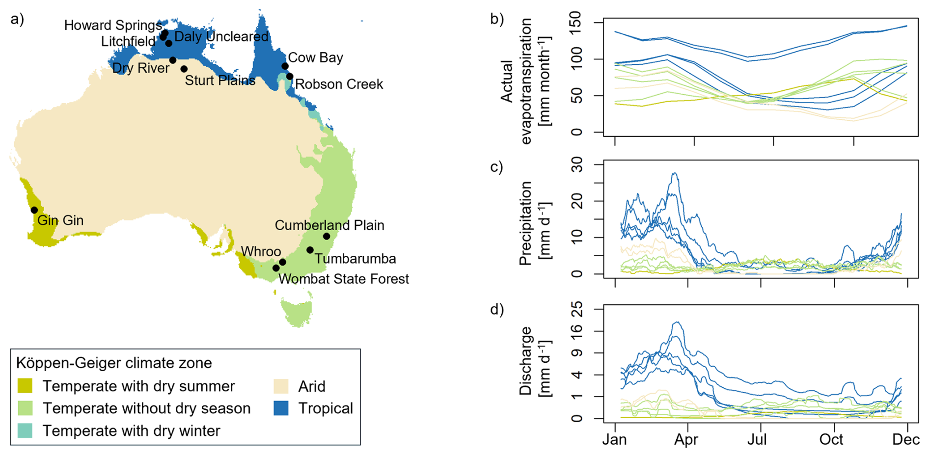
Figure 1 Location and characteristics of the twelve study catchments. (a) Location and Köppen–Geiger climate zone (Peel et al., 2007) of the study catchments. (b–d) Regime curves for actual evapotranspiration (remote-sensing based data), precipitation, and discharge. The regime curve is calculated as the mean value at each day of the year using the hydrological years 2004–2013. Regime curves were smoothed with a fifteen-day moving average.

Daily meteorological and discharge time series were extracted from version 2 of the CAMELS-AUS dataset (Fowler et al., 2024). It provides for all twelve study catchments data from at least 1977–2022. Among the multiple options provided within CAMELS-AUS, we chose the meteorological time series representing catchment averages calculated from the gridded precipitation product ($\sim \mathrm{5}\mathrm{km}\times \mathrm{5}\mathrm{km}$) of Evans et al. (2020) and the gridded Morton's wet environmental areal potential evapotranspiration estimates ($\sim \mathrm{5}\mathrm{km}\times \mathrm{5}\mathrm{km}$) of Jeffrey et al. (2001).

Actual evapotranspiration time series were used from two different sources to consider both remote sensing-based data and locally observed field data. The remote sensing-based time series were retrieved from the global gridded product ($\sim \mathrm{8}\mathrm{km}\times \mathrm{8}\mathrm{km}$) of the Numerical Terradynamic Simulation Group (NTSG) at the University of Montana (Zhang et al., 2010), which is available for the years 1982–2013. Their estimates of monthly actual evapotranspiration are based on biome-specific transpiration and soil evaporation calculated from a modified Penman–Monteith equation. For our study, we calculated a monthly catchment average value using the area-weighted mean of all grid cells covering a particular catchment. The catchment boundaries were taken from the CAMELS-AUS v2 dataset. The dataset was chosen because it has been a commonly used product in Australia (Gardiya Weligamage et al., 2023).

The locally observed time series of actual evapotranspiration were obtained from the OzFlux Research and Monitoring network (Beringer et al., 2016), part of the international Fluxnet program (Baldocchi et al., 2001), which maintains tower-based eddy covariance systems to collect data on energy, carbon, and water fluxes in Australia and New Zealand. Not all OzFlux sites are located within the boundaries of catchments with discharge gaugings. Thus, we matched each of the twelve OzFlux sites used in this study with the catchment having the closest catchment centroid within CAMELS-AUS v2. Table S1 in the Supplement provides the OzFlux site name and the corresponding catchment ID in the CAMELS-AUS dataset. The field-based daily actual evapotranspiration values were transferred to the catchments without modification assuming that they are a reasonable estimate of catchment average evapotranspiration (note that the objective function used is insensitive to bias, for reasons discussed in Sect. 2.3.1). The length of the available time series varies among the twelve OzFlux sites, spanning the most recent 7–21 years.

The temporal coverage differs between the three datasets described above, whereby the time periods of the remote sensing-based and field-based actual evapotranspiration datasets don't overlap. To make modelling results from the two actual evapotranspiration products more comparable, we created two separate model evaluation datasets using the following criteria: (i) the data period should ideally cover ten years, and (ii) only hydrological years with a complete discharge and actual evapotranspiration record are used. The start of the hydrological year depends on the hydroclimatic conditions of a catchment and was defined as the month with lowest average long-term monthly discharge (Wasko et al., 2020). A hydrological year was considered complete if less than 5 % of time steps were missing. As a result, the first model evaluation dataset (D_ETa.RS) including meteorological data, discharge, and remote sensing-based actual evapotranspiration covered the period 2003–2014 with nine out of twelve catchments having the full ten-year record. The second model evaluation dataset (D_ETa.Field) including meteorological data, discharge, and field-based actual evapotranspiration broadly covered the period 2011–2022. Time series length for the twelve catchments ranged between three and ten years with five out of twelve catchments having ten years of data.

2.2 Hydrological model

SIMHYD is a lumped bucket-type hydrological model that has been applied in different hydroclimatic regions of Australia (Chiew et al., 2002; Fowler et al., 2020; Khatami et al., 2019). The model takes daily precipitation and potential evapotranspiration as inputs and simulates a catchment's rainfall–runoff response using three stores and seven parameters (Fig. S1 in the Supplement). The three stores represent interception by vegetation, soil water, and groundwater. The model parameters affect how the state of the stores varies as a function of rainfall, actual evapotranspiration, infiltration, recharge, and runoff generation. The streamflow generation mechanisms modelled by SIMHYD are infiltration excess flow, interflow and saturation excess flow, and baseflow. The three streamflow generation mechanisms are hereafter referred to as overland flow, interflow, and baseflow, and are used to create the runoff flux maps. A more detailed description of SIMHYD can be found in Chiew et al. (2002). The model code for SIMHYD is publicly available from the Modular Assessment of Rainfall–Runoff Models Toolbox (MARRMoT). We used MARRMoT version 2.1 (Trotter et al., 2022).

2.3 Modelling experiment

We defined three calibration cases to systematically analyse the impact of multivariate model calibration on simulated runoff generation and hydrographs. Note that we use the word “calibration” here to denote the process of selecting an ensemble of parameter sets based on their match with observed data. This is different to common usage in which a single “optimum” parameter set, not an ensemble, is chosen. The three calibration cases included a calibration to (i) daily discharge only, (ii) monthly actual evapotranspiration only, and (iii) a combination of both variables. Below we describe the objective functions used in calibration, followed by the calibration process in which parameter values were estimated, and the analysis of the modelling results.

2.3.1 Objective functions

The objective functions used in calibration differed for discharge and actual evapotranspiration and were chosen based on recent work conducted with SIMHYD in Australian catchments. Discharge simulations were evaluated using an objective function O_Q that is designed to ensure that high flows and the very low flows often occurring in some of the study catchments are well simulated while minimizing total volume bias (Trotter et al., 2023). The objective function O_Q is defined in Eq. (1), whereby KGE is the Kling–Gupta efficiency (Gupta et al., 2009) once calculated using direct flows (KGE) and once using the fifth root of the flows (KGE_0.2), and B is the volume bias.

$$\begin{array}{}\text{(1)}& O_Q=\mathrm{0.5}(\text{KGE}+{\text{KGE}}_{\mathrm{0.2}})-\mathrm{5}\times \left|\ln \right(B+\mathrm{1}){|}^{\mathrm{2.5}}\end{array}$$

Simulated actual evapotranspiration was evaluated with an objective function O_ETa that emphasizes small to medium fluxes (Gardiya Weligamage, 2024). Additionally, the chosen objective function explicitly does not evaluate volume bias as many evapotranspiration products suffer from considerable volume bias. This is true both for remotely sensed products, where the bias arises from the uncertainty in converting observable radiation into evaporative fluxes (Elnashar et al., 2021; Wartenburger et al., 2018; Zhang et al., 2020) and in the case of flux towers where bias may arise because the flux tower ET is not representative of the catchment as a whole. In both cases, we assume here that the temporal pattern of ET (as captured by the variability and correlation components of the KGE) is valid as a calibration target even if the overall timeseries is biased too high or too low (Pool et al., 2024). The objective function used to compare simulated with observed actual evapotranspiration is defined in Eq. (2) – it is the Kling–Gupta efficiency without the bias component, whereby r is the linear correlation coefficient between simulated and observed values and α is the relative variability in the simulated and observed values. The two components r and α are calculated on square root-transformed fluxes.

$$\begin{array}{}\text{(2)}& O_{\text{ETa}}=\mathrm{1}-\sqrt{(r-\mathrm{1}{)}^{\mathrm{2}}+(\mathit{\alpha }-\mathrm{1}{)}^{\mathrm{2}}}\end{array}$$

When using both discharge and actual evapotranspiration in model calibration, the objective functions O_Q and O_ETa were combined using the Euclidean distance (Eq. 3).

$$\begin{array}{}\text{(3)}& O_{Q,\text{ETa}}=\mathrm{1}-\sqrt{(O_Q-\mathrm{1}{)}^{\mathrm{2}}+(O_{\text{ETa}}-\mathrm{1}{)}^{\mathrm{2}}}\end{array}$$

2.3.2 Model calibration

For model calibration, we chose a Monte Carlo-based approach in which calibration was used to constrain an initially large sample of parameter sets. By keeping a predefined number of best performing parameter sets for each calibration case, one can evaluate model uncertainty under different data considerations. More specifically, we started model calibration by drawing an initial sample of 100 000 parameter values from a predefined uniform parameter distribution (Peel et al., 2000) using Latin Hypercube Sampling. For each catchment, the model was set up with a two-year warm-up period and then run with each parameter set using the daily meteorological input from the D_ETa.RS model evaluation dataset. The resulting 100 000 simulations were evaluated against observed discharge and actual evapotranspiration using the objective functions O_Q, O_ETa, and O_Q,ETa. In a final step, the 100 best performing parameter sets were selected for each calibration case. We repeated the identical procedure for the second model evaluation dataset D_ETa.Field. Note that for the purpose of this study the entire evaluation dataset was used for calibration and no evaluation in an independent period was conducted.

2.3.3 Flux map and hydrograph uncertainty

A flux map is a ternary plot where each axis represents a streamflow generation mechanism that is simulated in the model (Khatami et al., 2019). For the SIMHYD model, a point on the flux map shows the contribution of overland flow, interflow, and baseflow to total streamflow for a particular model run. Here, we plotted the flux contributions of all 100 best simulations. Cloud patterns filling a large space on the flux map indicate higher degrees of model flux equifinality. We quantified the fraction of the flux map area filled after calibration by calculating the fraction of triangles (i.e., flux map grid cells) covered by the 100 best simulations. The flux map grid was created by dividing each axis into increments of ten percent, resulting in 100 grid cells. The size of the increments is identical for the area quantification as for the visualisation of the map.

Hydrograph uncertainty was defined as the range in discharge values simulated by the 100 best parameter sets at each time step. To investigate uncertainties in different parts of the hydrograph, we calculated uncertainty at different flow quantiles ranging from Q5 (low flow) to Q100 (high flow). The use of flow quantiles rather than absolute flow values made the results for catchments with different hydroclimatic regimes more comparable.

3 Results

As mentioned, the impact of adding complementary data to a discharge-based model calibration was explored for two different datasets, the first using discharge and remote sensing-based actual evapotranspiration (D_ETa.RS) and the second using discharge and field-based actual evapotranspiration (D_ETa.Field). The results and the conclusions from the two datasets were similar and for reasons of brevity, results for the first dataset (D_ETa.RS) are presented in detail, while the results for the second dataset (D_ETa.Field) can be found in Figs. S6–S13 in the Supplement.

3.1 Effect of adding complementary data to a discharge-based model calibration

Significant differences were found in terms of model performance when calibrating with discharge only versus discharge and evapotranspiration (Fig. 2; for more details see also Fig. S2 in the Supplement). The 100 best parameter sets selected in the discharge-based calibration clearly outperformed the uncalibrated model (i.e., median of all randomly sampled parameter sets) when evaluating discharge (O_Q). However, the same parameter sets were only marginally better than the uncalibrated model when evaluated for actual evapotranspiration (O_ETa). Considering actual evapotranspiration in addition to discharge in model calibration strongly improved the performance for actual evapotranspiration, which can be attributed to more constrained interception and soil parameters that directly affect the simulation of actual evapotranspiration (Fig. S3 in the Supplement). However, the improved simulation of actual evapotranspiration comes at the expense of a slightly decreased performance for discharge, suggesting a trade-off between the two variables. Indeed, rank correlations between the model performance for discharge and actual evapotranspiration from the 100 000 simulations are for eight out of twelve catchments negative (Fig. S4 in the Supplement). The overall model performance (O_Q,ETa) was highest when considering both variables in model calibration. Our results are consistent with findings of previous work, which concluded that multivariate calibration improves the overall realism of model simulations based on model performance and parameter sensitivity (Arciniega-Esparza et al., 2022; Dembélé et al., 2020a; Mei et al., 2023).

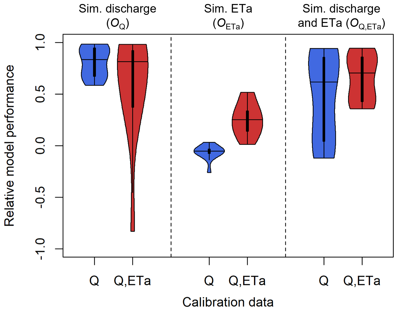
Figure 2 Model performance for simulated discharge (O_Q), actual evapotranspiration (O_ETa), and discharge and actual evapotranspiration (O_Q,ETa) when using discharge (Q; blue boxes), or both discharge and actual evapotranspiration (Q, ETa; red boxes) as calibration data. The figure shows the median of the 100 best performing parameter values of each catchment. To present results for all twelve study catchments, performance values were normalized by an upper benchmark (equal to 1) and a lower benchmark (equal to the median performance of the uncalibrated model). A value of zero means that model performance after calibration is equal to the model performance of the lower benchmark.

By exploring flux maps and hydrograph uncertainties, however, we get a more nuanced and different view of the effect of multivariate calibration on model realism. Figure 3a shows the flux map after different calibration cases for the Litchfield catchment. While interflow and baseflow were the main streamflow generation mechanisms when calibrating to discharge (O_Q), overland flow gained importance when also considering actual evapotranspiration in calibration (O_Q,ETa). Consequently, the percentage of the flux map area filled by the 100 best simulations increased from 14 % after a discharge-only calibration to 41 % when adding actual evapotranspiration to a discharge-based calibration. Such an increase in flux map area was observed for ten out of twelve catchments with flux map areas increasing between 2 % and 27 % (Fig. 3b). This suggests that multivariate calibration can increase simulated flux equifinality regardless of local conditions such as climate type. An interesting exception from this general observation is the Cow Bay catchment. Its flux map area changed by −22 % leading to a more constrained map after multivariate calibration. However, this more constrained flux map is not a subset of the flux map of a discharge-based calibration as one would expect.

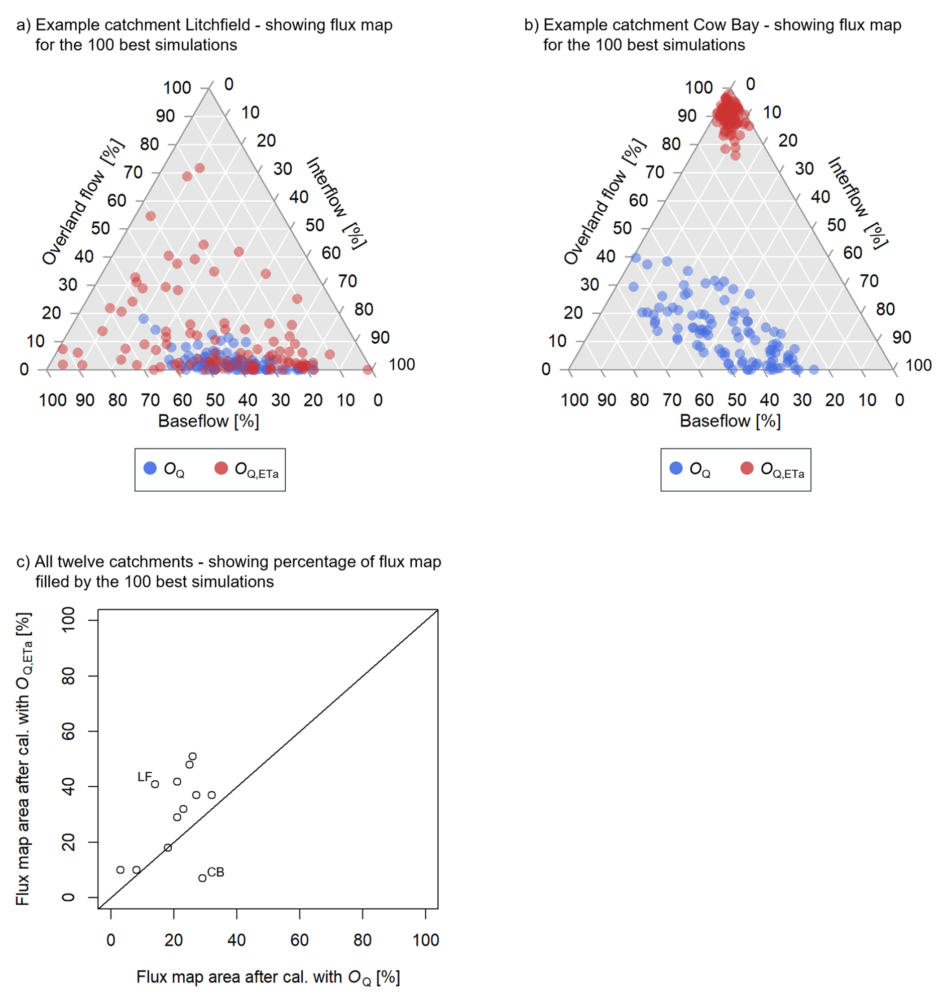
Figure 3 Flux map when calibrating the model with discharge (O_Q) or discharge and actual evapotranspiration (O_Q,ETa). (a, b) The flux map is shown for the 100 best parameter sets in terms of O_Q and O_Q,ETa for the Litchfield (LF) and Cow Bay (CB) catchments. (c) Percentage of flux map area filled by the ensemble of 100 best parameter sets in terms of O_Q and O_Q,ETa. Values are shown for all twelve study catchments.

In terms of hydrograph uncertainty we found that the simulated hydrograph uncertainty of the Litchfield catchment considerably increased for many flow conditions when not only calibrating to discharge (O_Q) but also considering actual evapotranspiration in calibration (O_Q,ETa; Fig. 4a). This observation was common to all study catchments, whereby the increase in hydrograph uncertainty generally tended to be larger for low flows than high flows (Fig. 4b). Averaging over all flow conditions (i.e., simulated time steps), uncertainty increased in eleven out of twelve catchments. The only catchment experiencing a lower average hydrograph uncertainty after multivariate model calibration was Cow Bay. Interestingly, Cow Bay was also the only catchment with a much-reduced flux equifinality when adding actual evapotranspiration to a discharge-based calibration (Fig. 3b and c).

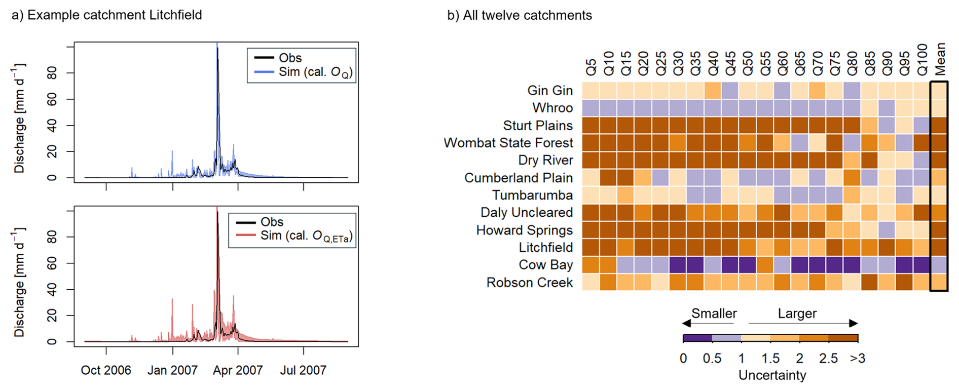
Figure 4 Hydrograph uncertainty when calibrating the model with discharge (O_Q) or discharge and actual evapotranspiration (O_Q,ETa). (a) Observed and simulated hydrograph for the Litchfield catchment in a year with close to mean annual discharge. The range in hydrograph simulations indicates the minimum and maximum value of all 100 best simulations in terms of O_Q and O_Q,ETa. (b) Change in uncertainty of the simulated hydrographs at different flow quantiles (Q5 (low flow) to Q100 (high flows)). Change is defined as the ratio of the simulated range from a calibration with O_Q,ETa to the simulated range from a calibration with O_Q. Values smaller than 1 (purple color) indicate a reduction in uncertainty when adding actual evapotranspiration to a discharge-based calibration. Values are shown for all twelve study catchments.

3.2 Comparing results from univariate calibration with discharge and actual evapotranspiration

To explore why multivariate model calibration increased flux map area and hydrograph uncertainty, we first analysed the model parameter space after calibration. As mentioned previously, Monte Carlo-based multivariable calibration is a way of making an initially large parameter space smaller, whereby the goal is to seek the intersection between the separate behavioural clouds of two or more variables (here, discharge and actual evapotranspiration). It is therefore assumed that such an intersection exists. Here, we looked for these intersections between two clouds by comparing the parameter value distribution when calibrating SIMHYD solely to discharge and solely to actual evapotranspiration. Given SIMHYD has seven parameters, it is possible to assess the intersection of clouds in any number of dimensions between one (i.e., assessing overlap of histograms for each parameter individually) and seven (which is difficult to visualize but technically possible). Here, we focus on two-dimensional plots since they allow some consideration of parameter interactions but are still easy to visualize. We examined parameter distributions for all 21 parameter pairs (unique combinations of seven model parameters). For each catchment, we present the result for one parameter pair as a scatterplot (Fig. 5). The (subjectively) selected examples show different patterns of the lack of overlap (if any) between the separate clouds. Quantitative results for all 21 pairwise parameter combinations can be viewed in Fig. 6 showing the overlap of the convex hull of the behavioural parameter clouds of discharge and evapotranspiration.

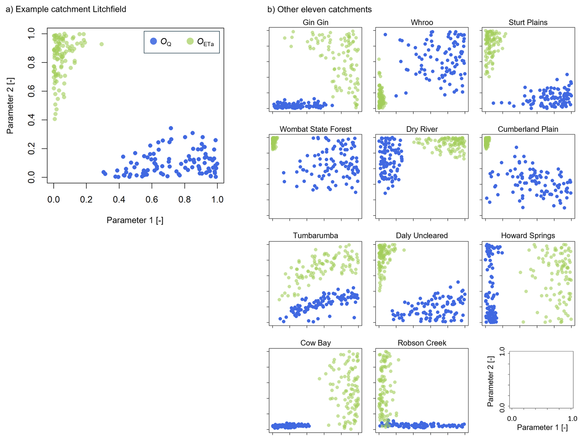
Figure 5 Parameter distribution when calibrating the model with discharge (O_Q) or actual evapotranspiration (O_ETa). (a) Distribution of two parameters for the 100 best parameter sets in terms of O_Q and O_ETa for the Litchfield catchment. In this example, parameter 1 is infiltration loss exponent [–] and parameter 2 is maximum infiltration loss [mm d⁻¹]. (b) Same as in (a) but with an example for the other eleven catchments. Note that all parameter values are normalized [0,1], and parameter 1 and parameter 2 represent different SIMHYD parameters in each case. Parameter combinations were chosen to show different separation patterns. Robson Creek is the only catchment without a point cloud separation in a two-dimensional parameter space when calibrating with O_Q and O_ETa.

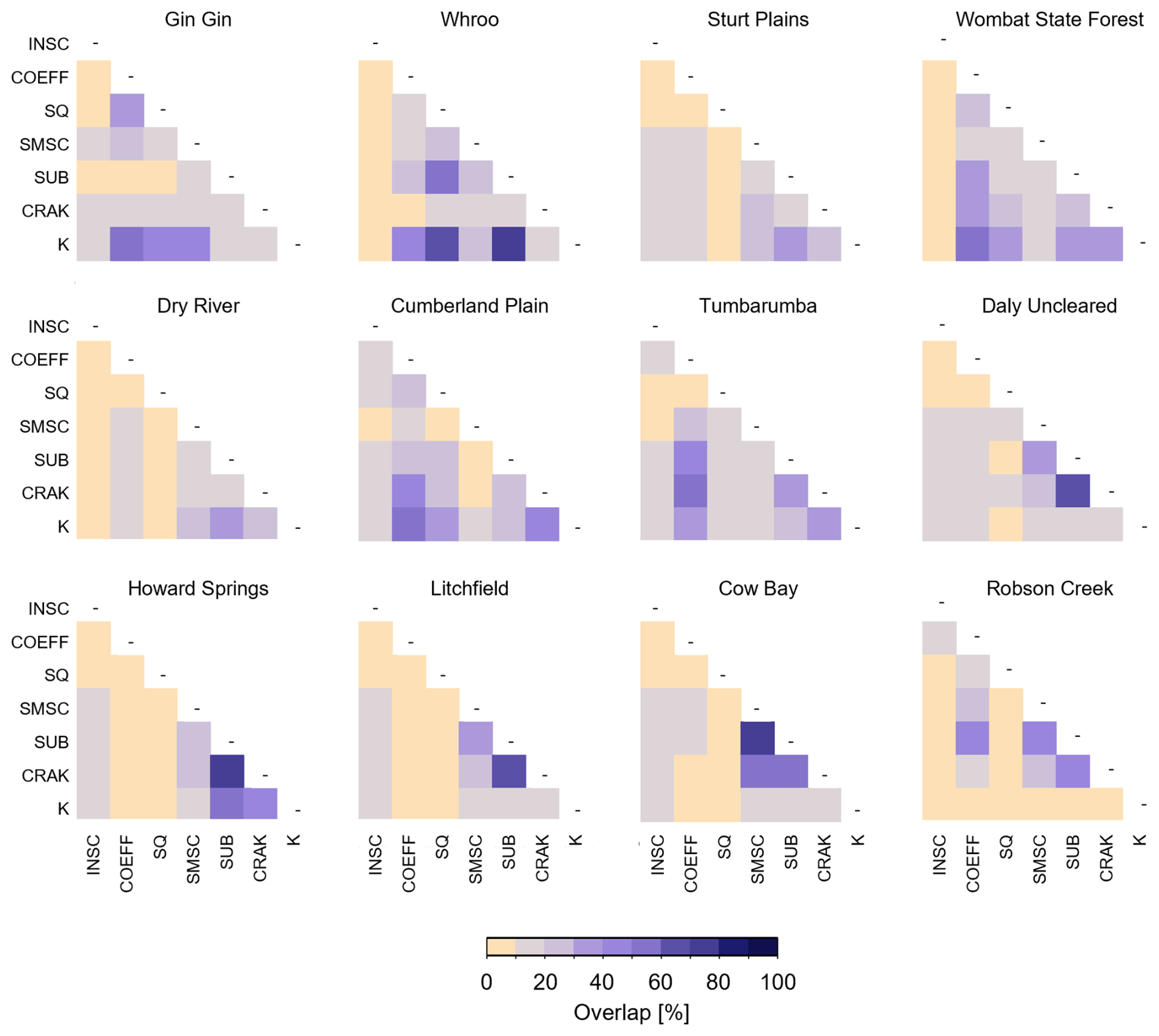
Figure 6 Overlap of the two point clouds of behavioural parameter sets for a given parameter pair when calibrating the model solely to discharge (O_Q) and solely to actual evapotranspiration (O_ETa). The orange squares show the parameter combinations with a lack of overlap in the two-dimensional space. Values range from 0 %–100 % of the total area of the normalized parameter space (as visualized in Fig. 5).

Starting again with the Litchfield catchment as an example, Fig. 5a shows the values of the 100 best parameter sets for two model parameters, namely infiltration loss exponent (x axis) and maximum infiltration loss (y axis), when calibrating SIMHYD with discharge (O_Q) and with actual evapotranspiration (O_ETa). We found that there was a strong separation between the two point clouds of behavioural parameter sets for the given parameter pair and no evidence of intersection as often assumed. Similar results, although with different separation patterns and different parameter pairs, were observed for the other study catchments (Fig. 5b). We expect that the separation patterns would get even more pronounced when moving from the two-dimensional parameter space to a higher dimensional space, but having demonstrated non-overlap in two dimensions for most catchments, we did not explicitly test this in higher dimensions, save by exception. An example of that is the Robson Creek catchment for which the point clouds of behavioural parameter sets overlapped in the two-dimensional parameter space (Fig. 5b) but became separated when analysed in the three-dimensional parameter space (not shown here). While we focused on presenting one example of separation pattern for each catchment, the patterns were typically present for several parameter pairs.

We further analysed how a calibration with discharge and a calibration with actual evapotranspiration affected the simulated contribution of streamflow generation mechanisms. In the case of the Litchfield catchment (Fig. 7a), a calibration with discharge (O_Q) favoured parameter sets for which streamflow was largely composed of interflow and baseflow. In contrast, much of the total streamflow originated from overland flow when calibrating solely to actual evapotranspiration (O_ETa). Such considerable discrepancies in streamflow generation mechanisms were also observed for other study catchments (Fig. 7b). They could eventually lead to a larger flux map equifinality when simultaneously calibrating to discharge and actual evapotranspiration, which was indeed observed in Fig. 3.

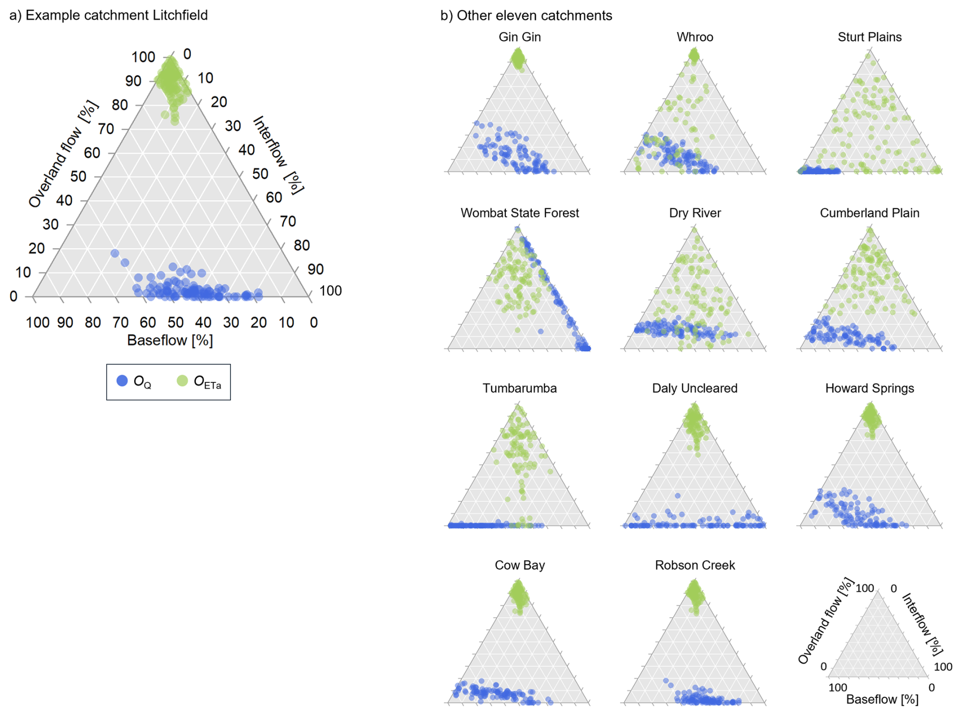
Figure 7 Flux map when calibrating the model with discharge (O_Q) or actual evapotranspiration (O_ETa). (a) The flux map is shown for the 100 best parameter sets in terms of O_Q and O_ETa for the Litchfield catchment. (b) Same as in (a) but for the other eleven catchments.

4 Discussion

4.1 Why did multivariate calibration increase discharge uncertainty?

Our results for twelve hydrologically contrasting catchments in Australia suggest that multivariate model calibration can lead to less constrained flux maps (i.e., streamflow generation mechanisms) and consequently increased hydrograph uncertainties relative to a discharge-based calibration (Figs. 3 and 4). These results may seem counterintuitive given the large number of studies reporting improved realism for a range of simulated variables and processes after multivariate calibration (e.g., Demirel et al., 2019; Mei et al., 2023; Meyer Oliveira et al., 2021). Thus, why does the inclusion of additional information not result in more constrained flux maps and hydrographs? The parameter distributions shown in Figs. 5 and 6 suggest that these symptoms could be caused by non-overlapping behavioural parameter distributions for the individual calibration variables. When simultaneously calibrating the model against discharge and actual evapotranspiration, overall model performance (i.e., the average performance over both variables) increases (by definition, since this is the objective function used). However, in the absence of an intersection between the individual behavioural clouds, the selected parameter sets represent compromise solutions that get spread across or between the two individual clouds (Figs. S5 and S13 in the Supplement), sometimes covering a wider space, which increases equifinality and finally leads to increased discharge uncertainty.

Under ideal conditions, there would, for each catchment, be one single parameter set resulting in a perfect match between several observed and simulated variables. However, the process of setting up a model for a catchment involves a large number of (subjective) decisions, including the choice of data, calibration procedure, and model structure, which all affect the study outcome (Ceola et al., 2015). Below we discuss some aspects of these decisions, which we think are relevant in the context of our work.

We used actual evapotranspiration data from two different sources. Field-based actual evapotranspiration data from flux towers are considered to be more accurate than remote sensing-based data and are used to benchmark the latter (Martens et al., 2017; Zhang et al., 2010). The near-point-scale nature of flux tower data means they are not necessarily representative of the entire (sub-) catchment, a fact known to affect the suitability of local observations to select catchment-scale parameter values (Gallart et al., 2007; Staudinger et al., 2021; Széles et al., 2020). Remote sensing-based actual evapotranspiration data may have a larger footprint and while many data products show reasonable seasonal dynamics, they can suffer from large volume bias (Elnashar et al., 2021; Wartenburger et al., 2018; Zhang et al., 2020). The choice of an evapotranspiration data product can significantly influence the selection of model parameter values even if a bias insensitive metric was used in calibration (Dembélé et al., 2020b; Nijzink et al., 2018). Interestingly, the remote sensing-based data and the field-based flux tower data led to similar observations for the twelve study catchments despite their different data characteristics: non-overlapping behavioural parameter distributions were present for both datasets, flux map patterns were similar for the individual calibration variables, and the direction of the correlation between the two calibration variables in a given catchment tended to be the same in both datasets. We take this as an indication that issues with actual evapotranspiration data are not the root cause of the results. Thus, changing the actual evapotranspiration datasets would be unlikely to result in significantly different conclusions. While gauging errors in discharge data influence results, these errors might be expected to differ from one station to the next, whereas the issues here occur across all twelve catchments tested. Thus, it appears data quality alone cannot explain the increased discharge uncertainty following multivariate calibration.

Another potential factor influencing our results is the calibration process. For example, the choice of an objective function defines which aspects of a time series receive most weight during calibration (Kiesel et al., 2017; Pool et al., 2017) and thus changes the distribution of the calibrated model parameter values (Choi and Beven, 2007; Garcia et al., 2017). We used objective functions that tend to simultaneously evaluate a range of data aspects as we were interested in a model being able to simulate multiple facets of catchment response. Both objective functions were based on the Kling–Gupta efficiency and represent a choice done in many modelling studies. Another commonly used objective function, the Nash–Sutcliffe efficiency (Nash and Sutcliffe, 1970), is in many aspects similar to KGE and its use should result in similar findings as made in this study. When conducting the multivariate calibration, we combined the individual objective functions for discharge and actual evapotranspiration into a single combined objective function (Eq. 3) as opposed to the simultaneous evaluation of two separate objective functions. This approach has the drawback that the selection of behavioural parameter sets can get biased towards one of the two calibration variables and increase the uncertainty of the other simulated variable, especially if pronounced trade-offs exist. While trade-offs have been reported in many previous studies irrespective of the multivariate calibration approach (Livneh and Lettenmaier, 2012; Mostafaie et al., 2018; Yassin et al., 2017), they were rarely shown to increase discharge uncertainty. We discuss this in more detail in Sect. 4.2.

A probably more impactful factor in our study was the decision to define the 0.1 % best performing parameter sets as behavioural. Loosening this threshold may increase the chance of finding overlapping parameter distributions for univariate calibrations with discharge and actual evapotranspiration. This would come at the expense of accepting lower model performance values for the calibration variables although the extent of these costs differs among catchments and the threshold (Fig. 8a). The choice of a threshold also affects how much parameter values are constrained. Results for the parameter values are more consistent among catchments than for model performance and generally indicate that parameter values get quickly less constrained with an increasing number of behavioural parameter sets (Fig. 8b). Most parameters in SIMHYD directly affect runoff generation and a wider range of their values can further increase flux equifinality and thus hydrograph uncertainty. This is similar to findings reported in a study by Lamb et al. (1998), where less constrained TOPMODEL parameter values and wider discharge uncertainty bounds were found for multivariate calibration than in a discharge-based calibration. Thus, working with the best 100 parameter sets seems to be a reasonable decision for this study. However, performance thresholds are only one relevant factor in a broad set of methodological choices that contributed to the result seen here, as discussed below in more detail in Sect. 4.2.

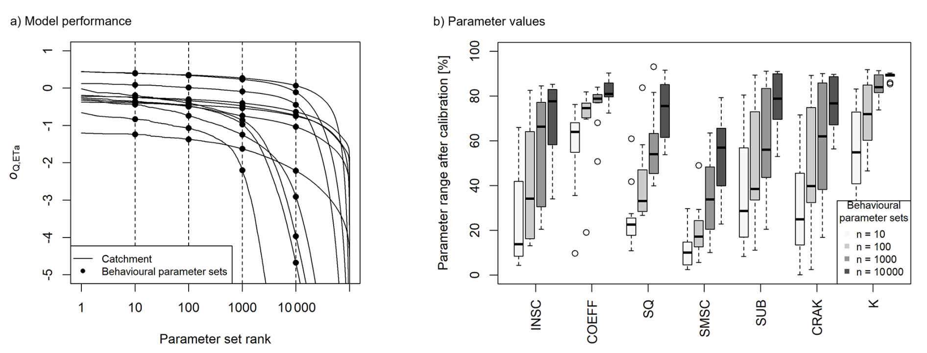
Figure 8 Definition of behavioural parameter sets and its impact on (a) model performance O_Q,ETa and (b) parameter values, i.e., ratio of the range of parameter values after calibration with O_Q,ETa relative to the range of possible parameter values before calibration (see Fig. S1 for an explanation of the parameters). Results are shown for all twelve study catchments.

4.2 Methodological choices contributing to the study result

Although unplanned, the combination of two key methodological decisions led directly to the observed result being possible. Had either decision been made differently, the non-overlap of the individual parameter clouds (Figs. 5 and 6) would have presented with different symptoms. The two key methodological decisions are explained in Fig. 9. The first decision was whether to require parameter sets to fulfil acceptance criteria for both variables separately (horizontal axis in Fig. 9), which we did not do. Instead, acceptance was assessed based on average performance across variables. Had this decision gone the other way, no parameter set in the top 100 for discharge would have also been in the top 100 for actual evapotranspiration, and vice versa. In this case, the symptom of non-overlapping clouds would be that no behavioural parameter sets would be found. The second decision was whether to require a pre-defined performance threshold to be met (vertical axis in Fig. 9), which we did not do. Instead, the top 100 parameter sets were accepted, whatever their performance may be. Had this decision gone the other way, it is unlikely that any parameter set would have met the threshold because, at best, they might be located in one behavioural cloud but not the other, and never both. Thus, they would all have a poor average score across the two variables, and (once again) the symptom of non-overlapping clouds would be that no behavioural parameter sets would be found. Consequently, all methodological options except the one adopted would lead to no behavioural sets and make the observed result impossible. It is, however, important to note that (i) we are not advocating one of these methods over the others, but rather reflecting on the circumstances that gave rise to the results; and (ii) the issue of non-overlapping parameter clouds is present irrespective of the chosen calibration approach or whether the non-overlap is detected during calibration or not.

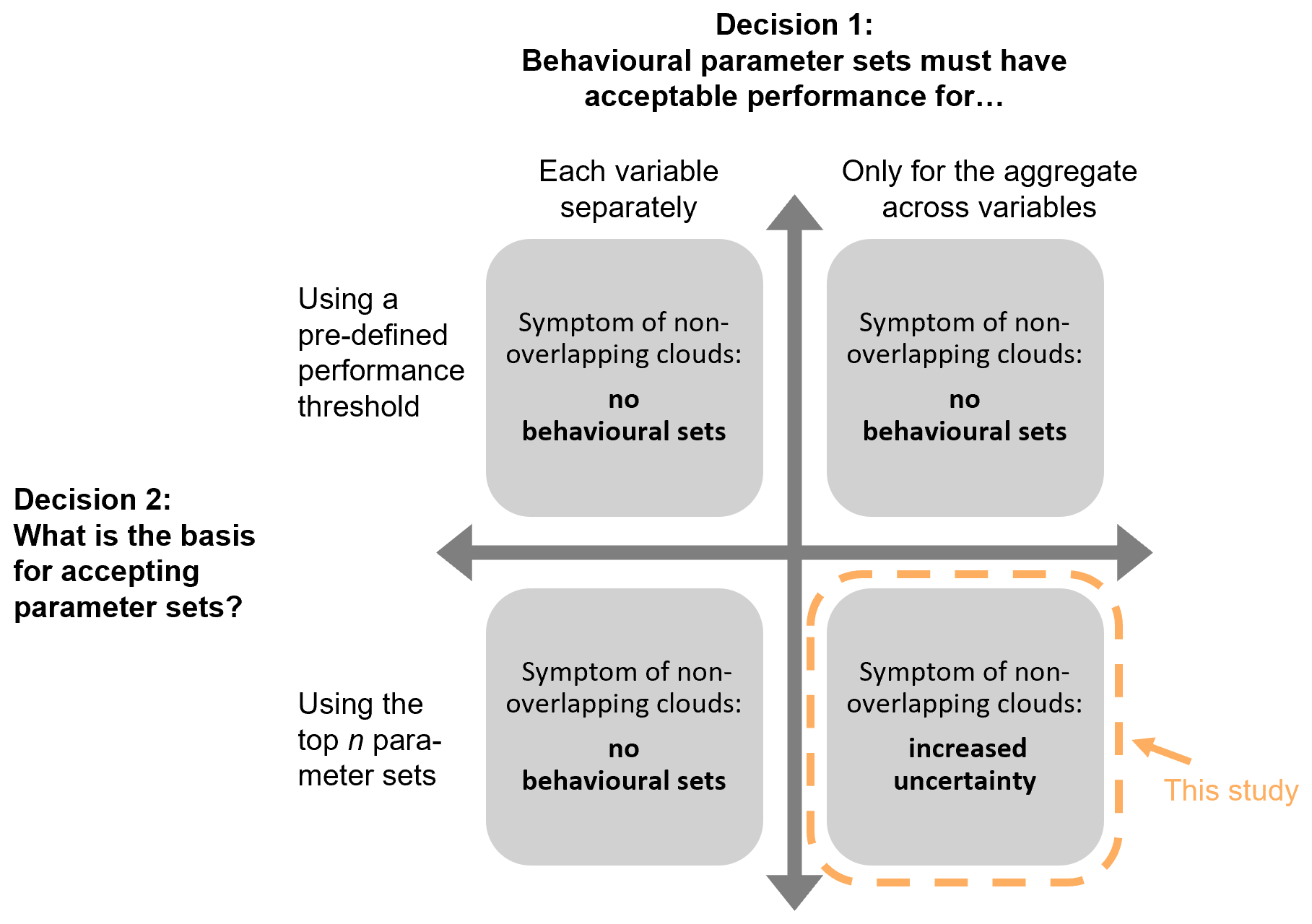
Figure 9 Matrix of possible design choices for this modelling experiment, showing the distinct combination that made the observed result possible.

It is possible that many prior studies have also come across the problem of non-overlapping clouds using one of the other three methods outlined above, and thus they identified no behavioural parameter sets. This null result is sufficient to scuttle a study before it has even begun, and so it is likely that those authors altered the parameters of their study until a workaround was found. If this is true, it would explain why few papers have reported similar findings. However, we recommend that future studies recognise such problems, report them, and attempt to tackle them directly rather than seeking workarounds that leave the core problem unresolved and unreported. This is particularly important in the case of model structural inadequacy, whereby we need greater insights to distinguish among candidate models and provide evidence-based reasons to move away from legacy-based model selection (Addor and Melsen, 2019). These ideas are expanded further in the following sections.

4.3 Increased uncertainty as a sign of model structural inadequacy

Differences in parameter distributions or trade-offs in model performance when using multiple calibration variables can be a sign of model structural limitations. For example, Meyer Oliveira et al. (2021) found contrasting soil water storage capacity values after calibrating the MGB model with discharge or actual evapotranspiration for the Amazonas. They attributed the large differences to parameter compensation effects caused by a misrepresentation of processes related to deep root water uptake during the dry season. Vervoort et al. (2014) modelled four Australian sub-catchments with the CMD model and showed that adding actual evapotranspiration to a discharge-based calibration improved the simulated water balance, but negatively affected the timing of discharge simulations. They argued that multivariate calibration left less room for the parameters to compensate for structural errors in the conceptualization of potential flow paths. In the context of a discharge-only calibration but using multiple seasons and performance criteria, Choi and Beven (2007) also found that no TOPMODEL parameter sets were behavioural over all conditions defined for the Bukmoon catchment (South Korea). Their results suggest that adapting the model to allow for the seasonally changing recession and evapotranspiration characteristics may be needed to improve discharge simulations. In our work, the non-overlapping (but often rather well constrained) parameter distributions and contrasting flux maps suggest very different hydrological responses for the same catchment when calibrating with discharge or actual evapotranspiration. A common observation among many catchments was that a calibration with actual evapotranspiration resulted in a large fraction of (infiltration excess) overland flow, whereas a calibration with discharge resulted in a combination of interflow and baseflow. Such a contrasting behaviour could potentially be caused by limitations in the conceptualization of the soil store. However, to better identify and understand structural limitations of the SIMHYD model, a much more comprehensive analysis targeted to detect limitations would be needed.

4.4 Multivariate model calibration – an insightful test for evaluating hydrological models

Given the wide range of available models and their application for diverse purposes, it is desirable to apply tests to identify their suitability, and we believe the multivariate methods shown here could inform such a model testing. Some of the most widely applied model testing frameworks are based on the four-level testing scheme proposed by Klemeš (1986) in which the model's transposability is tested in time and space. Various variants of the split sample test (SST), such as the generalized SST (GSST; Coron et al., 2012) or a generalized differential SST (GDSST; Dakhlaoui et al., 2017), have been developed to thoroughly test the temporal robustness of models under changing conditions. There is also a long history of large sample catchment studies, which were conducted to better understand the applicability of a model across hydrologically contrasting catchments (Knoben et al., 2020; Merz and Blöschl, 2004; Perrin et al., 2001; Seibert et al., 2018). These tests are typically conducted using locally observed discharge data although they are applicable to any type and number of hydrological data. For example, one can test a model by calibrating it with one variable (e.g., discharge) and evaluating it with withheld data (e.g., actual evapotranspiration), as done in this study. Thus, the calibration and evaluation with multiple hydrological variables can be seen as an additional dimension of the tests proposed by Klemeš (1986).

Interestingly, the benefits of multivariate calibration are rarely evaluated in the context of testing (as outlined above) and potentially rejecting a model structure. Multivariate calibration studies are more often motivated by the specific need for discharge simulations in ungauged basins (Hulsman et al., 2020; Liu et al., 2022; Zhang et al., 2020) or the more general interest in improving model realism within the limits of a chosen model structure (Demirel et al., 2019; Finger et al., 2015; Széles et al., 2020). Our work suggests that the value of multivariate model calibration goes beyond estimating parameter values, and we think multivariate calibration can serve as an insightful test of a model's capacity to represent hydrological behaviour, especially if a range of modelled aspects are considered. Indeed, by evaluating model performance values, we would have concluded that multivariate calibration improves the overall realism of the SIMHYD model (Figs. 2 and S2). However, the flux maps and the parameter distributions (Figs. 5–7) provided important insights into model structural issues and perverse outcomes such as some adopted parameter sets being “compromise” solutions in subregions not associated with either variable's behavioural subspace.

Our results were based on a few catchments in Australia and a single model structure. Yet, the chosen modelling set-up allowed us to test and falsify the two, often implicitly assumed, hypotheses motivating this study. As discussed by the philosopher Karl Popper (Popper, 2002), the observation of a single example contradicting a hypothesis is sufficient to reject it. To additionally evaluate the generalizability of our findings, we encourage modellers to further explore the potential of multivariate model calibration for testing models on a larger catchment data set, a wider set of different models, and other types of data. Open-source model collections like MARRMoT (Trotter et al., 2022) facilitate the testing and comparison of several existing model structures. Data to set-up, run, and evaluate hydrological models for many catchments across the world have also become easily accessible in recent years through the publication of data sets such as CAMELS (Addor et al., 2017; Alvarez-Garreton et al., 2018; Coxon et al., 2020; Fowler et al., 2024). The preparation of remote sensing-based hydrological variables other than discharge for hydrological modelling is still more tedious, but modelers can often choose between several publicly available products for a particular variable (Awasthi and Varade, 2021; Beck et al., 2021; Elnashar et al., 2021). A major challenge though is access to data quality information, especially in the context of large-sample hydrology. The consideration of potential errors in data, for example by a limits of acceptability approach (Freer et al., 2004), can ideally form part of a thorough model testing scheme.

The more recent combined availability of models and data provides a great opportunity to evaluate the appropriateness and limitations of a particular model structure or its parameter values. While we used discharge and actual evapotranspiration to select behavioural parameter sets in a Monte Carlo-based approach, a similar concept can be applied with any variable of interest. In fact, a detailed model testing with multivariate calibration will be most insightful if conducted for variables most relevant for a particular scientific or operational purpose, such as the use of groundwater or terrestrial water storage in catchments showing multi-year “memory” (Fowler et al., 2020) or the need to match vegetation dynamics that might be driving catchment behaviour (Gardiya Weligamage et al., 2023; Peterson et al., 2021). As discussed by Andréassian et al. (2009), we need to be merciless towards our own models by applying demanding crash-tests. Calibrating with multiple variables, aside from being motivated by model realism, can be a powerful additional crash test for our models.

5 Conclusions

The main goal of this study was to assess the impact of multivariate model calibration on uncertainty in simulated flux maps (i.e., streamflow generation mechanism) and hydrographs. We used a Monte Carlo-based approach in which an initially large sample of 100 000 parameter sets was constrained using discharge only, actual evapotranspiration only, and a combination of both variables. For each of these three calibration cases, the 100 best parameter sets were retained and the related parameter distributions, flux maps, and hydrographs were analysed. Our modelling experiment was based on twelve Australian catchments covering a range of hydroclimatic conditions.

We found that calibration with both discharge and actual evapotranspiration rather than discharge only led to a less constrained flux map and thus a wider range of potential streamflow generation mechanisms for a given catchment. This eventuated in increased hydrograph uncertainty for many different flow conditions and for 11 of 12 study catchments. Our results suggest that these symptoms could be caused by non-overlapping behavioural parameter distributions (or parameter clouds when visualized in the two-dimensional parameter space) following a calibration with the individual variables. Thus, when simultaneously calibrating the model against discharge and actual evapotranspiration, the selected behavioural parameter sets represented compromise solutions that were often part of neither behavioural cloud and that were spread widely through the parameter space, which increased flux equifinality and discharge uncertainty. While there can be various reasons why behavioural parameter distributions from different calibration variables don't overlap, in our study context, they likely point towards model structural limitations. The observation of non-overlapping behavioural parameter clouds has rarely been reported in the literature and may contradict the expectations commonly found within the hydrological modelling community. We recommend that future studies recognise such problems and report them to contribute to an improved understanding of the value of data for model calibration and selection.

Our findings can contribute to good modelling practices in two ways. First, multivariate calibration is an important tool for selecting more realistic model parameter values. However, our results suggest that model realism should not purely be assessed with a performance criterion. Instead, we recommend to carefully analyse the distribution of behavioural parameter values for each calibration variable and to test the assumption of overlapping behavioural parameter clouds before drawing conclusions on model realism. Second, non-overlapping behavioural parameter clouds suggest that the value of non-discharge data for model calibration is contingent on the suitability of the model structure. By evaluating the overlap in the parameter space, multivariate model evaluation can be a powerful way to test a model structure and thus support the decision to either accept or reject it. We recommend research to develop such ideas for model rejection further.