Introducing the Model Fidelity Metric (MFM) for robust and diagnostic land surface model evaluation

The accurate evaluation of Land Surface Models (LSMs) is fundamental to their development and application. However, baseline metrics such as the Nash-Sutcliffe Efficiency (NSE) and Kling-Gupta Efficiency (KGE) possess well-documented shortcomings in inappropriate contexts. Relying on moment-based statistics such as mean, variance, and correlation often falls short for land surface modelling data, which are typically non-normal and skewed. These metrics can be misleading due to issues such as error compensation, instability when variability is low, and the confusion of magnitude and phase errors, leading to inaccurate model assessments. To provide a reliable overall score, we propose the Model Fidelity Metric (MFM), a novel evaluation framework constructed using robust statistics and information theory. MFM integrates three orthogonal dimensions of model performance within a Euclidean framework, including (1) Accuracy, which is measured by the robust Normalized Mean Absolute p-Error (NMAEp) and penalized for timing issues via a Phase Penalty Factor (PPF); (2) Variability, quantified using the information-theoretic Scaled and Unscaled Shannon Entropy differences (SUSE); and (3) Distribution similarity, assessed non-parametrically using the Percentage of Histogram Intersection (PHI). We evaluated MFM against traditional metrics using targeted synthetic experiments and the large-sample CAMELS dataset. Our results demonstrate that MFM provides a more authentic and reliable assessment of model fidelity. MFM proved to mitigate error compensation effects that mislead KGE and remained stable in low-variability scenarios where NSE and KGE fail. Furthermore, MFM provides superior diagnostic capabilities by decoupling phase and magnitude errors and decomposing performance into its core components. This work highlights the need to move beyond traditional moment-based metrics. We advocate adopting robust, diagnostic frameworks such as MFM to support the development of more trustworthy LSMs.

1 Introduction

Land Surface Model (LSM) performance metrics serve as the foundation for model evaluation, calibration, parameter optimisation, and intercomparison studies (Clark et al., 2021; Gupta et al., 2009). LSMs produce outputs such as latent heat flux, soil moisture, and runoff. They form the core of the Earth System Models (ESMs) and Numerical Weather Prediction (NWP) systems (Dai et al., 2003). Accurate modelling is critical for climate projection, extreme event forecasting, and water resource management (Best et al., 2011). By condensing the complex, high-dimensional relationship between observed and simulated time series into a single numerical score, these metrics enable objective model assessment and facilitate decision-making in water resources management, flood forecasting, and climate impact studies (Mizukami et al., 2019). The choice of performance metric highly affects model development trajectories, shapes our understanding of land surface processes, and ultimately determines the reliability of model-based predictions (Cinkus et al., 2023).

The evolution of LSM metrics began with simple error measures like the Root Mean Square Error (RMSE), which calculates the Euclidean distance between simulations (S) and observations (O):

$$\begin{array}{}\text{(1)}& \mathrm{RMSE}=\sqrt{{\displaystyle \frac{\sum (S_i-O_i{)}^{\mathrm{2}}}{n}}}.\end{array}$$

Subscript i denotes the ith time step, n is the length of the time series.

Recognizing the limitations of scale-dependence of RMSE, Nash and Sutcliffe (1970) introduced the Nash-Sutcliffe Efficiency (NSE), which is widely used for LSM evaluation:

$$\begin{array}{}\text{(2)}& \mathrm{NSE}=\mathrm{1}-{\displaystyle \frac{(\mathrm{RMSE}{)}^{\mathrm{2}}}{{\mathit{\sigma }}_O^{\mathrm{2}}}},\end{array}$$

where σ_O is the standard deviation of observations (Nash and Sutcliffe, 1970). NSE provides a dimensionless indicator of model skill relative to a mean benchmark. The quadratic form makes it highly sensitive to outliers and thus well suited for streamflow evaluation with a focus on peak flow. However, the inappropriate application of NSE can lead to erroneous conclusions (Gupta et al., 2009; Legates and McCabe, 1999).

To address these shortcomings, Gupta et al. (2009) proposed the Kling-Gupta efficiency (KGE). KGE provides a more balanced assessment by decomposing performance into three distinct components within a Euclidean distance from their ideal values:

$$\begin{array}{}\text{(3)}& \begin{array}{rl}\mathrm{KGE}& =\mathrm{1}-\sqrt{(r-\mathrm{1}{)}^{\mathrm{2}}+({\displaystyle \frac{{\mathit{\sigma }}_S}{{\mathit{\sigma }}_O}}-\mathrm{1}{)}^{\mathrm{2}}+({\displaystyle \frac{{\mathit{\mu }}_S}{{\mathit{\mu }}_O}}-\mathrm{1}{)}^{\mathrm{2}}}\\ & =\mathrm{1}-\sqrt{(r-\mathrm{1}{)}^{\mathrm{2}}+(\mathit{\alpha }-\mathrm{1}{)}^{\mathrm{2}}+(\mathit{\beta }-\mathrm{1}{)}^{\mathrm{2}}},\end{array}\end{array}$$

where r is the Pearson correlation coefficient, α is the relative variability, β is the bias ratio. Together, NSE and KGE now dominate the land surface modelling literature, serving as the primary criteria for model calibration and performance assessment across diverse applications and geographical regions (Knoben et al., 2019; Pool et al., 2018). Their widespread adoption has established them as a universal method for assessing model performance, as evidenced by numerous studies, operational systems, and extensive model comparison initiatives such as the Coupled Model Intercomparison Project Phase 6 (CMIP6; Eyring et al., 2016).

However, recent research has increasingly highlighted that the inappropriate application of the NSE and KGE frameworks challenges their reliability as comprehensive indicators of model fidelity (Cinkus et al., 2023; Clark et al., 2021; Schaefli and Gupta, 2007). A critical vulnerability of KGE is its susceptibility to error compensation, in which opposing errors across different parts of time series cancel each other out, yielding misleadingly favourable scores. Although the Pearson correlation coefficient r can help penalize this issue, relative variability α and bias ratio β can cause the KGE to assign higher scores to objectively more biased models. Cinkus et al. (2023) demonstrated this phenomenon through systematic synthetic experiments, showing that KGE can assign higher scores to models that simultaneously overestimate and underestimate discharge compared to models with consistent but unidirectional errors. This behaviour occurs since KGE's variability parameter (α) and bias parameter (β) are based on moment-based statistics (mean and standard deviation, see Eq. 3). These statistics are most effective for normally distributed data (Fig. S1 in the Supplement). However, when applied to non-normal, heavy-tailed, and skewed distributions common in land surface modelling data, these statistics are highly sensitive to outliers and do not accurately reflect the true characteristics of the system (Fu and Zhang, 2024; Mizukami et al., 2019). Since these two components typically account for two-thirds of the weight in KGE formulations, error compensation effects can dominate the overall score, rewarding models for being “right for the wrong reasons”. For example, Cinkus et al. (2023) showed the bias ratio and variability scores were 11 % and 13 % respectively higher for the worse model. This occurs because the errors in worse model happen to cancel each other out, not because the model is genuinely better than models with lower KGE. Meanwhile, Cinkus et al. (2023) also tested 130 321 synthetic hydrographs subjected to controlled transformations to assess their impact across nine performance metrics. They discovered that the standard KGE and its variants (mKGE, KGE', KGE”) were all highly responsive to these balancing errors. Their analysis showed that models with lower actual skill often scored higher on KGE because of coincidental error cancellation. This fundamental problem questions KGE's validity as a full performance measure and casts doubt on studies that mainly depend on KGE-based evaluations. These limitations, including error compensation, instability under low-variability conditions, sensitivity to outliers in non-normal and highly skewed distributions, and failure to reflect the true characteristics of the system, are not merely theoretical concerns but also lead to systematic biases in model selection, misleading performance rankings, and potentially incorrect conclusions about model skill across different land surface modelling regimes (Klotz et al., 2024; Knoben et al., 2025).

Lamontagne et al. (2020) and Clark et al. (2021) emphasized a significant vulnerability, namely the high sampling uncertainty in NSE and KGE, which is caused by the heavy-tailed distribution of squared errors. Analysis of 671 catchments from the Catchment Attributes and Meteorology for Large-sample Studies (CAMELS) dataset showed that performance metric scores are significantly affected by a limited number of extreme data points, with fewer than 0.5 % of simulation-observation pairs accounting for 50 % of the sum-of-squared errors (Clark et al., 2021). This high sensitivity to outliers leads to considerable sampling variability, with 90 % tolerance intervals for NSE and KGE exceeding 0.1 in more than half of the catchments examined, suggesting that performance differences below this threshold may be statistically insignificant. The sampling uncertainty problem becomes particularly acute in arid regions and during low-flow conditions, where near-zero observed flows in the denominator render NSE and KGE numerically unstable (Santos et al., 2018). Under these conditions, a single outlier can cause the metric to shift from near ideal to very negative, making these metrics unreliable for comparing models. This instability suggests practical implications for model choice and water management, especially in water-scarce areas where precise low-flow predictions are vital (Pool et al., 2018).

Similar issue occurs for NSE metrics. Despite NSE's squared-error formulation, which theoretically emphasizes large errors, Mizukami et al. (2019) found that NSE-based calibration systematically underestimates annual peak flows by more than 20 % at median values across 492 hydrologically unregulated catchments in the contiguous United States. This interesting finding arises because NSE tends to underestimate observed flow variability. While KGE partially addresses this issue by explicitly including a variability ratio term (α), both metrics struggle to represent model accuracy, which is critical for flooding risk assessment (Williams, 2025).

Nevertheless, the Pearson's correlation coefficient (r), which assumes linear relationships and is designed for normally distributed data, also limits the application of NSE and KGE. Hydrological time series, especially daily streamflow, often show highly skewed, non-normal distributions with high coefficients of variation (Bhatti et al., 2019). For such data, Pearson's r is severely upward-biased and highly variable, making it an unreliable measure of model-observation agreement. Barber et al. (2020) demonstrated this issue across 905 calibrated rainfall-runoff models, recommending alternative correlation measures such as Spearman's rank correlation or log-transformed correlation that are more robust to non-normality and outliers. Furthermore, the correlation component in KGE conflates magnitude errors with timing errors, creating a “double penalty” problem (Cinkus et al., 2023; Mathevet et al., 2020; Santos et al., 2018). A simulation that accurately reproduces the magnitude and shape of a hydrograph but is slightly shifted in time will be severely penalized in both the correlation term and the point-wise error metrics. Despite this, it remains structurally sound and potentially useful for many applications such as water resource management where total volume or seasonal trends are more critical than time series accuracy (Liu et al., 2011; Magyar and Sambridge, 2023). This issue becomes particularly problematic when evaluating models with uncertain timing of forcing data. It also affects routing-dominated systems, where even slight temporal misalignment is problematic.

Land surface variables such as soil moisture, latent heat flux, and evapotranspiration exhibit highly skewed non-normal distributions. When applied to non-normal distributions, moment-based statistics can produce misleading artifacts. In a normal distribution, the mean, median, and mode coincide due to symmetry, making the mean a faithful representation of central tendency. In skewed or bimodal distributions, however, these statistics diverge, and condensing the entire distribution into a single summary value entails substantial information loss (Fig. S1). Evaluations based on KGE and NSE, facing the problems mentioned above, may result in biased performance assessments. Therefore, a non-parametric, robust, and diagnostic framework is required to accurately evaluate model fidelity across these variables.

Recognizing the limitations of variance-based statistical measures, LSM researchers have increasingly turned to information theory as an alternative framework for model evaluation. Shannon entropy quantifies the uncertainty or information content of a probability distribution in a nonparametric manner, making it naturally suited to characterizing the highly skewed, non-normal distributions typical of hydrological data (Pechlivanidis et al., 2014). Unlike standard deviation, which is dominated by extreme values and susceptible to error compensation, entropy captures the entire shape of the probability distribution and provides a robust measure of system variability and complexity. Pechlivanidis et al. (2010) proposed the Scaled and Unscaled Shannon Entropy differences (SUSE) measure for hydrological and land surface models evaluation. By computing entropy differences using both common bins (scaled entropy) and individual bins (unscaled entropy), SUSE provides a comprehensive assessment of distributional similarity that is holistic under different distributions. Their multi-objective calibration framework combining SUSE with traditional metrics achieved superior performance compared to single-objective or conventional multi-objective approaches by extracting complementary information from different flow regimes (Pechlivanidis et al., 2014). Most recently, Pizarro et al. (2025) developed the Ratio of Uncertainty to Mutual Information (RUMI) metric, which integrates Shannon entropy with uncertainty quantification from the BLUECAT method (Koutsoyiannis and Montanari, 2022). Testing across 99 Chilean catchments spanning diverse macroclimatic zones, RUMI-based simulations outperformed 82 % of 50 hydrological signatures analyzed, with notably lower variability in both calibration and validation periods. This success highlights the practical benefits of information-theoretic methods. It also integrates confidence intervals directly into the evaluation process, rather than treating them as an afterthought.

Histogram-based comparison methods offer another promising avenue for robust model evaluation. The Percentage of Histogram Intersection (PHI), originally developed for color indexing in computer vision (Swain and Ballard, 1991), measures the overlap between two probability distributions in a nonparametric manner. By comparing entire distributions bin-by-bin rather than relying on summary statistics like means or standard deviations, PHI captures the full statistical signature of model performance without making assumptions about data normality or stationarity. This distribution-matching approach is particularly relevant for LSM evaluation because it naturally handles multimodal distributions, captures extreme-value behaviour, and is invariant to monotonic transformations. Unlike KGE's bias term (β), which reduces the entire distributional comparison to a single ratio of means, PHI assesses whether the model reproduces the complete frequency distribution of observed flows from low flows to extreme peaks. This comprehensive assessment is essential for models intended to support diverse management objectives, from drought planning to flood protection.

A growing body of research emphasizes the importance of distinguishing temporal misalignment from amplitude errors in model evaluation. Liu et al. (2011) demonstrated using wavelet transform analysis that timing errors and magnitude errors often arise from different sources (e.g., routing inaccuracies versus rainfall-runoff process representation) and should therefore be evaluated separately. Their wavelet-based timing adjustment reduced root mean square error (RMSE) from 31.4 to 18.9 m³ s⁻¹ and increased correlation from 0.67 to 0.94 for synthetic examples, showing that traditional metrics severely penalize timing-shifted simulations even when the magnitudes are accurate. More recently, the Wasserstein distance (Magyar and Sambridge, 2023), a metric derived from optimal transport theory, was introduced as a LSM objective function that inherently accommodates timing errors by comparing mass distributions rather than point-wise differences. Wasserstein distance addresses the “double penalty” problem by measuring the minimum effort required to transform one distribution into another, accounting for spatial and temporal displacement of features. While computationally more intensive than traditional metrics, Wasserstein distance provides superior performance when displacement errors are present, a common situation in land surface modelling due to uncertainties in rainfall timing and routing processes.

In summary, the evidence presented above reveals a clear need for performance metrics that (1) mitigate error compensation effects, (2) remain stable and reliable in low-variability conditions, (3) robustly address non-normal, heavy-tailed distributions typical of LSM data, (4) separate timing errors from magnitude errors, and (5) offer diagnostically meaningful decomposition to aid model improvement. To address these requirements, we propose the Model Fidelity Metric (MFM), a comprehensive performance criterion built on three orthogonal components grounded in robust statistics and information theory. MFM integrates four fundamental aspects of model performance into these three dimensions, with the detailed definitions provided in Sect. 2:

1. Normalized Mean Absolute p-Error (NMAEp): A flexible, robust measure of overall simulation accuracy based on L_p-norm, which is inherently immune to error compensation. It allows transparent control over sensitivity to outliers through the exponent parameter p without introducing arbitrary component weighting.

2. Scaled and Unscaled Shannon Entropy Difference (SUSE): A nonparametric measure of variability and information content that is robust to extreme values, directly addressing the limitations in KGE's α parameter (Pechlivanidis et al., 2014).

3. Percentage of Histogram Intersection (PHI): A distribution similarity metric that compares entire probability distributions without parametric assumptions, replacing KGE's bias term with a comprehensive assessment of statistical signature reproduction.

4. Phase Penalty Factor (PPF): A spectral-analysis-based quantification of timing errors that scales the magnitude error appropriately rather than treating phase misalignment as an independent component, avoiding the double-penalty problem inherent in correlation-based metrics. PPF is incorporated as a scaling factor within the accuracy component based on the geometric relationship between timing and magnitude errors.

These four components are combined into a single dimensionless score using a Euclidean distance framework similar to KGE (Eq.15).

To provide a detailed introduction to MFM, the remainder of this paper is organized as follows: Sect. 2 presents the theoretical foundation and mathematical formulation of MFM, including a detailed justification for each component and a comparison with traditional metrics. Section 3 describes our synthetic experiments and real-world application methodology, including the selection of the CAMELS dataset. We tested MFM using runoff data to measure land surface variables with baseline metrics, ensuring broad applicability. Section 4 presents results from both synthetic tests and real catchment applications, demonstrating MFM's advantages and limitations. Section 5 discusses practical implications, computational considerations, benchmark thresholds, and future research directions. Section 6 provides concluding remarks and recommendations for the community.

2 Rationale and formulation of MFM

MFM was designed to improve traditional moment-based metrics. We propose a framework that leverages robust statistical techniques and information theory to provide a more rigorous evaluation of model performance. This approach is especially helpful for the non-normal, skewed data often seen in land surface modelling.

2.1 Principles for robust metric design

We adhere to the three principles introduced earlier: Holistic Representation, Mitigating Error Compensation, and Statistical Robustness. To achieve this, MFM fundamentally replaces the components of KGE (α, β, and r) with alternatives grounded in robust statistics and information theory. As mentioned before, KGE evaluates performance by comparing summary statistics (mean, standard deviation, and linear correlation). This approach is efficient for normally distributed data but is susceptible to the flaws discussed previously. In contrast, MFM is based on nonparametric and robust measures. It evaluates the time series through three dimensions: (1) overall accuracy using a generalized error norm penalized by phase shifts; (2) variability using Shannon entropy; and (3) distribution similarity by directly comparing probability distributions.

2.2 Revisiting model performance components

We systematically reconstruct the evaluation framework by revisiting KGE's components and proposing robust alternatives.

2.2.1 Quantifying accuracy and decoupling phase errors

In the KGE framework, the Pearson correlation coefficient (r) is intended to capture temporal synchronization. However, r measures only linear covariation, not agreement (Legates and McCabe, 1999). Critically, it conflates magnitude errors with phase (timing) errors, as mentioned before. We argue that overall accuracy (magnitude error) and phase error must be decoupled. MFM addresses this by introducing two separate measures, i.e., the Normalized Mean Absolute p-Error (NMAEp) for accuracy, and the Phase Penalty Factor (PPF) to account for timing issues.

To quantify overall accuracy robustly, we introduce NMAEp, based on the generalized L_p-norm:

$$\begin{array}{}\text{(4)}& \mathrm{NMAEp}=({\displaystyle \frac{\sum |S_i-O_i{|}^p}{n}}{)}^{\frac{\mathrm{1}}{p}}/\mathrm{|}{\mathit{\mu }}_O\mathrm{|}.\end{array}$$

The exponent parameter p controls the metric's sensitivity to error magnitude. When p=1, NMAEp is equivalent to the Normalized Mean Absolute Error (NMAE), which is less sensitive to outliers compared to higher p values. When p=2, it is equivalent to the Normalized Root Mean Square Error (NRMSE), which emphasizes large errors. The flexibility of the L_p-norm provides a significant advantage over the ad-hoc component weighting often used in multi-objective frameworks (e.g., arbitrarily doubling the weight of the bias term in KGE). Such arbitrary weighting lacks mathematical justification and renders metrics incomparable. In contrast, adjusting p represents a mathematically consistent redefinition of the error distance within the L_p space, allowing users to adjust sensitivity while maintaining the metric's structural integrity transparently. Generally, we recommend using p=1.0 for a balanced evaluation. When large error evaluation is critical (e.g., flood peak simulation), we recommend raising p to 2.0.

Standard error metrics often misinterpret a temporal mismatch (phase shift) between simulations and observations. As illustrated in Fig. 1, an instantaneous error metric measures the vertical distance $d_{\mathrm{1}}=\mathrm{|}{S}_i-O_i\mathrm{|}$ where |⋅| means the absolute value. However, the magnitude error corrected for an optimal time lag k would be $d_{\mathrm{2}}=\mathrm{|}{S}_{i+k}-O_i\mathrm{|}$. While time series realignment could find d₂, it would destroy the temporal structure of the simulation. Instead, we propose to approximate the phase-corrected error geometrically. As suggested by the geometry in Fig. 1, the relationship can be approximated as:

$$\begin{array}{}\text{(5)}& \sum d_{\mathrm{2}}\approx \sum {\displaystyle \frac{d_{\mathrm{1}}}{\cos \left(\mathit{\theta }\right)}}.\end{array}$$

This indicates that the phase difference acts as a scaling factor on the magnitude error, rather than an independent component of model performance. This is further supported by the observation that histogram-based components (discussed below) are invariant to the temporal ordering of the data.

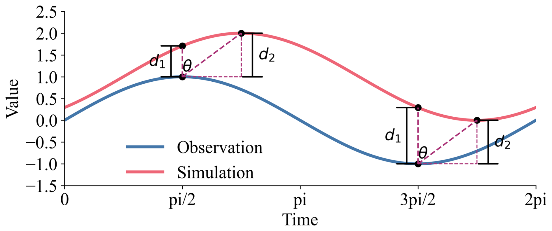
Figure 1 Geometric interpretation of the relationship between instantaneous error (d₁), phase-corrected error (d₂), and phase shift (θ). This illustrates how phase differences inflate perceived magnitude errors, thereby justifying treating phase shift as a penalty factor (PPF) applied to the accuracy component.

To quantify this scaling, we first identify the dominant phase lag (θ_lag) between the simulated and observed time series. This is achieved by applying the Fast Fourier Transform (FFT) to both series and determining the phase angle at the frequency corresponding to the maximum power in the cross-power spectrum. We define the Phase Penalty Factor (PPF) using the cosine function, which is naturally less than 1.0 (zero lag, no penalty):

$$\begin{array}{}\text{(6)}& \mathrm{PPF}=\cos \left({\displaystyle \frac{{\mathit{\theta }}_{\mathrm{lag}}}{c}}\right),\end{array}$$

where θ_lag is the dominant phase lag in radians [−π π]. The scaling parameter (c>2) is introduced to control the sensitivity of the penalty and to avoid singularity (PPF=0) if the lag approaches $\pm \mathit{\pi }/\mathrm{2}$. A smaller c imposes a heavier penalty, while a larger c reduces the impact of phase shift.

2.2.2 Capturing variability using information theory

KGE measures variability using the ratio of standard deviations ($\mathit{\alpha }={\mathit{\sigma }}_S/{\mathit{\sigma }}_O$). This ratio is susceptible to sign cancellation. For LSM data, it is highly sensitive to outliers and prone to error compensation. In other words, a model can achieve a perfect α=1 result by simultaneously overestimating and underestimating flows.

To overcome this, we utilize Shannon entropy from information theory to quantify the intrinsic uncertainty and dispersion of the data (Pechlivanidis et al., 2010). Entropy is a non-parametric measure that characterizes the shape of the probability distribution, regardless of its skewness or modality. Shannon entropy (H) is calculated from a discrete probability distribution P, obtained by binning the time series data into n_SUSE bins:

$$\begin{array}{}\text{(7)}& H\left(P\right)=-{\sum }_{k=\mathrm{1}}^{n_{\mathrm{SUSE}}}{p}_k\log \left(p_k\right)\end{array}$$

where p_k is the probability of the data falling into the kth bin. Entropy differences can be misleading if the ranges of the simulated and observed data differ significantly. Therefore, we adopt the Scaled and Unscaled Shannon Entropy differences (SUSE), which considers both the overall range and the internal shape of the distributions.

First, the scaled Shannon Entropy Difference (SED_scaled) is calculated by binning both time series using a common range from the minimum of simulations (S) and observations (O) to their maximum.

$$\begin{array}{}\text{(8)}& {\mathrm{SED}}_{\mathrm{scaled}}=|H_{S,\mathrm{scaled}}-H_{O,\mathrm{scaled}}|.\end{array}$$

Second, the unscaled Shannon Entropy Difference (SED_unscaled) is calculated by binning the time series over their respective ranges (or normalizing them first). This measures the dissimilarity of the distributions' internal shapes, independent of their absolute magnitudes.

$$\begin{array}{}\text{(9)}& {\mathrm{SED}}_{\mathrm{unscaled}}=|H_{S,\mathrm{unscaled}}-H_{O,\mathrm{unscaled}}|.\end{array}$$

The SUSE component is defined as the maximum of these two values:

$$\begin{array}{}\text{(10)}& \mathrm{SUSE}=\max ({\mathrm{SED}}_{\mathrm{scaled}},{\mathrm{SED}}_{\mathrm{unscaled}}).\end{array}$$

This ensures that the metric captures discrepancies in either the range or the shape of the variability. The number of bins (n_SUSE) serves as a sensitivity parameter, enabling comparisons across different resolutions. Setting n_SUSE=10 provides a more robust and statistically stable configuration. We recommend using the default setting (n_SUSE=10) in general evaluation and increasing n_SUSE to 100 when variability evaluation is critical.

In LSM data, moment-based statistics often suffer from excessive compression and are overly sensitive to outliers (Fig. S1). A single extreme value can cause the rejection of an otherwise good model, or conversely, a specific error pattern can make a poor model appear adequate. Information-based metrics provide a more comprehensive representation of overall distributional characteristics and are therefore less prone to such artifacts.

2.2.3 Nonparametric assessment of distribution similarity

KGE's bias term ($\mathit{\beta }={\mathit{\mu }}_S/{\mathit{\mu }}_O$) assesses the central tendency by comparing means. For non-normal streamflow data, the mean is a non-robust statistic, heavily influenced by extreme events and highly susceptible to error propagation. To provide a more comprehensive assessment of distribution similarity, we employ the Percentage of Histogram Intersection (PHI; Swain and Ballard, 1991). PHI is a nonparametric statistic that measures the overlapping area between the normalized probability distributions (histograms) of the simulated and observed data, binning the time series data into n_PHI bins:

$$\begin{array}{}\text{(11)}& \mathrm{PHI}={\sum }_{k=\mathrm{1}}^{n_{\mathrm{PHI}}}min(P_{S,k},P_{O,k}),\end{array}$$

where P_S,k and P_O,k are the probabilities of the simulated and observed data falling into the kth bin, respectively. PHI ranges from 0 (no overlap) to 1 (identical distributions). It provides a bin-by-bin assessment of the model's ability to reproduce the complete statistical signature of the observed data. It is worth noting that half of the absolute difference between probabilities is mathematically equivalent to 1−PHI. We employ the minimum in this formulation to enhance the readability of MFM framework (see Eq. 15).

2.3 MFM integration and interpretation

MFM integrates the four components (NMAEp, PPF, SUSE, PHI) into a three-dimensional Euclidean framework. To ensure commensurability, each dimension is normalized to [0, 1], where 1.0 represents the ideal value. We use the exponential transform for error and entropy components, as it provides natural and bounded normalization from [0, ∞) to (0, 1]. Additionally, the exponential transform introduces nonlinear sensitivity that prioritizes smaller errors over larger errors. This characteristic aligns with the marginal utility of model improvements (Zhou et al., 2025) while preventing extreme outliers from dominating the metric's dynamic range. The exponential transform is also a mathematical inverse of logarithmic operation in information entropy, mapping the entropy back into probability space within [0, 1].

The three dimensions of MFM are defined as:

1. Accuracy with phase penalty (ω):

   $$\begin{array}{}\text{(12)}& \mathit{\omega }=\mathrm{PPF}\times e^{-\mathrm{NMAEp}}=\cos \left({\displaystyle \frac{{\mathit{\theta }}_{\mathrm{lag}}}{c}}\right)\times e^{-\mathrm{NMAEp}}.\end{array}$$

   This component integrates magnitude error and timing accuracy. Spectral phase may be dominated by low variance background states. Evaluating phase shift in isolation overlooks timing errors in short duration extreme events, leading to overestimation, while focusing solely on extremes neglects the background state, leading to underestimation. Coupling PPF with NMAEp prevents score inflation while ensuring comprehensive timing assessment across the entire spectrum. Therefore, we integrate PPF into the accuracy dimension rather than isolating it.

2. Variability (φ):

   $$\begin{array}{}\text{(13)}& \mathit{\phi }=e^{-\mathrm{SUSE}}.\end{array}$$

   This component represents the similarity in information content and dynamic range.

3. Distribution similarity (η):

   $$\begin{array}{}\text{(14)}& \mathit{\eta }=\mathrm{PHI}.\end{array}$$

   This component represents the degree of congruence between the probability distributions.

   The final MFM score is calculated as 1.0 minus the normalized Euclidean distance from the ideal point (1, 1, 1) in this three-dimensional space:

   $$\begin{array}{}\text{(15)}& \begin{array}{rl}\mathrm{MFM}& =\mathrm{1}-{\displaystyle \frac{\sqrt{(\mathit{\omega }-\mathrm{1}{)}^{\mathrm{2}}+(\mathit{\phi }-\mathrm{1}{)}^{\mathrm{2}}+(\mathit{\eta }-\mathrm{1}{)}^{\mathrm{2}}}}{\sqrt{\mathrm{3}}}}\\ & =\mathrm{1}-{\displaystyle \frac{\mathrm{dist}\left(\right(\mathit{\omega },\mathit{\phi },\mathit{\eta }),(\mathrm{1},\mathrm{1},\mathrm{1}\left)\right)}{\sqrt{\mathrm{3}}}}.\end{array}\end{array}$$

   The distance is normalized by $\sqrt{\mathrm{3}}$ (the maximum distance from (0, 0, 0) to (1, 1, 1)) to ensure that MFM is strictly bounded within the range [0, 1]. An MFM score of 1.0 is achieved if and only if the simulation perfectly matches the observation in magnitude, timing, variability, and distribution. The decomposition into ω, φ, and η provides powerful diagnostic capabilities, allowing users to identify specific aspects of model failure.

3 Experimental design and datasets

To evaluate the robustness and diagnostic capabilities of MFM, we designed a series of experiments that compared its performance with established metrics. These experiments include targeted synthetic case studies designed to isolate known failure modes of traditional metrics, as well as an actual application using a large-sample hydrological dataset. Furthermore, we conduct a sensitivity analysis of MFM's hyperparameters.

3.1 Baseline metrics

We compare MFM against the following baseline metrics, including NSE (Eq. 2), KGE (Eq. 3), and modified KGE (mKGE, Kling et al. (2012)), which modifies the relationship between the variability and bias terms:

$$\begin{array}{}\text{(16)}& \mathrm{mKGE}=\mathrm{1}-\sqrt{(r-\mathrm{1}{)}^{\mathrm{2}}+{\left({\displaystyle \frac{\mathit{\alpha }}{\mathit{\beta }}}-\mathrm{1}\right)}^{\mathrm{2}}+(\mathit{\beta }-\mathrm{1}{)}^{\mathrm{2}}}.\end{array}$$

Additionally, we include RMSE (Eq. 1) and Normalized RMSE (NRMSE, $\mathrm{NRMSE}=\mathrm{RMSE}/{\mathit{\mu }}_O$) as direct baselines of error magnitude.

For all MFM calculations in case studies (Sect. 4.1–4.4), we use the default hyperparameters: p=1 (using NMAE for robustness), $n_{\mathrm{SUSE}}=n_{\mathrm{PHI}}=\mathrm{10}$ for both SUSE and PHI (providing a coarse-grained distribution comparison), and c=4 for the PPF (providing a moderate phase penalty).

3.2 CAMELS dataset

We apply MFM and the baseline metrics to the CAMELS dataset (Addor et al., 2017), using the Daymet forcings and corresponding streamflow observations. The CAMELS dataset is a large-sample, publicly available dataset that provides attributes and meteorological forcing for 671 catchments across the contiguous United States, specifically compiled to support the development and evaluation of hydrological and land-surface models. The Daymet dataset provides daily meteorological forcing for CAMELS. Daymet catchments have continuous runoff data spanning 34 years from 1980 to 2014, where the effects of human activity can be ignored. The model output runoff data for CAMELS were generated using a coupled model consisting of the Snow-17 and SAC-SMA models (Addor et al., 2017; Newman et al., 2015). For this study, we selected the model output files corresponding to a starting seed of 05 for consistency. We analysed daily data from 1 October 1980 to 31 December 2014. We adopted the validation criteria used by Clark et al. (2021), which states that a catchment is valid if it contains at least 10 valid years with at least 100 days of positive discharge each. We analysed the spatial distribution of the scores and examined specific catchments that highlight the diagnostic differences between the metrics.

3.3 Synthetic case studies

We designed three synthetic scenarios targeting specific metric failures.

3.3.1 Case 1: Error compensation

This case tests a metric's ability to avoid rewarding models where overestimation cancels out underestimation, a failure mode identified by Cinkus et al. (2023). We utilized a real streamflow time series (ID 01013500) from the CAMELS dataset (Addor et al., 2017) and duplicated it to create a double-length observation series (O). Two synthetic simulations are generated: (1) Bad-Good (BG) model: The first half is biased ($S_i=k_{\mathrm{1}}\times O_i$), and the second half is perfect (S_i=O_i); (2) Bad-Bad (BB) model: The first half has the same bias as BG ($S_i=k_{\mathrm{1}}\times O_i$), and the second half has a compensating bias ($S_i=k_{\mathrm{2}}\times O_i$). We first test the scenario where k₁=1.25 and k₂=0.75. Since the errors are purely proportional, the Pearson correlation (r) is 1.0 for both models, isolating the effects of the α and β components in KGE/mKGE. To test the sensitivity across different error magnitudes, we vary a scaling parameter k (from 1 to 50) and redefine the models such that the errors decrease as k increases: (1) BG model: $S_{\mathrm{first}}=\frac{k+\mathrm{1}}{k}{O}_{\mathrm{first}}$, S_second=O_second. and (2) BB model: $S_{\mathrm{first}}=\frac{k+\mathrm{1}}{k}{O}_{\mathrm{first}}$, $S_{\mathrm{second}}=\frac{k-\mathrm{1}}{k}{O}_{\mathrm{second}}$. We analysed the score difference (BG score−BB score) to determine if the metric correctly identifies BG as superior (positive difference).

3.3.2 Case 2: Stability in near-constant conditions

This case tests the stability of metrics under low-variability conditions, where normalization by small σ_O or μ_O can lead to erratic scores (Santos et al., 2018). We construct a time series of length 100 where the first 99 steps are a perfect match ($S_i=O_i=\mathrm{1}$). We then introduce a small perturbation at the final time step (i=100), with (1) Scenario A (anti-phase outlier): S₁₀₀=1.01, O₁₀₀=0.99 and (2) Scenario B (in-phase outlier): S₁₀₀=1.01, O₁₀₀=1.03. In both scenarios, the overall error magnitude (RMSE) is identical and negligible. We further test the sensitivity by iteratively increasing the magnitude of the outliers in both scenarios over 51 steps (k ranges from 0 to 50) observing the trajectory of the metrics: (1) Scenario A (anti-phase outlier): $S_{\mathrm{100}}=\mathrm{1.01}+k/\mathrm{100}$, $O_{\mathrm{100}}=\mathrm{0.99}-k/\mathrm{100}$; (2) Scenario B (in-phase outlier): $S_{\mathrm{100}}=\mathrm{1.01}+k/\mathrm{100}$, $O_{\mathrm{100}}=\mathrm{1.03}+k/\mathrm{100}$.

3.3.3 Case 3: Phase and error decoupling

This case examines how metrics balance phase errors versus magnitude errors. We design three distinct scenarios that yield the same RMSE (1.0) and NRMSE (≈1.0), but represent fundamentally different types of model failure: (1) Scenario A (extreme event): Near-constant data ($S_i=O_i=\mathrm{1.0}$ for the first 99 steps) with a single large mismatch at the end (S₁₀₀=12, O₁₀₀=2); (2) Scenario B (anti-phase): A perfectly anti-phase oscillation ($r=-\mathrm{1.0}$): $S_i=-\frac{\cos \left(i\mathit{\pi }\right)}{\mathrm{2}}+\mathrm{1}$, $O_i=\frac{\cos \left(i\mathit{\pi }\right)}{\mathrm{2}}+\mathrm{1}$; 3) Scenario C (simulation failure): Perfect phase (r=1.0) but large constant bias: $S_i=\frac{\cos \left(i\mathit{\pi }\right)}{\mathrm{100}}+\mathrm{2}$, $O_i=\frac{\cos \left(i\mathit{\pi }\right)}{\mathrm{100}}+\mathrm{1}$. We also conduct a sensitivity analysis on the reverse phase scenario (Scenario B) by varying the frequency parameter j (from 1 to 50) in the equation: $S_i=-\frac{\cos \left(i\mathit{\pi }\right)}{j}+\mathrm{1}$, $O_i=\frac{\cos \left(i\mathit{\pi }\right)}{j}+\mathrm{1}$. This gradually changes the error characteristics, allowing us to observe how metrics respond to changes in error while a constant phase error ($r=-\mathrm{1.0}$) remains.

3.4 Hyperparameter sensitivity analysis

To evaluate the robustness of the MFM with respect to its user-defined hyperparameters, a sensitivity analysis was conducted on four primary parameters: (1) Error exponent (p), varied from 1.0 (corresponding to NMAE) to 2.0 (corresponding to NRMSE) to examine the sensitivity to outliers; (2) Number of bins, varied from 5 to 100 for both SUSE (n_SUSE) and PHI (n_PHI) to assess the impact of distribution discretization resolution; (3) Phase penalty scaling factor (c), varied from 2 (indicating a heavy penalty) to 10 (indicating a light penalty) for the PPF. We perform this analysis using the CAMELS dataset results, calculating the MFM score distributions across all catchments for different parameter combinations. We analysed score variance to determine the impact of parameter choice on overall evaluation outcomes.

4 Results

4.1 Mitigate error compensation (Case 1)

The error compensation test (Case 1) reveals a failure in KGE and mKGE. In the initial scenario (k₁=1.25, k₂=0.75), both KGE and mKGE assign higher scores to the BB model than to the objectively better BG model (Fig. 2a). In contrast, MFM and NSE correctly identify the BG model as superior. The reason for this failure is evident in the KGE components (Fig. 2b). The compensating errors in the BB model (underestimation followed by overestimation) artificially pull its mean (μ_S) and standard deviation (σ_S) closer to the observed values. Consequently, the BB model achieves α and β values closer to the ideal (1.0) than the BG model. KGE and mKGE, by design, reward this statistical compensation. MFM and NSE, which incorporate direct error magnitude terms (NMAEp and RMSE², respectively), address this effect, as larger errors are always penalized more heavily, regardless of cancellation elsewhere in the time series.

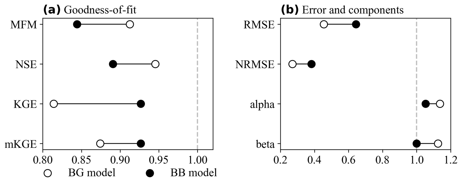
Figure 2 Error compensation results (k₁=1.25, k₂=0.75). (a) Goodness-of-fit scores. KGE and mKGE incorrectly prefer the BB model, while MFM and NSE correctly identify the BG model; (b) Error magnitudes and KGE components. The BB model's α and β are misleadingly closer to 1.0.

The sensitivity analysis across varying error magnitudes (Fig. 3) confirms the persistence of this failure. MFM and NSE consistently show a positive difference in scores, favoring the BG model. KGE remains negative, always rewarding the BB model. mKGE succeeds only at the most extreme scaling (k=1 and k=2) and fails in all other scenarios. This demonstrates that metrics relying on aggregate statistics (e.g., mean, standard deviation) for assessing bias and variability are inherently unreliable when error compensation occurs.

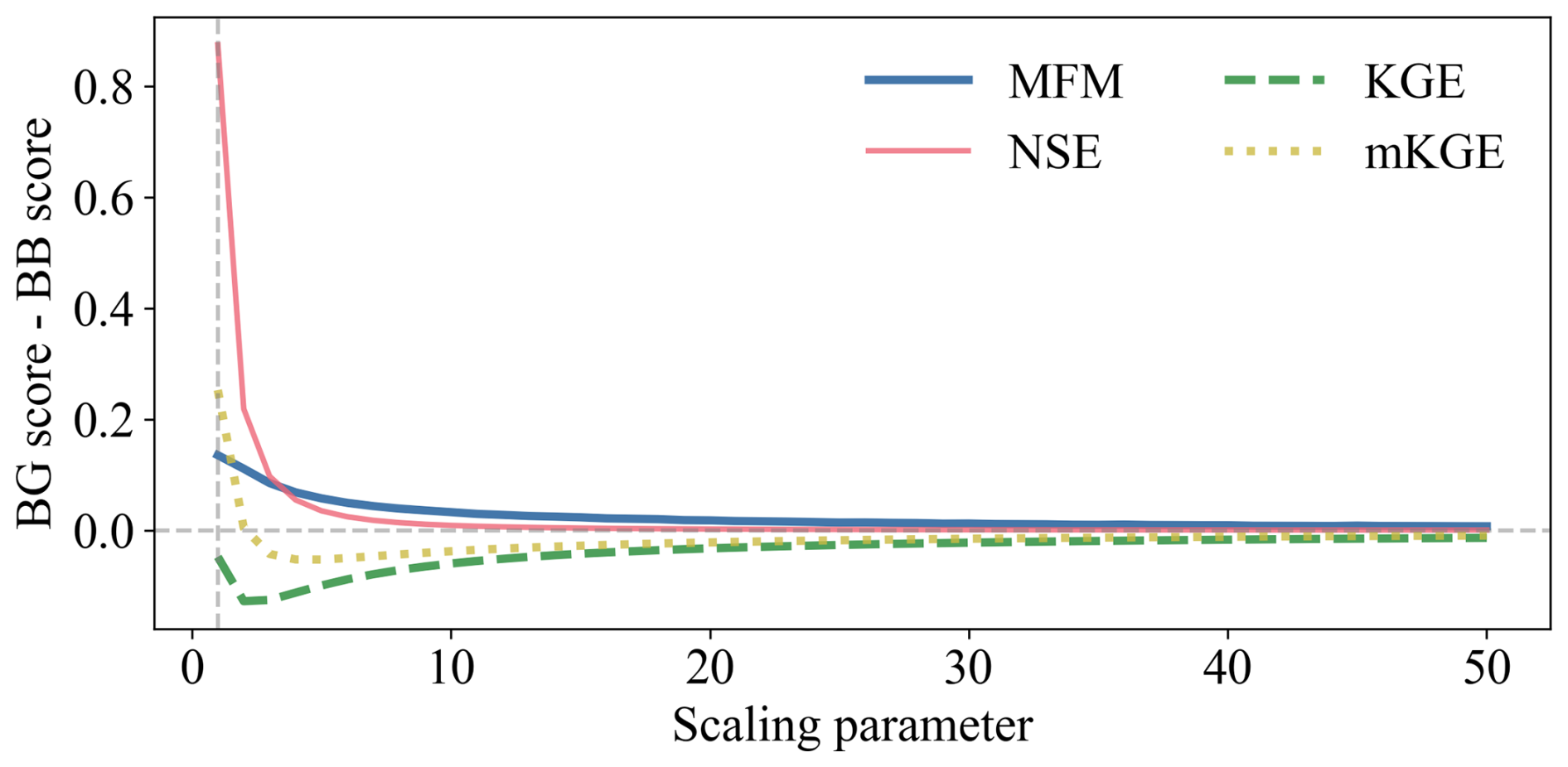
Figure 3 The difference in goodness-of-fit with different scaling parameters. The trend of metrics when the error decreases. MFM and NSE correctly distinguish BG model, while KGE fails every test. The mKGE, however, only correctly identifies the BG model when the error is large enough and fails immediately as the error shrinks.

4.2 Stability under low-variability conditions (Case 2)

The near-constant condition test (Case 2) highlights the instability of traditional metrics. In Scenario A (Fig. 4a), where a single anti-phase outlier exists, the RMSE (0.002) and NRMSE (0.002) indicate a near-perfect simulation (> 99.8 % accuracy). However, NSE (−3.04), KGE (−1.00), and mKGE (−1.00) report a failure. This instability arises because the standard deviation (σ_O) and mean (μ_O) of the observations are very small, thereby amplifying the impact of single-point errors in their normalization schemes. MFM provides a score of 0.830. This score is not near 1.0 because the PPF component successfully identified the phase reversal at i=100 and applied a penalty. If the phase penalty is disabled (PPF=1.0), the MFM score increases to 0.994, indicating an excellent magnitude match. This demonstrates MFM's stability and diagnostic capability when traditional metrics fail.

In Scenario B (Fig. 4b), where the outlier is in-phase and magnitude errors change slightly (RMSE=0.002, NRMSE=0.00199), the traditional metrics recover somewhat (NSE=0.551, KGE=0.333, mKGE=0.333), illustrating their volatility. MFM reports a near-perfect score (0.994), indicating the simulation's high fidelity.

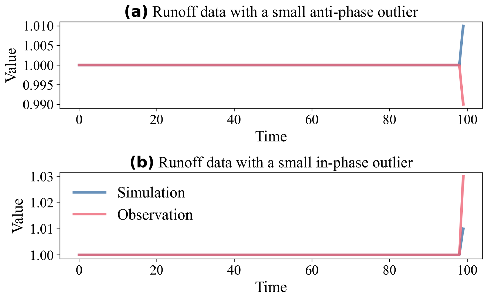
Figure 4 Stability test under near-constant conditions. (a) Scenario A: Anti-phase outlier. Traditional metrics show failure ($\mathrm{scores}\le -\mathrm{1}$) despite negligible error, while MFM provides a diagnostic score (0.830); (b) Scenario B: In-phase outlier. Traditional metrics are volatile, while MFM correctly identifies high performance (0.994).

The sensitivity analysis (Fig. 5) further emphasizes this instability. In Scenario A (Fig. 5a), as the error (RMSE) increases slightly, MFM responds with a stable, minor decrease in score (0.830 to 0.826), indicating that 99 % of the data remains perfect. NSE, KGE, and mKGE remain stuck at their initial failed values, showing no sensitivity to changes in error magnitude. In Scenario B (Fig. 5b), the RMSE remains constant. However, as the outlier magnitude increases, σ_O also increases. This change in the normalization factor causes the scores of NSE, KGE, and mKGE to rise rapidly from poor to near-perfect. Their scores reflect the changing statistical properties of the observations rather than the model performance itself. MFM remains stable and high (0.994 to 0.999), demonstrating its robustness.

Figure 5 Sensitivity analysis under near-constant conditions. (a) Scenario A: Increasing error magnitude. MFM shows a slight decrease, while baseline metrics remain insensitive at their failed values; (b) Scenario B: Constant error magnitude but increasing outlier size. Baseline metrics exhibit volatile increases attributable to changes in normalization factors, whereas MFM remains stable.

4.3 Diagnostic capability for phase errors (Case 3)

Case 3 compares three scenarios with identical RMSE (1.0) but different structural characteristics (Fig. 6). In Scenario A (extreme event, Fig. 6a), the low variability again causes the baseline metrics to fail ($\mathrm{scores}\le -\mathrm{8.0}$). MFM (0.936) is the only metric that indicates this is a generally good model, with a single significant error. In Scenario B (anti-phase, Fig. 6b), the perfect anti-correlation ($r=-\mathrm{1.0}$) leads to severe penalties by KGE (−1.00) and mKGE (−1.00). NSE (−3.0) also indicates total failure. MFM (0.572) rates the model as medium, where PPF (0.707) heavily reduces the accuracy score (ω=0.260). This medium value is caused by the variability and distribution similarity components ($\mathit{\phi }=\mathit{\eta }=\mathrm{1.0}$) recognizing the correct capture of the model. In Scenario C (simulation failure; Fig. 6c), all metrics indicate that the model is poor. However, the reasons differ significantly. NSE approaches −∞ (−9999 in the calculation) due to the combination of low variability and large error. KGE (0.00) is driven solely by the large bias ratio (β=2.0), as r=1.0 and α=1.0. MFM (0.316) provides a clear diagnosis through its components (ω=0.367, φ=1.0, and η=0.0), i.e., large magnitude error, perfect match in variability (entropy), but completely disjoint distributions.

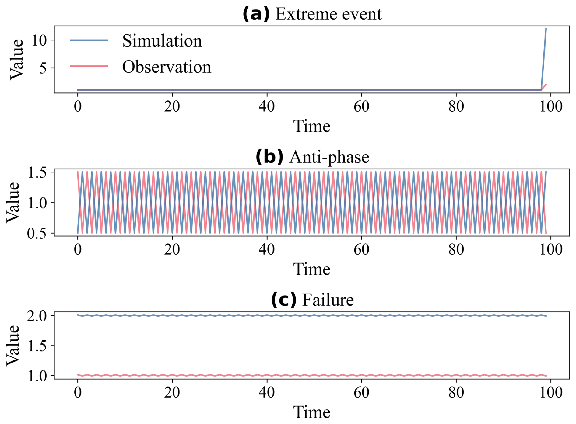
Figure 6 Phase and error decoupling test (all scenarios have RMSE=1.0). (a) Extreme event. MFM (0.936) identifies high fidelity, while baseline metrics fail ($\mathrm{NSE}=-\mathrm{100}$, $\mathrm{KGE}=-\mathrm{9.00}$, $\mathrm{mKGE}=-\mathrm{8.00}$, NRMSE=0.990); (b) Reverse phase. All metrics identify failure, driven by $r=-\mathrm{1.0}$ or PPF=0.707 (MFM=0.572, $\mathrm{NSE}=-\mathrm{3.0}$, $\mathrm{KGE}=-\mathrm{1.0}$, $\mathrm{mKGE}=-\mathrm{1.0}$, NRMSE=1.0); (c) Simulation failure, driven by large bias/error (MFM=0.316, $\mathrm{NSE}=-\mathrm{9999}$, KGE=0.0, $\mathrm{mKGE}=-\mathrm{0.118}$, NRMSE=1.0).

The sensitivity analysis of the reverse phase scenario (Fig. 7) highlights a crucial difference in the behaviour of the metric. As the oscillation characteristics change, the magnitude error (RMSE, NRMSE) decreases significantly. MFM is the only metric that responds appropriately to this improvement, with its score increasing as the error decreases. Baseline metrics remain completely insensitive, fixed at their initial low scores. This occurs because KGE and mKGE prioritize the correlation coefficient (fixed at $r=-\mathrm{1.0}$) over the actual error magnitude. MFM, by decoupling phase (via PPF) and magnitude error (via NMAEp), provides a more nuanced and reliable assessment. Given that error modes arise from multiple sources (e.g., magnitude biases, phase shifts, and temporal dynamics), a comprehensive assessment combining error metrics, correlation coefficients, and spatial error pattern maps is helpful for reliable error diagnosis.

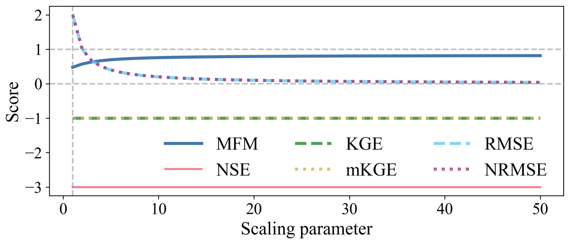
Figure 7 Sensitivity analysis of the reverse phase scenario with decreasing magnitude error. MFM correctly responds to the decreasing error, while baseline metrics remain insensitive, overly penalized by the constant anti-correlation ($r=-\mathrm{1.0}$).

4.4 Performance in real-world catchments

The application to the CAMELS dataset validates the findings from the synthetic experiments. The spatial distribution of scores (Fig. 8a–f) shows general agreement in patterns across all metrics. However, MFM exhibits a much tighter range of scores ([0.486, 0.887]) compared to NSE ([−8.43, 0.910]), KGE ([−1.47, 0.948]), and mKGE ([−1.51, 0.948]). The distribution of scores (Fig. 8g) highlights the robustness of MFM. MFM scores are centralized, whereas the distributions for baseline metrics are flatter and include extreme negative values. These extreme negative scores often reflect the undue influence of a few outliers in low-variability catchments, rather than the overall model performance, confirming the instability issues identified in Case 2 (Sect. 3.2.2). This sensitivity of baseline metrics, however, demonstrates their utility as diagnostic tools for detecting specific error modes (like reverse phase and outliers) rather than as overall performance scores.

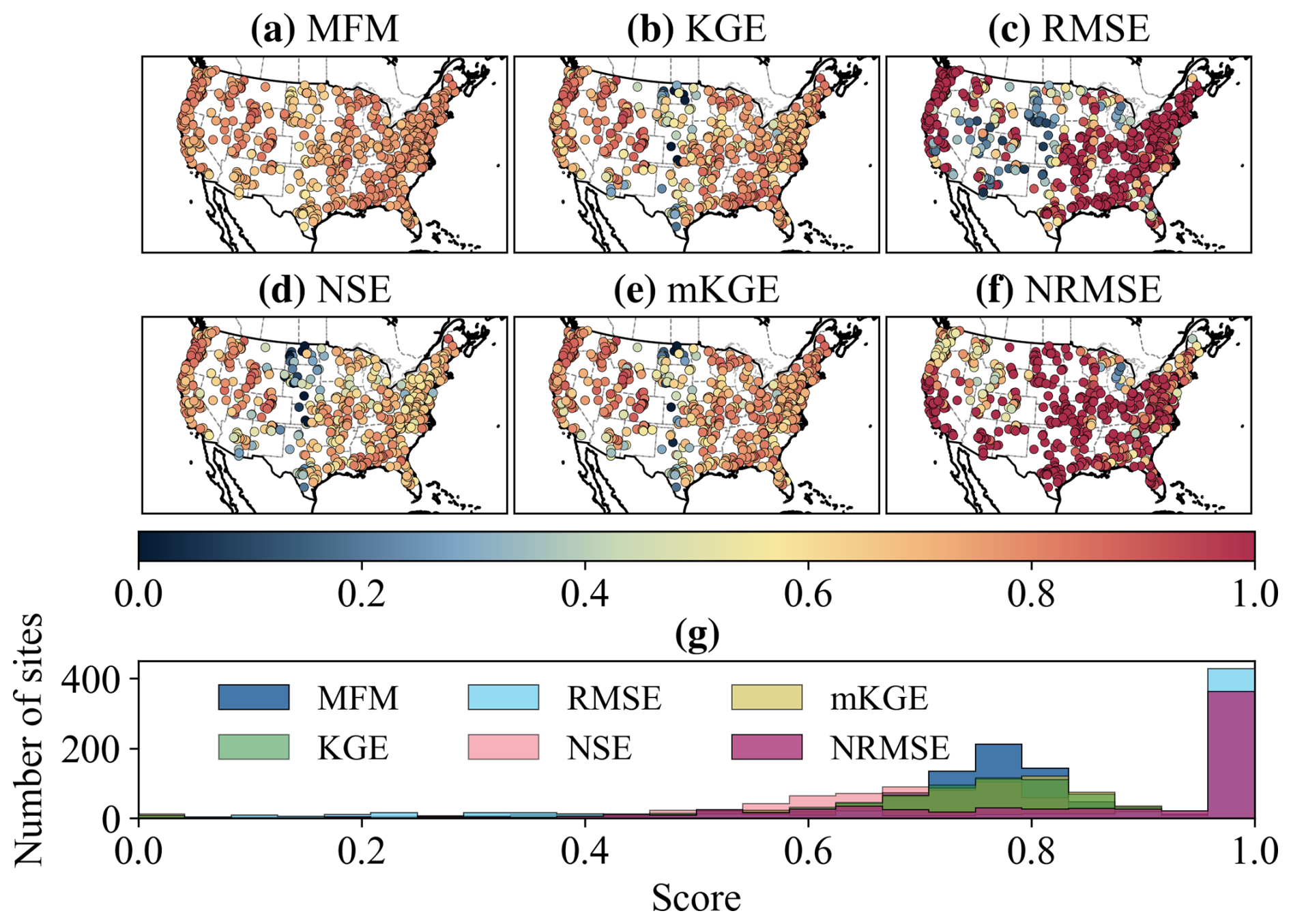
Figure 8 Spatial pattern and distribution of metrics across CAMELS dataset. (a–f) Spatial representation of MFM, KGE, RMSE, NSE, mKGE, and NRMSE; (g) Histogram of scores. MFM shows a more centralized distribution, reflecting its robustness. Baseline metrics exhibit long tails and extreme negative values.

We examine two specific catchments to illustrate MFM's diagnostic capabilities (Fig. 9). Site 05120500 (Fig. 9a) represents a low-flow, low-variability catchment (μ_O=0.0877), similar to Case 2 (Sect. 3.2.2). The simulation matches most of the observations well, but a single extreme event (April 2009) shows a large overestimation (sim=34.8 vs. obs=6.3). This single event dominates the baseline metrics, resulting in extreme negative scores ($\mathrm{NSE}=-\mathrm{8.43}$, $\mathrm{KGE}=-\mathrm{1.39}$). MFM (0.600) identifies the model as medium quality, acknowledging the large error but remaining robust. Site 06409000 (Fig. 9b) exhibits strong periodicity with a slight phase shift (FFT estimated lag≈1 d), similar to Case 3 (Sect. 3.2.3). This small lag heavily penalizes the correlation (r=0.677) due to nonlinearity, resulting in poor scores for NSE (−0.164) and KGE (0.438). MFM (0.810) identifies the model as good.

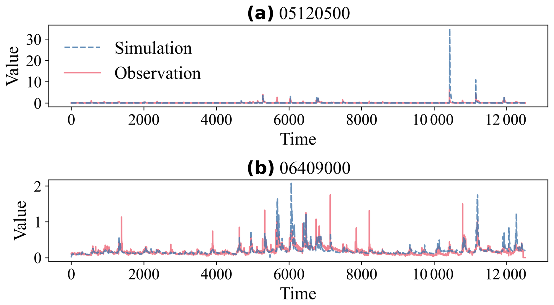
Figure 9 Time series examples from the CAMELS dataset. (a) Site 05120500. Near-constant data with an extreme event, highlighting the instability of baseline metrics; (b) Site 06409000. Data with a small phase shift but low r, highlighting MFM's ability to decouple phase and magnitude errors.

The diagnostic power of MFM is further illustrated by examining its components (Fig. 10). For site 05120500, the moderate MFM score is primarily driven by the relatively low accuracy (ω=0.319), reflecting the impact of the extreme event on the NMAEp. For site 06409000, the high accuracy (ω=0.735), the low phase lag (PPF=0.999), the high variability (φ=0.818), and distribution similarity (η=0.929) indicate that the model captures the system dynamics well, resulting in an overall good MFM score. MFM can be decomposed as shown in Fig. 10 to identify specific aspects of model failure: low ω indicates magnitude or timing errors, low φ suggests inadequate reproduction of observed variability, and low η reveals systematic distributional mismatch.

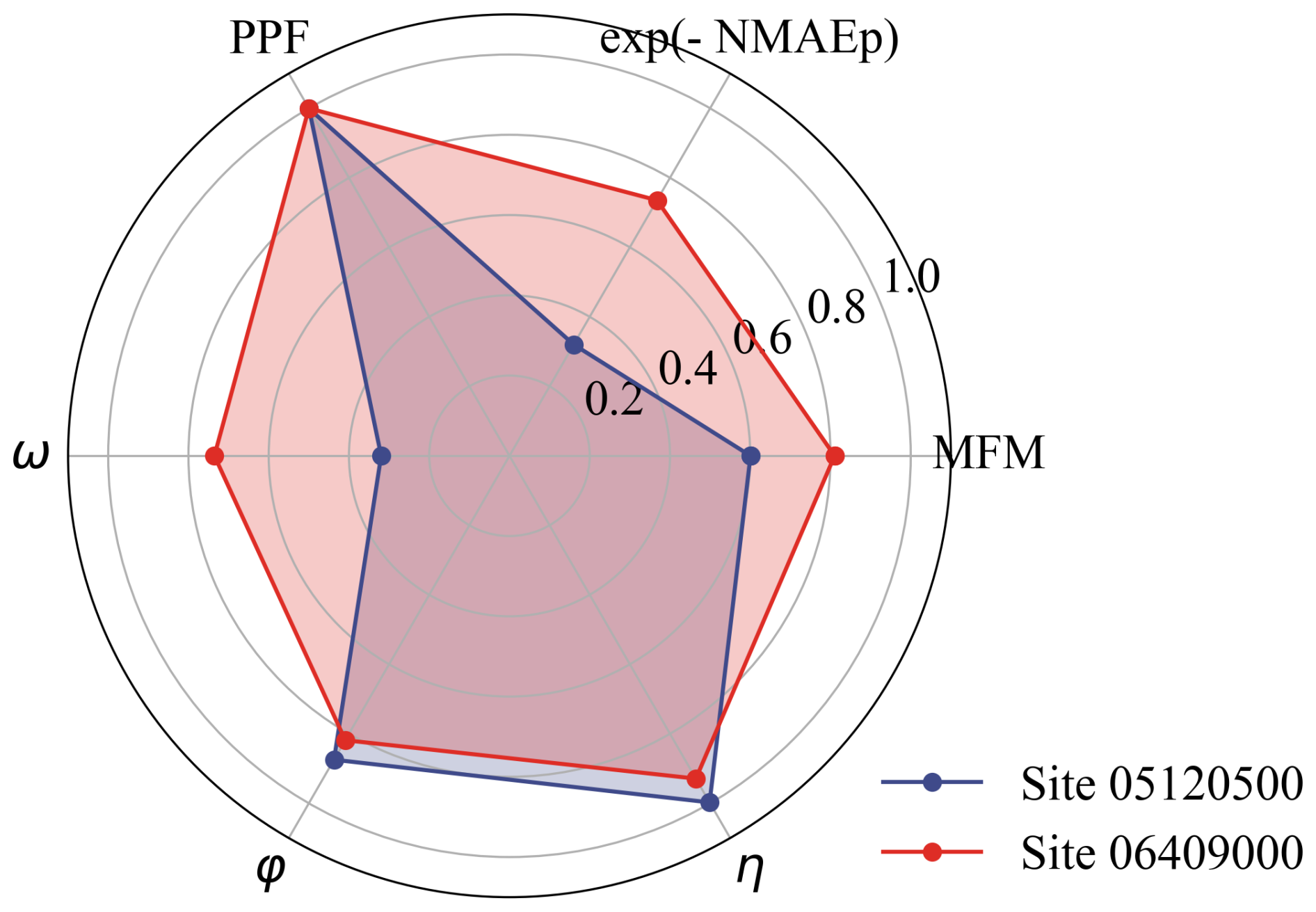
Figure 10 Radar plot illustrating the diagnostic components of MFM for the two example catchments. Site 05120500 shows relatively low accuracy (ω) due to the extreme event. Site 06409000 shows high accuracy (ω) and excellent variability (φ) and distribution similarity (η).

4.5 Sensitivity to hyperparameters

The sensitivity analysis of MFM's hyperparameters across the CAMELS dataset demonstrates its robustness to parameter choices (Fig. 11). Varying the error exponent p from 1.0 to 2.0 (Fig. 11a) results in a decrease in the MFM score, as expected, because p=2.0 (NRMSE) imposes heavier penalties on large errors compared to p=1.0 (NMAE). The overall distribution remains stable with a consistent interquartile range (IQR), indicating that the choice of p allows for transparent adjustment of sensitivity to outliers without destabilizing the metric. The number of bins for both SUSE (n_SUSE, Fig. 11b) and PHI (n_PHI, Fig. 11c) shows a high degree of robustness. Varying the bin count from 5 to 100 has a mild impact on median scores and IQR. This suggests that even a coarse discretization (e.g., the default of 10 bins) is sufficient to capture the essential characteristics of variability and distributional similarity in daily streamflow data. The phase penalty scaling factor (c, Fig. 11d) also shows a stable response. As c increases from 2 (heaviest penalty) to 10 (lightest penalty), the MFM scores slightly and smoothly increase. This indicates that, while c adjusts the severity of the phase penalty, it does not fundamentally alter the overall assessment of model fidelity.

Figure 11 Sensitivity of MFM scores across the CAMELS dataset to its four hyperparameters. (a) Sensitivity to error exponent (p). MFM scores decrease as p increases, reflecting a higher penalty for large errors; (b) Sensitivity to bins for SUSE (n_SUSE). Scores are stable; (c) Sensitivity to bins for PHI (n_PHI). Scores are stable; (d) Sensitivity to phase penalty (c). MFM slightly increases as c increases.

We recommend using p=1.0, n_SUSE=10, n_PHI=10, c=4.0 as default settings for general evaluation. When the assessment of extreme events is critical, increasing p to 2.0 imposes heavier penalties on large errors. When finer distributional resolution is needed, increasing n_SUSE and n_PHI to 100 enables percentile-level evaluation of variability and distribution similarity. Rather than introducing additional weighting parameters, adjusting these built-in hyperparameters preserves the metric's structural integrity while smoothly modulating sensitivity. Overall, the sensitivity analysis confirms that MFM is robust to its hyperparameters. The parameters provide meaningful, mathematically consistent adjustments to metric sensitivity without inducing volatility or instability observed in traditional metrics.

5 Discussion

The systematic failures of NSE, KGE, and mKGE demonstrated in our case studies (Sect. 4.1–4.3) are not isolated anomalies. They are direct consequences of relying on moment-based statistics (mean, standard deviation, and Pearson correlation coefficient) to evaluate LSM data, which are typically non-normal, skewed, and prone to outliers (Mizukami et al., 2019). The vulnerability to error compensation (Sect. 4.1) highlights the danger of inappropriately using moment-based statistics. As Cinkus et al. (2023) argued and our results confirmed, metrics that allow errors to cancel out can reward models that are “right for the wrong reasons”. MFM mitigates this effect to an acceptable extent by grounding its accuracy component (ω) in the NMAEp, which penalizes errors directly, and its distribution components (φ, η) in non-parametric methods (SUSE, PHI) that compare the entire distribution rather than summary statistics. The instability of traditional metrics under low-variability conditions (Sect. 4.2) underscores the problems inherent in their normalization schemes. When σ_O and μ_O approaches zero, these metrics become hyper-sensitive to minor fluctuations, leading to erratic and misleading scores. MFM's architecture, particularly the use of SUSE and histogram intersection (PHI), provides a stable assessment across all flow regimes, as these measures are less affected by the absolute magnitude or variance of the data. For decades, the LSM community has attempted to improve KGE by rearranging or reweighting its components (e.g., Garcia et al., 2017; Pool et al., 2018; Tang et al., 2025). While these variants can offer advantages in specific scenarios, certain inherent statistical limitations remain. MFM offers a complementary perspective, advocating the adoption of robust, information-theoretic methods appropriate to the characteristics of the data being evaluated.

This study primarily validates MFM using streamflow discharge, but its theoretical framework is designed for more LSM cases. Land surface variables, such as soil moisture, latent heat flux, and evapotranspiration, frequently exhibit periodicity, threshold behaviours, and high skewness. To address low-flow failure, traditional metrics such as NSE and KGE require a logarithmic transformation, which can introduce additional biases (Pushpalatha et al., 2012; Santos et al., 2018). In contrast, non-parametric components enable MFM to robustly quantify accuracy, variability, and pattern reproduction. This capacity makes MFM valuable for multivariate LSM evaluation.

It should be noted that, although we use the word “failure” throughout our synthetic experiments, this does not imply that baseline metrics are wrong conceptually. The unreliability we identify stems from using these metrics to quantify overall model performance in contexts where their sensitivity characteristics become liabilities rather than assets. Their high sensitivity remains advantageous for diagnosing specific error modes and assessing extreme events (e.g., Cases 2 and 3). However, when used as holistic performance scores, this same sensitivity can produce distorted results. MFM is designed to complement these metrics by providing a more stable overall score, while conventional metrics retain their role as targeted diagnostic tools.

We do not advocate for the abandonment of NSE and KGE. These legacy metrics are deeply embedded in the LSM literature and major intercomparison projects (e.g., CMIP6; Eyring et al., 2016), serving as a necessary baseline for historical comparison. However, it is crucial to distinguish between metrics used for calibration optimisation and those used for holistic model evaluation. KGE was originally designed to balance trade-offs during calibration (Gupta et al., 2009). While KGE's use as an overall evaluation metric is problematic, MFM offers a robust alternative for both purposes. MFM can serve as the objective function for calibration, or its components can be used within a multi-objective optimisation framework to achieve a balanced model performance. When comprehensive evaluation is the goal, especially under complex or extreme conditions, MFM provides a more authentic and reliable assessment.

Future LSM developments can include MFM as an overall performance score. Because it is strictly bounded within [0, 1] range and dimensionless, MFM is suitable for multi-model comparisons across different variables where variable-specific metrics fall short. MFM can also serve as an improvement constraint. To ensure that updates do not accidentally degrade overall performance, parameter calibration and coupling of new physical processes should at least maintain the MFM score. Furthermore, the evaluation of different land surface variables often demands tailored diagnostic strategies. For instance, soil moisture evaluation typically emphasizes temporal correlation and unbiased RMSE, with mean bias playing a secondary role (Entekhabi et al., 2010), whereas highly seasonal variables such as evapotranspiration and leaf area index benefit from decomposition into seasonal cycles and anomaly components for more targeted diagnosis (Mahecha et al., 2010). MFM is not intended to replace these variable-specific diagnostic approaches; rather, we recommend reporting MFM alongside fit-for-purpose metrics to provide both a reliable overall score and detailed insight into specific error modes.

While the sensitivity analysis (Sect. 4.5) demonstrated MFM's robustness to its hyperparameters (p, n_SUSE, n_PHI, c), the choice of these parameters still requires user consideration based on the specific application and data characteristics. We recommend initializing MFM with default parameters (p=1.0, n_SUSE=10, n_PHI=10, c=4.0), where NMAEp is equivalent to NMAE, coarse binning mitigates sparsity, and phase shifts incur mild penalties. For rigorous assessments of extreme events or error modes, or during multi-model comparisons where competitive models achieve close scores and are difficult to distinguish, an enhanced configuration (p=2.0, n_SUSE=100, n_PHI=100, c=2.0) is recommended. This setting equates NMAEp to NRMSE to strictly penalize large errors, employs percentile-based binning for distributional fidelity, and forces ω to 0 under anti-phase conditions via PPF.

To strengthen the interpretability of MFM and establish objective performance benchmarks (Clark et al., 2026), we conducted several calculations. We tested MFM against several naive predictive benchmarks under both default (Fig. S2) and enhanced (Fig. S3) parameter configurations. These benchmarks included the observation mean, uniformly and normally distributed random data, and percentile rankings. During these tests, the benchmark simulation sequences were sorted from smallest to largest to match the ranked observations. Additionally, we analyzed the metric's theoretical boundary conditions. If a model perfectly captures only one of the three MFM dimensions (e.g., ω=1.0, φ=0.0, η=0.0), it yields a baseline score of 0.183. If it perfectly captures two out of three dimensions (e.g., ω=0.0, φ=1.0, η=1.0), the score is 0.422. Furthermore, we derive the theoretical expectation of MFM for independent simulations (s) and observations (o) following an exponential distribution ($f\left(x\right)=\mathit{\lambda }{e}^{-\mathit{\lambda }x}$):

$$\begin{array}{}\text{(17)}& E\left[\mathrm{NMAEp}\right]={\displaystyle \frac{{\int }_{\mathrm{0}}^{\mathrm{\infty }}{\int }_{\mathrm{0}}^{\mathrm{\infty }}|s-o|{\mathit{\lambda }}^{\mathrm{2}}{e}^{-\mathit{\lambda }(s+o)}\mathrm{d}s\mathrm{d}o}{{\mathit{\mu }}_O}}={\displaystyle \frac{\frac{\mathrm{1}}{\mathit{\lambda }}}{\frac{\mathrm{1}}{\mathit{\lambda }}}}=\mathrm{1}.\end{array}$$

where E[⋅] is expectation. Under these conditions ($\mathit{\omega }=e^{-\mathrm{1}}$, $\mathit{\phi }=\mathit{\eta }=\mathrm{1.0}$) MFM = 0.635. Analogously, the enhanced MFM calculates to 0.563 ($\mathit{\omega }=e^{-\sqrt{\mathrm{2}}}$, $\mathit{\phi }=\mathit{\eta }=\mathrm{1.0}$). The exponential distribution was chosen because it is the most fundamental and easily solvable model for highly skewed LSM variables. Consequently, surpassing this threshold indicates that the model outperforms purely stochastic systems which share the exact same statistical distribution. The superior threshold 0.8 was defined to filter out nearly all simple benchmarks, including mean, randomly distributed, and 10-bin benchmarks. As shown in Figs. S2 and S3, while 47 % of the 100-bin benchmark crossed the 0.8 line, only 2 % of the enhanced setting reached this level.

To simplify usage, the benchmark thresholds are defined as 0.2, 0.4, 0.6, and 0.8. Scores within [0.0,0.2] are deemed unacceptable, indicating outliers. Range (0.2,0.4] is classified as poor, where the model equivalently captures at most one dimension correctly. Medium range is defined as (0.4,0.6], indicating the model equivalently captures at least two dimensions. Scores in (0.6,0.8] are considered as good, reflecting strong overall performance across accuracy, variability, and distribution. Finally, the (0.8,1.0] range represents superior performance, characterized by near perfect fidelity.

The calculation of MFM (involving FFT, entropy estimation, and histogram) is computationally more intensive than KGE or NSE. This may pose a challenge for applications that require millions of model evaluations, such as intensive Monte Carlo simulations or complex optimisation routines. A critical direction for future work is the integration of uncertainty estimation. A metric score is only meaningful if its statistical reliability is understood (Schaefli and Gupta, 2007). The reliance on observational data, which often contains significant uncertainty, further complicates model evaluation (Moriasi et al., 2007; Refsgaard et al., 2007). We have integrated MFM within uncertainty estimation frameworks, such as the gumboot package (Clark et al., 2021) and the Open Source Land Surface Model Benchmarking System (OpenBench, Wei et al., 2025), to provide confidence intervals for MFM scores. This will enable a more rigorous assessment of model performance, moving beyond deterministic scoring towards a probabilistic evaluation (Vrugt et al., 2022).

6 Conclusion

Evaluating LSMs requires metrics that are robust, diagnostic, and reliable across diverse conditions. Traditional metrics like NSE and KGE are appropriate for identifying specific problems in LSMs. However, when used as overall scores in performance evaluation, they have fundamental limitations stemming from their reliance on moment-based statistics that are ill-suited to the non-normal, skewed nature of LSM data. These flaws can lead to error compensation, instability in low-variability conditions, and inadequate treatment of phase errors, resulting in misleading model evaluations. To address these fundamental limitations, we introduced the MFM, a comprehensive performance criterion derived from first principles, employing robust statistics and information theory. MFM fundamentally reconstructs the evaluation framework, replacing KGE's components with three orthogonal dimensions of model fidelity. It integrates a robust measure of accuracy (NMAEp) penalized by timing errors (PPF), captures variability using information entropy (SUSE), and assesses distribution similarity nonparametrically (PHI). Through targeted synthetic experiments and application to the CAMELS dataset, we demonstrated that MFM provides a more authentic and reliable assessment of model performance than traditional metrics. MFM mitigates error compensation, remains stable under low-variability conditions in which NSE and KGE fail, and provides powerful diagnostic insights by decomposing performance into its core components. MFM represents a significant advancement in LSM evaluation. We advocate a transition from the community's reliance on traditional metrics toward more robust, diagnostic frameworks, for which MFM serves as a powerful, reliable alternative, supporting the development of more trustworthy LSMs.