Leveraging 20 years of remote sensing to characterize surface phytoplankton seasonality and long-term trends in lake Tanganyika

Lake Tanganyika, the world's second-largest freshwater lake by volume, is a vital resource for millions in East Africa, providing water, food, and economic opportunities while supporting exceptional biodiversity.

Chlorophyll a concentration (Chl a) is a key indicator of phytoplankton biomass. In Lake Tanganyika, Chl a is known to display strong spatiotemporal horizontal variability with an exceptionally low annual mean and wide ranges of concentrations compared to other tropical or temperate great lakes. This variability is influenced by the lake's hydrodynamic cycle driven by air temperature and wind seasonality. Phytoplankton biomass is suspected to be decreasing due to a strengthening of water column stratification induced by climate change. However, the particular spatiotemporal variability and trends in phytoplankton biomass have never been examined using a lake-wide, temporally continuous long-term record. This study bridges this gap by analyzing satellite remote sensing-derived Chl a data from the ESA Climate Change Initiative Lakes dataset across the entire surface of Lake Tanganyika over a 20-year period. It offers insight into the Chl a dynamics with an unprecedented timespan and spatial coverage.

The analysis reveals distinct seasonal patterns in Chl a concentrations, with shallow regions (depth < 170 m) maintaining higher levels year-round, while deeper areas exhibit pronounced seasonality tightly linked to known wind patterns. To further explore these spatial differences in seasonal dynamics, the study identifies seven clusters of co-varying Chl a concentrations, each displaying distinct seasonal behaviours that reflect the lake's hydrodynamic cycle. Long-term trends indicate a decline in Chl a concentrations of −9 % per decade in deep regions, suggesting decreasing phytoplankton biomass. However, this overall decline is nuanced by monthly patterns. In deep regions, the low Chl a concentrations, mainly observed between November and April, tend to decrease over time at rates between -5 to −15 % per decade when averaged over entire clusters. In contrast, highest Chl a values recorded during the most productive months, from August to October, show increasing trends up to 25 %. Nearly all shallow areas, meanwhile, display year-round increases up to 35 % across the Chl a distribution, with particularly sharp rises in extreme values.

The findings underscore the complexity of Lake Tanganyika's Chl a dynamics. The observed trends may have significant consequences for the lake's trophic structure and the communities dependent on its resources. Further research is needed to elucidate the underlying drivers of these changes and to assess their broader ecological and socio-economic impacts.

1 Introduction

Lakes play a fundamental role in global biogeochemical cycles and provide essential ecosystem services, serving as crucial water resources for millions of people (Wetzel, 2001). However, these fragile ecosystems face increasing pressure from climate change, pollution and other stressors, which drive profound changes in their physical, chemical, and biological properties (Brönmark and Hansson, 2002). Given their sensitivity to environmental shifts, lakes are often considered sentinels of change, rapidly responding to alterations in temperature, precipitation, and human-induced disturbances (Adrian et al., 2009; Williamson et al., 2009). Continuous monitoring of water quality is essential to better understand these ecosystems, for assessing the transformations they are undergoing and guiding adaptive management efforts.

One important indicator of lake ecosystem dynamics is phytoplankton biomass (Xu et al., 2001). Variations in phytoplankton biomass can signal shifts in trophic state, alterations of ecosystem dynamics, or direct anthropogenic pressures such as water pollution. Since phytoplankton form the base of the aquatic food web, fluctuations in their abundance directly influence higher trophic levels and therefore the whole ecosystem (Wetzel, 2001). Measurements of phytoplankton concentration are typically made at discrete locations, either via boat campaigns or from easily accessible buoys (Kutser, 2009; Lombard et al., 2019). However, in large bodies of water, such methods may not adequately represent the overall water quality across the entire surface. Additionally, temporal availability can present challenges, as these methods are often limited in sampling frequency. In recent decades, the use of optical satellite remote sensing to estimate phytoplankton biomass has emerged as a powerful tool, providing broad spatial coverage and continuous temporal monitoring across large water bodies (Gordon and Wang, 1994; Hu and Campbell, 2014; Martin, 2014; McClain et al., 2006; Moore et al., 2014; Moses et al., 2009; Neil et al., 2019). It involves estimating chlorophyll a (Chl a) concentration by utilizing its distinctive absorption peaks in the blue and red bands (Martin, 2014).

Lake Tanganyika, located in East Africa, is the second most voluminous freshwater lake in the world. It spans four countries, Tanzania, the Democratic Republic of the Congo, Burundi, and Rwanda. It is an essential resource for millions of people living along its shores, who rely on the lake's fish as their primary source of animal protein but also for water and economic opportunities (Bulengela, 2024; Mölsä et al., 2002; Niyongabo et al., 2024; Paffen et al., 1997). The lake is characterized by its unique ecosystem, which supports a wide range of endemic species, particularly in its fish communities (Coulter, 1991). This ecosystem is increasingly exposed to a multitude of threats as climate change poses significant challenges, exacerbated by human activities (Plisnier et al., 2018). Extreme high water levels in recent years have had severe consequences, causing floods and population displacements (Gbetkom et al., 2024; Papa et al., 2023). Physical parameters of the lake are changing such as water temperature that increases along with air temperature, causing a strengthening of vertical stratification (O'Reilly et al., 2003; Verburg et al., 2003). This increased stratification is expected to reduce nutrient upwelling, thereby limiting phytoplankton growth, the key driver of the lake's food web and fisheries. Reduction in vertical mixing has caused the oxycline to rises, restricting habitats to shallower areas (Cohen et al., 2016; Van Bocxlaer et al., 2012).

Lake Tanganyika's water quality and ecosystem dynamics have been the focus of numerous studies, many of them focusing on primary production and phytoplankton concentrations (Bergamino et al., 2007, 2010; Corman et al., 2010; Descy et al., 2005; Hecky and Fee, 1981; Hecky and Kling, 1981; Langenberg et al., 2002; Stenuite et al., 2007). Field campaigns have usually focused on specific regions of the lake, often nearshore and during limited time periods (Plisnier, et al., 2023). Phytoplankton concentrations in the lake are generally low but they exhibit high spatial and temporal variability, making it challenging to characterize their lake-wide dynamics with sparse in situ measurements. Satellite remote sensing provides a complementary approach. Horion et al. (2010) validated a MODIS-based algorithm for estimating Chl a concentrations in Lake Tanganyika using in-situ measurements collected between 2002 and 2006. The algorithm applied in their study is similar to the one used in the lakes_CCI processing chain, which ensures consistency with that validated approach in the context of our study. Bergamino et al. (2010) then used MODIS remote sensing data based on Horion's algorithm to estimate annual primary production over the entire lake surface based on three years of observations. Their study was limited to a short time series and did not characterize seasonal variability or assess long-term trends in phytoplankton dynamics. No study to date has provided a comprehensive, long-term assessment of phytoplankton dynamics across the entire lake surface, preventing a full understanding of spatial patterns, seasonal cycles, and long-term trends.

This study aims to analyse the spatiotemporal variability of surface Chl a concentrations across the entire surface of Lake Tanganyika, with particular attention to regional differences in seasonal dynamics. We also seek to assess long-term trends over the past two decades and examine changes in the statistical distribution of Chl a, with an emphasis on extreme values. Finally, we aim to compare Chl a trends between deep and shallower zones of the lake to identify potential differences in their responses to environmental and climatic drivers.

2 Material and Methods

2.1 Study Site

Lake Tanganyika is the largest African Great Lake, located between −3.6 and −8.8° N and 29.2 and 31.2° E (Fig. 1). It is 650 km long, averaging 50 km of width along a North-West to South-East axis and has an area of more than 32 600 km². It comprises three main basins, with the deepest point reaching 1400 m located in the central basin.

The region's climate is characterized by a pronounced wet season from September to April, with average annual precipitations of approximately 1000 mm. Air temperatures are relatively stable, typically ranging between 25 and 29 °C. Strong southeast winds peak in July–August before weakening in September as the Intertropical Convergence Zone shifts (Nicholson, 2000), while lighter northerly winds dominate the rest of the year (Coulter, 1991).

Surface water temperatures vary seasonally between 24 to 28 °C while deep-water temperatures remain stable at 23.45 °C. Lake Tanganyika is highly stratified and meromictic, meaning its water column never fully mixes (Coulter, 1991). Seasonal monsoon winds dominate the mixing processes. During the dry season (May–August), strong southeast winds tilt the thermocline, causing it to rise closer to the surface in the south. This disruption of stratification in the south favors upwellings, which enhance nutrient cycling and promote phytoplankton growth. Simultaneously, surface waters are pushed northward, causing downwelling in the northern basin. As winds relax during the wet season transition (September–October), stratification returns in the south while secondary upwellings occur in the north. Internal seiching, a lake-wide oscillation of the thermocline, becomes prominent, driving mixing and primary production especially when its amplitude reaches surface waters (Corman et al., 2010; Coulter, 1991; Langenberg et al., 2002, 2003; Naithani et al., 2002; Plisnier et al., 2023b, 1999; Plisnier and Coenen, 2001).

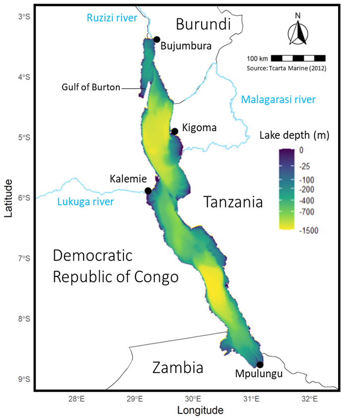
Figure 1 Map of Lake Tanganyika bathymetry, surrounding countries, major towns, and key rivers (Inflow: Ruzizi, Malagarasi; Outflow: Lukuga).

Lake Tanganyika's water is remarkably clear, ithan average Secchi disk depth transparency of around 12 m (Plisnier et al., 2015). Nutrient levels at the surface are generally low. Phytoplankton concentration show great spatiotemporal variability depending on the nutrient availability in the euphotic zone. The seasonality of phytoplankton concentration, often measured in terms of Chl a levels or estimates of primary production, depends on the hydrodynamic cycle and winds seasonality. Phytoplankton biomass is located between depths from 0 to 40 m with maxima commonly found between 0–20 m (Descy et al., 2010; Salonen et al., 1999; Vuorio et al., 2003). Bergamino et al. (2010) used remote sensing data from 2002 to 2005 to estimate primary productivity over the whole lake's surface based on MODIS data. They computed an average of 646 ± 142 mg C m⁻² per day. They also showed the remarkable differences between some coastal zones around the lake in shallower areas showing values above 800 mg C m⁻² per day and the rest of the lake where primary production was lower. The lake's stratification regime has indeed confined the distribution of benthic organisms to a narrow band of biodiversity around the lake within the upper, oxygen-rich water layer (Van Bocxlaer et al., 2012).

Lake Tanganyika has experienced significant warming, with recent temperature increases unprecedented in the past 1500 years (Tierney et al., 2010). Since 1913, the upper water column has warmed at approximately 0.1 °C per decade (Kraemer et al., 2015; O'Reilly et al., 2003), with higher rates in the north due to weaker vertical mixing. Seasonal variations exist, with slower warming during the dry season (0.08 °C per decade) and faster warming near the shore (Verburg and Hecky, 2009). This warming trend is expected to increase the stability of the water column and reduce vertical mixing (O'Reilly et al., 2003; Tierney et al., 2010; Verburg et al., 2003; Verburg and Hecky, 2009).

Direct measurements of primary production have been too intermittent to determine whether the changes in the lake have caused a decrease in productivity (Macintyre, 2012). O'Reilly et al. (2003) suggested a 20 % decline in primary productivity and a 30 % reduction in fish yields based on carbon isotope records from sediment cores. Reduced silica demand by diatoms further indicates a shift toward a more oligotrophic system (Verburg et al., 2003; Verburg and Hecky, 2009). Stenuite et al. (2007) reported daily mean and daily minimum primary production below previous estimates while Bergamino et al. (2010) estimated primary productivity in 2003 using remote sensing data and found a 15 % decrease compared to the estimate by Hecky and Fee (1981), though the studies used different methodologies.

An increase in water temperature is also expected to reduce the mixing and oxycline depths, reducing ecosystem habitats (Cohen et al., 2016; O'Reilly et al., 2003; Verburg et al., 2003). Indeed, if vertical mixing is reduced, the oxygen consumed by metabolic respiration cannot be replenished through mixing, leading to its depletion. This should cause a narrowing of the ring of benthic biodiversity in the lake. Concurrently, water clarity has improved as phytoplankton levels have declined. This could enhance benthic primary production relative to that of pelagic phytoplankton (Van Bocxlaer et al., 2012). All these environmental changes are coupled with observations of declining fish populations even before the era of commercial fishing (Cohen et al., 2016).

2.2 Dataset

We used the ESA Climate Change Initiative Lakes dataset (Lakes_cci Version 2.1) (Carrea et al., 2024).This dataset contains Essential Climate Variables (ECV) such as lake water level and extent, lake surface water temperature (LSWT), Chl a and water turbidity for over 2000 lakes worldwide. The Chl a coverage spanned from 2002 to 2022, with a theoretical daily temporal resolution, that may vary due to cloud cover, and a spatial resolution of 1/120th of a degree of latitude. This roughly corresponds to a spatial resolution of 1 km near the equator. Data from different satellite products (MERIS on Envisat, MODIS on Terra and Aqua, and OLCI on Sentinel-3) were harmonized to produce a temporally consistent Chl a dataset. The Lakes_cci dataset also provides uncertainties layers associated with each ECV. For Chl a, 90 % of the dataset had an associated fractional uncertainty between 39 and 60 %. MODIS data was not released for most lakes in the dataset including Lake Tanganyika. The dataset therefore shows a data gap during the 2012 to 2016 period.

2.3 Data Interpolation Method

Due to cloud cover and satellite revisit times, the dataset contains gaps, with some days missing data entirely or having incomplete coverage of the lake. To address this, we applied an interpolation method to fill in missing data and ensure continuity in the analysis. The Data Interpolating Empirical Orthogonal Functions (DINEOF) technique was used for spatio-temporal interpolation of Chl a and LSWT data (Alvera-Azcárate et al., 2005; Beckers and Rixen, 2003). The method consists in iteratively decomposing and reconstructing the dataset in a set of empirical orthogonal functions (EOF), expressed as spatial and temporal modes. This process is repeated until the root mean square error, computed on a spatially coherent set of validation pixels, converges to a stable value. These validation pixels were selected as contiguous areas of 10 000 pixels from the 15 images with the least cloud coverage in the dataset. We found 7 to be the optimal number of EOF modes that minimizes the error function. We applied this interpolation procedure solely to images containing less than 95 % missing values, as recommended by the method. Other images were not altered and remained in the dataset in their original state.

2.4 Analysis methods for Seasonal and Interannual Variations of Chlorophyll a

To capture the seasonal dynamics of surface Chl a concentrations, we first generated monthly median maps of Chl a by computing the median of all values observed during each month at each location. These maps illustrate the general spatial patterns of Chl a across the lake. However, they cannot be used to display the short-term and interannual variability in Chl a.

To address this limitation and provide a more detailed characterization of the temporal variability of Chl a in Lake Tanganyika, we partitioned the lake into regions with co-varying Chl a concentrations rather than analysing the lake as a whole. To do the partitioning, we used k-means clustering (MacQueen, 1967) with the seven spatial empirical orthogonal function modes previously computed using the DINEOF method as input. The optimal number of spatial clusters, determined using the silhouette value (Rousseeuw, 1987), was found to be 7. To characterize the temporal variability of Chl a, we computed two complementary time series for each cluster. The first captures the interannual variability of Chl a, calculated as the 10th, 25th, 50th, 75th, and 90th quantiles of all observations for each month between January 2002 and December 2022. The second time series represents the seasonal cycle of Chl a and is calculated as the 10th, 25th, 50th, 75th, and 90th quantiles of all Chl a estimates within each cluster for each day of the year, pooling data across all years in the time series. This means that each day's statistics represent interannual daily percentiles, derived from the corresponding day across all years in the dataset. We had first applied a five-day rolling mean to the time series of each pixel over the entire period from 2002 to 2022. This smoothing method was selected to reduce the impact of outliers, minimize the influence of missing data while preserving short-term variability, following the approach of Laliberté and Larouche (2023).

Chl a trends were independently calculated for each pixel across Lake Tanganyika using daily time-step data from the lakes_cci dataset for the period 2002 to 2022. Before conducting the trend analysis, we first removed the seasonal cycle. To do this, we determined the interannual median Chl a value for each pixel i on each day of the year (DOY), averaging across all years in the time series. These seasonal cycles were then smoothed using a 5 d rolling mean. Finally, Chl a anomalies were calculated by subtracting the smoothed seasonal values from the observed Chl a concentrations following Eq. (1), ensuring that the trend analysis focused on long-term changes rather than recurring seasonal fluctuations.

$$\begin{array}{}\text{(1)}& \mathrm{Chl}a{A}_{i,t}=\mathrm{Chl}{a}_{i,t}-{\stackrel{\mathrm{̃}}{\mathrm{Chl}a}}_{i,\mathrm{DOY}},\end{array}$$

where Chl a_i,t is the observed Chl a concentration for pixel i on day t, with i=1, …, N (the total number of pixels covering the lake) and t representing the day number within the period from January 1, 2002, to December 31, 2022. ${\stackrel{\mathrm{̃}}{\mathrm{Chl}a}}_{i,\mathrm{DOY}}$ is the interannual median Chl a concentration for pixel i on the corresponding DOY, averaged across all years, and smoothed using a 5 d rolling mean. Chl a A_i,t represents the deviation of the observed Chl a from the expected seasonal median value.

Overall Trends in Chl a were calculated using the Sen's slope estimator $\stackrel{\mathrm{̃}}{\mathit{\beta }}$ following Eq. (2), expressed in mg m⁻³ per decade, alongside a Mann-Kendall test for significance. The Sen's slope, defined as the median of all pairwise slopes in the time series (Sen, 1968), provides a robust estimate of trend magnitude.

$$\begin{array}{}\text{(2)}& {\stackrel{\mathrm{̃}}{\mathit{\beta }}}_i=\mathrm{median}\left({\displaystyle \frac{\mathrm{Chl}a{A}_{i,t_j}-\mathrm{Chl}a{A}_{i,t_k}}{t_j-t_k}}\right)\text{for all}{t}_j>t_k,\end{array}$$

where Chl $a{A}_{i,t_j}$ and $\mathrm{Chl}a{A}_{i,t_k}$ are the Chl a anomalies for pixel i at times t_j and t_k, respectively.

Firstly, overall absolute trends were computed for each pixel using all available observations and are expressed as changes in surface Chl a concentration per decade. Overall relative trends were then computed by dividing the overall absolute trends by the median Chl a concentration at each pixel following Eq. (3), providing a relative measure of change, expressed in percentage by decade.

$$\begin{array}{}\text{(3)}& \mathrm{relative}{\stackrel{\mathrm{̃}}{\mathit{\beta }}}_i={\displaystyle \frac{{\stackrel{\mathrm{̃}}{\mathit{\beta }}}_i}{\stackrel{\mathrm{̃}}{\mathrm{Chl}a{A}_i}}},\end{array}$$

where $\stackrel{\mathrm{̃}}{\mathrm{Chl}a{A}_i}$ is the median Chl a concentration anomaly at pixel i over the study period.

To capture intra-annual variations of these trends, monthly relative trends were also estimated using only the observations for each specific month of the year.

2.5 Partition and Shifts in Chlorophyll a Distribution

In addition to analysing overall and monthly trends per pixel, we assessed if there was any shift in yearly statistical distribution of Chl a over time. To achieve this, we computed trends for a set of yearly quantile values, consisting of those at 2.5 % intervals along with the uppermost quantiles at 98 %, 98.5 %, 99 %, 99.5 %, and 99.9 %. Recognizing that lake-wide trends might obscure local variability, we conducted this analysis within the seven previously defined clusters of similar temporal Chl a variability. For each pixel, we calculated all yearly quantile values and determined trends from 2002 to 2022 using the Sen's slope estimator following Eq. (4). Relative trends were then calculated by dividing each yearly quantile trend by its interannual mean, yielding rates of change. Finally, we spatially aggregated the results by calculating the median rate of change for each quantile within each cluster following Eq. (5).

$$\begin{array}{}\text{(4)}& {\displaystyle }{\stackrel{\mathrm{̃}}{\mathit{\beta }}}_{q,i}=\mathrm{median}\left({\displaystyle \frac{q_{i,y_j}-q_{i,y_k}}{y_j-y_k}}\right),\text{(5)}& {\displaystyle }\mathrm{relative}{\stackrel{\mathrm{̃}}{\mathit{\beta }}}_{q,C}=\mathrm{median}\left({\displaystyle \frac{{\stackrel{\mathrm{̃}}{\mathit{\beta }}}_{q,i}}{{\stackrel{\mathrm{‾}}{q}}_i}}\right)\forall i\in C,\end{array}$$

where ${\widehat{\mathit{\beta }}}_{q,i}$ is the Sen's slope estimator for the qth quantile, calculated as the median of pairwise slopes between yearly quantile values $q_{i,y_j}$ and $q_{i,y_k}$ for pixel i over years y_j and y_k between 2002 and 2022. $\mathrm{relative}{\stackrel{\mathrm{̃}}{\mathit{\beta }}}_{q,C}$ is the median rate of change for the q^th quantile within a specific cluster C , calculated based on all pixels i within this cluster. ${\stackrel{\mathrm{‾}}{q}}_i$ is the interannual mean of qth quantile at pixel i across all years. This analysis was conducted separately for pixels in deep and shallower zones, as these two areas are influenced by distinct processes influencing Chl a concentrations.

3 Results

3.1 Seasonality of Chl a Concentrations

The maps of interannual monthly median surface Chl a shown in Fig. 2 highlight strong differences between some coastal zones and the rest of the lake. These coastal zones usually extend a few kilometres offshore and are relatively shallow, with depths generally not exceeding 250 m (Fig. 1). They exhibit consistently higher median concentrations throughout the year, above 3 mg m⁻³ in some areas. In contrast, open waters with greater depths and deep nearshore zones exhibit a more pronounced Chl a seasonality, displaying low median levels outside the productive season between January and April, below 0.3 mg m⁻³.

Shallow zones with year-round higher Chl a levels are scattered around the lake. The northern zone, off the coast of Bujumbura and the Bujumbura Rural Province, feature an extensive shallow area where depths of less than 100 meters stretch up to 6 kilometres offshore. It is characterized by consistently elevated Chl a concentrations, which also extend further south along the gently sloped shores of Burundi. The Gulf of Burton, located south of Baraka on the north-western coast, shares similarities with the waters off Bujumbura, featuring a large shallow zone with sustained higher Chl a levels compared to deeper areas.

The coastal area south of Kigoma spans 700 km² at depths of less than 200 m, including 400 km² shallower than 100 m. It remains highly productive throughout the year. Some of the highest Chl a concentrations in Lake Tanganyika are observed at the Malagarasi river's estuary where a 40 km² area near the river mouth exhibits mean Chl a levels exceeding 3 mg m⁻³. Other remarkably productive regions include the shallow zones near Kalemie and the southeastern Gulf in the DRC as well as areas near Mpulungu in Zambia.

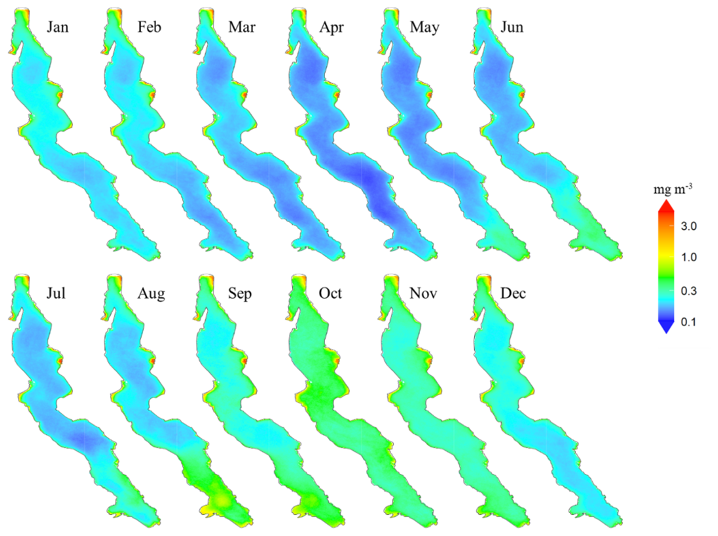
Figure 2 Maps of interannual monthly median surface chlorophyll a concentrations in Lake Tanganyika (2002–2022).

By contrast, the Tanzanian coast north of Kigoma, where depth sharply increases offshore, shows Chl a levels and seasonality comparable to that of the pelagic waters at this latitude. Similar patterns are observed along the DRC coast, both north of Kabimba and north of the border with Zambia, for example. Pelagic areas and deeper nearshore zones of the lake display monthly median surface concentrations below 1 mg m⁻³ with the lowest median levels between 0.1 and 0.3 mg m⁻³ observed in April. Chl a levels start rising in the southern regions of the lake in April and this increase gradually progresses northward in the following months, reaching the northern areas only by September. Peak concentrations are typically observed between August and November in the south and between October and November in the north. From December to April, Chl a concentrations progressively decrease across the entire lake, starting from the south.

3.2 Spatial Clustering for Improved Characterization of Chl a variability

Figure 3 illustrates the spatial aggregations into clusters of co-varying Chl a concentrations that divide Lake Tanganyika from north to south into six relatively spatially coherent regions. Cluster 7 stands out as it groups pixels from shallow coastal regions across the lake, all characterized by consistently higher Chl a levels throughout the year.

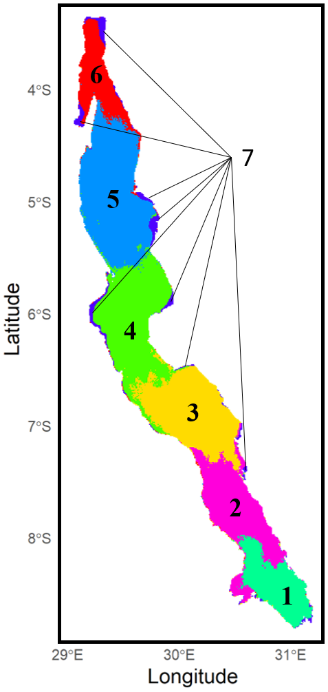
Figure 3 Clustering of Lake Tanganyika into regions of co-varying chlorophyll a concentrations with k-means clustering method.

Chl a observations within each cluster were aggregated to visualize both interannual variability and seasonal patterns. The left panel in Fig. 4 highlights substantial interannual variability across all clusters. Clear seasonal patterns emerge in clusters 1 to 6, characterized by alternating periods of lower and higher phytoplankton biomass. However, the timing of peak Chl a concentrations within the productive season varies from year to year, and multiple peaks may occur within a single year. The magnitude of these peaks also fluctuates greatly between years. In contrast, cluster 7, which represents the shallow coastal zones surrounding the lake, is characterized by persistently higher Chl a concentrations throughout the entire observation period and year-round, with no clear seasonal pattern, as shown in the right panel of Fig. 4. Median daily Chl a concentrations in this cluster consistently range around 1 mg m⁻³. Although they show remarkable interannual variability, the other clusters do show clear general seasonal patterns. From late April, median concentrations start to increase in clusters 1 and 2, at the very south of the lake. This increase persists until August and September, with median daily levels remaining below 1 mg m⁻³ during this period. The daily 75th and 90th percentile time series show recurrent peak values that indicate frequent phytoplankton blooms in these regions. At the very end of the dry season, higher surface Chl a levels are observed at the southern tip of Lake Tanganyika. Concentrations in clusters 1 and 2 then drop back to lower levels in September until mid-October. This coincides with the first peaks of Chl a in the northernmost clusters 5 and 6, following a slow increase in concentrations that started in July. This northern Chl a increase at the beginning of the wet season is followed by a gradual southward shift of phytoplankton blooms across all clusters 5, 4, 3, and 2 over the following month. The magnitude of these blooms varies from year to year, both in spatial extent and in peak concentrations, but they consistently follow a southward progression. The September-October blooms in clusters 5, 4 and 3 are followed by a sharp decrease in the 75th and 90th quantiles time series, indicating a calm period with fewer extreme bloom events and a general decrease in concentrations towards the end of the wet season. Cluster 6 experiences blooms that gradually weaken and become less frequent until the end of the wet season. The two southernmost clusters reach their highest Chl a values in October and November, before showing a decline in concentrations over the following months, with recurrent but less intense blooms.

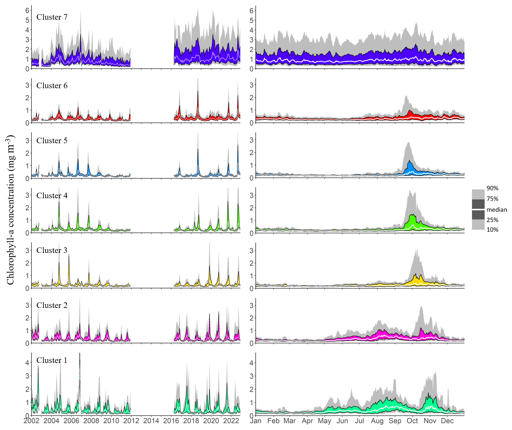
Figure 4 Interannual and seasonal variations in chlorophyll a concentrations, represented by the 10th, 25th, 50th, 75th, and 90th quantiles of all observations within each cluster. The left panel shows interannual variability based on monthly quantiles from 2002 to 2022, while the right panel depicts the seasonal cycle using daily quantiles pooled across the same period.

3.3 Overall Patterns of Change in Surface Chl a

Figure 5 shows maps of overall absolute and relative decadal trends in Chl a concentrations in Lake Tanganyika and the corresponding p-values. A general decrease in Chl a concentrations is observed across most of the lake's surface, except in shallow areas where concentrations remain higher throughout the year. To examine how trends vary with depth, we computed the mean Chl a trend for all pixels within the same depth range, using 10 m depth intervals. The results show positive mean trend values in areas with maximum depths up to 170 m, beyond which the average trends become negative. For subsequent analyses, this depth will serve as the boundary distinguishing the pelagic and deeper coastal zones from the shallower coastal zones of the lake. Negative absolute trends found in deeper regions are small, rarely exceeding −0.05 mg m⁻³ per decade. They are generally statistically significant, as large areas show p-values below 1 %, as seen on panel C. Although the negative trends indicate a slight decrease in Chl a, they are found in regions where average Chl a levels are already very low. When expressed relative to the interannual median Chl a concentrations, these relative trends correspond to rates of change ranging from close to 0 down to −25 % per decade, with an average relative trend of −9 % per decade. The most severe relative trends in deep zones are found in the north basin and in the south of the lake.

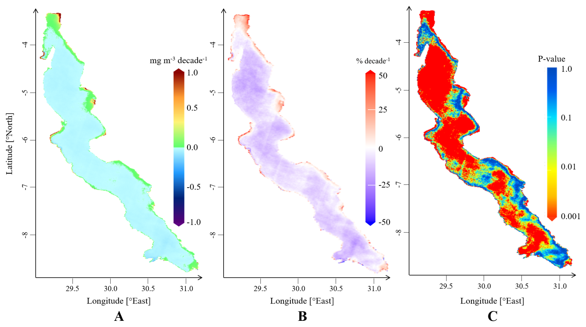
Figure 5 Maps of overall trends in surface Chl a in Lake Tanganyika, depicting absolute trends (A), relative trends computed with respect to pixel-specific median Chl a concentrations (B) and corresponding p-values (C).

Positive trends are observed across 13 % of the lake's surface, mostly in shallower coastal areas that exhibit the highest year-round levels of Chl a. These shallower zones with depth less than 170 m show a wide range of trend values compared to deeper areas, with both lower negative and higher positive absolute trends. Negative relative trends in shallower zones are generally less pronounced than those in deep areas. 25 % of trends in shallow areas exceed 10 % per decade and 10 % exceed 25 % per decade, with some locations reaching increases of up to 50 %. The maximum values are found near Bujumbura, Kigoma and Kalemie, at the estuary of the Malagarasi river and in the Gulf of Burton, where trends values exceed 1 mg m⁻³ per decade.

3.4 Monthly Dynamics of Surface Chl a Trends

Throughout the year, the lake's dynamics reveal a complex pattern of Chl a trends. Figure 6 illustrates monthly relative trends in Chl a concentrations, calculated based on monthly trends divided by the monthly median. Pelagic trends appear to closely align with Chl a seasonality. In the deeper areas of the lake, trends generally shift from predominantly decreasing between February and July to mostly increasing between August and October. From February to April, as Chl a concentrations reach their lowest annual levels, starting in the south and progressing northwards as seen in Fig. 2, negative Chl a trends follow the same south-to-north pattern, extending across all deeper regions of the lake by April. Relative trends show peak negative values of approximately −30 % per decade, as seen in Fig. 6, amounting to absolute trends up to −0.05 mg m⁻³ per decade. Starting in May, trends in deeper zones increase from the south. By August, Chl a trends reach a first positive peak in southern clusters 1, 2, and 3, with relative increases ranging between 10 % and 20 % per decade and up to 30 % per decade in the far south. In contrast, August trends show no statistical significance in the northern deeper areas of the lake. In September, significant positive trends are found in the centre and northern part of the lake, reaching values of up to 50 % per decade in some areas. October is characterized by widespread positive trends in surface Chl a levels, with the highest values observed in the central and southern parts of the lake. From November to January, trend values become less pronounced and less significant, coinciding with the rainy season when the availability of optical data is at its lowest. Contrasting with the seasonality of pelagic Chl a trends, shallow zones exhibit positive Chl a trends throughout the year. These trends remain relatively stable in magnitude.

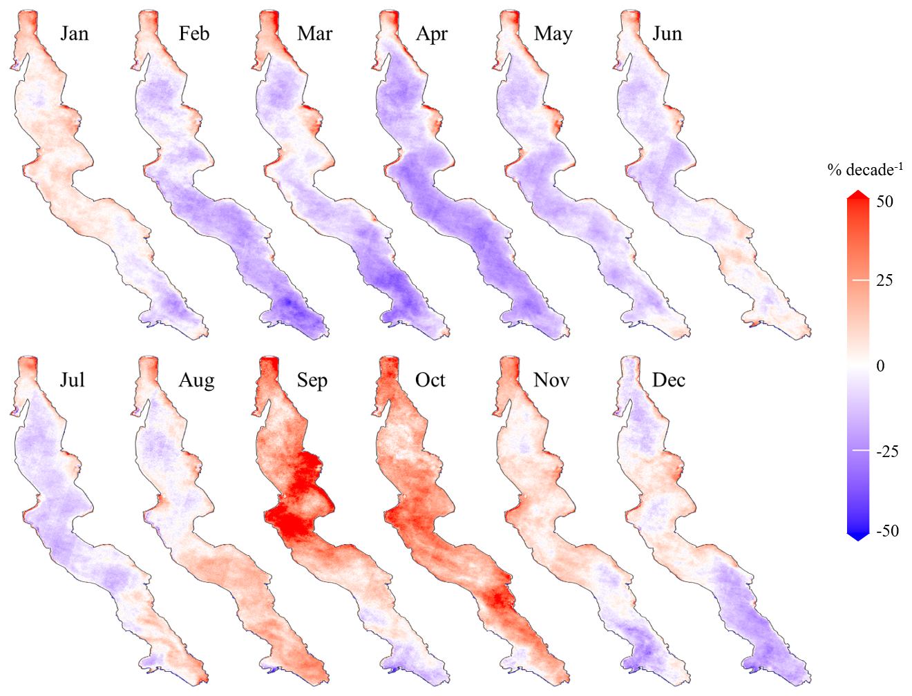
Figure 6 Maps of monthly relative trends in Chl a concentrations in Lake Tanganyika (2002–2022).

3.5 Partition and Shifts in Chlorophyll a Distribution

To evaluate how the yearly distribution of Chl a concentrations has evolved from 2002 to 2022, we analysed trends of yearly quantiles values for each pixel covering Lake Tanganyika. Figure 7 shows spatial median quantile trends by cluster across the yearly statistical distribution of Chl a, with a distinct focus between deeper and shallower regions. Overall, we see that nearly all clusters exhibit slightly positive changes in shallow areas for most of their distribution, with higher trends for the highest quantile values. In deeper zones, most clusters exhibit negative changes for quantiles up to the 75th to 90th percentiles.

More specifically, shallow areas show the steepest increases in cluster 7, while cluster 2 exhibits decreasing values between −5 % and −10 % per decade across most of its distribution, below the 80th quantile. Clusters 1 and 4 display near-zero changes in their lower quantiles while clusters 3, 5 and 6 show modest increases of between 5 % and 15 % per decade. Notably, all clusters exhibit sharp increases in the highest quantiles, ranging from 10 % to 30 % per decade. For trends in deeper areas, clusters 1 to 5 exhibit decreases for all quantiles below the 75th to the 90th percentiles, with values ranging from 0 % to −15 % per decade. In contrast, higher quantiles show sharp increases, ranging from 10 % to 30 % per decade. Cluster 6, located at the northern end of the lake, shows consistent increases around 5 % per decade for the entire distribution below the 90th percentile. For both shallow and deep zones of the lake, this peaks in trends for the highest yearly quantiles could suggest more frequent extreme events, although statistical tests failed to detect any significant changes in the frequency or extent of major bloom events.

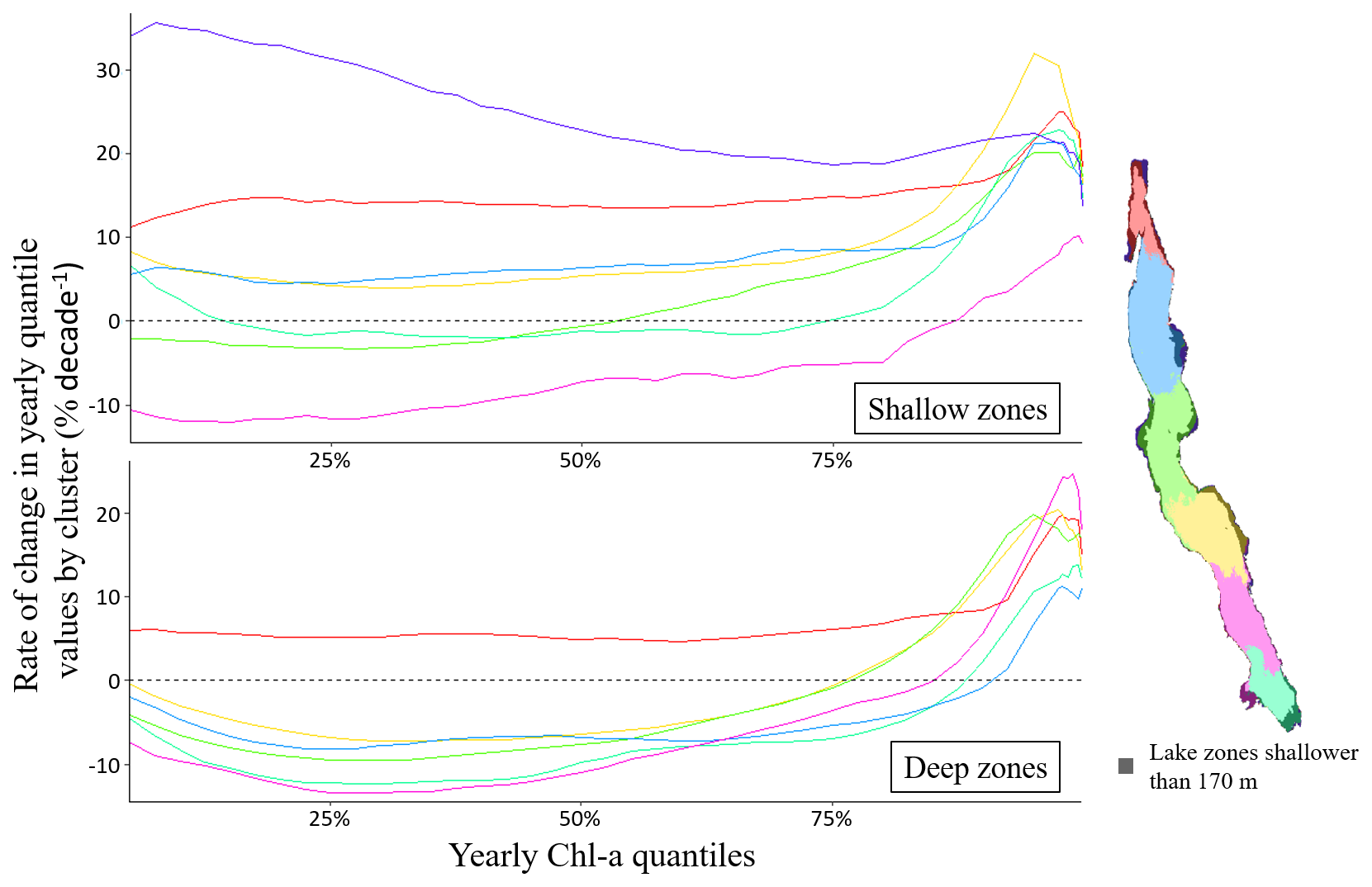
Figure 7 Cluster-specific median rate of change in yearly Chl a quantiles in shallower and deeper zones. The map of the lake shows the areas shallower than 170 m in each cluster.

4 Discussion

The analysis of chlorophyll a (Chl a) seasonality in Lake Tanganyika reveals a highly structured yet dynamic ecosystem, whose spatial and temporal variability cannot be fully captured by field-based observations alone. Satellite remote sensing provides a long-term, lake-wide perspective, allowing Chl a seasonality to be characterized across the entire surface over an unprecedented time span.

In pelagic waters, Chl a closely follows the lake's hydrodynamic cycle, highlighting the dominant influence of wind-driven thermocline dynamics on phytoplankton biomass. While the hydrodynamic framework identifies four seasonal periods, satellite observations suggest a simpler, three-phase biological response. During the dry, windy season, southeasterly winds tilt the thermocline, increasing nutrient availability and triggering phytoplankton blooms, with maximum concentrations appearing first in the south. After the wind reverses, thermocline oscillations propagate blooms from north to south, consistent with previously described upwelling dynamics. Notably, Chl a concentrations during this phase are higher than those reported in earlier studies, suggesting either stronger bloom intensity or improved detection via satellite data. During the late rainy season, weaker winds and a deepening thermocline produce a basin-wide minimum in Chl a. This difference between hydrodynamic cycles and biological response shows how phytoplankton integrate physical forcing into broader, fewer ecological phases.

A key finding of this study is the sharp contrast in Chl a dynamics between shallow (< 170 m) and deep zones. Shallow coastal areas maintain relatively high Chl a year-round, while deeper coastal and pelagic regions experience pronounced seasonal lows, particularly in April. This suggests that depth, rather than distance from the shore alone, is a primary control on phytoplankton biomass. Lake Tanganyika thus comprises two functionally distinct ecosystem types, likely shaped by differences in nutrient availability linked to contrasting water column mixing regimes (Van Bocxlaer et al., 2012).

Earlier spatially explicit studies (Bergamino et al., 2010) focused on annual primary productivity and did not resolve seasonal differences between depth-defined zones. Their identification of high-productivity areas aligns with the shallow, high-Chl a clusters found here, but the seasonal and spatial patterns in shallow zones documented in this study represent a novel contribution. These previously unreported dynamics may have important implications for nutrient cycling, energy flow, and overall ecosystem functioning.

Long-term trends further highlight these depth-dependent differences. Pelagic waters, with pronounced seasonal minima, show declining annual median Chl a, in line with earlier reports of reduced primary productivity due to climate-driven water column stabilization (Bergamino et al., 2010; O'Reilly et al., 2003). At the same time, seasonal trend analysis reveals increasing peak values during the productive season, suggesting that episodic bloom events may be intensifying, as supported by yearly quantile analysis. Shallow coastal zones, in contrast, remain productive year-round and show consistent increases across all seasons. This divergence between average and extreme values underscores the influence of depth-dependent seasonal dynamics on long-term trends and highlights the complex responses of phytoplankton to environmental forcing.

Ecologically, these contrasting trajectories carry important implications. In pelagic waters, declining productivity could reduce energy transfer to higher trophic levels and contribute to lower fish yields. Shallow zones, on the other hand, display dynamic seasonal patterns not previously documented, indicating active processes that could affect nutrient cycling, food web interactions, and ecosystem resilience. Together, these results show that Lake Tanganyika cannot be treated as a uniform system; depth-specific processes must be considered when assessing ecological status and predicting responses to environmental change.

Finally, while satellite data provide a unique lake-wide view, algorithm performance can vary depending on water conditions (e.g., shallow or turbid areas) and the sensor used, and long-term in situ validation remains limited, primarily due to substantial spatial mismatches between point-based field measurements and satellite observations, compounded by sparse coverage, temporal gaps, and methodological variability. These limitations mean that small trends, particularly in pelagic waters, should be interpreted with caution. Nevertheless, the contrasting seasonal and long-term dynamics between deep pelagic and shallow coastal zones are consistently observed across years and spatial clusters, supporting the robustness of the main patterns reported here.

5 Conclusions

This study provides a comprehensive analysis of the seasonality and long-term trends in surface chlorophyll a (Chl a) concentrations across Lake Tanganyika over the past two decades. Our findings highlight the distinct seasonal dynamics of Chl a, driven by the lake's hydrodynamic processes and regional variations in environmental conditions. The analysis confirms that shallow areas exhibit persistently high Chl a concentrations year-round, whereas pelagic regions show strong seasonal variability, with peak productivity following wind-driven mixing events.

The long-term trends reveal a complex duality in the lake's ecological evolution. While deep waters are experiencing a general decline in Chl a concentrations, consistent with previous predictions of reduced primary productivity linked to climate-driven stratification, shallow coastal areas display increasing trends. Notably, in deep areas, while overall concentrations are decreasing, the highest yearly values are showing positive trends, suggesting an increase in extreme Chl a events. These shifts could have cascading effects throughout the lake's trophic network, potentially altering food web dynamics and ecosystem stability.

The observed changes in Chl a underscore the need for further research into the underlying mechanisms driving these changes. A better understanding of how climate variability, nutrient dynamics, and anthropogenic pressures interact to shape the lake's phytoplankton biomass is crucial. Additionally, assessing the cascading effects on zooplankton and fish populations will be essential for developing effective conservation and management strategies. Given the lake's critical role in supporting surrounding populations, continued monitoring efforts using remote sensing and in situ observations are necessary to guide sustainable resource management in the face of ongoing environmental change.