Detecting the resilience of soil moisture dynamics to drought periods as a function of soil type and climatic region

Abrupt changes in climatic conditions and land management can cause permanent shifts in the soil hydraulic response to climatic inputs, impacting soil functions and established soil–climate interactions. To quantify the resilience of soil water content dynamics after abrupt changes in environmental conditions, we present a modelling framework that combines a neural network with seasonal trend analysis (STL). Using data from a series of lysimeters within the TERrestrial ENvironmental Observatories (TERENO)-SOILCan lysimeter network, we identified changes in the response of soil water content after an extremely hot and dry summer in Germany in 2018. The model incorporates meteorological variables decomposed into seasonal and long-term components, together with a categorical indicator of current moisture conditions. It was trained on data from a reference site with a stable soil water content response and applied to lysimeters from multiple origins exposed to contrasting climates. By analysing annual residual patterns – particularly mean bias over time – the soil water content dynamics are classified as being in a “stable”, “resilient”, or “changed” state, reflecting whether the system maintains, recovers, or diverges from its original state. We found that soils preserved their response function to environmental forcing under typical conditions but exhibited changes in hydraulic behaviour when relocated to new environments, even when soil texture remained constant. The proposed method offers a scalable and non-invasive tool for tracking changes in soil water content response to climate change and provides early indicators of changes in essential soil functions and soil health status.

1 Introduction

Soil water content plays a fundamental role in hydrological processes and land–atmosphere interactions, governing the exchange of water and energy at the Earth's surface (Seneviratne et al., 2010; Sun et al., 2025). It regulates key hydrological functions, including infiltration, runoff generation, evapotranspiration, and groundwater recharge. Through these processes, soil water content influences water availability, ecosystem productivity, and climatic conditions across local and global scales (Bogena et al., 2015; Fatichi et al., 2020). Soil water content status and related soil environmental conditions change with short- and long-term atmospheric processes. This response of soil water content to atmospheric conditions, which is defined here as the “soil water content response function”, determines, for example, whether anaerobic conditions are inhibited after heavy rainfall (through fast percolation to deeper soil layers) and whether enough water remains available after dry periods for plant growth, temperature regulation, and chemical reactions. In short, the soil water content response function is an indicator of near-surface hydraulic functioning and land–atmosphere exchange processes, which are relevant for several soil health–related aspects such as infiltration efficiency, surface aeration, and runoff generation. This response function is shaped by soil formation processes and reflects adaptation to the dominant climatic conditions (Kuzyakov and Zamanian, 2019; Sainju et al., 2022). Accordingly, a change in the response function following extreme climatic events is likely to indicate a change in soil health.

At the core of this study is the question of how changes in the soil water content response function, and thus in soil properties and health, can be detected. The standard approach to determine the response function is to apply physically based models, for example, by inverse modelling of soil water content dynamics under varying boundary conditions (Šimůnek et al., 2016). These models require detailed knowledge of soil hydraulic properties and extensive calibration, limiting their generalisation beyond the spatial scale and the local conditions used for calibration (Lehmann et al., 2020; O and Orth, 2021). Additionally, soil hydraulic parameters for physically based models are usually obtained through soil sampling or sensor installation, both of which disturb the soil structure, limiting the feasibility of repeated measurements for long-term time-series analysis. Moreover, these models typically assume static soil characteristics, failing to adequately represent structural changes in soil properties – such as compaction, degradation, or organic matter loss – that can substantially alter hydraulic behaviour over time (Fatichi et al., 2020; Melsen and Guse, 2021; Wankmüller et al., 2024). Most models also neglect or oversimplify the hysteretic nature of the soil water retention curve, as well as seasonal changes in soil hydraulic properties that can substantially alter infiltration, drainage, and plant water availability (Aqel et al., 2024; Hannes et al., 2016; Herbrich and Gerke, 2017). Therefore, we used a non-invasive approach based on neural networks as discussed below.

In recent years, artificial intelligence (AI), particularly neural networks, has emerged as a promising alternative for modelling complex hydrological processes (Reichstein et al., 2019). These data-driven models have demonstrated the ability to learn nonlinear relationships directly from observational datasets without strong reliance on explicit physical equations (Kratzert et al., 2019; Mosavi et al., 2018; Shen et al., 2018). Within soil hydrology, neural networks have been used to characterise hysteretic soil–water behaviour from training data, improving the representation of wetting–drying cycles without explicit hysteresis parameterisation (Aqel et al., 2024). They have also been applied to soil-moisture time-series modelling using Long Short-Term Memory (LSTM) networks with recurrent architectures suited to capture long-range temporal dependencies (Liu et al., 2023; O and Orth, 2021). Across diverse hydro-climatic regimes, LSTMs have been shown to effectively learn nonlinear relationships between climatic inputs and soil water content, often matching or surpassing traditional physically based approaches and demonstrating strong generalisation (Kratzert et al., 2019; Liu et al., 2022, 2023; O and Orth, 2021).

Independent of the chosen modelling approach, these models often ignore the fact that the soil water content response function (i.e., the variations in soil water content following changes in atmospheric conditions) can change over longer time scales. Experimental studies have shown that extreme events such as drought can induce persistent shifts in soil water content dynamics, potentially leading to alternative stable states (see Robinson et al., 2016; Quintana et al., 2023 and the section on illustrative examples in Robinson et al., 2019). Moreover, changes in land use – such as forest conversion to agriculture or bare land – alter soil hydraulic properties, with effects on infiltration, water retention, and saturated hydraulic conductivity (Fu et al., 2021; Robinson et al., 2022). Considering that soil texture (particle-size distribution) is assumed to remain constant at time scales of decades, the changes in the response function are likely related to changes in soil structure and associated hydraulic properties driven by structural reorganisation, wettability effects, root activity, or land-use changes rather than to textural change.

Soil systems are subject to temporal change, yet models are often trained on historical datasets without evaluating whether the system dynamics remain stable throughout the training period (Montanari et al., 2013; Vaze et al., 2010). As a result, models may be applied to prediction settings where underlying soil–climate interactions differ from those on which the model was trained. For example, a recent study comparing different crop models using the TERENO-SOILCan set-up showed that predicting agronomic and environmental variables under different climatic conditions from those represented in the training datasets resulted in significant discrepancies between simulations and observations (Groh et al., 2022). This underscores the critical need to assess whether site-specific representations of soil–water behaviour remain valid over time (Hrachowitz et al., 2013) and highlights the need for more adaptable modelling approaches under evolving environmental conditions (Blöschl et al., 2019; Milly et al., 2008). A recent modelling framework by Jarvis et al. (2024) takes a major conceptual step forward by explicitly representing soil-structure dynamics and their feedback on hydraulic behaviour. However, as the authors emphasize, such process-based models still depend on detailed observational data to constrain temporal changes in structure and hydraulic properties.

To address this gap, the present study introduces a framework based on neural networks and seasonal trend decomposition. This framework is applied to quantify changes in the soil response function following the 2018 summer drought, a Europe-wide extreme event. During this period, total precipitation in central Europe fell to the lowest percentiles relative to the 1976–2005 reference distribution. In Germany, the summer of 2018 was among the warmest on record and had the lowest precipitation since 1881 (Xoplaki et al., 2025). The response of soil water content to this drought will be analysed with a set of lysimeters. As shown in Fig. 1 for one of the study sites, the monthly water deficit (potential evapotranspiration minus precipitation) peaked in summer 2018, indicating a strong drought during this period.

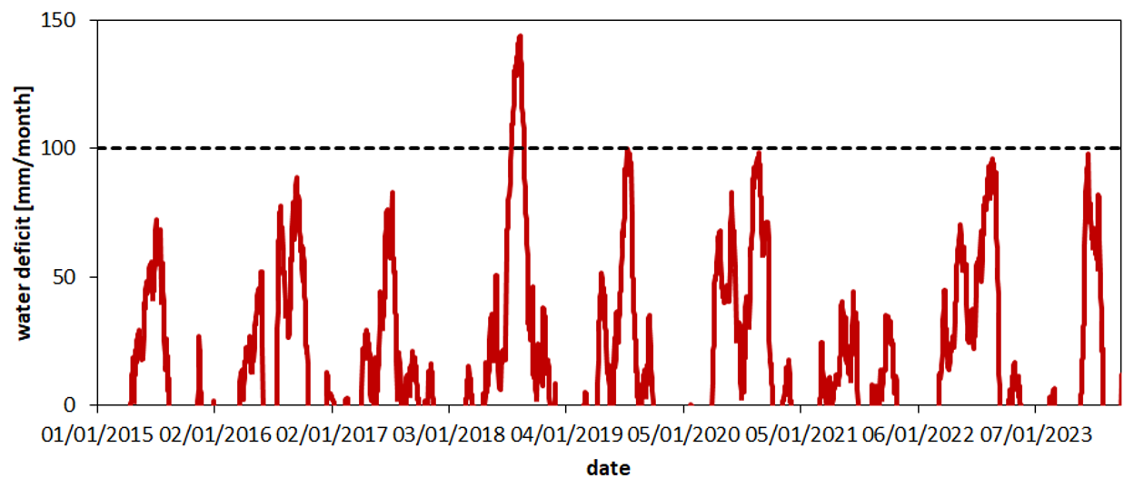
Figure 1 Variations in climatic conditions at Selhausen (SE) are expressed as the difference between potential evapotranspiration (PET) and precipitation (P) accumulated over the preceding 30 d (one month). The extreme summer of 2018 is manifested by a maximum monthly deficit of ∼150 mm. Details on the calculation of PET are provided in Sect. 2.1.1.

Accordingly, the general objective of this study is to introduce a model framework to quantitatively detect changes in the soil water content response function and classify it as “stable”, “resilient”, or “changed”. These terms are used here as operational classes describing the temporal behaviour of the response function, rather than as formal system-level properties or metrics as defined in ecological and complex systems theory. In that framework, resilience is commonly understood as a system property reflecting the capacity to absorb disturbance and recover, including both resistance to perturbation and recovery towards pre-established levels. Stability, in contrast, refers to the tendency of system dynamics to remain close to a reference state or equilibrium (Holling, 1973). In this study, “stable” denotes that a single response function remains valid throughout the entire monitoring period. “Resilient” denotes a temporary deviation from this response function following an extreme event (summer 2018), followed by a return to the pre-event response within the observation window. In the third case, denoted here as “changed”, the response function at the end of the observation period remains distinct from the pre-2018 reference response. Whether such a change represents a persistent transition to an alternative response regime or a transient deviation with delayed recovery cannot be determined based on the available time series.

In principle, it would be possible to develop a quantitative framework to detect changes in the response function exclusively based on experimental time-series data (without modelling), for example, by the application of wavelet analysis (Ehrhardt et al., 2025). In this study, we adopt a predictive modelling approach in which deviations between observed and simulated soil water content over time are used to identify changes in the soil–climate response function. While the model also produces predictions of soil water content, prediction accuracy is not the primary objective; instead, model–data deviations are used to detect temporal drift in soil water response behaviour. The overall level of dynamic agreement is summarized using the Nash–Sutcliffe efficiency, while the detection and classification of changes rely on the temporal evolution of mean bias, as described in Sect. 2.5.

2 Materials and Methods

We developed a data-driven modelling framework that combines time-series decomposition of climatic inputs with a feed-forward neural network to predict the daily soil water content (Fig. 2).

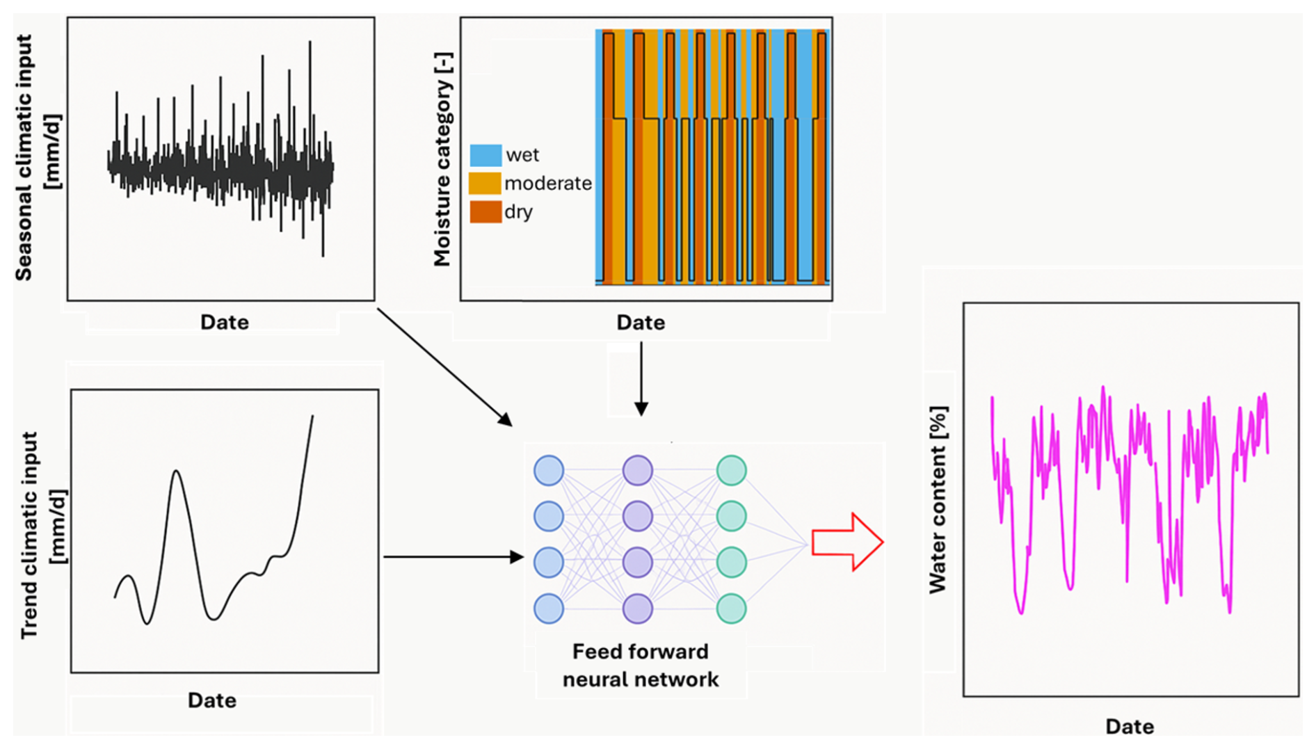
Figure 2 Schematic overview of the modelling framework for daily soil water content prediction. Input features include the analysis of a climatic variable (top left), its long-term trend component (bottom left), and the categorical soil water content state (“wet”, “moderate”, “dry”; top middle). These features, derived from observed data, are used to train a feed-forward neural network (centre), which outputs daily predictions of volumetric water content (right). The model thus captures temporal soil water content dynamics based on structured climate signals and categorical conditions.

The approach explicitly incorporates precipitation (P), potential evapotranspiration (PET), and their difference (climatic water balance) as primary inputs. Each of these climate drivers was decomposed into seasonal variations and long-term trend components using Seasonal-Trend decomposition (STL) and was included as a separate feature in the model (Boergens et al., 2024; Cleveland et al., 1990). The daily climatic water balance (WB) was included to reflect the net difference between P and PET, serving as a proxy for wetting or drying conditions. Positive values indicate potential moisture accumulation (e.g., during rainfall-dominated periods), while negative values reflect high evaporative demand and drying conditions (e.g., during hot, dry spells). Including WB helps the model distinguish between humid periods and dry ones. By providing WB alongside P and PET, the model can learn both the individual and combined effects of precipitation and evaporative demand on soil water content dynamics (Brocca et al., 2010; Uber et al., 2018). For example, it can infer that 10 mm of P during a high-PET summer day (low positive or negative WB) is less likely to increase soil water content than the same P on a cool, low-PET day (high positive WB).

The input features also included a categorical moisture class (type) that reflects the expected current soil water condition (“wet”, “moderate”, “dry”). This design reflects the understanding that changes in climate, such as shifts in rainfall and evaporative demand, substantially affect soil water availability and fluxes (Vereecken et al., 2022). The methodology is detailed in the following sections and consists of six key steps: selecting study sites and datasets collected in contrasting hydro-climatic conditions (Sect. 2.1), preprocessing the data and extracting meaningful signal features including STL (Sect. 2.2), constructing and training a neural network model on a reference dataset (Sect. 2.3), generating soil water content predictions for independent (non-training) sites using the trained model (Sect. 2.4), evaluating the model's performance with statistical metrics (Sect. 2.5), and physical consistency checks (Sect. 2.6).

2.1 Study Sites and Data Selection

2.1.1 The TERENO-SOILCan Lysimeter Network

The study was conducted using lysimeter data from the TERENO-SOILCan lysimeter network in Germany (Pütz et al., 2016) with a focus on two locations: Bad Lauchstädt (BL) and Selhausen (SE) (Fig. 3). These sites were selected for their contrasting climatic regimes and the specific set-up of lysimeters, providing a natural experiment to assess how climate variability influences soil hydrological behaviour across a variety of soils. The TERENO-SOILCan lysimeters were relocated between and within observatories according to a modified space-for-time approach, to expose them to different climates (Groh et al., 2020). This allowed us to compare the ecosystem response of the same soil under different climatic conditions. Selhausen is characterised by a humid, Atlantic-influenced climate (annual precipitation around 720 mm and mean air temperature around 10 °C), whereas Bad Lauchstädt represents a drier, more continental climate (annual precipitation roughly 487 mm and mean air temperature approximately 8.8 °C); both climate descriptions were based on Pütz et al. (2016). Long-term observations confirmed that Bad Lauchstädt experiences significantly lower rainfall and higher evaporative demand than Selhausen, yielding a higher aridity index (ratio of potential evapotranspiration to precipitation) and more pronounced dry spells in the growing season. By including both a wetter site (Selhausen) and a drier site (Bad Lauchstädt), the model was evaluated under distinctly different moisture regimes, which is critical for testing the generality of the approach and distinguishing between climatic and soil type effects. For each lysimeter station (Bad Lauchstädt and Selhausen), 12 lysimeters (1 m² surface area, 1.5 m depth) arranged in a hexagonal configuration with 6 lysimeters around a service well were included in the analysis to monitor soil water content along with meteorological variables. In this study, lysimeters were not used for drainage or storage estimates, but rather as instruments providing long-term, high-resolution time series of soil water content and matric potential under field conditions. The lysimeters contain undisturbed soil columns collected from four different locations (see Fig. 3a), each with three replicates (Pütz et al., 2016) and are managed as arable land under crop rotation. Note that all lysimeters were collected in the field and transported to the lysimeter station (Pütz et al., 2016), such that no differences in packing and boundary effects are expected. While fertilization practices differed regionally until spring 2019, the overall management concept was comparable, ensuring that differences in water dynamics can be attributed to changes in climate and soil rather than management (Pütz et al., 2016).

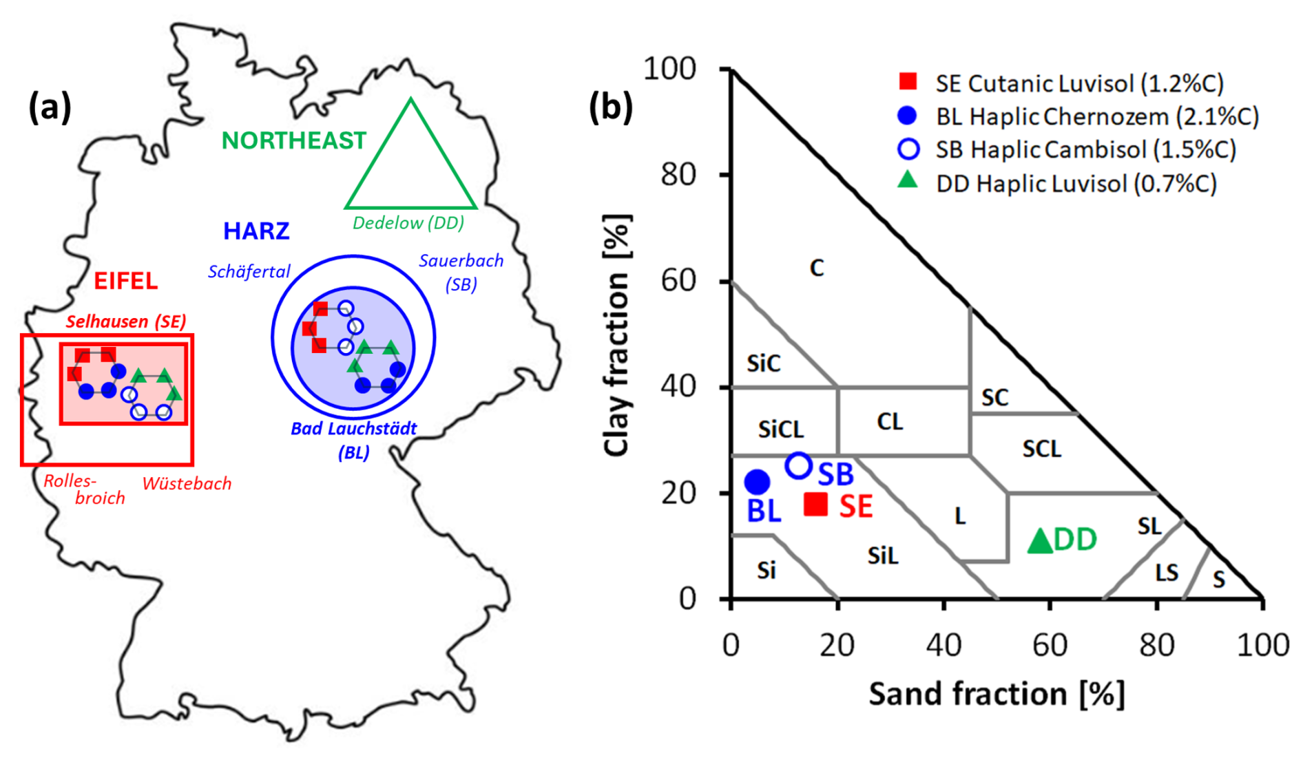
Figure 3 Overview of the study area with site locations, topsoil texture, and soil origin. (a) The TERENO-SOILCan network contains lysimeters from four climatic regions (different symbols and colours in the map). Our analysis focuses on the TERENO-SOILCan sites Selhausen (SE) and Bad Lauchstädt (BL), located in the Eifel/Lower Rhine Valley and Harz/Central German Lowland Observatory of TERENO, respectively, because at both sites lysimeter clusters were built (represented by shaded areas and hexagons), collecting large soil columns from four distinct source regions (i.e., Dedelow (DD), Bad Lauchstädt (BL), Sauerbach (SB), and Selhausen (SE)). (b) The analysed soil horizons (10 cm depth) cover two textural classes, shown in the USDA soil texture triangle, assigned to four different soil types and a range of soil organic carbon contents (SOC) (numbers in the legend).

To investigate the effects of climate on soil water dynamics, daily time series of precipitation (P), potential evapotranspiration (PET), matric potential, and volumetric soil water content (which was used as the target variable) were compiled. Precipitation at Selhausen was measured at the on-site SOILCan weather station, while for Bad Lauchstädt it was taken from the nearest long-term monitoring station operated by the Deutscher Wetterdienst (Leipzig/Halle, ID 2932; DWD Climate Data Centre, 2025). PET was calculated with the FAO-56 Penman–Monteith model (Allen et al., 2006), using measured meteorological variables (air temperature, air pressure, relative humidity, radiation, and wind speed) according to SOILCan protocols (Pütz et al., 2016; Groh et al., 2020). In this context, the reference evapotranspiration (ETo) calculated with the Penman–Monteith model for a clipped grass surface (FAO-56) was used as a proxy for potential evapotranspiration (PET), representing the site-independent atmospheric evaporative demand. Soil matric potential was measured using MPS-1 sensors (Decagon Devices Inc., Pullman, WA, USA), and volumetric soil water content was measured with time-domain reflectometry probes (CS610, Campbell Scientific, North Logan, UT, USA). The observational record spans the period from 2014–2023 and includes measurements taken at a depth of 10 cm (deeper soil layers were not analysed; Pütz et al., 2016).

2.1.2 Definition of Reference Site for Model Framework

For model development, a single lysimeter moved from Dedelow to the Bad Lauchstädt lysimeter station (see Fig. 3a and b) was selected as the training dataset. This lysimeter was chosen due to its stable soil water content dynamics and minimal temporal drift in water retention properties over the observation period (see Fig. 4a). This lysimeter served as the reference dataset for developing the predictive model because it allows the definition of the soil water content response function for seasonal climatic conditions. The 23 remaining lysimeters at the Bad Lauchstädt and Selhausen sites were used as independent test datasets (a contrasting example is shown in Fig. 4b) to evaluate model generalisation and detect potential shifts in soil hydraulic behaviour across sites and years.

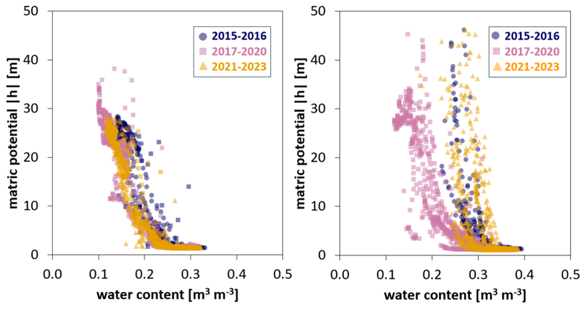
Figure 4 Soil water retention curves using data collected between 2015 and 2023 at 10 cm depth. Matric potential is plotted against volumetric water content, with data colour-coded by period: 2015–2016 (blue), 2017–2020 (green), and 2021–2023 (red). (a) Training lysimeter (moved from Dedelow to Bad Lauchstädt). (b) Test lysimeter (original soil from Selhausen in lysimeter station at Selhausen).

2.2 Data Preprocessing and Feature Engineering

All raw data were aggregated or resampled to a daily time step to support time-series analysis and modelling. Any misaligned or duplicated timestamps were corrected to ensure consistency. Measurements before 2015 were excluded from both sites to allow sensor settlement after installation.

2.2.1 Seasonal-Trend decomposition

To provide the model with structured representations of climate variability, each climatic time series was decomposed into additive components using STL (Seasonal–Trend decomposition based on LOESS, a locally weighted regression method) (Cleveland et al., 1990). STL is a non-parametric method that separates a time series into three interpretable components: a seasonal component representing repeating seasonal patterns (such as wetting and drying cycles), a trend component capturing gradual long-term changes (such as climate shifts), and a residual component containing short-term irregularities and high-frequency noise (Cleveland et al., 1990). This decomposition was applied independently to the P, PET, and WB time series. Only the seasonal and trend components were retained as input features, as they contain meaningful patterns relevant to soil water content dynamics. The residual component, which lacks a systematic structure, was excluded from further analysis. STL was configured with a cycle length of 180 d, representing the semi-annual wet–dry phases at the study sites. A LOESS smoother with a 90 d window was then applied to the de-seasonalized series to extract the trend component. This configuration was chosen to capture gradual, long-term changes in the climatic variables while reducing short-term fluctuations. However, near the ends of the time series, the absence of future values causes the smoothing window to become asymmetric. As a result, the estimated trend becomes more sensitive to recent variability. This limitation does not affect the outcome of the analysis, as both the input features and the target variable (water content) are equally influenced by it. Each of the extracted seasonal and trend components from P, PET, and WB was included as input to the neural network alongside the original raw values. This allowed the model to learn structured seasonal behaviour – such as distinguishing the rising phase of spring wetting up of the soil profile from the declining phase of a summer dry-down – and to account for long-term shifts, such as gradual drying or changes in mean climate conditions.

2.2.2 Wetness classification

In addition to the continuous climate-related features, a categorical input was included to describe the soil moisture condition as either “dry”, “moderate”, or “wet”. These categories were defined using the soil water content time series from the training site, with thresholds based on quantiles of the full distribution. Specifically, values below the 30th percentile were labelled as “dry”, between the 30th and 70th percentiles as “moderate”, and above the 70th percentile as “wet”. These categories were encoded numerically prior to modelling, using values of 30 for “dry”, 20 for “moderate”, and 1 for “wet” (higher values correspond to drier conditions). This encoding allowed the categorical feature to be treated as an ordinal variable and integrated into the neural network input layer alongside the other features. The thresholds were selected to provide clear regime separation while ensuring sufficient observations per class for robust model training.

There were two reasons for including this feature. First, the soil's current moisture condition can strongly influence its response to P and PET (Western and Grayson, 1998). For example, under dry conditions, more water can be absorbed by the soil due to its high storage capacity. In contrast, when soils are already wet or near saturation, infiltration capacity is reduced, and additional rainfall is more likely to result in runoff (Tromp-van Meerveld and McDonnell, 2006; Zehe and Blöschl, 2004). The second reason is the motivation to use remote sensing data in similar follow-up studies, which are not yet accurate enough for modelling purposes but allow a general classification of the wetness status. Because (i) corresponding information on soil matric potential cannot be deduced at larger scales from remote sensing data and (ii) hysteresis in the soil water retention curve may lead to ambiguous thresholds, we focus here on soil water content measurements.

Another aspect of the model framework that must be discussed is the selection of the percentile thresholds. From a soil hydrological point of view, it would make sense that the thresholds defining the three classes “wet”, “moderate”, and “dry” are chosen individually for each lysimeter (a wet clay soil may have very different water content values than a sandy soil). However, from a methodological point of view, we prefer to ensure that the model does not require a long time series to determine quantiles of soil water content data and that it can be applied solely based on the training site's distribution. Accordingly, the same percentile thresholds, derived from the training site, were applied to label daily water content values at the prediction sites. Note that applying the same percentile thresholds for all sites does not affect the detection of changes in the soil water content response function. Very similar results were obtained for a site-specific percentile definition as shown in Sect. S1 in the Supplement. After constructing all the above features, each daily input to the model consisted of (i) raw climate variables (P, PET, and WB), (ii) the STL-derived seasonal and trend components for each variable (six variables), and (iii) the categorical moisture label. All ten features were aligned by date to ensure consistency across inputs. This combination of raw values, decomposed temporal signals, and qualitative soil condition provided the model with a detailed daily representation of both external climatic forcing and internal system state.

2.3 Neural Network Architecture and Training

To model daily volumetric soil water content, a feed-forward neural network was implemented. The architecture consisted of three hidden layers: two dense layers with 12 neurons each using ReLU activation functions (Rectified Linear Units), followed by a batch normalization layer, and a third dense layer with 6 neurons. ReLU was chosen for its ability to introduce non-linearity while maintaining computational efficiency and avoiding vanishing gradient problems during training (Lu et al., 2020; Montesinos López et al., 2022). Batch normalization was applied to stabilize learning by reducing internal covariate shift, which improves convergence speed and training stability (Montesinos López et al., 2022). The output layer consisted of a single neuron with a linear activation function, which is standard for continuous regression tasks such as predicting soil water content.

The network was trained using input features derived from daily observations at the reference lysimeter at the Bad Lauchstädt site, covering the period 2015–2023. Prior to training, all continuous input features were standardized to have a mean of zero and a standard deviation of one using z-score normalization. The standardization parameters (mean and standard deviation) were computed solely from the training dataset and applied unchanged to the validation and test sets at the training site, as well as to the prediction sites, ensuring consistency across all data splits. The target variable, volumetric soil water content, was preserved in its original physical units (m³ m⁻³), allowing for direct interpretation of the model outputs and associated errors in hydrologically meaningful terms. The model was compiled with the Adam optimizer, which adaptively adjusts learning rates and is widely used for its computational efficiency and stable convergence (Kingma and Ba, 2015). Mean squared error (MSE) was used as the loss function due to its sensitivity to large deviations, making it suitable for continuous regression tasks. To monitor generalisation, 30 % of the data were withheld as a validation set and excluded from updating the weights between the nodes during training. The training procedure was initially set to proceed for a maximum of 1000 epochs. To prevent overfitting, an early stopping criterion was implemented based on validation loss. Specifically, training was terminated if no improvement in validation performance was observed over a predefined number of consecutive epochs (patience threshold). The model parameters from the epoch exhibiting the lowest validation loss were retained for final evaluation.

2.4 Testing the Neural Network

After training, the model was applied to the remaining 23 lysimeters across both Selhausen and Bad Lauchstädt, none of which were included in the training phase. All test inputs were processed using the same structure and normalization parameters derived from the training data. As outlined in Sect. 2.1, the experimental setup includes four soil types, each installed with three replicates at both sites (see Fig. 3). While the lysimeters at the Bad Lauchstädt station share the same climatic setting as the training site, the lysimeters at Selhausen represent a more humid region. Accordingly, the raw data and STL-derived seasonal and trend components of the Selhausen climate were used as input for the prediction of soil water content in lysimeters located at Selhausen. This configuration allows for the evaluation of (i) whether the soil water content response function determined for the training site remains valid across different climates and soil types, and (ii) the detection of potential temporal changes in soil hydraulic behaviour. The evaluation and classification procedures are described in the following two Sections.

2.5 Detection of Change in Soil Water Content Response Function Based on Error Metrics

As explained in the introduction, we use error metrics to detect changes in the soil water content response function. While we use the Nash–Sutcliffe efficiency (NSE; see Eq. 5) as a general descriptor of model error, we investigate temporal changes in model performance based on the Mean Bias (MB) that was calculated on an annual basis from 2015–2023. This year-by-year assessment does not rely on predefined change points and enables the detection of gradual or abrupt shifts in model performance directly from the data. MB measures the average signed difference between predicted and observed values, providing an estimate of systematic overestimation or underestimation over time (Moriasi et al., 2007; Liu et al., 2011), and is defined as:

$$\begin{array}{}\text{(1)}& \text{MB}={\displaystyle \frac{\mathrm{1}}{N}}\sum _{i=\mathrm{1}}^N({\widehat{\mathit{\theta }}}_i-{\mathit{\theta }}_i)\end{array}$$

where ${\widehat{\mathit{\theta }}}_i$ is the predicted volumetric water content at day i, θ_i is the corresponding observation, and N defines the number of available observations–prediction pairs. Although the calculation uses daily values, MB was aggregated over yearly intervals to produce a single value per year, capturing annual patterns in prediction bias. Volumetric water content (m³ m⁻³) was multiplied by 100 prior to calculation, and MB is therefore reported in percentage (%). Positive MB values indicate systematic overestimation by the model, while negative values reflect underestimation. The annual assessment of MB allowed us to evaluate whether the soil water content response function remains consistent over time or shows temporal dynamics. Deviations between predicted and observed water content can differ in sign across moisture conditions and event types, such that opposite errors may partially cancel when averaged over a full year. Therefore, mean bias is interpreted as an indicator of long-term temporal drift in model–observation differences, while soil water retention curves are used here (see next section) to verify the physical consistency and direction of detected changes; in cases where retention measurements are not available, robustness of bias trends can alternatively be assessed by repeating the analysis using different temporal aggregation periods.

To classify the soil water content dynamics with respect to the resilience after the extreme summer of 2018, we checked if the deviation of the predictions based on a stable response function (developed using the training data) changed over the years. When the deviation in the first year (2015; i.e., before the drought) is different from the deviation in the year 2023, we consider that the soil water content response function has changed (it is still possible that the response function may recover in the future) and the state of the soil water content dynamics is classified accordingly as being “changed”. When the deviations at the beginning and end are similar, but there was a period between 2018 and 2022 with a different deviation level, we conclude that the soil water content response function changed reversibly over time but recovered within the observation window and the lysimeter is classified as “resilient”. Note that in resilience-related literature, the system response to disturbance is often characterised by the time scale and rate of recovery following perturbation (Scheffer et al., 2009). Here, we do not analyse the recovery period in more detail, but based on the definition of the “resilient” category, recovery must occur within four years.

The soil water content response is considered as “stable” when the deviations remain similar during the entire observation period (i.e., the same response function of soil moisture dynamics to climatic conditions can be used). As a threshold, we chose 1.52 %, which equals the 3-fold of the standard deviation of the nine yearly MB values computed for the training site. The classification of the time series was thus expressed formally as:

$$\begin{array}{}\text{(2)}& {\displaystyle }& {\displaystyle }\text{“changed”:}|{\text{MB}}_{\mathrm{2023}}-{\text{MB}}_{\mathrm{2015}}|>\mathrm{1.52}\mathit{\%}\text{(3)}& {\displaystyle }& {\displaystyle }\begin{array}{rl}{\displaystyle }& {\displaystyle }\text{“resilient”:}|{\text{MB}}_{\mathrm{2023}}-{\text{MB}}_{\mathrm{2015}}|\le \mathrm{1.52}\mathit{\%}\\ {\displaystyle }& {\displaystyle }\wedge |{\text{MB}}_{\mathrm{20}\mathit{\text{xx}}}-{\text{MB}}_{\mathrm{2015}}|>\mathrm{1.52}\mathit{\%}\end{array}\text{(4)}& {\displaystyle }& {\displaystyle }\begin{array}{rl}{\displaystyle }& {\displaystyle }\text{“stable”:}|{\text{MB}}_{\mathrm{2023}}-{\text{MB}}_{\mathrm{2015}}|\le \mathrm{1.52}\mathit{\%}\\ {\displaystyle }& {\displaystyle }\wedge |{\text{MB}}_{\mathrm{20}\mathit{\text{xx}}}-{\text{MB}}_{\mathrm{2015}}|\le \mathrm{1.52}\mathit{\%}\end{array}\end{array}$$

with the logical operator ∧ and the mean bias of a specific year denoted as MB_20xx, which shows the largest difference $|{\text{MB}}_{\text{year}}-{\text{MB}}_{\mathrm{2015}}|$ for the period between 2018 and 2022 (starting with the dry year 2018).

As general information on the different response functions, we calculated the Nash–Sutcliffe efficiency (NSE) coefficient (Moriasi et al., 2007; Nash and Sutcliffe, 1970). The NSE is a standard metric for hydrological model skill, with NSE=1 indicating perfect agreement and NSE≤0, indicating that the model predictions are no better than using the mean of the observations. Mathematically, it is defined as:

$$\begin{array}{}\text{(5)}& \text{NSE}=\mathrm{1}-{\displaystyle \frac{{\sum }_{i=\mathrm{1}}^N({\mathit{\theta }}_i-{\widehat{\mathit{\theta }}}_i{)}^{\mathrm{2}}}{{\sum }_{i=\mathrm{1}}^N({\mathit{\theta }}_i-\stackrel{\mathrm{‾}}{\mathit{\theta }}{)}^{\mathrm{2}}}}\end{array}$$

where ${\widehat{\mathit{\theta }}}_i$ is the predicted volumetric water content at day i, θ_i is the corresponding observed value, $\stackrel{\mathrm{‾}}{\mathit{\theta }}$ is the mean observed volumetric water content over the evaluation period, and N denotes the total number of valid data points used in the calculation. Following Moriasi et al. (2015), model performance was classified as very good for NSE>0.80, good for $\mathrm{0.70}<\text{NSE}\le \mathrm{0.80}$, satisfactory for $\mathrm{0.50}<\text{NSE}\le \mathrm{0.70}$, and unsatisfactory for NSE≤0.50.

In this study, NSE is used to summarize the overall agreement between simulated and observed soil water dynamics, whereas the identification and classification of temporal changes in the soil water content response function rely exclusively on the annual evolution of mean bias. Lower NSE values were interpreted as reduced dynamic agreement between the tested lysimeter and the reference soil–climate response used for training, without implying a specific mechanism of change.

2.6 Interpretation of Change in Response Function in Soil Physical Terms

The dynamics of MB (see above) were also used to assess changes in soil water retention curves (SWRCs), which were plotted for each test lysimeter on a yearly basis. As stated in Eq. (1), a positive MB value corresponds to measured water content values that are smaller than the predictions. Because the predictions are based on the model trained for a specific lysimeter, we expect that, for a positive MB, the water content for the same environmental conditions (as manifested in the matric potential) is smaller in the test lysimeter compared to the lysimeter used for training (SWRC is shifted to the left). Similarly, a consistently negative MB suggests that the test site may retain more water at a given matric potential than the training site, and that the SWRC is likely shifted to the right. For a “resilient” soil, the soil water retention curve shifts back close to the original position at the end of the observation period. Finally, for a soil with a `changed' response function, the water retention curve drifts over time, but without returning to its original position. In some cases, the temporal evolution of MB may not exactly follow the apparent shift of the SWRC, as additional vertical or slope changes could occur due to variations in porosity or pore-size distribution. These effects cannot be identified within the current framework but may contribute to deviations between MB dynamics and the apparent SWRC shift. To further support the SWRC-based interpretation, a quantitative analysis of soil water retention curve evolution based on the concept of integral mean water content is provided in the Supplementary Material.

3 Results

Following the methodological framework described in Sects. 2.3–2.6, we present the model predictions across the test lysimeters to assess the resilience of the soil water content response function for the different lysimeters. We organise the section in four sections according to the four different origins of the soil in the lysimeters (see Fig. 3b) to discuss effects of soil origin and climatic conditions on the response function. In the last section (Sect. 3.5), the results are summarized to allow direct comparison of all 24 lysimeters. Note that all model results presented below are based on the soil water content classification (“wet”, “moderate”, “dry”) as deduced from the lysimeter used for model training. The corresponding figures using a site-specific classification for each lysimeter are shown in Figs. S4–S7 in the Supplement.

3.1 Lysimeters with same soil as used in model training (Dedelow soils)

The neural network was trained to capture the soil water content response function of one lysimeter with sandy loam topsoil (Luvisol) extracted from Dedelow and translocated to the dry climatic region in Bad Lauchstädt (see Fig. S1 in the Supplement). The NSE of the training and validation for that specific lysimeter was very high, with a value of 0.91, indicating good model performance. The application of this response function to the other two lysimeters from Dedelow that were translocated to Bad Lauchstädt resulted in relatively high NSE values (0.79 and 0.84), but the response in summer 2018, characterised by lower soil water content, was not captured accurately (Fig. 5a). More specifically, the time series showed that predictions and observations matched closely in 2015, while after the dry summer of 2018 the model systematically overestimated water content in 2019 and 2020, before the agreement improved again towards the end of the period.

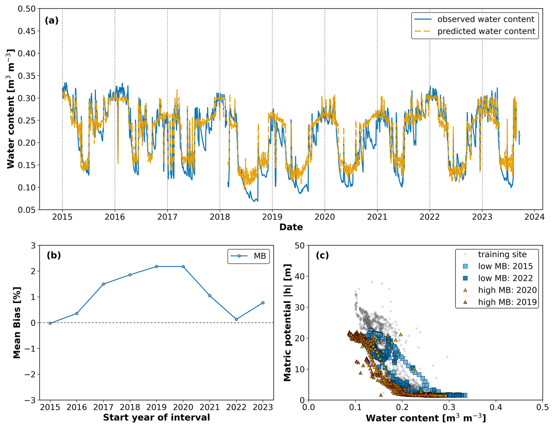
Figure 5 Analysis of soil water content dynamics (2015–2023) for a Dedelow-origin lysimeter tested at Bad Lauchstädt. Panel (a) shows the time series of observed (blue) and predicted (orange) water content, with close agreement in 2015, clear overestimation in 2019–2020 (predictions above observations), and improved agreement again towards the end of the period. Panel (b) presents the temporal evolution of mean bias (MB), remaining near zero until 2017, increasing to about 2 %–3 % in 2019–2020, and decreasing again to approximately zero in 2022. Such soil water content response was classified as “resilient”. Panel (c) displays soil water retention curves from the training site (grey) and from selected years representing different MB conditions, with low-MB years (2015, 2022) and high-MB years (2019, 2020). The curves are close to the training site in 2015, show a shift to lower water contents in 2019–2020, and in 2022 return to the training site data.

These changes are reflected in the MB trend development (Fig. 5b), with values increasing from near zero in 2015 to about 2 %–3 % in 2019–2020 and then decreasing again towards 2022. The retention curves confirm this interpretation (Fig. 5c). The year with low MB (2015) produced a SWRC close to the measured curve of the training site; the years with high MB (2019–2020) were shifted towards lower water contents, and the later year with reduced MB (2022) returned to the measured SWRC of the training site. Taken together, the time series, MB trend, and SWRCs show that the soil response was disturbed after 2018 but later recovered, which classifies this lysimeter as “resilient”. The same finding holds for the simulations of the lysimeters translocated to Selhausen (less dry climate) with high NSE between 0.80 and 0.82. This indicates that for the coarse-textured soil included in this study (i) the effect of changing climatic conditions was rather small (very good NSE classification for both sites), but (ii) that these coarse-textured topsoils do not show identical responses to the extreme year, as each lysimeter reacts slightly differently, which may indicate small differences in hydraulic properties.

3.2 Lysimeters with soils formed under the same climate as the one used in model training (Bad Lauchstädt soil)

The lysimeters filled with soil from Bad Lauchstädt (Chernozem) were formed under the climatic conditions used for fitting the response function. In the case of a dominant effect of climate on the soil water content response function, we could expect similar results as for the training lysimeter. For the soil remaining at the original site (Bad Lauchstädt), the model performance was very good (0.88–0.89). As shown for example in Fig. 6a, the fit between observed and predicted water content was consistently close, with a tendency to slightly underestimate in the early years and to mildly overestimate after 2018, particularly in 2019–2020, before the agreement improved again in later years. This is also manifested in the MB values that increased from slightly negative values in 2015 to about +1.5 % in 2019, before decreasing again towards zero (Fig. 6b). The plotted SWRCs support this interpretation (Fig. 6c), with low MB years (2015 and 2016) showing a slight shift towards higher water contents relative to the measured SWRC of the training site, and high-MB years (2019 and 2020) displaying a modest shift towards lower water contents. Accordingly, the state of the soil water content dynamics was classified as “resilient”.

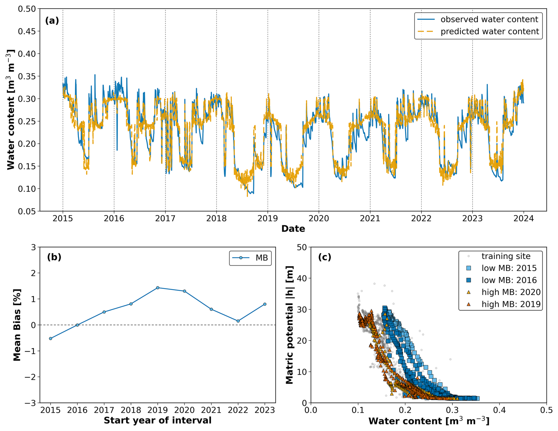
Figure 6 Analysis of soil water content dynamics (2015–2023) for a Bad Lauchstädt-origin soil lysimeter tested at Bad Lauchstädt. (a) Comparison of measured (blue) and simulated (orange) daily water content values, showing high agreement in the early years and temporary overestimation in 2019–2020. (b) Mean Bias (MB) started slightly negative in 2015, increased to about +1.5 % in 2019, and then decreased again towards 2022. (c) Soil water retention curves (SWRCs) from the training site (grey) and from the same replicate for selected years with low MB (2015, 2016) and high MB (2019, 2020) show close agreement in the early years and a shift to lower water contents in 2019–2020.

For the lysimeters transported from Bad Lauchstädt to Selhausen, the performance was more variable (NSE ranging from 0.50–0.84), corresponding to classifications ranging from satisfactory to very good, reflecting the stronger effect of the wetter climate. None of the three lysimeters that stayed in Bad Lauchstädt were classified as “changed”, but two out of three showed a systematic shift and were classified as “changed” when translocated to Selhausen (see Table 1). In short, these examples show that the Bad Lauchstädt soil remained resilient under its original climatic conditions at Bad Lauchstädt but changed when exposed to the wetter climatic conditions at Selhausen.

3.3 Lysimeters with soils formed under a similar climate to the one used in model training (Sauerbach soil)

The findings are similar for the silt loam (Cambisol) from Sauerbach that was formed under climatic conditions similar to those in Bad Lauchstädt. As in the case of the soil from Bad Lauchstädt, soils from Sauerbach show higher NSE values when translocated to Bad Lauchstädt (0.81–0.88, very good) compared to those transferred to the wetter climate in Selhausen (0.74–0.79, good). This reflects that the soil water content response function in the drier climate is not the same as in the wetter climate. In one illustrative case, the observed water content initially showed wetter dynamics than predicted, but gradually converged towards the model predictions by 2023, indicating a possible adjustment in soil hydraulic response over time (Fig. 7a).

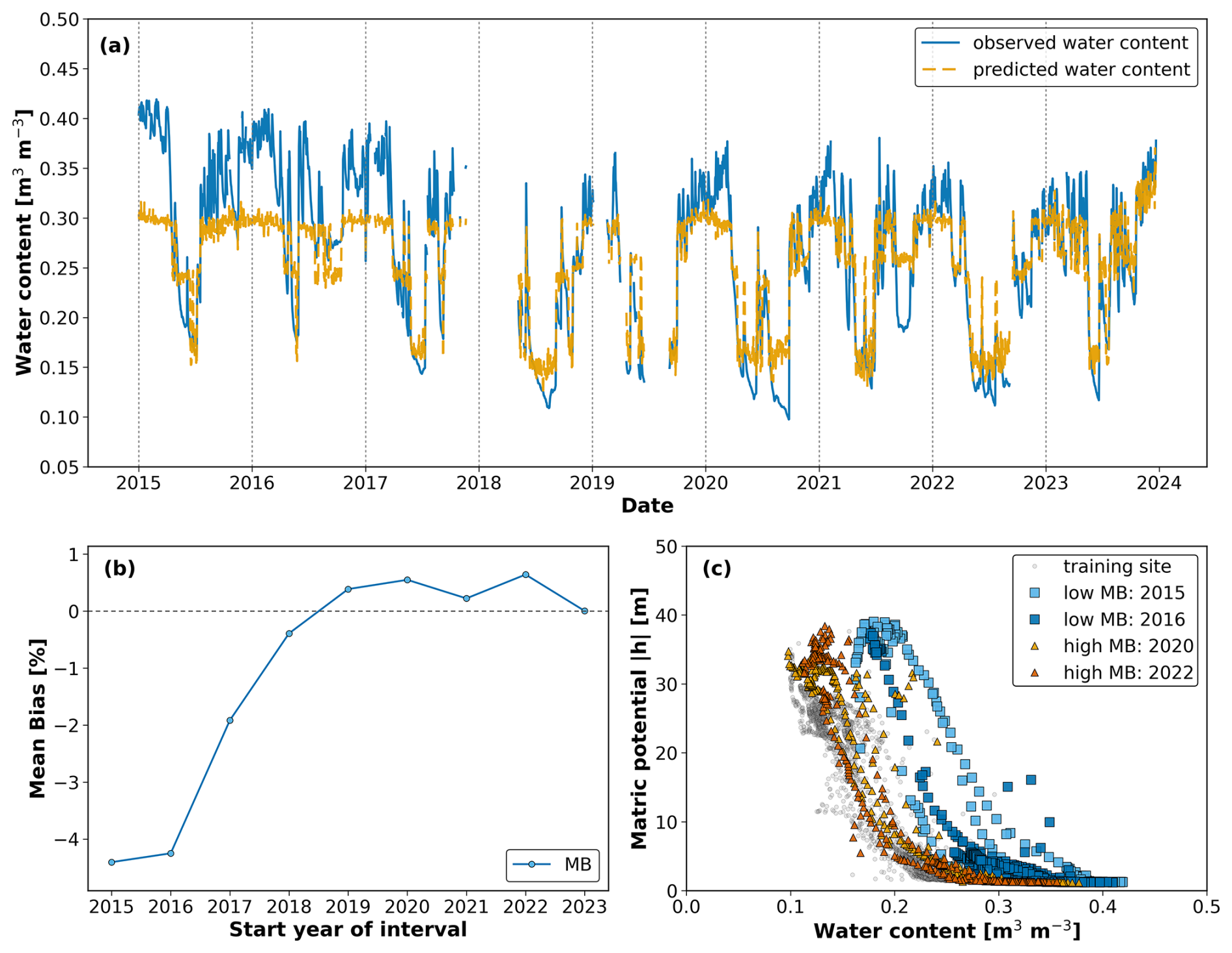
Figure 7 Analysis of soil water content dynamics (2015–2023) for Sauerbach-origin lysimeter relocated to Selhausen (a) Comparison of observed and predicted daily volumetric water content (NSE=0.74); Ater initial underestimation by the model, the observed and predicted values gradually converged, indicating a possible adjustment in soil hydraulic behaviour over time. (b) Temporal evolution of the mean bias (MB), which increased from about −5 % in 2015 to values close to zero by 2019–2023, consistent with the improved match between observed and predicted values shown in panel (a). (c) Soil water retention curves (SWRCs) from the training site (grey) and from selected years with low MB (2015, 2016) and high MB (2020, 2022) illustrate the same trend, with early years showing higher water contents at a given matric potential and later years shifting towards the training curve.

This development is also evident in the MB values (Fig. 7b), which started strongly negative (−5 %) in 2015–2016 and steadily increased towards values close to zero by 2023, indicating a progressive reduction in underestimation. The corresponding SWRCs (Fig. 7c) confirm this trend, with curves from early years (2015, 2016) showing higher water contents at a given matric potential compared to the measured SWRC of the training site, while later years (2021, 2023) shifted closer to the reference, suggesting a gradual adjustment of hydraulic behaviour. In the case of soils from Sauerbach, there was a difference in the quantification of resilience with respect to the classification of the soil water content used as an input variable: with the classification based on the training lysimeter (with sandy loam in the topsoil), the soil water content dynamics were classified as “changed” for all six lysimeters. However, using the classification based on the soil water content statistics obtained for each lysimeter individually (see Fig. S6 in the Supplement), the high water contents at the beginning were better captured, and only one lysimeter out of three was classified as “changed”. Independent of the water content classification, all lysimeters translocated to Selhausen were classified as “changed”, exhibiting the strongest response to relocation among all soils.

3.4 Lysimeters with soils formed under a different climate compared to the one used in model training (Selhausen)

Finally, we discuss the Selhausen silt loam (Luvisol), which was formed under climatic conditions that were not used in the training of the neural network. The model performance was better for the replicates translocated to the drier Bad Lauchstädt climate ($\text{NSE}=\mathrm{0.86}-\mathrm{0.92}$, very good), compared to slightly lower performance at their site of origin under humid Atlantic conditions (0.76–0.86, good to very good). The classification with respect to resilience helps to explain this, since Selhausen soils at their origin were mainly assigned to “stable” or “resilient” categories (see Table 1), while the same soils translocated to Bad Lauchstädt showed a more variable pattern. This indicates that the lower NSE at Selhausen does not represent a misfit of the model but reflects that the soils follow their own stable soil water content response function. One replicate at Selhausen (NSE=0.85) reproduced the seasonal dynamics well, although differences between observed and predicted values remained visible in the wet season across several years (Fig. 8a). The MB shifted from negative values in the first years towards zero after 2019. Note that an MB value of 0 does not mean that deviations disappeared, but that errors in wetter and drier phases compensated each other (Fig. 8b). The SWRCs were generally close to the training reference, but in later years, small deviations appeared mainly at the saturated end (Fig. 8c). Overall, these changes remained below the assumed threshold, supporting the classification of the soil water content dynamics as “stable”.

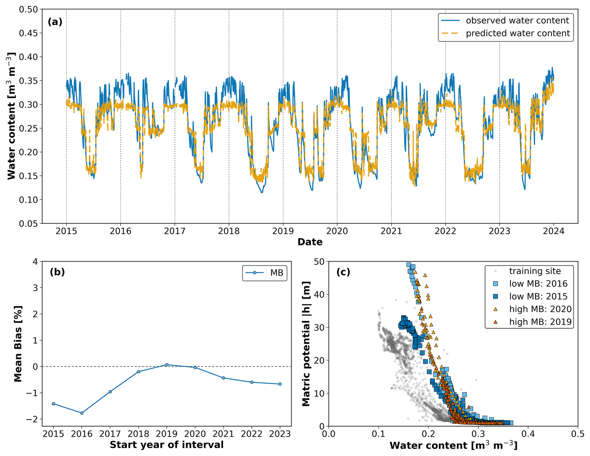
Figure 8 Soil water content dynamics (2015–2023) for a Selhausen-origin lysimeter tested at Selhausen. (a) Observed (blue) and predicted (orange) water content shows fair agreement, with underestimation of water contents in the wet season. (b) Mean Bias (MB) fluctuated from negative values in the early years to values close to zero after 2019, but these variations remained below the threshold for change. (c) Soil water retention curves (SWRCs) from the training site (grey) and from selected years with low MB (2015, 2016) and higher MB (2019, 2020) reflect these minor variations, with the 2019 curve showing the strongest deviation yet remaining close to the training reference, consistent with the stable classification. The apparent cutoff at the wet end in (a) arises from the use of absolute rather than normalized values during training, as discussed in Sect. S1.

3.5 Comparison of all lysimeters

The comparison of the soil water content dynamics of all lysimeters indicates that contrasting climatic conditions between sites – particularly between the continental Bad Lauchstädt and Atlantic-influenced Selhausen – can significantly alter the hydraulic response of the soil, even when texture remains constant. In general, prediction performance at Selhausen was lower, likely because the model was trained under the drier climate of Bad Lauchstädt and therefore failed to fully capture the soil–water interactions emerging under wetter conditions (Fig. 9). The broader NSE range observed at the Selhausen location further suggests increased variability in hydraulic response among replicates.

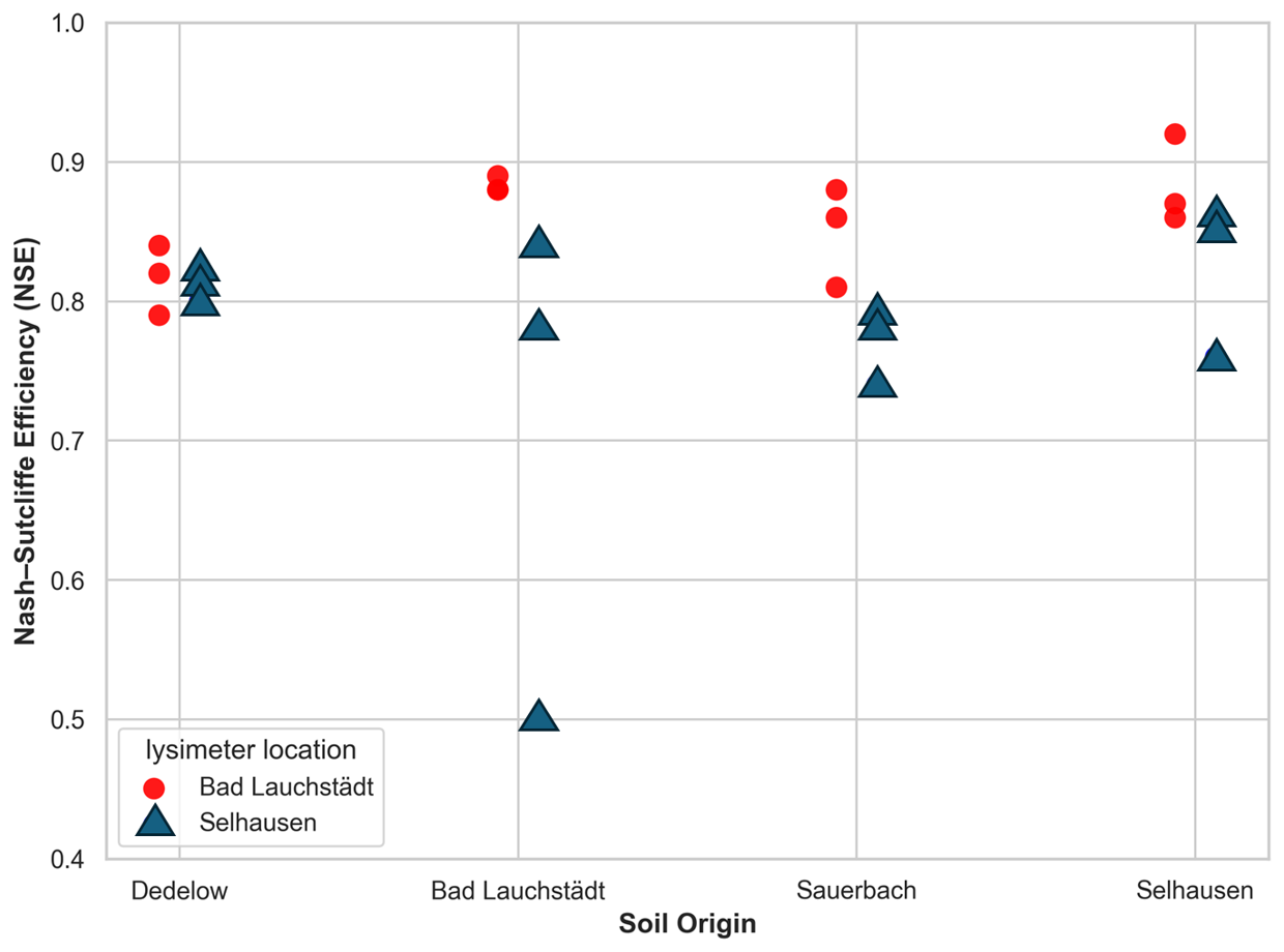
Figure 9 Spread of Nash–Sutcliffe efficiency (NSE) values across different soil origins and test locations. Each symbol represents one lysimeter from a given origin (x axis) evaluated at Bad Lauchstädt or Selhausen (indicated by colour). The results highlight the influence of climate–soil interactions on model performance. Notably, Bad Lauchstädt-origin soils exhibited strong performance at their origin but a wider and lower range when tested at Selhausen, indicating increased variability in soil hydraulic behaviour and divergence in soil–climate response.

With respect to resilience of the soil water content response function, we show the temporal evolution of the mean bias for all lysimeters in Fig. 10 and summarize the results in Table 1. In Table 1 we include the general classification type (“stable”, “resilient” and “changed”) and calculate the average of three lysimeters (same material and same location) for (i) the drift in mean bias value between the year 2015 and 2023 and (ii) the maximum deviation from 2015 for the years between 2018 and 2022. The table shows that deviations from a “stable” or “resilient” response function mainly occur when soils from Dedelow, Bad Lauchstädt, and Sauerbach were translocated to Selhausen. Only in the case of the soil from Selhausen, the response function remains “stable”. It seems that the soil material “trained over decades” to the wetter climate in Selhausen adapts better to the extreme summer 2018.

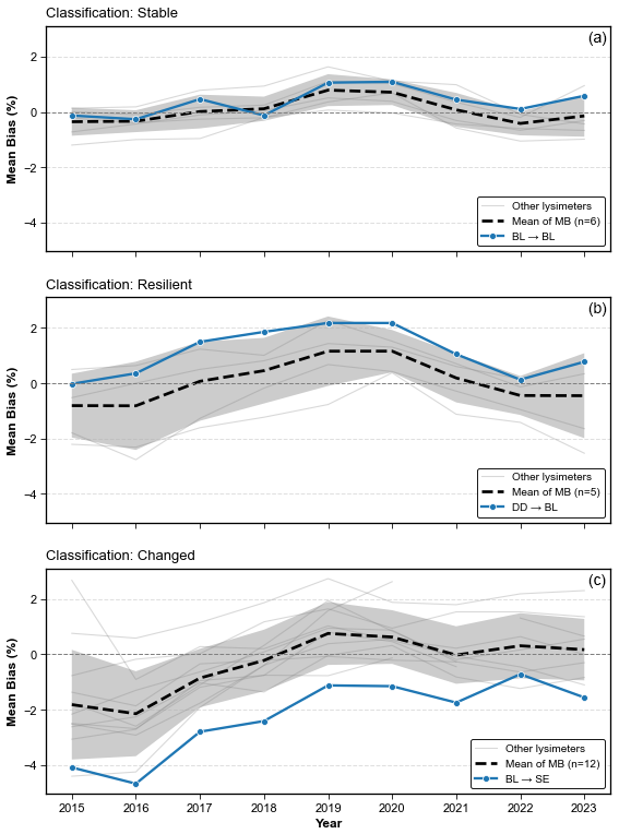
Figure 10 Temporal evolution of Mean Bias (MB) for three representative lysimeter replicates, each classified into one of three soil hydraulic response categories: (a) “stable”, (b) “resilient”, and (c) “changed”. Thick dashed lines indicate the mean of the MB trend across all lysimeters within each classification group, with sample size (n) specified in the legend. Shaded areas represent ±1 standard deviation. Thin grey lines show individual MB trajectories of the remaining lysimeters in each group. Highlighted blue lines depict selected replicates originating from and/or tested at distinct sites: (a) BL → BL (soil material from Bad Lauchstädt tested at its origin), (b) DD → BL (soil material from Dedelow tested at Bad Lauchstädt), and (c) BL → SE (soil material from Bad Lauchstädt tested at Selhausen). These examples illustrate contrasting temporal patterns in hydraulic response, ranging from sustained stability to progressive divergence from the trained site dynamics.

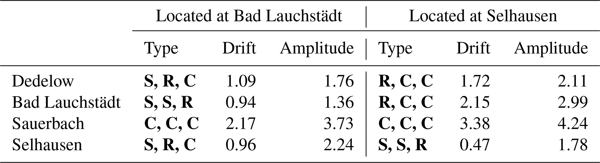
Table 1 Resilience of soil water content response function for the four soil materials translocated to Bad Lauchstädt and Selhausen. The “type” describes the class of response function of the individual lysimeters (S for “stable”, R for “resilient” and C for “changed”). The “drift” is the average value $|{\text{MB}}_{\mathrm{2023}}-{\text{MB}}_{\mathrm{2015}}|$ of the three lysimeters with the difference in Mean Bias (MB) between years 2023 and 2015. The “amplitude” is the maximum difference of the Mean Bias between the first year (2015) and the years between 2018 and 2022 (denoted as year 20xx).

4 Discussion

The results presented in Sect. 3 demonstrate that the model can reproduce soil water content dynamics reliably under stable conditions (as indicated by high NSE values), but it exhibits limitations when soils undergo persistent changes in hydraulic behaviour or are exposed to a different climate. Several soils showed a shift in the wet range, indicating that differences in soil water content response cannot be explained by texture alone but reflect the combined effects of climatic conditions and structural evolution. Based on these findings, the following discussion evaluates how assumptions of static hydraulic behaviour and the response function affect model performance, examines the role of NSE and MB in identifying evolving system dynamics, and reflects on the broader implications for long-term modelling and soil water content monitoring.

4.1 Soil–Climate Interactions as Drivers of Hydraulic Response Function

The predictive success of data-driven models depends not only on the physical properties of soils but also on the climatic context in which those properties developed and continue to function. The present study shows that soils exhibit the most consistent replicate behaviour when evaluated under climate conditions similar to those of their origin, where gradual climatic changes over time have allowed their structure to adjust naturally. When exposed to faster or contrasting climatic shifts, as in translocated settings, the soil response becomes less predictable and less stable. This is demonstrated in Table S1 in the Supplement, which lists the average trends (difference in MB between 2023 and 2015) and amplitudes (difference in MB between 2015 and the dry years) for three lysimeter replicates. Only for the three lysimeters at the original locations (Bad Lauchstädt or Selhausen) were both drift and amplitude below the stability threshold of 1.52 % and could be classified as “stable” as a group of lysimeters.

This suggests that the function of the soil system cannot be meaningfully decoupled from its climatic history. Soils may develop pore arrangements, aggregation patterns and, as a consequence, soil water retention characteristics that reflect long-term adaptation to local hydrological regimes. When these soils are translocated to environments with contrasting precipitation and atmospheric demand, their hydraulic response can shift in ways that are not captured by static texture-based estimates of soil hydraulic properties. Alternative pore-scale processes, including slowly reversible swell–shrink behaviour and non-equilibrium preferential flow, may also contribute to the observed shifts in apparent SWRC behaviour. Recent large-scale analyses have demonstrated statistically significant impacts of climatic factors on soil pore space organisation and laboratory-measured retention characteristics (Hirmas et al., 2018; Klöffel et al., 2024), providing independent support for the plausibility of climate-driven modification of soil hydraulic response.

Such context-dependent behaviour highlights the limitation of the common assumption that soils with the same texture will show comparable retention across regions, an assumption often made in the absence of better descriptors. While laboratory-measured SWRCs show strong and well-established correlations with texture across climatic gradients, particularly in the dry range, experimental evidence collected under natural field conditions indicates that this simplified description does not always hold (Hannes et al., 2016; Robinson et al., 2016; Aqel et al., 2024). In our case, even soils with similar textural composition exhibited different levels of model agreement depending on climate, highlighting that physical similarity (e.g., soil texture) does not guarantee functional equivalence in retention. For example, Selhausen-origin soils achieved higher NSE values when translocated to Bad Lauchstädt, likely because the model was trained under similar dry climatic conditions. However, classification results showed that these soils retained greater stability at their origin, suggesting that predictive success under familiar climatic forcing does not necessarily imply hydraulic consistency. After the 2018 drought, the Selhausen soils translocated to Bad Lauchstädt converged towards similar dynamics across replicates, with MB stabilizing close to zero, indicating that their response functions adjusted consistently to the drier climate (see Fig. S2 in the Supplement). However, a clear carry-over effect was observed: soil water in the upper 10 cm was not fully replenished during the wet phase of autumn and winter 2019 and only reached comparable, though slightly lower, values in winter 2020. A comparable multi-year legacy across the full soil column was reported in the TERENO-SOILCan lysimeter network by Groh et al. (2020).

All mentioned points underscore the importance of including a very broad range of climatic forcing in the assessment of soil model transferability, as demonstrated by Groh et al. (2022). Our results also suggest that future efforts to generalise hydrological models should consider training under a range of climatic conditions to capture the full expression of soil–climate interactions, rather than relying on a single static representation. From a process-based perspective, these findings reflect that climate does not simply modulate soil water content inputs but actively shapes the retention and release behaviour of the soil pore network by driving changes in soil hydraulic response. While management practices across sites were similar, minor differences in tillage and fertilization cannot be completely excluded and may have influenced soil structure and water retention. In addition, monitoring of soil organic matter over time would be useful to link changes in the response function and structure-related soil hydraulic properties to biological processes. Another mechanism that could result in structural changes is swelling and shrinking of the soils with considerable clay content (three soils with ∼20 % clay). Nonetheless, the dominant control remains climatic forcing, which makes this consideration particularly relevant for climate-change experiments: models calibrated under past climatic conditions may not remain valid under the rapid climatic shifts projected for the coming decades. Neglecting this evolving soil–climate feedback could lead to substantial underestimation of future changes in soil hydraulic behaviour and associated ecosystem responses.

4.2 High Predictive Performance Can Mask System Evolution

Although several lysimeters achieved high predictive performance as expressed by high NSE values (Fig. 9), systematic trends in MB suggest that the underlying retention behaviour and soil water content response function may have shifted (Fig. 10 and Table 1). This was most apparent in Dedelow soils translocated to Bad Lauchstädt, where the model maintained high NSE values, but the MB increased across years (see Fig. S3 in the Supplement). The corresponding shifts in the soil water retention curves confirmed a gradual change in how the soil retained water, despite the model continuing to predict moisture levels accurately.

This suggests that local changes in hydraulic behaviour can occur without immediate deterioration in model fit. The predictive framework remained effective in capturing the general moisture dynamics, but the relationship between matric potential and water content was no longer consistent with that observed during training. These findings highlight that high model accuracy does not guarantee stability in soil hydraulic behaviour, particularly under changing environmental conditions. Identifying such divergence early is critical for maintaining reliable predictions in long-term monitoring.

4.3 Implications for Monitoring, Remote Sensing, and Soil Health

The classification outcomes across all lysimeters highlight the role of site memory and hydraulic resilience in maintaining soil water response under climatic stress. Soils assessed at their origin were more frequently classified as “stable” or “resilient” (e.g., Selhausen at Selhausen), while those translocated to different locations were more likely to be classified as “changed” (e.g., Sauerbach at Bad Lauchstädt). As stated in the Materials and Methods section, this classification as “changed” is affected by the length of the observation window and does not allow for a definitive decision between a persistent change to a new response function and a manifestation of a slow recovery rate. Regardless of future developments, these patterns indicate that soil hydraulic behaviour shaped by long-term climatic adaptation may change when soils are exposed to new environmental conditions. The presented methods allow the detection of emerging shifts in soil hydraulic behaviour that may be relevant for soil health assessment and could serve as indicators of deteriorating soil health status.

This has direct implications for long-term monitoring and remote sensing. Our model framework, which avoids reliance on matric potential data and instead uses moisture state categories and decomposed climatic features, is compatible with satellite-derived products. As remote sensing missions increasingly provide continuous global soil water content estimates, the proposed framework could be adapted for large-scale assessment of soil system stability. Furthermore, under scenarios of future climate change, where shifts in precipitation patterns and evaporative demand are expected, data-driven models trained on historical data may become progressively outdated. The presented residual-based approach (quantifying MB) enables early detection of such divergence, offering a method for identifying when model retraining or reparameterisation is needed to maintain predictive reliability under non-stationary conditions.

5 Summary and Conclusions

Temporal variations in topsoil water content control near-surface hydraulic conditions, infiltration, evaporation, and gas exchange, thereby shaping soil water dynamics and physical soil functioning. Reliable information about soil water content dynamics in response to atmospheric conditions is thus essential for detecting and mitigating critical changes in soil hydraulic behaviour. This response depends on soil hydraulic properties that are traditionally characterised by a time-invariant and unambiguous relationship between matric potential, water content, and hydraulic conductivity as deduced from small-scale lab experiments. In this study, we developed and applied a feed-forward neural network combined with seasonal trend analysis of climatic time series to quantify the soil water content response function after an extreme drought in the summer of 2018 in Germany. By analysing the time series of topsoil water content measured at two lysimeter stations of the TERENO-SOILCan network, we summarize the conclusions on the soil water content response function as follows:

• 50 % of the lysimeters showed changes in soil water content dynamics after the dry summer of 2018 without recovery until 2023.

• The remaining lysimeters showed resilient behaviour, and the soil water content response function was not permanently changed.

• Changes in the soil water content response function were manifested as (i) temporal trends in prediction error (mean bias) and (ii) shifts in the soil water retention function.

• The soil water content response function is adapted to climatic conditions as manifested by (i) minimal changes in the lysimeters that were not translocated and (ii) reduced model performance for applications of a response function that was determined for another climate.

• Good model performance as expressed by high Nash–Sutcliffe efficiency values does not correspond to a stable soil water content response function that was only detected by temporal trends in error metrics.

The study revealed that intense drought events can induce lasting changes in soil hydraulic properties, but the degree of resilience depends on both soil type and climatic conditions. We argue that soils which developed under a broader range of climatic conditions may possess soil hydraulic properties that enhance resilience to subsequent drought, and that this inherited behaviour persists after translocation to a new climatic regime. Because the presented model framework does (i) not aim to accurately predict soil water content time series and (ii) only requires categorical water content information (“stable”, “resilient”, “changed”), it can be applied at larger scales using remote sensing data that do not provide accurate soil water content values but reliable trends, enabling the detection of changes in hydraulic behaviour at the ecosystem scale.