What can hydrological modelling gain from spatially explicit parameterization and multi-gauge calibration?

Traditional hydrological modelling is facing transformative pressures from the rise of data-driven approaches and increasing demands for modelling realism. With improving data availability, spatially explicit parameterization and multi-gauge calibration offers a promising pathway to enhancing both the predictive capability and the realism of physically based distributed hydrological models. However, current understanding remains largely confined to their broad effects on aggregated simulated responses, while the underlying mechanisms and interactions through which these approaches benefit hydrological modelling remain poorly understood. To bridge this knowledge gap, this study develops an Experiment Framework to evaluate the effect of Spatially explicit Parameterization and Multi-gauge calibration, termed EF-SPM. Implemented through the Variable Infiltration Capacity (VIC) model combined with the multiscale parameter regionalization technique, the framework is applied to the Upper Han River Basin, a representative nested catchment, via intensive comparative calibration experiments. Results indicate that, compared to simpler configurations, considering both spatially explicit parameterization with multi-gauge calibration leads to consistent improvements in streamflow simulations across all sub-basins. Controlled experiments isolating individual effects further show that spatially explicit parameterization is particularly effective in improving simulations under moderate-flow to high-flow conditions (with an 18  % improvement in %BiasFHV₁), yet at the cost of degraded performance during low-flow periods. On the other hand, multi-gauge calibration markedly enhances parameter identifiability by imposing stronger constraints on spatially shared parameters. This effectively mitigates information-gap-induced uncertainties, thereby enabling robust parameter transfer to ungauged upstream sub-basins. Importantly, their combined application yields a clear cross-benefit in the multidimensional calibration objective space by substantially alleviating the trade-offs among gauge-specific objectives observed under uniform parameterization. This study integrates two promising directions in contemporary hydrological modelling, highlighting the importance of pursuing more expressive parameterization and stronger calibration constraints in parallel, rather than prioritizing one over the other. In doing so, it provides a steppingstone for advancing distributed hydrological modelling toward a modern Model–Data Infusion framework.

1 Introduction

Many fields in hydrology rely on simulation-based methods to support decision-masking, assess system behaviour, and advance scientific understanding. Consequently, hydrological models present a promising avenue for accurately estimating states and fluxes of terrestrial water systems (Tudaji et al., 2025). By providing a quantitative and process-based representation of hydrological dynamics, these models – when combined with advances in measurement technologies – form a foundational component of emerging model-data infusion frameworks (Li et al., 2024). Our previous work, which promoted water budget closure by integrating multi-source data through physical-hydrological process modelling, serves as a pertinent example (Zheng et al., 2025). A recent trend in the hydrological modelling community is the growing expectation for hydrological models to achieve higher realism and credibility (Heuer et al., 2025). This emergence is fuelled by the expanding availability of Earth system data and, concurrently, by the demonstrated success of deep learning frameworks, encouraging advocates of physical models to further highlight their inherent advantages (Feng et al., 2022). Within this context, there is a general consensus that both model structures and parameters should be more explicitly characterized and constrained, as much as possible, drawing on available data and prior knowledge to reduce uncertainty (Pool et al., 2025).

Considerable attention has been directed toward these efforts, including the integration of spatially distributed prior information to strengthen spatial representation and facilitate parameter transferability (Luo and Shao, 2022), together with the incorporation of additional observations and multi-objective calibration strategies to enhance parameter identifiability (Széles et al., 2020; Mei et al., 2023; Yeste et al., 2024). The rationale behind the former approach is rooted in a prevailing perception within the Earth system sciences that increased spatial explicitness tends to yield more realistic simulations. Driven by recent advances in remote sensing and Earth observation products, a growing number of successful applications further highlight the substantial potential of spatially explicit approaches (Wambura et al., 2018; Fenicia and Kavetski, 2021; Nasta et al., 2025). A particularly illustrative example is the refinement of the melt submodule by Argentin et al. (2025), where explicitly distinguishing debris-covered from debris-free glacier areas enhanced spatial heterogeneity and led to notable improvements in model performance over alpine catchments. However, such enhancements in spatial parameterization inevitably expand the parameter space and exacerbate equifinality, which may paradoxically undermine model realism, as right results can arise from wrong reasons (Beven, 2024).

Of particular concern, the pathway poses a major challenge in estimating spatially explicit parameters and ensuring their transferability across scales, notably for distributed hydrological models such as the Variable Infiltration Capacity (VIC) model (Sun et al., 2023). Despite the widespread development and application of such models, this challenge remains unresolved, with many modelling studies – even recent ones – still rely on spatially uniform parameters derived from calibration (Yousefi Sohi et al., 2024; Shrestha et al., 2025). Addressing this challenge requires approaches that can systematically and explicitly resolve spatial heterogeneity while maintaining physical consistency across observational and modelling scales. Among the approaches proposed, one of the most promising approaches is the transfer function-based regionalization technique, which links hydrological parameters to readily available soil and topographic features, providing theoretically grounded physical plausibility (Gupta et al., 2014).

Building on this idea, Samaniego et al. (2010) introduced the multiscale parameter regionalization (MPR) technique to capture the cross-scale relationships between hydrological parameters and morphological variables. Comparative modelling experiments demonstrate that the MPR framework markedly outperforms standard regionalization while maintaining parameter transferability, achieving superior performance in both streamflow simulations and the reproduction of spatial patterns. A key feature underpinning this performance is the use of scale-independent global parameters (hereafter g-parameters) to fine-tune the predefined transfer functions, thereby substantially improving their generality. Taking advantage of the model-independence and high flexibility, researchers have successfully applied the MPR framework across numerous hydrological and land surface models, including mHM (Guse et al., 2024; Kholis et al., 2025), VIC (Mizukami et al., 2017; Gou et al., 2021; Sun et al., 2024), Noah-MP (Schweppe et al., 2022), and Structure for Unifying Multiple Modelling Alternatives (SUMMA) modelling framework (Clark et al., 2015). Leveraging this broad applicability, MPR provides a versatile workbench for investigating the role of spatially explicit parameterizations in shaping model responses.

Although MPR has been implemented in a series of distributed hydrological models, the VIC model is adopted as the modelling framework in this study. This choice is motivated by the long-standing challenges in estimating spatially distributed parameters of VIC, which remain an active research topic. Recent studies have explored different strategies, including surrogate-based approaches (e.g., Sun et al. 2023) and MPR-based parameter estimation (e.g., Gou et al. 2021). In this context, the increasing use of spatially distributed parameters in VIC applications mirrors a broader shift towards spatially explicit parameterizations in modern hydrological modelling. In addition, recent developments in VIC, particularly the transition to version 5, enable all model parameters to be handled through a unified NetCDF-based I/O framework, thereby facilitating spatial parameter estimation (Hamman et al., 2018). To support the MPR-based spatial parameter estimation using distributed information (e.g., soil and vegetation properties), our team has developed an open-source Python-based deployment framework for VIC-5 (https://github.com/XudongZhengSteven/easy_vic_build, last access: 25 April 2026). The framework integrates a range of transfer functions and offers an object-oriented, modular workflow for parameter estimation, thereby enabling the systematic comparison of spatially explicit and uniform parameterizations within a unified experimental setting and establishing the experimental basis for the present study.

Returning to the broader aim of improving model credibility, multi-objective strategies have increasingly attracted attention as a means to strengthen calibration constraints. In essence, the calibration of hydrological model parameters is an inverse problem that is underdetermined and ill-posed in most cases, a situation that becomes particularly pronounced when dealing with complex distributed models. The resulting issue of parameter equifinality has been widely discussed and recognized by the hydrological community over the past two decades (Beven, 2001; Clark et al., 2021). This means that the interactions among parameters can offset one another, so that parameter combinations with differing physical interpretations produce similar model behaviour, generating an artificial consistency that departs from the true physical system. Adopting multiple variables as objective functions for calibration, as convincingly demonstrated by Gupta et al. (1998), constitutes a viable strategy and has gradually become a new paradigm in hydrological model calibration (Gupta et al., 2008; Brunner et al., 2021). However, this also exposes a pitfall for the unwary, whereby the incorporation of external observations can introduce systematic mismatches with model outputs, including scale and representativeness inconsistencies (e.g. differences in soil depth) (Liu et al., 2012; Chagas et al., 2024).

In practice, streamflow is often used as a reliable and informative calibration target, as it integrates both surface and subsurface hydrological response over the entire basin. The presence of multi-gauge in nested catchment systems, measuring streamflow from different sub-basins, thus provides a suitable setting for multi-objective calibration of hydrological models (Liu et al., 2024). Such strategy offers two advantages. First, neighbouring sub-basins constitute comparable (often paired) units that support parameter estimation and comparative analyses (Vinogradov et al., 2011; Argentin et al., 2025). Second, the implied hydrological connections among sub-basins motivates joint calibration, which provides a broader, system-wide view and allows spatial relationships across the network to constrain shared parameters and improve identifiability. For example, parameter sets that reproduce outlet streamflow equally well can differ substantially at interior gauges, helping to discriminate among competing solutions. Quantifying the extent to which multi-gauge calibration improves model realism is therefore particularly relevant for models with spatially explicit parameters, where the nested structure reflects hierarchical hydrological responses.

Prompted by pressing issues in contemporary hydrological modelling, we examine two modelling strategies – spatially explicit parameterization and multi-gauge calibration – against a baseline of spatially uniform parameterization and single-gauge calibration. Specifically, this study aims to address three critical questions: (1) How spatially explicit parameterization, compared with spatially uniform parameterization, can enhance the realism of hydrological models while introducing additional equifinality; (2) To what extent multi-gauge calibration strategies in nested catchments can better constrain parameter identifiability; and (3) Whether cross-benefits exist between these two strategies and, if so, in what form. Notably, most previous studies have focus on individual strategies, potentially overlooking the cross-benefits that may emerge from their combination. We stress that relying on a single strategy alone may impose a practical limit on model improvement; for example, simply increasing model complexity without complementary constraints can lead to under-constrained parameter estimation, a limitation that is expected to be alleviated through the introduction of multi-gauge calibration. Here, we design an Experiment Framework to evaluate the effect of Spatially explicit Parameterization and Multi-gauge calibration, termed EF-SPM. This framework is implemented using the VIC model integrated with the MPR technique and applied to the Upper Han River basin, a representative catchment comprising five sub-basins. As the source area of the South-to-North Water Transfer Project, the basin is of particular strategic importance, making hydrological simulation in this region highly relevant for water resources management and hydraulic engineering planning (Zhang et al., 2021). Within this framework, we conduct intensive calibration experiments under different parameterization and calibration configurations, and systematically evaluate model realism from multiple aspects. Through a combination of exploratory and comparative investigations, this study seeks to provide insights into both the shift from lumped to spatially explicit parameterization and the calibration practices of cutting-edge distributed hydrological models.

2 Study area and data

2.1 Upper Han River basin

The Han River is the largest tributary of the Yangtze River and flows through Shaanxi and Hubei provinces in China. Its main channel stretches 1577 km, draining a basin of approximately 159 000 km², with average annual water resources of 56.6 billion m³ (Fig. 1a). More than 2700 reservoirs have been constructed along the river, including Shiquan, Ankang, and Danjiangkou reservoirs (Zhao et al., 2021). In order to minimize the influence of anthropogenic activities, this study focuses on the Upper Han River Basin (UHRB) above Shiquan Hydrological Station (Sun et al., 2013), located between 105°59^′–108°38^′ E and 32°20^′–34°16^′ N (Fig. 1b). To illustrate, land use in the UHRB was analysed using the 2008 data from the China multi-period land use remote sensing monitoring dataset (CNLUCC; Xu et al., 2018) and the Global Dam Watch (GDW; Lehner et al., 2024) dataset, as shown in Fig. S1. The land use pattern in the basin is clearly dominated by forest, grassland, and cropland. Forested areas are mainly distributed along the northern and southern mountain slopes, whereas irrigated paddy fields are concentrated in the low-lying central plains along the Han River. Overall, natural land use types dominate the UHRB (∼ 75 %), while anthropogenic components account for only ∼ 25 %. Anthropogenic hydraulic structures are generally scarce: Shimen and Nanshahe reservoirs, located in the upper and mid-reaches, have maximum storage capacities of only 110 and 43 MCM (million cubic meters), respectively, which are negligible for hydrological modelling. The Shiquan Reservoir, with a maximum storage of 412 MCM, located upstream of the Shiquan hydrological station, represents the only potential source of uncertainty in the simulations. Nevertheless, it operates on a daily regulation scheme and is primarily used for hydropower generation and flood control. As the model aims to simulate daily streamflow, its operational effects are expected to be minimal. This is further supported by the large annual runoff at the station (∼ 10.8 billion cubic meters), which far exceeds the reservoir storage capacity. In light of these considerations, the reservoir is not explicitly represented in the model, and its influence is assumed to be negligible.

The basin is characterized by a predominantly mountainous landscape, with hills, plains, and platforms comprising the remainder. Spatially, the elevation distribution defines a saddle-shaped topography that exerts a controlling influence on the river network, giving rise to a well-developed dendritic drainage pattern throughout the region. A monitoring network comprising five stations was deployed (Fig. 1b): three along the main channel (Hanzhong, Yangxian, Shiquan), and two on the headwater tributaries (Youshui, Lianghekou). This configuration establishes a well-monitored nested basin (five sub-basins, Fig. 1c), which provides the basis for this study to evaluate the impacts of spatially explicit parameterization and multi-gauge calibration on hydrological modelling. Furthermore, the UHRB experiences a subtropical monsoon climate, with annual precipitation of 800–1200 mm largely concentrated from July to September, which yields abundant runoff and rendering it highly suitable for the VIC model predicated on the Xinanjiang formula (Li et al., 2022; Lehmann et al., 2022).

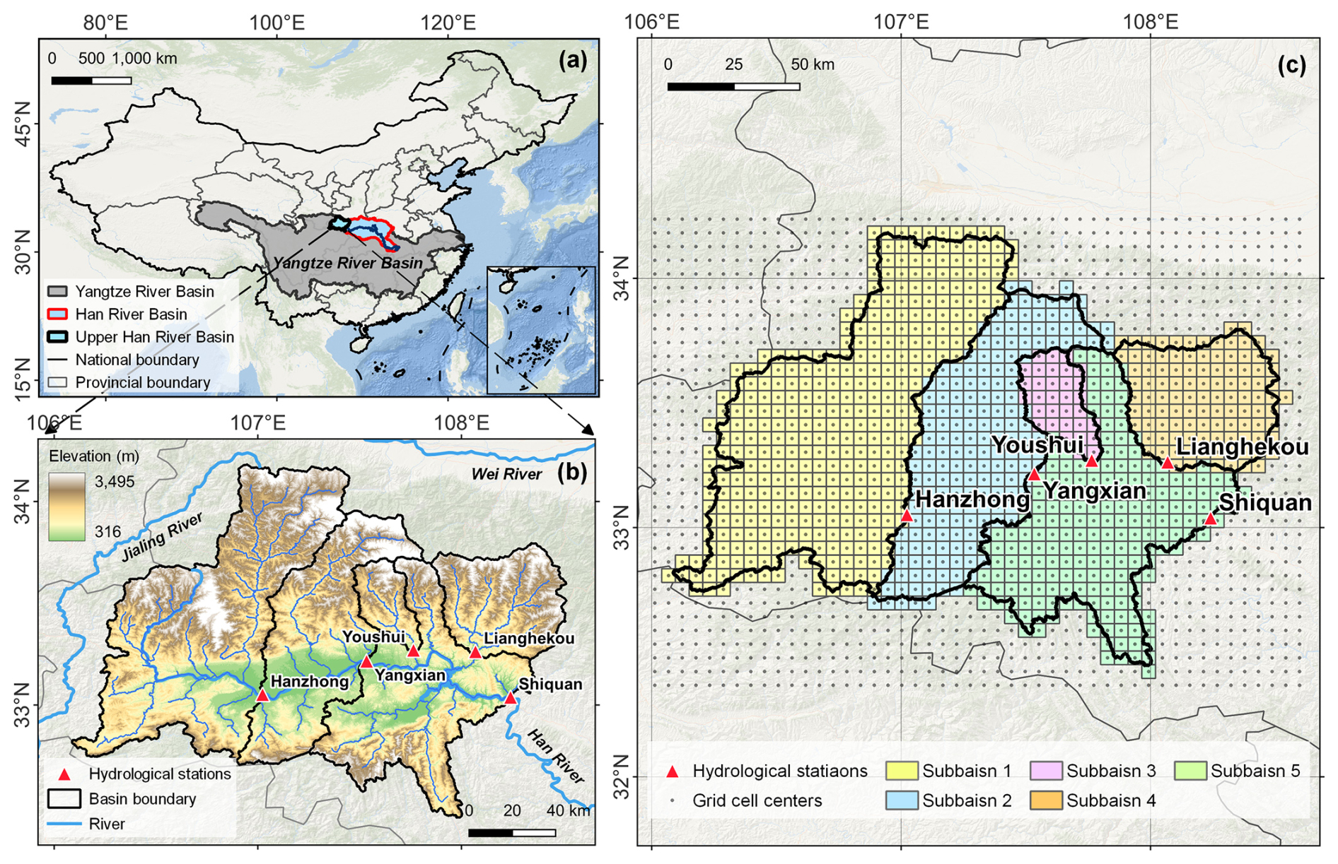
Figure 1 (a) Location of the Upper Han River Basin in China. (b) Elevation, hydrological stations, basin boundary, and river network. (c) Model domain discretized at 6 km × 6 km and the delineated five sub-basins. The background map is derived from the ESRI Ocean Basemap (Esri | Powered by Esri).

2.2 Dataset

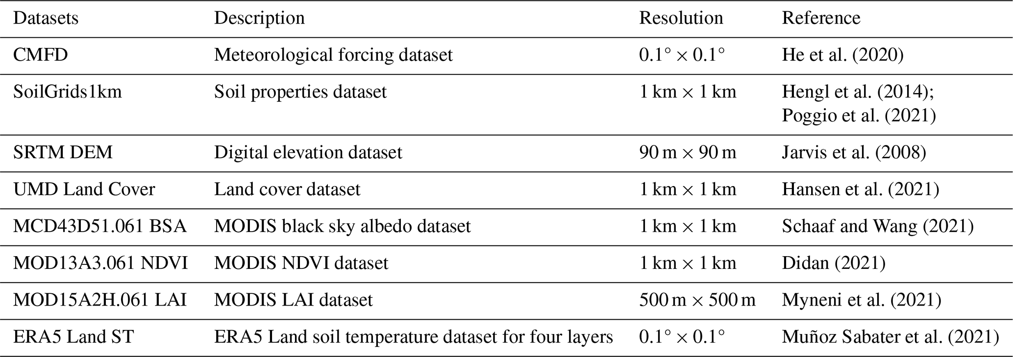
The modelling exercises of this study require a wide variety of data products, which fall into three categories: meteorological forcings, land surface characteristics, and in-situ streamflow observations. The meteorological forcings were sourced from the China Meteorological Forcing Dataset (CMFD), selected for its 3-hourly temporal resolution, which satisfies the VIC-5 image driver (hereinafter VIC-5) time-stepping scheme requirement of at least four steps per day. This dataset offers seven key meteorological variables across China at a 0.1° × 0.1° spatial resolution (1979–2018), has been widely adopted in various hydrological modelling applications (He, 2020; Sun et al., 2023).

In addition, several datasets were collected to describe the land surface characteristics (i.e., soil, topography, land cover type, and vegetation). Specifically, the soil texture (i.e., the proportions of sand, loam, and clay) and the bulk density of six soil layers at depths between 0 and 200 cm were obtained from the SoilGrids1km dataset (Poggio et al., 2021). Topography was characterized using the Shuttle Radar Topography Mission (SRTM) Digital Elevation Model (DEM) V4.1 (90 m resolution) (Jarvis et al., 2008) and land cover (14 classes) was derived from the University of Maryland's 1 km global dataset (UMD Land Cover; Hansen et al., 2021). Furthermore, monthly vegetation information – including the leaf area index (LAI), albedo, and partial vegetation cover fraction (fcanopy) – was calculated from multi-year data of several Moderate Resolution Imaging Spectroradiometer (MODIS) products (MCD43D51.061, MOD13A3.061, and MOD15A2H.061). Following established methodologies, fcanopy can be derived from the Normalized Difference Vegetation Index (NDVI) using the formula provided by Bohn and Vivoni (2019):

$$\begin{array}{}\text{(1)}& f_{\mathrm{canopy}}={\displaystyle \frac{\mathrm{NDVI}-{\mathrm{NDVI}}_{\min }}{({\mathrm{NDVI}}_{\max }-{\mathrm{NDVI}}_{\min }{)}^{\mathrm{2}}}}\end{array}$$

Then, the four-layer soil temperature from the ERA5 Land product is extracted and averaged to serve as the bottom boundary condition for the soil heat flux in the VIC model (Muñoz Sabater et al., 2021). Collectively, the land surface characteristics are integrated into a standalone parameter file for VIC-5 model execution. This parameterization entails the conversion of land surface variables into model-specific parameters, as detailed in the following section.

Finally, for model calibration and evaluation, we retrieved the observed daily streamflow records from the five hydrological stations (Fig. 1b), as published in the China Hydrological Yearbooks, and stored them in units of m³ s⁻¹. The datasets utilized in this study have varying temporal coverages; a common overlap period from 2003 to 2018 was therefore defined to ensure consistency in the modeling exercises, spanning the time during which all required model input data and streamflow records were available. Table 1 lists all the datasets used for deploying the VIC-5 model in this study.

Table 1 An overview of the datasets used for deploying the VIC-5 model.

3 Methodology

3.1 Hydrological modelling

The VIC model used for the hydrological simulation in this study was originally developed by Liang et al. (1994) as a land surface scheme within general circulation models (GCMs). As a physically based, spatially distributed hydrological model, it represents one of the most archetypal implementations of the FH69 blueprint (Freeze and Harlan, 1969), capable of simulating water and energy balances while accounting for the physical exchanges among the atmosphere, vegetation, and soil. The model is extensively used worldwide in studies of floods (Brunner et al., 2021), droughts (Lin et al., 2022), and broader water resource management (Nanditha and Mishra, 2022). For brevity, a concise overview of the VIC model is presented here, highlighting the components most pertinent to the spatially distributed parameters considered in this study, with full details available elsewhere (Melsen et al., 2016; Hamman et al., 2018; Gou et al., 2020).

The VIC model employs a structured rectangular grid for spatial discretization, with each grid cell treated as an independent runoff generation unit without lateral interactions and assigned a distinct set of parameters to reflect land surface characteristics (i.e., land cover and soil). To represent sub-grid heterogeneity, the fractional coverage of each land cover type within a cell is modelled as a separate tile and the grid-scale response is derived by aggregating the contributions of all tiles using an area-weighted average. This stochastic, non-distributed modelling approach is sometimes referred to in the literature as the variability approach (Wen et al., 2012). Through the designed structure, the parameters in the VIC model possess a naturally capacity to represent spatial variability, allowing them to be physically linked to pre-compiled information such as topography, vegetation, and soil properties. As an illustration, the saturated hydrologic conductivity can be estimated from soil texture, following the empirical formulations proposed by Cosby et al. (1984), as given below:

$$\begin{array}{}\text{(2)}& \log K_{\mathrm{s}}=\mathrm{0.0126}x-\mathrm{0.0064}y-\mathrm{0.6}\end{array}$$

where x denotes the sand content and y denotes the clay content. Overall, such transfer functions provide the conceptual foundation for regionalization approaches such as MPR.

In the VIC model, total runoff (Q_t) is partitioned into surface runoff (R) and baseflow (Q_b). Under the standard three-layer vertical soil structure (VIC-3L), surface runoff is generated from the thin top layer and the upper layer according to the variable infiltration capacity curve, as shown below (Liang et al., 1994):

$$\begin{array}{}\text{(3)}& R=\left\{\begin{array}{l}\mathrm{PE}-\left(W_{\mathrm{m}}-W_{\mathrm{0}}\right),\mathrm{PE}+i_{\mathrm{0}}\ge i_{\mathrm{m}}\\ \mathrm{PE}-\left(W_{\mathrm{m}}-W_{\mathrm{0}}\right)+W_{\mathrm{m}}{\left(\mathrm{1}-\frac{\mathrm{PE}+i_{\mathrm{0}}}{i_{\mathrm{m}}}\right)}^{\mathrm{1}+b},\\ \mathrm{PE}+i_{\mathrm{0}}<i_{\mathrm{m}}\end{array}\right.\end{array}$$

where PE denotes the effective precipitation; W_m represents the mean infiltration capacity of the grid cell; i_m is the maximum infiltration capacity at a point within the grid cell; W₀ is the initial soil moisture and i₀ is the corresponding initial infiltration capacity; and b is the shape parameter of the variable infiltration capacity curve. All of these quantities refer to the upper two soil layers. The VIC model does not explicitly represent soil drainage processes, such as interflow, or groundwater storage above the water table. Instead, these components are treated in a conceptual lumped manner and represented as baseflow from the bottom soil layer by a single term, Q_b, which is parameterized using the Arno baseflow scheme, as follows (Liang et al., 1994):

$$\begin{array}{}\text{(4)}& Q_{\mathrm{b}}=\left\{\begin{array}{l}\frac{D_{\mathrm{s}}{D}_{\mathrm{m}}}{W_{\mathrm{s}}{\mathit{\theta }}_{\mathrm{b}}^{\mathrm{s}}}\cdot {\mathit{\theta }}_{\mathrm{b}},\mathrm{0}\le {\mathit{\theta }}_{\mathrm{b}}<W_{\mathrm{s}}{\mathit{\theta }}_{\mathrm{b}}^{\mathrm{s}}\\ \frac{D_{\mathrm{s}}{D}_{\mathrm{m}}}{W_{\mathrm{s}}{\mathit{\theta }}_{\mathrm{b}}^{\mathrm{s}}}\cdot {\mathit{\theta }}_{\mathrm{b}}+(D_{\mathrm{m}}-\frac{D_{\mathrm{s}}{D}_{\mathrm{m}}}{W_{\mathrm{s}}})(\frac{{\mathit{\theta }}_{\mathrm{b}}-W_{\mathrm{s}}{\mathit{\theta }}_{\mathrm{b}}^{\mathrm{s}}}{{\mathit{\theta }}_{\mathrm{b}}^{\mathrm{s}}-W_{\mathrm{s}}{\mathit{\theta }}_{\mathrm{b}}^{\mathrm{s}}}{)}^c,\\ {\mathit{\theta }}_{\mathrm{b}}\ge W_{\mathrm{s}}{\mathit{\theta }}_{\mathrm{b}}^{\mathrm{s}}\end{array}\right.\end{array}$$

where ${\mathit{\theta }}_{\mathrm{b}}^{\mathrm{s}}$ is the maximum soil moisture of the bottom layer; D_m is the maximum baseflow; D_s is the fraction of D_m at which nonlinear baseflow begins; W_s is the fraction of ${\mathit{\theta }}_{\mathrm{b}}^{\mathrm{s}}$ at which nonlinear baseflow begins; and c is the exponent of the nonlinear part of the Arno baseflow curve, which is usually set to 2. All of these quantities refer to the bottom soil layer. The Arno baseflow equation can be equivalently reformulated as a coupled linear reservoir and a nonlinear reservoir, and can thus be expressed in the following form, thereby alleviating parameter interactions (Nijssen et al., 2001):

$$\begin{array}{}\text{(5)}& Q_{\mathrm{b}}=\left\{\begin{array}{ll}{D}_{\mathrm{1}}{\mathit{\theta }}_{\mathrm{b}},& \mathrm{0}\le {\mathit{\theta }}_{\mathrm{b}}<D_{\mathrm{3}}\\ D_{\mathrm{1}}{\mathit{\theta }}_{\mathrm{b}}+D_{\mathrm{2}}({\mathit{\theta }}_{\mathrm{b}}-D_{\mathrm{3}}{)}^{D_{\mathrm{4}}},& {\mathit{\theta }}_{\mathrm{b}}\ge D_{\mathrm{3}}\end{array}\right.\end{array}$$

where D₁ is the linear reservoir coefficient; D₂ is the nonlinear reservoir coefficient; D₃ denotes soil moisture at which baseflow transition occurs from linear to nonlinear; and D₄ has the same conceptual meaning as c. This formulation is also known as the Nijssen form of the Arno model, has been incorporated into the official VIC model and can be specified through the global parameter file.

The complete rainfall-runoff process comprises both runoff generation and routing stages. The RVIC model was proposed as a post-processor of the VIC model, designed to trace river channel flow by a pre-defined Unit Hydrograph (UH) and generate hydrographs at specified outlet points (Lohmann et al., 1996). The principle of RVIC can be briefly described as the solution of the linear Saint-Venant equations within a linear time-invariant system. Its primary parameters, flow velocity and diffusion coefficient, are generally treated either as spatially uniform free parameters to be calibrated or as fixed constants in the absence of observations. To date, RVIC remains the official extension of the VIC-5 and its earlier version, and has seen broad application (Shrestha et al., 2025).

Here, the VIC-5 image driver version and RVIC are consistently deployed at 6 km × 6 km spatial resolution (Fig. 1c) with a 3-hourly timestep, and the simulated output are aggregated to the daily timestep for calibration and evaluation. For the parameter estimation and calibration procedures, detailed descriptions are provided in the following sections.

3.2 Multiscale parameter regionalization with VIC-specific refinement

Samaniego et al. (2010) introduced a hierarchy of spatial scales to distinguish information across different resolution, which provides a basis for MPR implementation. Following this concept, we define the observational resolution describing land-surface characteristics as the level-0 scale (i.e., 1 km), while modelling resolution is represented by the level-1 scale (i.e., 6 km), reflecting the principal process scale resolved by the model. As introduced before, the MPR technique is model-independent, and its application to the VIC model requires specific refinement. Specifically, for each VIC parameter, we identify applicable prior transfer functions from literature and generalize them into a scale-independent form by incorporating the g-parameters. Using Eq. (2) as an example, we generalize it into the following form:

$$\begin{array}{}\text{(6)}& K_{\mathrm{s}}={\mathrm{10}}^{g_{\mathrm{1}}x+g_{\mathrm{2}}y+g_{\mathrm{3}}}\end{array}$$

where g_i constitutes a set of g-parameters to be calibrated. For clarity and tractability, refinement is applied exclusively to several sensitive parameters (Gou et al., 2020), while the coefficients in the transfer functions of all other parameters are retained at their prior values (Mizukami et al., 2017), thus mitigating the issues arising from the curse of dimensionality. Table 2 summarizes the VIC-specific refinement of MPR. It is worth noting that VIC supports two equivalent baseflow parameterizations. Following Mizukami et al. (2017), we adopt the Nijssen formulation (i.e., D₁, D₂ and D₃) to avoid the parameter interactions present in the original Arno formulation (Eq. 5). Namely, calibration of D₁, D₂ and D₃ is equivalent to calibrating D_s, D_m and W_s, which have been identified as sensitive parameters in previous studies (Wen et al., 2012; Gou et al., 2021).

Table 2 VIC-specific refinement of MPR, detailing the transfer functions and the sources of the corresponding formulations.

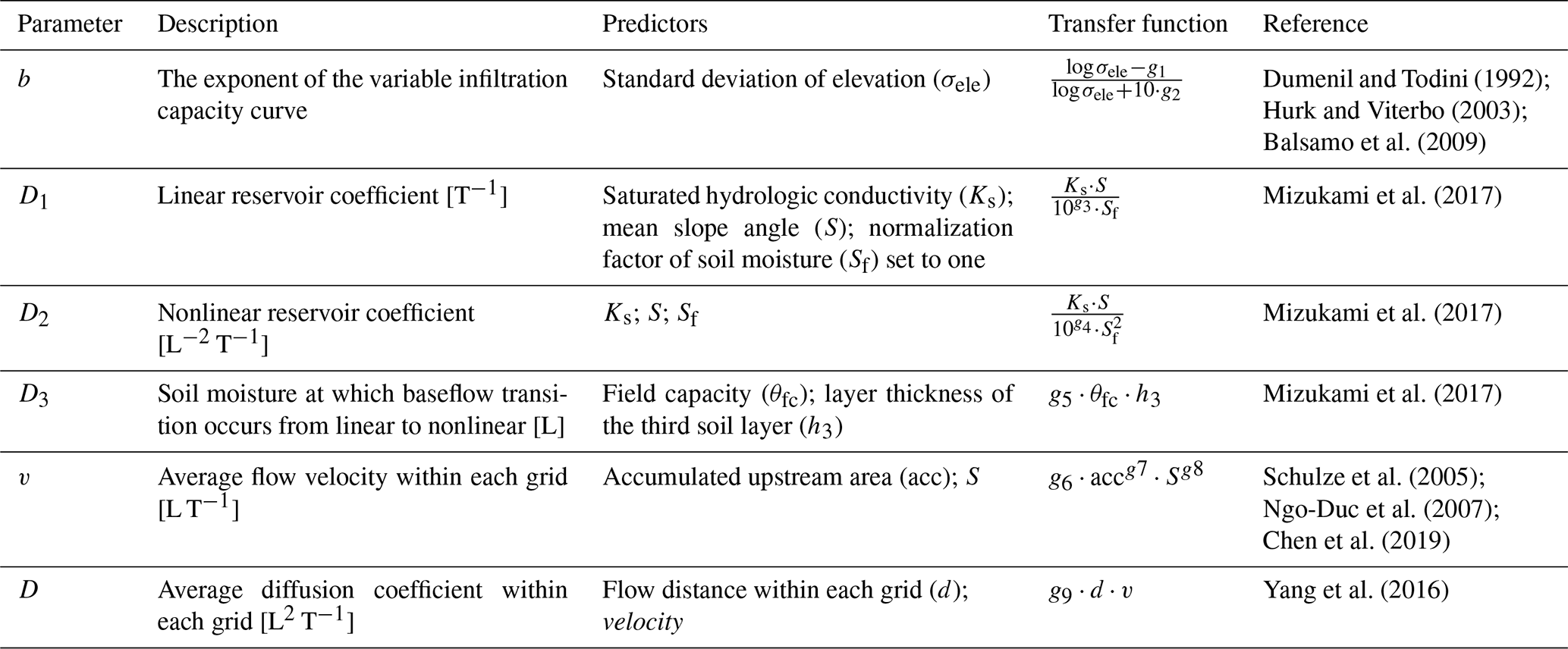
^* Note: Units are K_s (mm s⁻¹), S (%), θ_fc (m³ m⁻³), h₃ (m), acc (km²), and d (m).

Besides the spatially explicit parameterization of soil hydraulic-related parameters (b, D₁, D₂, and D₃), two additional refinements were made to parameters that exert strong control on runoff generation and concentration. First, it is widely recognized among the VIC users that the vertically discretized soil depth is a key determinant of runoff generation. In the classic VIC-3L (i.e., VIC three-layer) configuration, the upper two soil layers respond rapidly to precipitation, generating surface flow according to the Xinanjiang formulation, whereas the bottom layer governs baseflow, resulting in a slower runoff response (Eqs. 3 and 5). Different soil layer thicknesses produce significantly different runoff responses; consequently, these thicknesses (h₁, h₂, and h₃) are typically treated as free parameters during calibration to fine-tune the VIC behavior (Gou et al., 2020). In addition, the original soil dataset (i.e., SoilGrids1km) provides six soil layers, each characterized by distinct properties (e.g., soil texture), whereas VIC-3L adopts a three-layer soil structure. In order to feed original soil data into the transfer function, it is necessary to reconcile its soil-layer structure with the VIC vertical structure. As shown in Fig. 2, a two-step mechanism is applied here, involving aggregation and scaling. In the first step, the original soil data are aggregated into a standard three-layer structure defined by the layering numbers z₁ and z₂, with the corresponding layer thicknesses summed and the soil properties averaged within each standard layer. In the second step, the original thickness (h₀) is scaled by g₁₀ to allow flexible adjustment of the final computational layer thickness. This mechanism is applicable to most soil-column-based hydrological models and has been validated in Mizukami et al. (2017). However, previous implementations used domain-wide uniform values of z₁, z₂, and g₁₀, a simplification that diminished the representation of spatial heterogeneity in soil layer depths and reflected the limited availability of spatially grounded information on vertical soil structure. In this study, we compare simulations using uniform depths with those employing subbasin-unique depths (i.e., subbasin-specific values of z₁, z₂, and g₁₀), analogous to a semi-distributed scheme, to examine how spatially explicit parameterization alter model behavior.

Second, the refinement is applied to the RVIC parameters, velocity (v) and diffusion (D), respectively. In previous studies, these two parameters were generally considered constant or spatially uniform free parameters to be calibrated (Shrestha et al., 2025; Yousefi Sohi et al., 2024). The official VIC documentation also recommends a diffusivity of 800 m² s⁻¹ and a velocity of 1.5 m s⁻¹ as acceptable values (https://vic.readthedocs.io/en/vic.4.2.d/Documentation/Calibration, last access: 25 April 2026). Nonetheless, we use the MPR technique here to enhance the spatial representation of these two parameters by linking them to topography (Fig. S2). This enhancement is then assessed for its impact on model behavior, which is particularly relevant for applications with limited prior information on channel routing, such as Manning's coefficients or channel morphology. Additionally, RVIC relies on UH as the impulse response function to convert runoff into streamflow, requiring them to be predefined. While various types of UH exist, such as the dimensionless SCS UH and the Nash UH (Roy and Thomas, 2016), the general UH (GUH) has drawn our attention due to its analytical formulation (Guo, 2022), with its expression presented as follows:

$$\begin{array}{}\text{(7)}& {\displaystyle }u\left(t\right)={\displaystyle \frac{\mathrm{d}g}{\mathrm{d}t}}={\displaystyle \frac{\mathit{\mu }}{t_{\mathrm{p}}}}x(\mathrm{1}+mx{)}^{-(\mathrm{1}+\mathrm{1}/m)}\text{(8)}& {\displaystyle }g\left(t\right)=\mathrm{1}-(\mathrm{1}+mx{)}^{-\mathrm{1}/m}\text{(9)}& {\displaystyle }x\left(t\right)=\exp \left[\left(\mathit{\mu }\left({\displaystyle \frac{t}{t_{\mathrm{p}}}}-\mathrm{1}\right)\right)\right]\end{array}$$

where t_p is the peak flow time; m is a dimensionless recessing coefficient that is determined by the downstream water surface condition; and μ is the rising coefficient related to the basin characteristics. By calibrating the three parameters, the shape of the GUH can be freely adjusted, thereby providing flexibility in model representation when prior knowledge is limited. The GUH also demonstrate several advantages, including a solid theoretical and mathematical foundation (i.e., the solution of Chow's linear hydrologic systems equations), the ability to reproduce typical flood responses with high accuracy, and, under certain conditions, the capacity to closely approximate traditional unit hydrographs. Based on this, we select it as the engine for RVIC, which acts as grid UH over the domain.

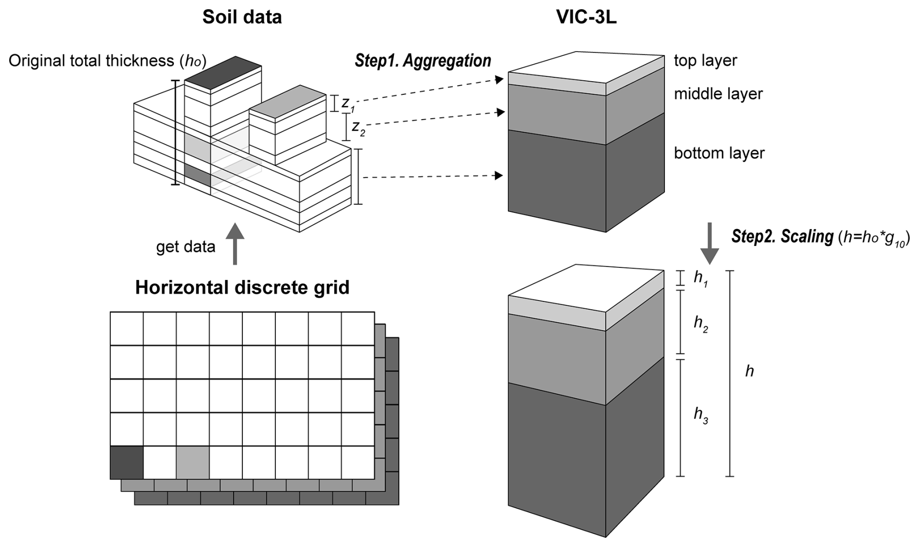
Figure 2 Schematic of the two-step mechanism for reconciling soil data with VIC three-layer (VIC-3L) vertical structure. In the aggregation step, the original soil layers are merged into three VIC soil layers based on the layering numbers z₁ and z₂. The scaling step then applies a scaling factor (g₁₀) to the original total thickness (h_o) to obtain the model-prepared layer thicknesses h₁, h₂, and h₃.

3.3 Experiment framework for spatially explicit parameterization and multi-gauge calibration

For this study, we design an Experiment Framework to evaluate the effect of Spatially explicit Parameterization and Multi-gauge calibration, termed EF-SPM. The eight calibration cases, differing in their configurations of parameterization and calibration objectives, are summarized in Table 3. By grouping and comparing these cases, we can derive seven experiments with clearly defined objectives (Table 4), and can organize them into the following four main experimental setups. The EF-SPM experimental framework is illustrated in Fig. 3. For clarity and ease of understanding, the terms “distributed” and “spatially explicit” are used interchangeably below, unless otherwise noted.

• Experiment 1. The added value of spatially explicit parameterization.

  This experiment compares the calibration process and simulations between the fully spatially explicit (distributed) and spatial uniform parameter configurations to identify the effects of spatially explicit parameterization on model behaviour. Here, the calibration objective was treated as the controlled condition. Cases 7 and 8 were compared under the single-gauge calibration, while Cases 1 and 5 were compared under the multi-gauge calibration.

• Experiment 2. The role of multi-gauge calibration.

  With the parameterization scheme (Distributed vs. Uniform) as a controlled variable, this experiment assesses the advantage of multi-gauge calibration for parameter identification and model improvement, via comparisons between Case 5 and Case 8 (distributed) and between Case 1 and Case 7 (uniform). Note that Exp. 1 and 2 are orthogonally designed to decouple the independent and interactive effects of spatial complexity and calibration strategy, which thus ensures a distinct and non-redundant comparison within a rigorous 2 × 2 framework and thereby facilitates our exploration of the potential cross-benefits between these two methodological dimensions.

• Experiment 3. Benefit of the additional MPR refinements.

  As outlined in the previous section, additional refinements were applied to the soil layer depths and RVIC parameters to enhance their spatial representativeness. This experiment evaluates the impact of this refinement strategy on model behaviour. Under controlled conditions, the contrast between Case 4 and Case 5 isolates the effect of spatially explicit soil layer depths (specifically, values assigned per the sub-basin delineation in Fig. 1c), while the progression from Case 3 to Case 2 to Case 4 quantifies the impact of progressively increased RVIC complexity.

• Experiment 4. Performance Evolution from Baseline to Full-Complexity setup.

  Finally, the joint effects of these configurations are evaluated by comparing the simplest configuration (Case 6) against the most complex one (Case 5).

  As detailed in Table 5, the parameter count for the fully distributed parameterization is over double that of the fully uniform one. We anticipate that refining spatial representation of parameters will enhance model performance, yet also compromise parameter identifiability. Whether this can be paired with better calibration to enhance model realism is the key question we seek to answer. The parameters to be calibrated in the EF-SPM experimental framework, along with their descriptions and feasible ranges, are summarized in Table 6.

Table 3 Overview of the calibration cases with different configurations.

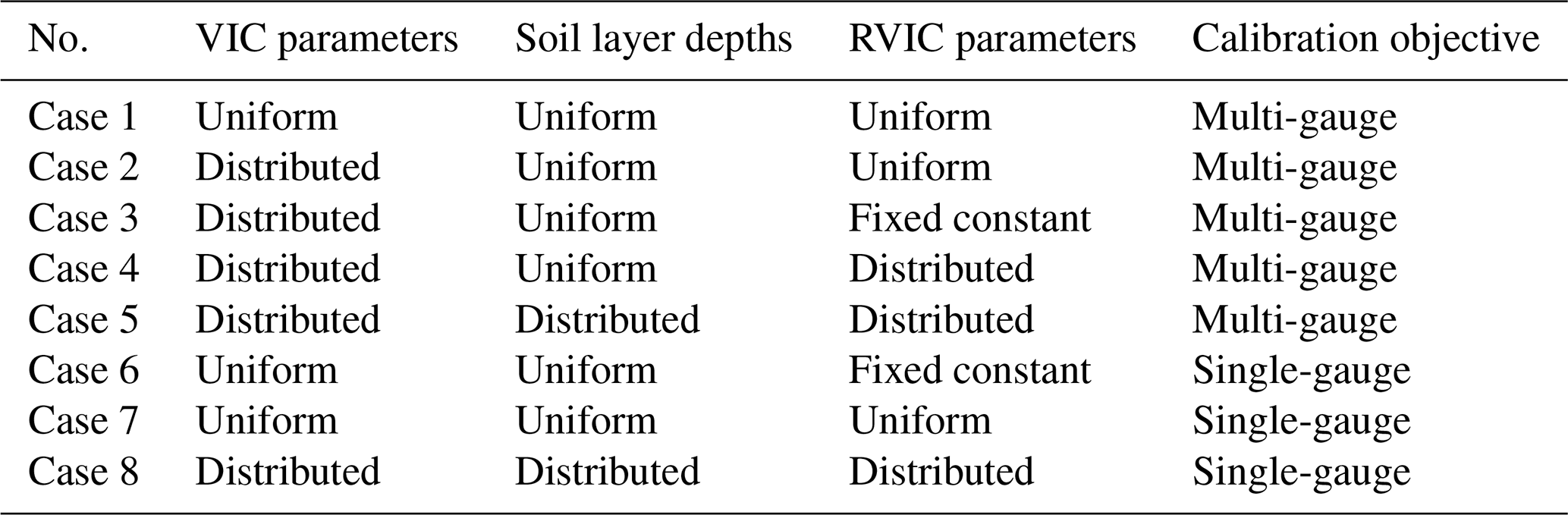
Table 4 Summary of experiments within the EF-SPM framework, showing the cases considered, the configurations compared, and their purposes.

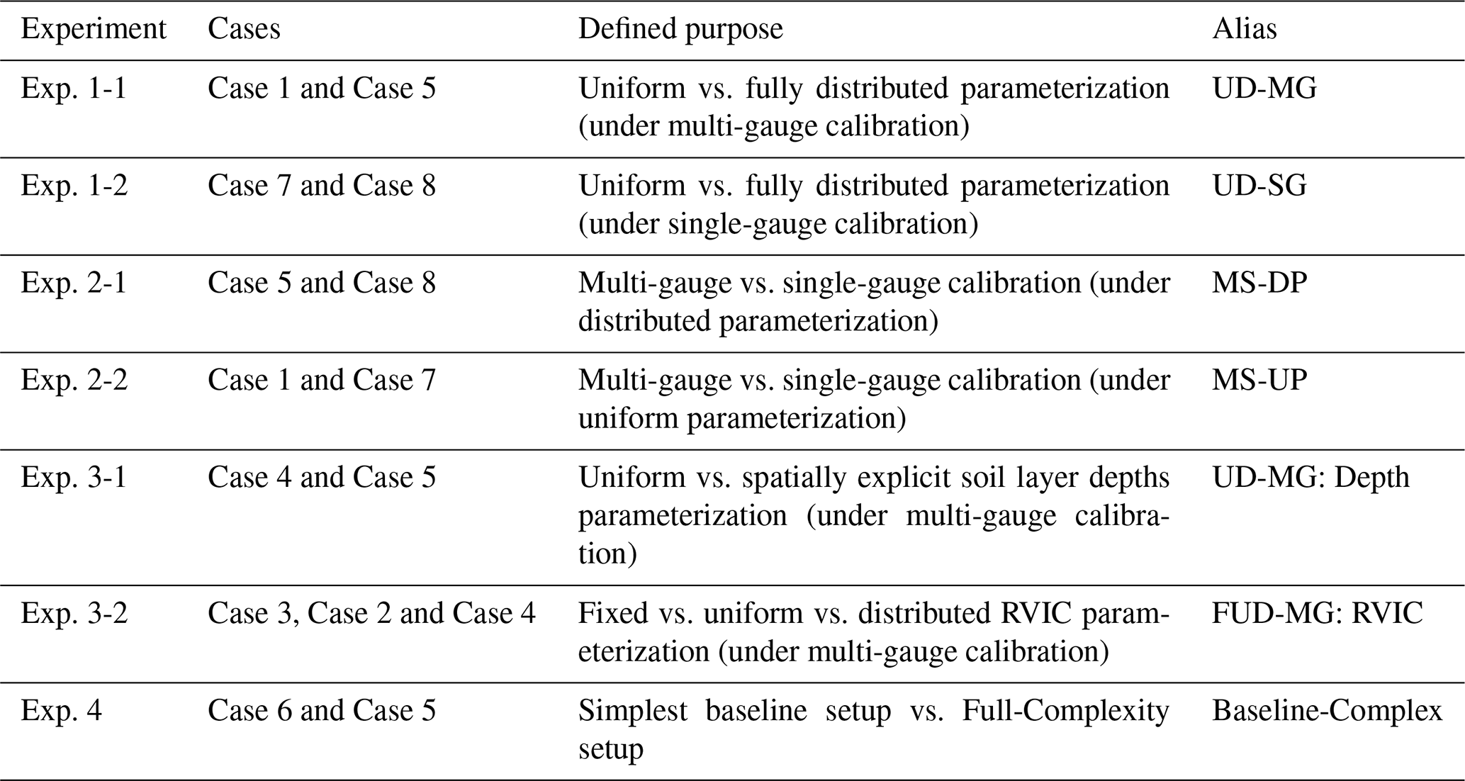
^* Alias abbreviation: UD = uniform vs. distributed parameterization; MS = multi-gauge vs. single-gauge calibration; FUD = fixed vs. uniform vs. distributed parameterization; MG = multi-gauge calibration; SG = single-gauge calibration; DP = distributed parameterization; Depth = soil layer depths; RVIC = RVIC-specific parameterization; Baseline-Complex = Simplest baseline setup vs. Full-Complexity setup.

Table 5 Total number of parameters for the uniform and distributed parameterization.

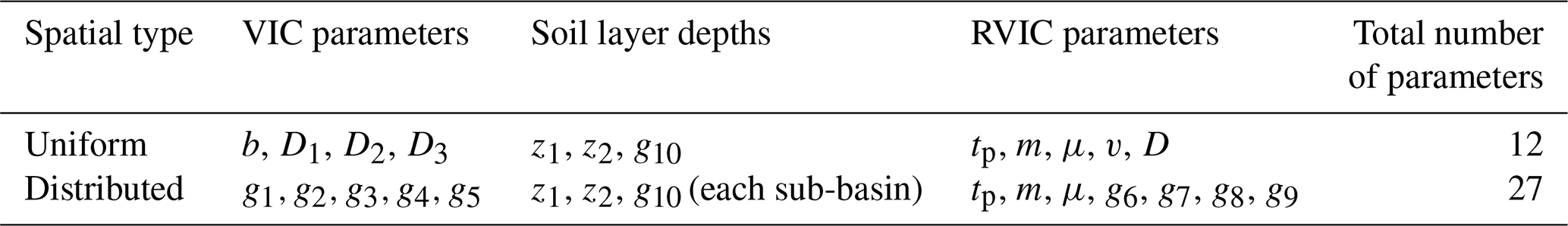
^* Note: A total of five sub-basins are employed in this study.

Table 6 Description and feasible ranges of the free parameters subject to calibration.

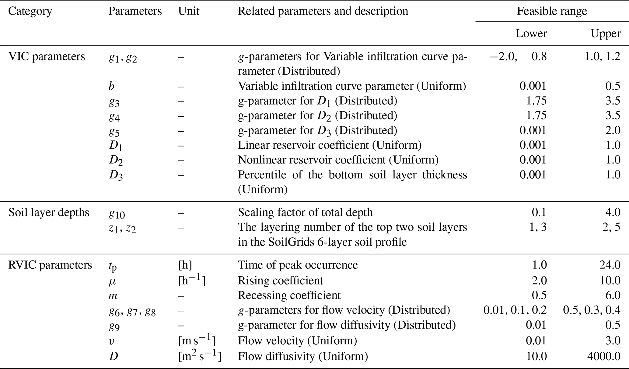
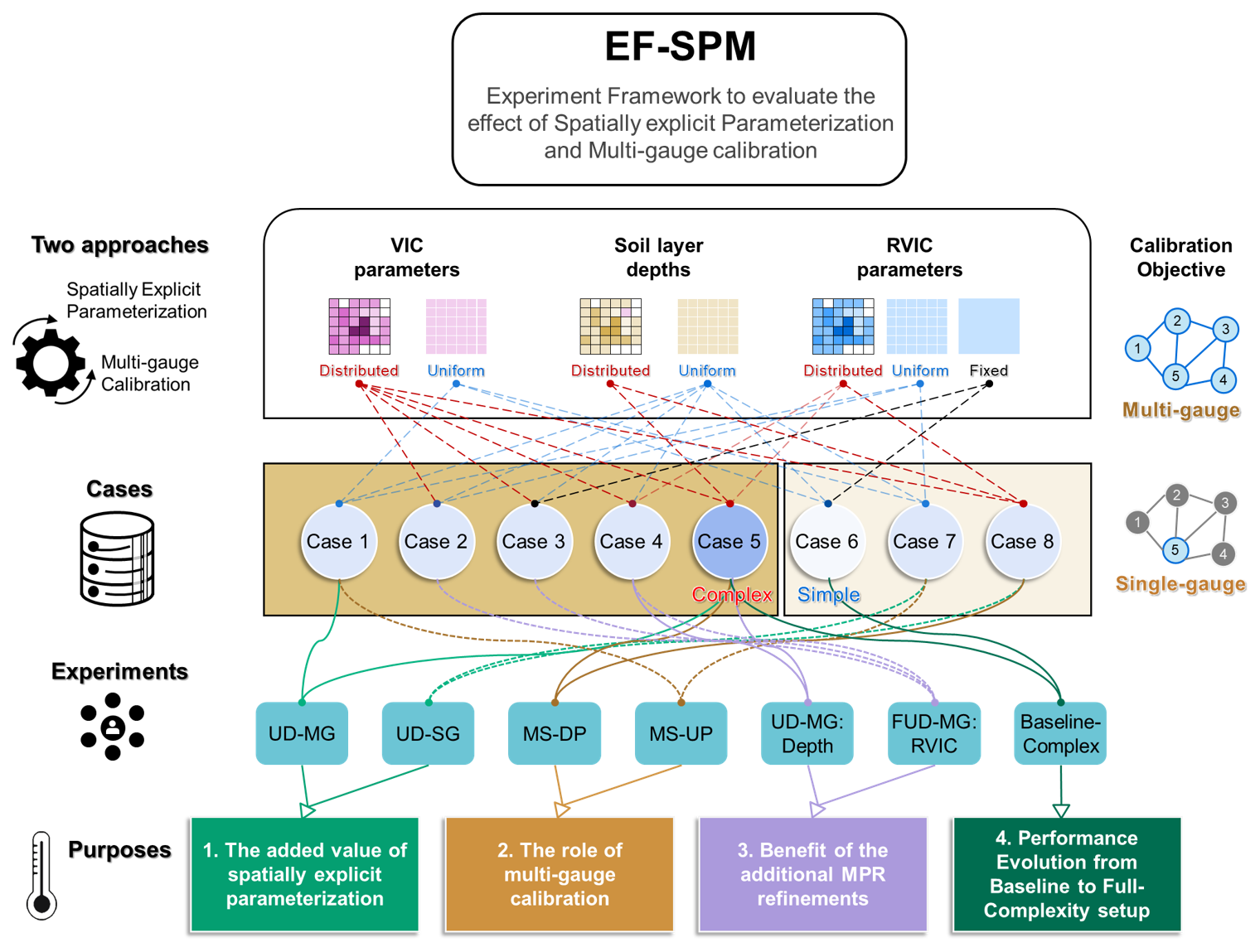
Figure 3 Schematic illustration of the Experiment Framework to evaluate the effect of Spatially explicit Parameterization and Multi-gauge calibration (EF-SPM).

3.4 Optimization algorithms and evaluation metrics

Different algorithms were employed for single-objective and multi-objective calibration. For the former, we used the Covariance Matrix Adaptation Evolution Strategy (CMA-ES; Hansen and Ostermeier, 2001), a global, single-objective optimizer based on a generate-and-update paradigm that has demonstrated robust performance in hydrological model calibration (Knoben et al., 2020; Aerts et al., 2024). For multi-objective calibration, we likewise adopted an evolution strategy, the Non-dominated Sorting Genetic Algorithm II (NSGA-II), to ensure a fair comparison by minimizing algorithmic bias. We implemented all optimization algorithms with the DEAP Python package (De Rainville et al., 2012; Fortin et al., 2012). In addition, both optimizers were configured with an identical population size of 20 and shared the same objective function: the modified Kling-Gupta efficiency (KGE) of the streamflow, with the only difference being the number of gauges considered in each case, as given below (Aerts et al., 2022):

$$\begin{array}{}\text{(10)}& \mathrm{KGE}=\mathrm{1}-\sqrt{(r-\mathrm{1}{)}^{\mathrm{2}}+{\left({\displaystyle \frac{{\mathit{\mu }}_{\mathrm{sim}}}{{\mathit{\mu }}_{\mathrm{obs}}}}-\mathrm{1}\right)}^{\mathrm{2}}+{\left({\displaystyle \frac{{\mathit{\sigma }}_{\mathrm{sim}}/{\mathit{\mu }}_{\mathrm{sim}}}{{\mathit{\sigma }}_{\mathrm{obs}}/{\mathit{\mu }}_{\mathrm{obs}}}}-\mathrm{1}\right)}^{\mathrm{2}}}\end{array}$$

where r is the linear correlation coefficient between observed (obs) and simulated flow (sim), while σand μ denote their respective stand deviations and means. The three terms in Eq. (10) represent, respectively, the correlation between observations and simulations (r), the bias in the mean (β), and the bias in the variability (γ). For both the KGE and its individual components, a value closer to 1 denotes better model performance, with 1 representing perfect agreement. Under the two optimization algorithms, CMA-ES optimizes the KGE at the basin outlet (Shiquan) as the single-objective function (KGE_Q5), whereas NSGA-II performs multi-objective optimization in the multi-dimensional Pareto space, considering the KGE of streamflow at the five subbasin gauges as separate objectives (KGE_Q1, KGE_Q2, KGE_Q3, KGE_Q4, KGE_Q5).

To further support a comprehensive evaluation, we additionally considered several signature metrics, as highlighted in the diagnostic evaluation framework (Gupta et al., 2008). Unlike aggregated performance metrics, hydrologic signatures offer a quantitative measure of specific hydrograph properties or behavior (e.g., total volume, flow peaks, and recession limbs). This allows for a more refined characterization of the temporal dynamics inherent in hydrography and helps pinpoint specific discrepancies in simulated flow patterns. Following Yilmaz et al. (2008) and Casper et al. (2012), a suite of flow duration curve (FDC)-based bias metrics was adopted. Specifically, %PBias was used to characterize overall water volume differences; %BiasFHV quantifies discrepancies in the high-flow segment; %BiasFLV represents differences in the low-flow segment; %BiasFMS describes deviations in the slope of the middle segment; and %BiasFMM measures the percentage differences in mid-range flow levels. The corresponding formulations are given below:

$$\begin{array}{}\text{(11)}& {\displaystyle }\mathrm{\%}\mathrm{PBias}={\displaystyle \frac{{\sum }_{i=\mathrm{1}}^N(Q_{\mathrm{sim}}^i-Q_{\mathrm{obs}}^i)}{{\sum }_{i=\mathrm{1}}^n{Q}_{\mathrm{obs}}^i}}\times \mathrm{100}\mathit{\%}\text{(12)}& {\displaystyle }\mathrm{\%}\mathrm{BiasFHV}={\displaystyle \frac{{\sum }_{h=\mathrm{1}}^H(Q_{\mathrm{sim}}^h-Q_{\mathrm{obs}}^h)}{{\sum }_{h=\mathrm{1}}^H{Q}_{\mathrm{obs}}^h}}\times \mathrm{100}\mathit{\%}\text{(13)}& {\displaystyle }\mathrm{\%}\mathrm{BiasFLV}={\displaystyle \frac{\begin{array}{c}{\sum }_{l=\mathrm{1}}^L\left[\log \left(Q_{\mathrm{sim}}^l\right)-\log \left(Q_{\mathrm{sim}}^{\min }\right)\right]\\ -{\sum }_{l=\mathrm{1}}^L\left[\log \left(Q_{\mathrm{obs}}^l\right)-\log \left(Q_{\mathrm{obs}}^{\min }\right)\right]\end{array}}{{\sum }_{l=\mathrm{1}}^L\left[\log \left(Q_{\mathrm{obs}}^l\right)-\log \left(Q_{\mathrm{obs}}^{\min }\right)\right]}}\times \mathrm{100}\mathit{\%}\text{(14)}& {\displaystyle }\mathrm{\%}\mathrm{BiasFMS}={\displaystyle \frac{\begin{array}{c}\left[\log \left(Q_{\mathrm{sim}}^{m\mathrm{1}}\right)-\log \left(Q_{\mathrm{sim}}^{m\mathrm{2}}\right)\right]\\ -\left[\log \left(Q_{\mathrm{obs}}^{m\mathrm{1}}\right)-\log \left(Q_{\mathrm{obs}}^{m\mathrm{2}}\right)\right]\end{array}}{\left[\log \left(Q_{\mathrm{obs}}^{m\mathrm{1}}\right)-\log \left(Q_{\mathrm{obs}}^{m\mathrm{2}}\right)\right]}}\times \mathrm{100}\mathit{\%}\text{(15)}& {\displaystyle }\mathrm{\%}\mathrm{BiasFMM}={\displaystyle \frac{\mathrm{Median}\left(Q_{\mathrm{sim}}\right)-\mathrm{Median}\left(Q_{\mathrm{obs}}\right)}{\mathrm{Median}\left(Q_{\mathrm{obs}}\right)}}\times \mathrm{100}\mathit{\%}\end{array}$$

where Q denotes the streamflow; i=1, 2, … , N, h=1, 2, … , H, and l=1, 2, … , L are the indices of flow value in the full record, the high-flow segment (exceedance probabilities of 0–0.02 for %BiasFHV₂ and 0–0.01 for %BiasFHV₁), and low-flow segment (defined as 0.7–1.0) of the flow duration curve, respectively. The middle-flow segment is bounded by two thresholds, m1 and m2, corresponding to exceedance probabilities of 0.2 and 0.7, respectively. Note that the original definitions were slightly modified here to ensure consistent sign conventions across all metrics, where negative values indicate an underestimation by the simulations.

The full period from 2003 to 2018 was allocated for warm-up (2003–2004), calibration (2005–2014), and validation (2015–2018) in a $\mathrm{1}:\mathrm{5}:\mathrm{2}$ ratio. To ensure computational efficiency while maintaining calibration performance, we conducted 40 calibration trials for each case (amounting to 40 trials × 20 individuals = 800 model runs in total), a number we found sufficient to ensure convergence based on our preliminary tests. All cases implemented in this study were deployed using the Easy VIC Build (EVB) open-source Python framework developed by our team (https://github.com/XudongZhengSteven/easy_vic_build, last access: 25 April 2026), which was designed to streamline the deployment process of the VIC model.

4 Results and discussion

4.1 Comparative overview of model performance

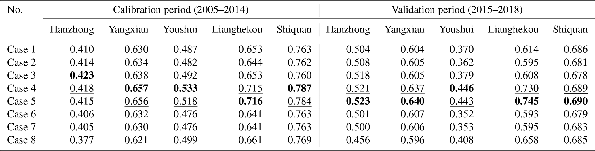
In this section, we first present an overview of the KGE-based streamflow simulation performance across all cases within the EF-SPM. To mitigate calibration uncertainty, the ensemble-mean KGE derived from the five optimal solution sets is reported, synthesizing results from multiple calibration trials (Table 7). As shown, Case 5 and 4 account for the first- and second-best performances in nearly all cases, for both calibration and validation. This behavior is in line with expectations, given that these cases involve a more explicit representation of spatial parameters and tighter calibration constraints. A comparable pattern of enhancement emerges when transitioning from simpler to more complex configurations (e.g., Case 6 to Case 8, and Cases 1–3 to Cases 4–5). Notably, the most substantial performance gain was observed when moving from the simplest (Case 6) to the most complex configuration (Case 5), as anticipated in Exp. 4 (Baseline-Complex). In addition, a spatial dimension to performance differences was also observed, where upstream headwater sub-basins (e.g., Hanzhong and Youshui) consistently underperformed relative to downstream locations.

To further examine the statistical significance of performance differences across various cases, we conducted pairwise t-tests on the KGE at the Shiquan station (basin outlet), as shown in Table S1. It is evident that, at a significance level of 0.05, Case 4 performs significantly better than all other cases, while Case 8 performs significantly worse than all other cases. Moreover, the patterns identified in the previous analysis are further confirmed by this significance test, with the more complex configurations generally outperforming the simpler ones. It is worth noting that this comparison is conducted under a single-objective context, as Cases 6–8 only consider streamflow at the basin outlet as objective functions.

The initial analyses are encouraging, demonstrating that improvements in spatial parameter explicitness and multi-gauge calibration consistently lead to better streamflow reproduction. In particular, the overall simulation performance is satisfactory at the basin outlet (Shiquan station), with calibration KGE exceeding 0.76 across all cases and validation KGE values remaining above 0.67. The results presented here establish the context for analyzing the specific effects of these configuration.

Table 7 Overview of ensemble mean performance metrics (KGE) for all calibration cases. Best values are highlighted in bold, with second-best values underlined.

4.2 Spatially explicit parameterization: impact and trade-off analysis

The refinement of spatial representation involves three parameter groups: VIC parameters, soil layer depths, and RVIC parameters. To maintain analytical clarity, this section focuses solely on evaluating their combined effect on simulation in Exp. 1 (Case 1 vs. Case 5 [UD-MG] and Case 7 vs. Case 8 [UD-SG]), leaving the analysis of their individual effects from Exp. 3 to a subsequent section. Note that, for robustness, all results herein represent the ensemble values of the top five optimal solutions, consistent with the previous section.

4.2.1 Hydrograph simulation

We first sought to determine whether enhanced spatial parameterization alters the behavior of the hydrograph – i.e., the integrated hydrological response. A comparison of the overall simulation patterns for the four cases in Exp. 1 at the Shiquan station during the validation period, presented in the observed-simulated streamflow space in Fig. 4, indicates a consistent systematic underestimation bias across all configurations. Among these, the cases representing distributed parameterization (Cases 5 and 8, shown in blue) visibly outperform those with uniform parameterization (shown in red), as demonstrated by their closer alignment with the 1:1 line. In terms of calibration strategy, the multi-gauge calibration appears to be superior. This is exemplified by Case 5, which yields a regression slope of 0.74 – the highest among all cases and closest to the ideal value of 1.

Next, we evaluated the simulation discrepancies across different hydrological conditions based on the FDCs (Ma et al., 2024), as presented in Fig. 5. A clear pattern is that, for the shared target station (Shiquan), FDCs align more closely under the same parameterization (i.e., Case 1 with Case 7, and Case 5 with Case 8), suggesting that parameterization exerts a greater influence on the simulation pattern than calibration configuration. In general, spatially explicit parameterization (Cases 5 and 8) offer improved simulation of the high-flow segment, yielding higher peak values (as shown in the box-and-scatter representation Fig. 5); however, this comes at the expense of accurately capturing extreme low flows, namely, an overestimation of baseflow. This behaviour is also evident in the scatter comparison on a logarithmic scale (Fig. S3).

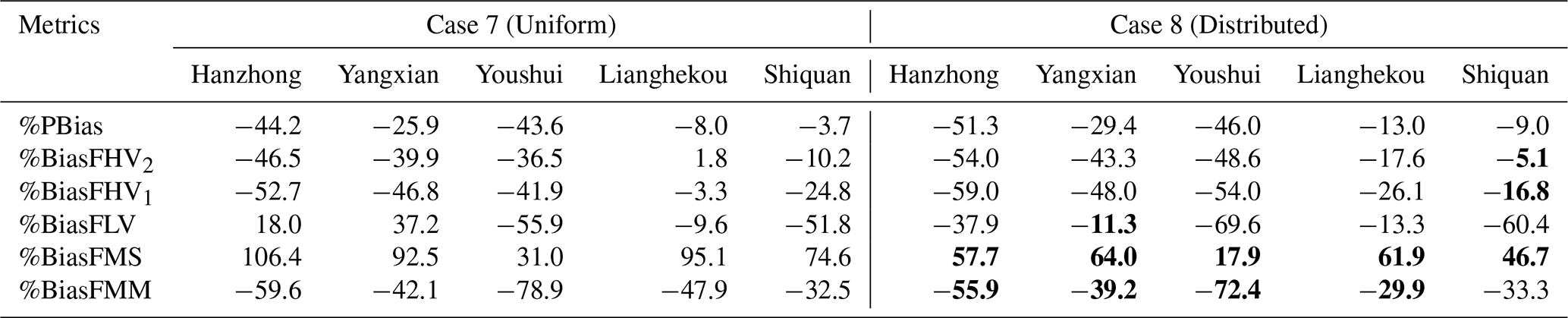
The signature metrics in Tables 8 and 9 provide quantitative support for the above behaviour at the Shiquan station: the shift from uniform to spatially explicit parameterization enhances %BiasFHV₂ by 5 % and 7 % (absolute change), and improves %BiasFHV₁ even more substantially (by 8 % and 18 %), while simultaneously worsening %BiasFLV by 0.6 % and 8.6 %, under both multi-gauge and single-gauge calibration setups. Importantly, attention is drawn to the nearly universal improvement in the mid-FDC segment from Cases 1/7 to Cases 5/8. This consistent pattern across all stations provides compelling evidence for the benefits afforded by spatially explicit parameterization. Additionally, single-gauge calibration shows a compensatory effect, where increasing model complexity improves high-flow simulation at the target gauge but degrades performance at all other sites (Table 9). This illustrates an under-constrained inverse problem, a limitation that is alleviated by multi-gauge calibration and will be explored in detail in a later section.

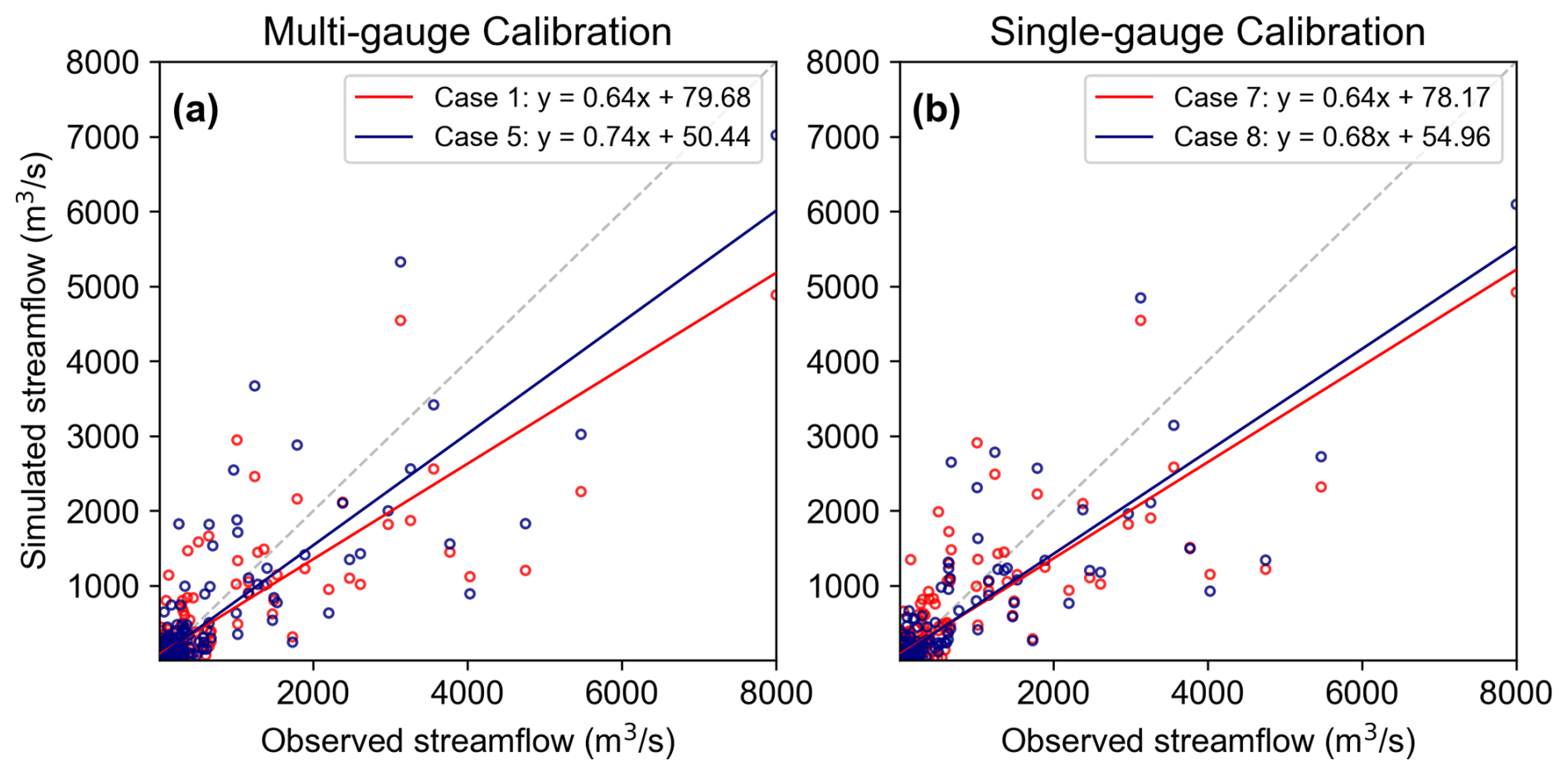
Figure 4 Scatterplots with least-squares regression lines comparing observed and simulated daily streamflow at the Shiquan station during the validation period, under different case configurations. The grey dashed line represents the 1:1 line. Flows below 1000 m³ s⁻¹ were randomly thinned for clarity.

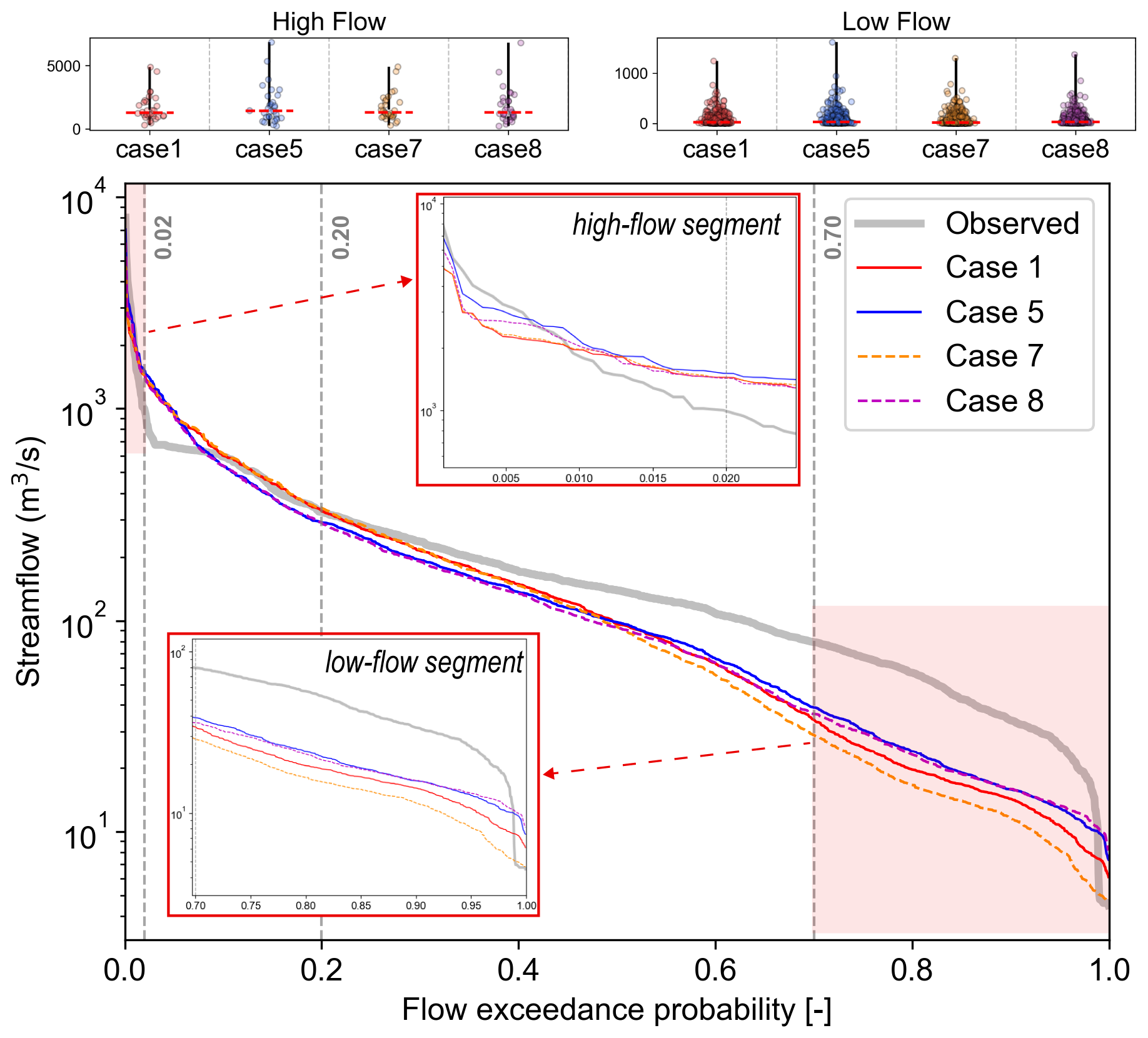
Figure 5 Comparison of observed and simulated flow duration curves for different case configurations at the Shiquan station during the validation period.

Table 8 Comparison of hydrologic signature metrics during the validation period under multi-gauge calibration: Case 1 versus Case 5. Bold values indicate where Case 5 shows improved performance relative to Case 1.

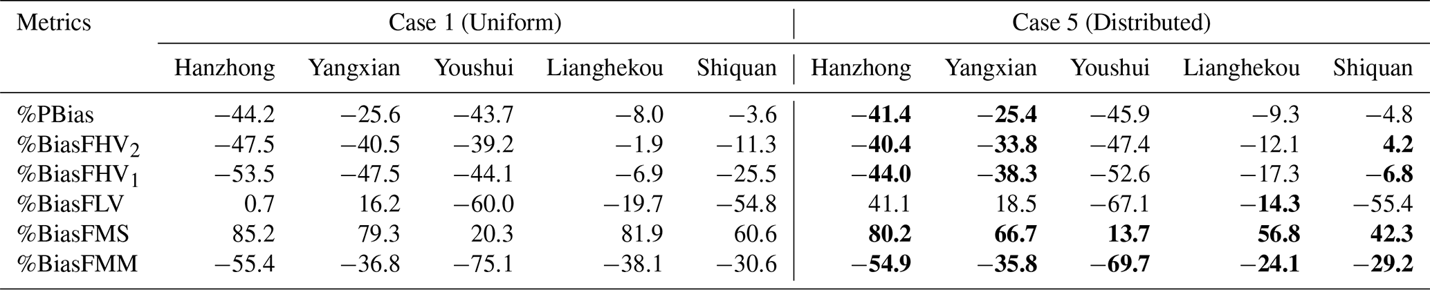
^* Note: %BiasFHV₂ and %BiasFHV₁ are defined as the bias for the high-flow segment at exceedance probabilities of 0.02 and 0.01, respectively.

Table 9 Comparison of hydrologic signature metrics during the validation period under single-gauge calibration: Case 7 versus Case 8. Bold values highlight where Case 8 outperforms Case 7.

4.2.2 Water balance simulation

We now examine the differences in simulated water balance components at the watershed scale under the enhanced model with spatially explicit parameterization. Here, four major components (i.e., surface runoff, baseflow, evaporation, and soil water storage change) in the VIC model are spatially averaged over the entire watershed and aggregated over the validation period, with soil water storage change summed in absolute terms. This allows us to derive the relative contributions of each component, which are summarized as a nested barchart in Fig. 6. A key finding in this synthesis is a marked shift in runoff partitioning from Cases 1/7 to Cases 5/8, characterized by a substantial decrease in baseflow and a concurrent, commensurate increase in surface runoff. This redistribution is consistent with, and provides a process-based explanation for, the previously noted improvement in high-flow simulation. It reveals the definitive influence of the spatially explicit parameterization scheme, which affects runoff generation processes by integrating spatial soil and terrain data into parameter estimation and provides greater flexibility in discretizing the vertical soil profile.

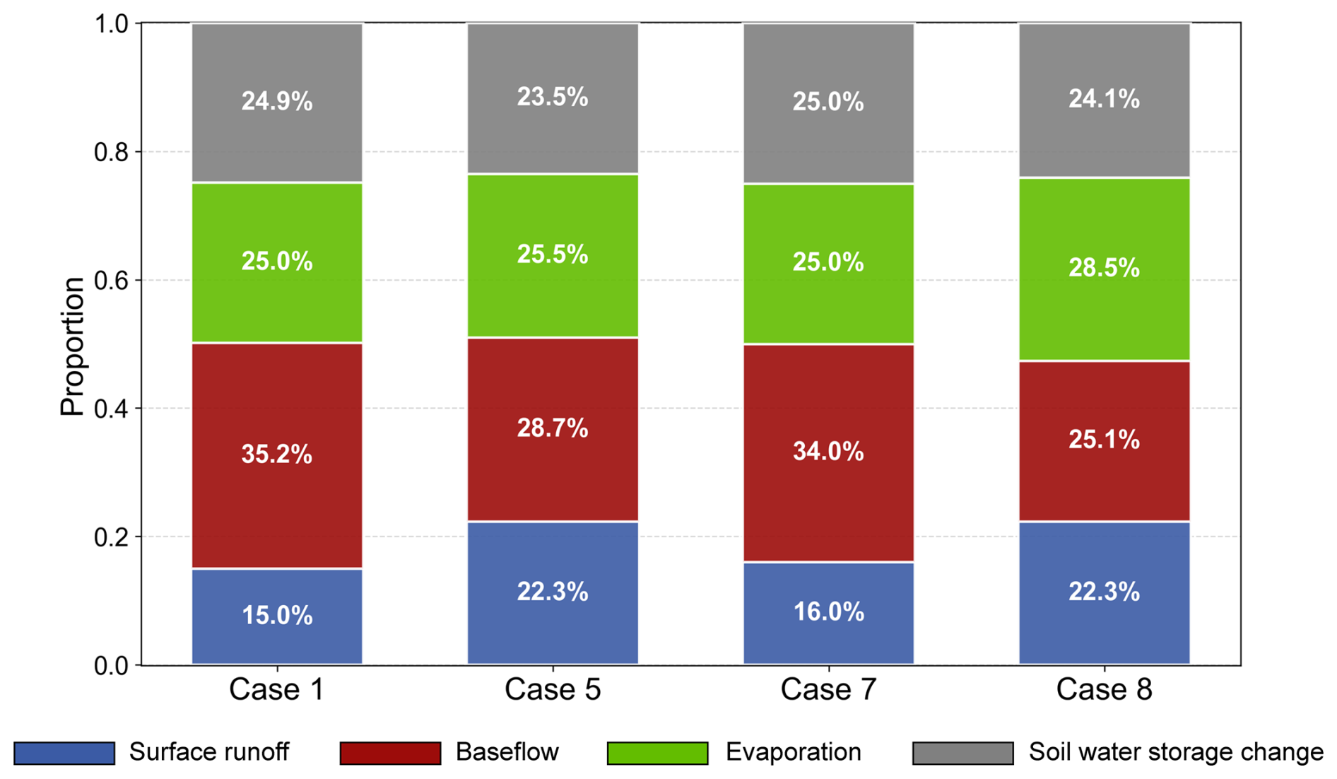
Figure 6 Relative contributions of four major water balance components for different case configurations during the validation period.

4.2.3 Spatial pattern simulation

Having identified shifts in bulk runoff partitioning, we, as a matter of course, proceed to examine their spatial manifestations. The central curiosity is the extent to which spatially explicit parameterization regulates the representation of spatial heterogeneity in hydrological processes compared to a uniform method. This leads us to examine the differences in surface runoff and baseflow between the two configurations, as shown in Fig. 7. Clearly, the improved spatial parameterization systematically increases surface runoff and decreases baseflow across the entire modelling domain, a result consistent with prior findings. More significantly, this shift exhibits a blended spatial pattern, driven by sub-basin delineation according to soil layer depths (which enhances modulation in mid- to upper-stream sub-basins), and modulated by grid-scale variations in soil and topography (which attenuate differences in the low-elevation valleys of the midstream region). We argue that this spatially refined modulation of runoff generation is beneficial, at least for simulating medium to high flows, supported by the preceding analysis.

To conclude, the spatially explicit parameterization exerts a pronounced influence on hydrological simulations, as reflected in outlet hydrographs, runoff partitioning, and spatial distributions. This enhancement significantly benefits medium-to-high flow simulations but compromises extreme low-flow accuracy. Under single-gauge calibration, the potential risk of parameter under-constraint increases, which can in turn lead to degradation in runoff simulations for non-target sub-basins, highlighting the nuanced trade-offs between model complexity and overall fidelity. The following section assesses whether spatially explicit parameterization exacerbates equifinality.

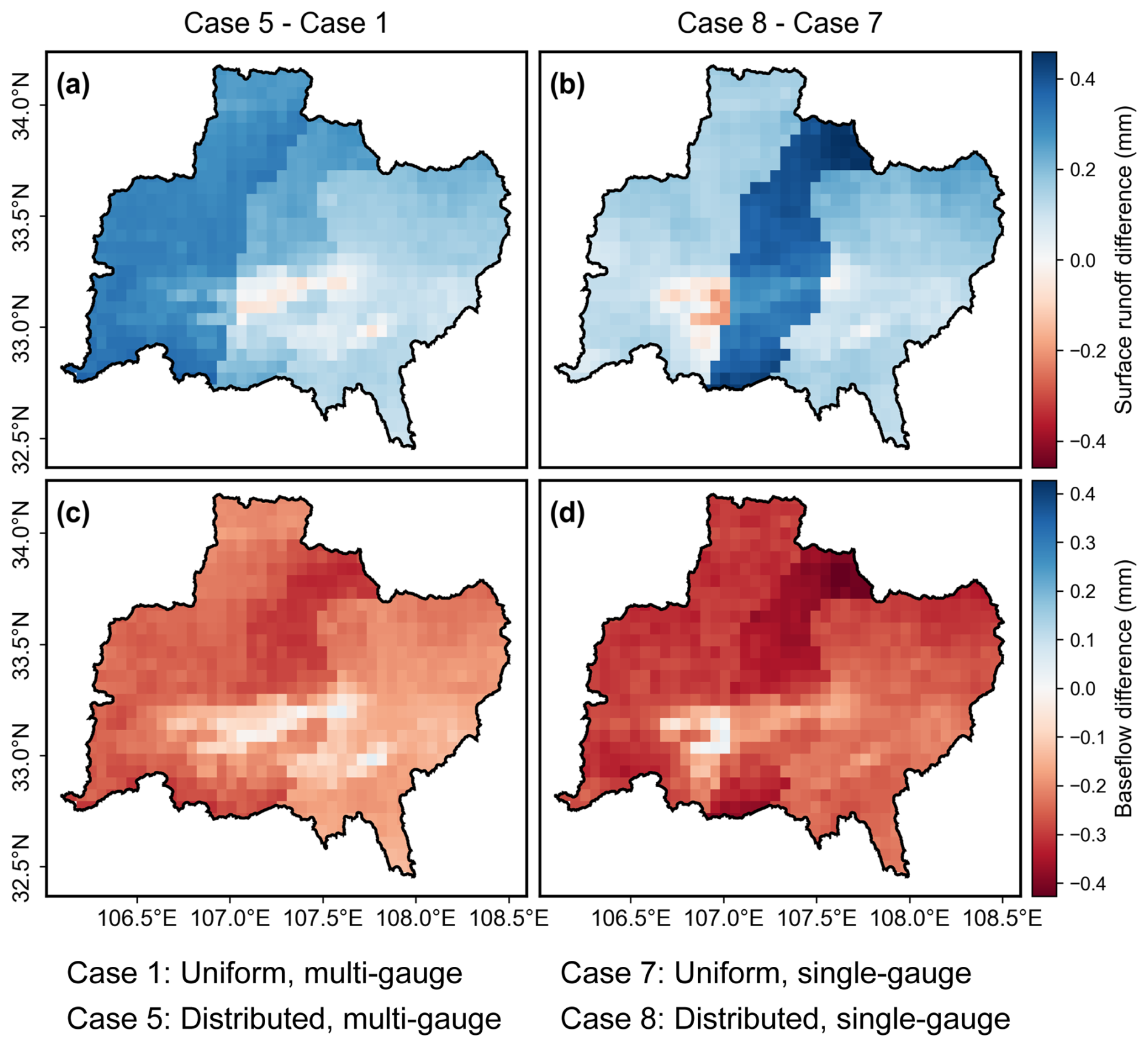
Figure 7 Spatial distribution of differences in (a, b) surface runoff and (c, d) baseflow volumes between the two parameterization schemes over the validation period. Differences are calculated as spatially explicit minus uniform parameterization.

4.3 Revealed perspectives from multi-gauge calibration

This section delves into the parameter identifiability and calibration process to determine, via a comparative analysis (Exp. 2-1 [MS-DP]: Case 5 vs. Case 8, Exp. 2-2 [MS-UP]: Case 1 vs. Case 7), whether multi-gauge calibration confers a distinct advantage over its single-site counterpart and to investigate any cross-effect with the spatially explicit parameterization.

4.3.1 Identifiability of parameters

The inverse problem of hydrological model calibration is often ill-posed due to insufficient constraints. The under-constrained condition gives rise to equifinality, where distinct parameter sets yield nearly identical model responses, thereby complicating the identification of an optimal parameter set. A particularly concerning consequence of this equifinality is the problem of “right answers for all of the wrong reasons”. This issue has prompted extensive discussion on parameter identifiability within the hydrological community (Kittel et al., 2018; Aerts et al., 2024; Talbot et al., 2025).

Parameter identifiability, simply put, refers to the ease of isolating an optimal parameter set within the parameter space. By examining the relative positions of the optimal parameters and the sampled candidate solutions across the entire calibration process within the parameter space, we can investigate how identifiability is shaped by model complexity (i.e., spatial configuration of parameters) and by the formulation of the inverse problem (i.e., the calibration setup). Our comparative analysis reveals that, in contrast to Case 7 (Fig. 8), Case 1 exhibits a more concentrated kernel density distribution, with its optimal parameters consistently located near the region of highest frequency (Fig. 9). A similar finding is also observed when comparing Case 8 to Case 5, as detailed in Figs. S4 and S5 of the Supplement. Therefore, we can reasonably conclude that multi-gauge calibration yields better-constrained solutions, leading to a significant enhancement in model parameter identifiability. From a theoretical perspective, this pattern arises from the use of globally shared free parameters (e.g., the b parameter under uniform settings and the g parameter in the MPR scheme), whose spatial compensation effects are mitigated through multi-gauge calibration (Liu et al., 2012). Furthermore, a comparison of Figs. 9 and S5 indicates a weakening in the clustering of background contours for Case 5. This weakening suggests that the spatially explicit parameterization, while enhancing spatial representational capacity, also expands the parameter set, reduces parameter identifiability, and consequently exacerbate model equifinality.

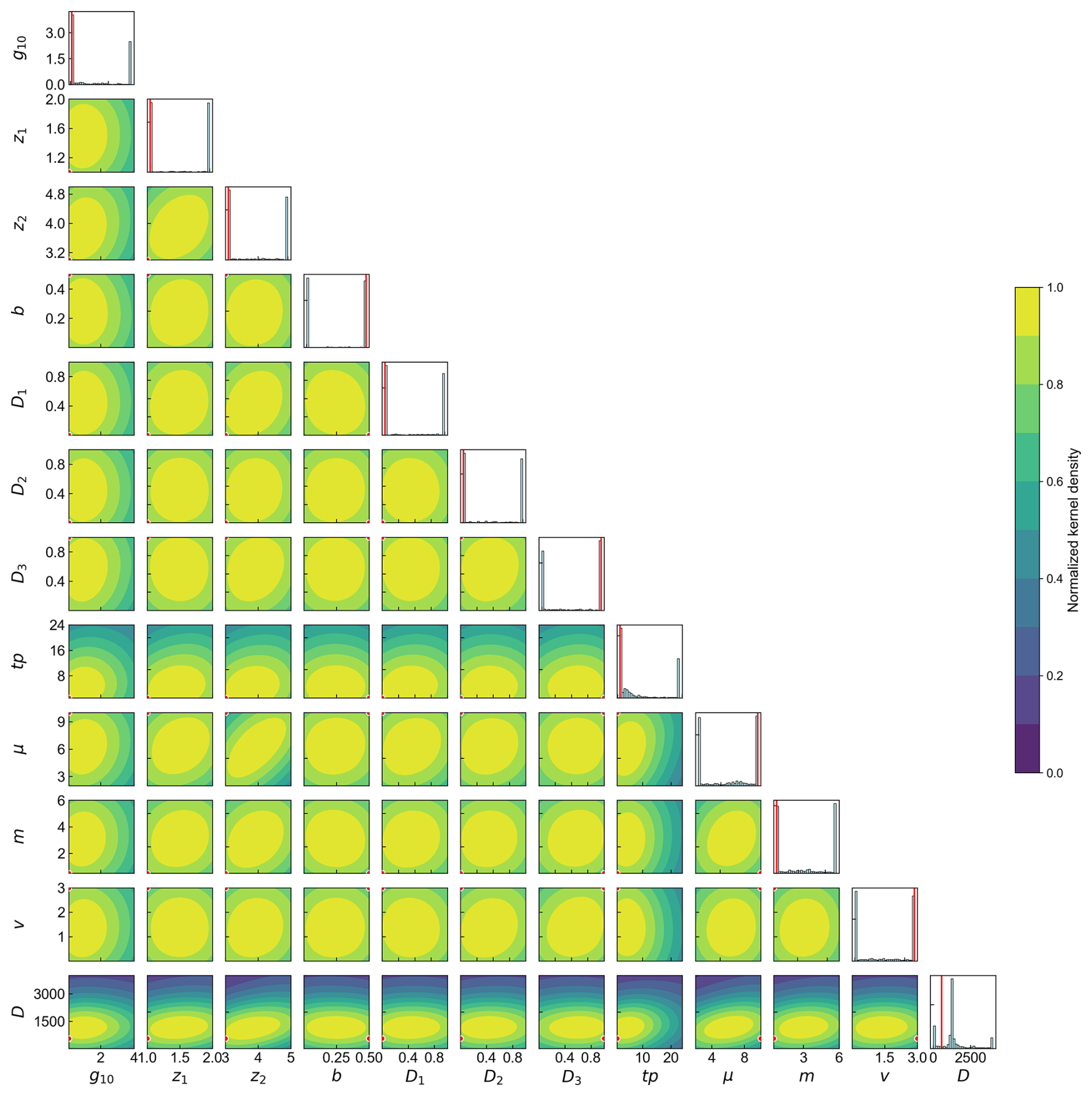
Figure 8 Post-calibration parameter distributions for Case 7. The optimal parameters are shown as red dots and lines. The background contours represent the standardized kernel density estimate derived from all candidate solutions, where yellow shading corresponds to high probability density regions. The histograms along the diagonal represent the marginal distribution of each individual parameter.

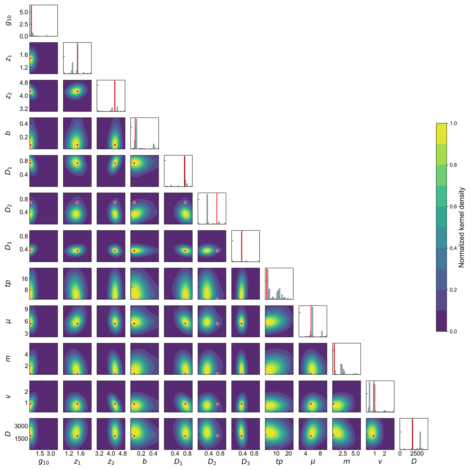
Figure 9 Post-calibration parameter distributions for Case 1, following the same visualization conventions as Fig. 8. While the overall structure is similar, Case 1 exhibits more concentrated posterior distributions and different optimal values.

4.3.2 Transferability of parameters

Multi-gauge calibration enhances parameter identifiability and mitigates equifinality by imposing joint constraints on shared parameters. This mechanism is rooted in the intrinsic hydrological connectivity among sub-basins within a closed water balance system. Physically, the hydrograph at a downstream gauge integrates contributions from multiple upstream sub-basins; conversely. upstream streamflow dynamics can be constrained – albeit implicitly – by downstream observations through the routing process. Within this context, a challenge closely aligned with Prediction in Ungauged Basins (PUB) is parameter transferability. A critical question arises: when upstream observations are unavailable, can downstream gauges provide sufficiently informative constraints to facilitate the effective transfer of parameters to ungauged upstream sub-basins?

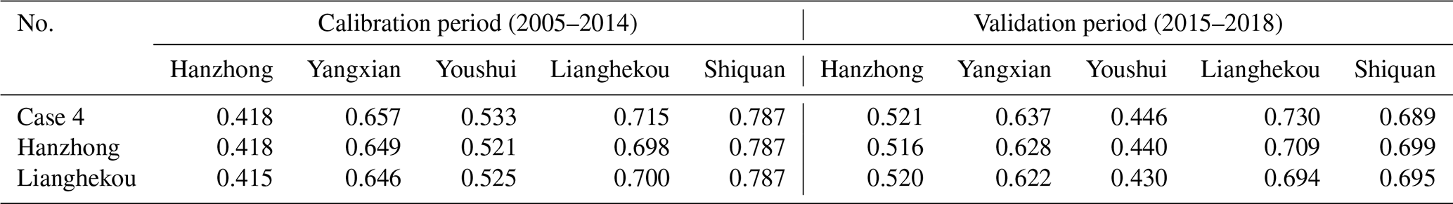
To answer this question, we established an experimental setup based on Case 4 (Table 3). Specifically, VIC and RVIC parameters were parameterized in a spatially explicit manner, while soil-layer depth parameters were maintained as spatially uniform, as only shared parameters across sub-basins are amenable to transfer. The calibration employed a leave-one-out multi-gauge strategy, optimizing streamflow KGE across four gauges while holding out the single upstream gauge for independent validation. To guarantee the robustness of our findings, parameter transferability was evaluated individually for the Hanzhong and Lianghekou sub-basins (Fig. 1).

Table 10 presents a comparison of ensemble mean KGE values for each sub-basin, contrasting the baseline Case 4 calibration with the transfer-based simulations using the five best-performing parameter sets. It is evident that, despite the absence of local upstream streamflow observations, the runoff simulation performance for the transfer targets exhibits only a marginal degradation compared to the baseline, remaining well within an acceptable range. This is further illustrated in Fig. S6, where the simulated hydrograph under the transfer scenario closely mirrors the Case 4 baseline – a consistency that becomes even more pronounced at the monthly time scale (Fig. S7). These results lead to the inference that, at least under the current model configuration, downstream gauges can provide sufficiently informative constraints to facilitate reliable runoff simulations in ungauged upstream sub-basins. This inference is further corroborated by the simulation results at the Lianghekou gauge, as shown in Figs. S8 and S9.

As a supplementary analysis, a paired t-test was conducted to compare the simulation performance at the Shiquan outlet between the Case 4 baseline and the transfer scenario, using the top 40 ranked optimization results (similar to the procedure in Table S2). The results reveal no statistically significant difference (t-statistics of 0.454 and 0.487, respectively), indicating that the current information deficiency in upstream sub-basins does not exert a significant impact on the simulations at the basin outlet. Overall, the aforementioned findings highlight the inherent advantages of multi-gauge calibration in nested basins for reducing information-gap-induced uncertainties. Furthermore, one can envision that as local observations are sequentially removed from the calibration process, the global simulation accuracy may deteriorate, potentially reaching a tipping point where the absence of a particular gauge exerts a disproportionate impact. Such a gauge would be deemed more informative in providing critical constraints for regional hydrologic modelling. A systematic investigation into this phenomenon would provide valuable insights for regional hydrologic simulation and monitoring network design, ensuring that resources are prioritized for the most strategically significant locations (Nasta et al., 2025). While such an exploration is beyond the scope of the present study, it remains a compelling direction for future research.

Table 10 Comparison of ensemble mean KGE between the baseline Case 4 calibration and the leave-one-out transfer simulations.

4.3.3 Cross-benefits of multi-gauge calibration and spatially explicit parameterization

Following the demonstrated advantages of multi-gauge calibration, we now turn to a pivotal follow-up question: what cross-benefits does spatially explicit parameterization confer, aside from its potential drawback of reduced identifiability? Addressing this is crucial for explaining the performance advantage of Case 5 over Case 1 (Table 7), despite the fact that they share the same calibration configuration and that Case 5 appears to pose greater calibration challenges (Fig. S5). Note that, from an experimental design perspective, we have grouped this section into Exp. 1-1 (UD-MG) for the sake of simplified categorization.

To answer the above question, we visualize the objective space for Cases 1 and 5 using multi-objective scatter plot matrices, as shown in Figs. 10 and 11. Interestingly, under the uniform parameter configuration (Case 1), the objectives exhibit pronounced trade-offs, manifested by continuous and convex arc-shaped Pareto fronts formed by the point clouds. In particular, gains in streamflow performance at Shiquan station degraded simulations at other sites (last row of Fig. 10). This phenomenon is consistent with our earlier finding of a compensatory effect under single-gauge calibration (Table 9), an outcome that is clearly detrimental to model realism. In contrast, when shifting to the spatially explicit parameterization in Case 5, the trade-off relationships were remarkably alleviated, accompanied by a broader dispersion of solutions in the objective space (Fig. 11), which can be interpreted as indicative of a more exhaustive calibration search that helps avoid entrapment in local optima.

Taken together, cross-benefit from spatially explicit parameterization combined with multi-gauge calibration are witnessed. This synergy indicates that enhancing spatial representation and imposing stronger constraints are mutually reinforcing. Improvements in either aspect alone exhibit clear limitations. For example, enhancing spatial representation without sufficient constraints can severely degrade parameter identifiability (as in Case 8). This provides a rationale for why, as hydrological models evolve from lumped to increasingly complex distributed formulations, parameter equifinality has gained growing attention (Wambura et al., 2018). Against this backdrop, multi-objective calibration is gradually emerging as a standard paradigm within the contemporary hydrological community. Conversely, relying solely on increased constraints while lacking adequate representation may intensify undesirable trade-offs among objectives (as in Case 1). This phenomenon is also reflected in prior literature, where studies have found that incorporating variables such as evaporation, soil moisture, or total water storage alongside streamflow in model calibration can degrade streamflow simulation performance – a typical trade-off that highlights potential structural limitations of model (Széles et al., 2020; Mei et al., 2023; Talbot et al., 2025). While existing work has largely been diagnostic in identifying this limitation, our study adopts a comparative framework (EF-SPM) to more explicitly reveal the conditions and mechanisms underlying the trade-off and cross-benefit. Building on this, we contend that the next phase of model development will undoubtedly involve deeper integration with data and an increased emphasis on realism. This requires parallel advancements in both model representation and observational constraints, culminating in a robust framework for Model-Data Infusion.

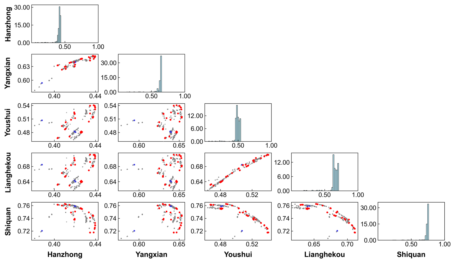
Figure 10 Objective space scatter plot matrix for Case 1. The matrix depicts the trade-offs between calibration objectives, where each axis corresponds to the Kling-Gupta Efficiency (KGE) of simulated streamflow for a sub-basin (gauge). Grey dots represent all candidate solutions from the calibration process. The initial and final Pareto fronts are highlighted in blue and red, respectively. Histograms along the diagonal show the distribution of the KGE for each individual objective.

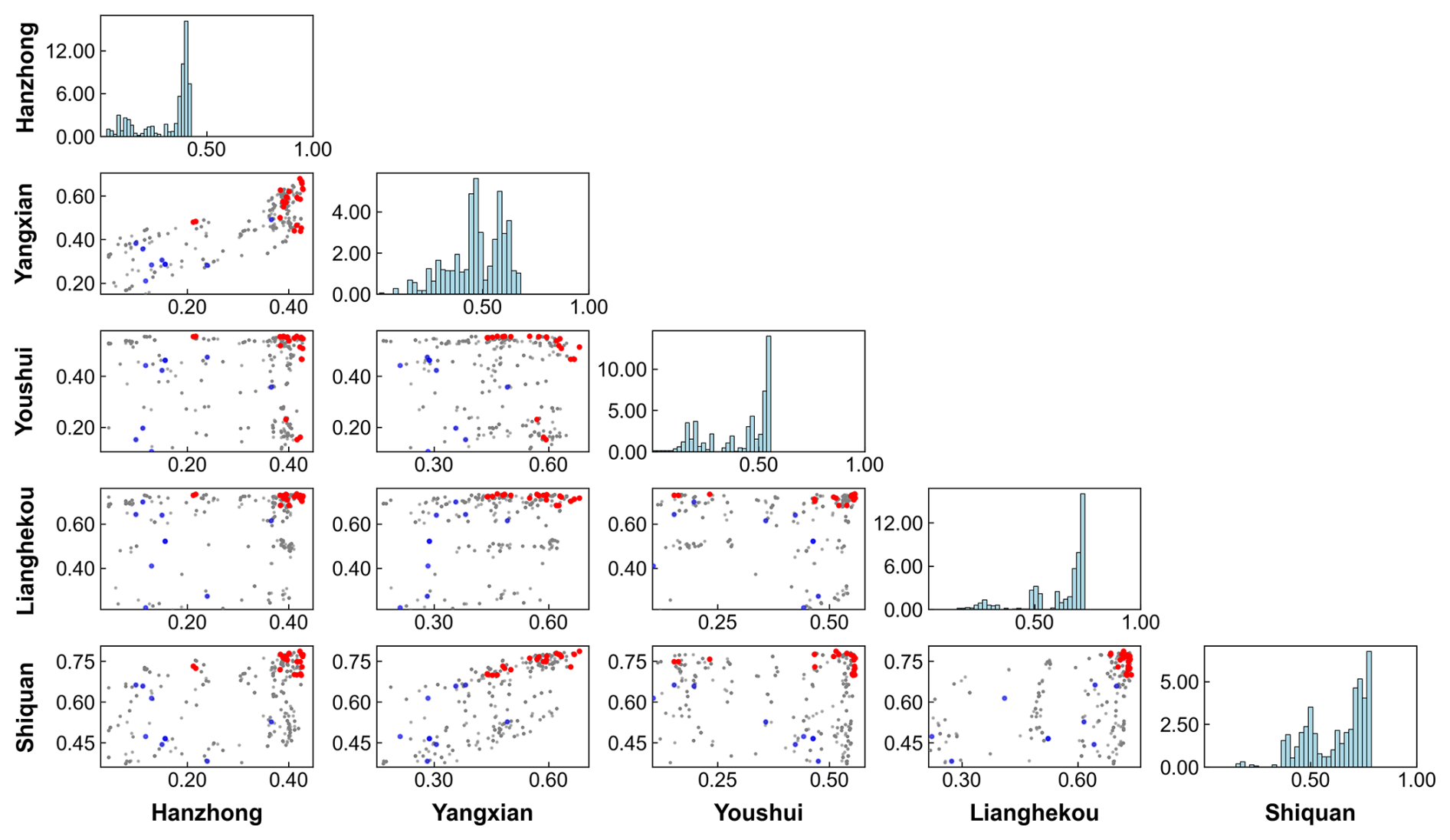
Figure 11 Objective space scatter plot matrix for Case 5, following the same visualization conventions as Fig. 10. In contrast to uniform parameter case, the trade-off relationships among objectives are substantially improved, and the solutions are more widely dispersed across the objective space.

4.4 Individual effects from additional MPR refinements

For completeness, this section investigates the individual effects of additional MPR refinements (the focus of Exp. 3) on hydrological simulations through specific case comparisons, considering two aspects respectively: soil layer depths (Exp. 3-1 [UD-MG: Depth]: Case 4 vs. Case 5) and the RVIC parameter (Exp. 3-2 [FUD-MG: RVIC]: Case 2 vs. Case 3 vs. Case 4). To ensure consistency between parameters and simulations, the top-ranked solution is adopted for analysis here rather than the ensemble values.

4.4.1 Spatial discretization of soil layer depths at sub-basin level

The spatial characterization of soil depth in the MPR-VIC modelling framework was refined via a sub-basin discretization scheme, with independent parameter sets (i.e., z₁, z₂, g₁₀) allocated to each sub-basin. From Table 7, Case 4 shows a slight advantage in the calibration period and Case 5 in the validation period, although the distinction is minimal. It is argued that the aggregated metrics encapsulate not only the effect of soil layer depths but also the influence of the jointly calibrated RVIC parameters (i.e., routing process). To disentangle these effects, analysis is focused on the contrasting runoff generation process between the two cases.

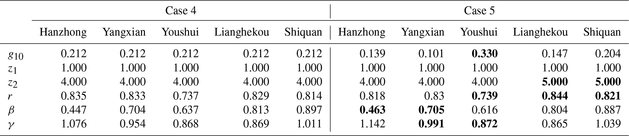
According to Fig. S10, Case 5 produces lower spatially averaged soil moisture throughout the year in the upper and middle layers compared to the Case 4, with only minor differences in runoff-related components at the basin scale. However, the heterogeneity in runoff generation resulting from the parameterization of soil layer depths is clearly evident in space. As can be observed in Fig. 12 (which shows the differences for Case 5 vs. Case 4), the middle-upper sub-basins (Hanzhong, Yangxian) experience a significant increase in surface runoff alongside a decrease in baseflow, whereas the downstream sub-basins (Youshui, Lianghekou, Shiquan) display the reverse change. This can be intuitively explained by the discrepancies in vertical discretization. In the two upper sub-basins, Case 5 maintains the same vertical layering depths (z₁, z₂) as Case 4 but applies a significantly reduced scaling factor (g₁₀), resulting in thinner soil layers (Table 11). This reduction promotes greater surface runoff and diminished baseflow, a direct impact of soil thickness on hydrological simulation that has been demonstrated in several previous studies (Gou et al., 2020; Yeste et al., 2024). As a result, the simulated mean streamflow at the two upstream stations showed distinct improvement, with the β component of the KGE increasing from 0.447 and 0.704 to 0.463 and 0.705, respectively. For the Youshui sub-basin, the substantially increase in scaling factor reduced both surface runoff and baseflow, owing to the enhanced storage capacity of the deepened third layer. The behaviour of the downstream stations differs most significantly between Case 5 and Case 4. Although the total soil thickness is reduced in Case 5, the change in z₂ reallocates the depth distribution, yielding a relatively thicker middle layer (d₂) and a thinner third layer (d₃). Consequently, surface runoff decreases whereas baseflow increases, which contributes to an improved overall correlation (γ) in the streamflow time series (Table 11).

Several limitations of the current analysis should be noted. First, the differences in vertical soil layering affect not only the layer thicknesses but also the aggregated soil properties (Fig. 2). This, in turn, leads to variations in parameters such as D₁, D₂, and D₃, as these parameters depend on the layer-specific soil hydraulic properties (e.g., K_s). Nevertheless, these secondary effects are not analysed further through controlled variable comparisons, owing to their intricately coupled nature. Second, the calibrated results for Case 5 are not considered the definitive optimum, as the calibration was limited to only 40 trials due to available computational resources. Further optimization may yield more distinct vertical layering configurations, which we reserve for future investigation. Finally, we avoid basing the superiority of Case 4 or Case 5 exclusively on outlet flow performance. Such a single metric is inadequate because it masks not only the equifinality inherent in the joint calibration of VIC parameters, but also the complex interdependencies within the river network – where improvements in upstream simulations may compromise downstream accuracy. Nevertheless, the analysis above provides a clear indication that Case 5 exhibits improved spatial representativeness and flexibility compared to Case 4 at the sub-basin scale. In the absence of strong prior knowledge, discretization of soil layer depths at the grid-cell scale is nearly infeasible. A more pragmatic path forward, however, would be to cluster grid cells based on salient landscape attributes (e.g., elevation), an approach which we intend to explore in future work.

A further point that merits discussion is that current spatial parameter estimation methods (e.g., MPR) rely heavily on soil information. This reliance arises because many distributed hydrological models follow the FH69 blueprint and adopt a bottom-up modelling paradigm in which the Darcy-Richards equations are embedded in the representation of runoff-generation processes, thereby providing the basis for estimating model parameters from soil information (Freeze and Harlan, 1969). However, such a widely adopted practice may involve substantial uncertainty and several assumptions that are not readily apparent. For example, the development of transfer functions is associated with considerable subjective prior uncertainty, given that many field measurements are often limited in sample size and by insufficient representativeness in terms of vertical depth or spatial extent. In addition, scale effects arising from the extrapolation of microscale relationships to larger scales constitute an important source of uncertainty. Furthermore, some soil parameters may still lack a priori information and can only be determined through calibration, which may compromise model realism. A pertinent example in this study is soil depth: under spatially uniform parameterization, soil depth clearly cannot fully represent the differences in runoff generation processes among sub-basins in a physically realistic manner (Fig. 12). On the other hand, the role of ecosystems may be substantially underestimated in current hydrological modelling. In the VIC model used here, vegetation is represented only through simplified descriptors such as LULC, LAI, and NDVI, while the root zone is treated even more simply through a priori vertical distributions prescribed by LULC-based lookup tables, which may compromise model realism. Increasing data availability creates new opportunities to more explicit incorporation of ecosystem constraints into hydrological modelling, for example through the integration of spatially distributed root-zone information, with the potential to further improve model physical realism (Gao et al., 2024). The above discussion echoes the view advanced by Gao et al. (2023) that soils may overrated in hydrology, and perhaps even more so in hydrological modelling. Although the foundations of bottom-up modelling may appear deeply entrenched, their critical revision and improvement remain an important direction for continued development in the hydrological community. In this context, the present study contributes by highlighting the importance of the combined application of spatially explicit parameterization and multi-gauge calibration.

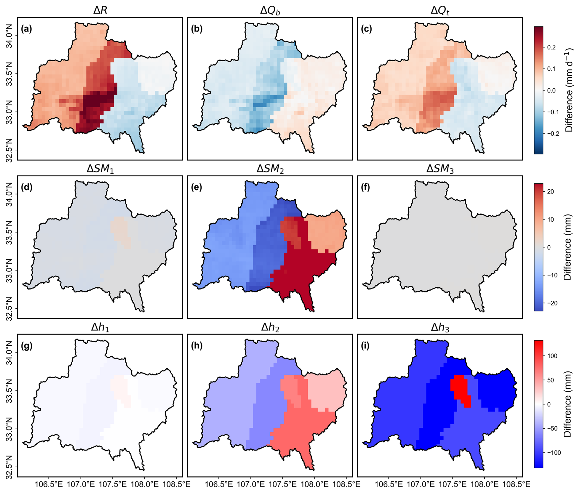
Figure 12 Spatial distribution of differences in long-term mean simulated variables during the validation period and soil layer depths between Case 4 and Case 5. Differences are shown for (a–c) surface runoff (R), baseflow (Q_b), and total runoff (Q_t), and (d–f) soil moisture in layers 1–3 (SM₁, SM₂, SM₃), respectively. The bottom row presents the corresponding differences in the calibrated soil layer depths: (g–i) Depths differences for soil layers 1–3 (Δh₁, Δh₂, Δh₃). Positive values indicate higher magnitudes in Case 5 relative to Case 4.

Table 11 Comparison of soil vertical layering parameters and signature metrics during the validation period: Case 4 versus Case 5. Bold values indicate an increase in the parameter value or a performance improvement for Case 5 relative to Case 4.

4.4.2 Spatialization scheme for RVIC parameters at the grid level

Cases 3, 2, and 4 – defined by constant, uniform, and distributed parameters, respectively – form a gradient of increasing complexity in RVIC model parameterization. We assess the potential benefits corresponding to this parametric refinement. To factor out the effect of runoff generation, all three cases were run with an identical set of runoff generation parameters from the simplest Case 3 configuration, altering only the runoff concentration parameters. Their performance was then evaluated. Interestingly, this approach yielded results that diverged from the established benchmarks (Table 7). As shown in Table 12, a consistent performance ranking was observed across all sub-basins, with Case 4 demonstrating superior performance, followed by Case 3 and then Case 2. This finding provides two key insights into the model behaviour. First, it highlights the effect of joint calibration of runoff generation and concentration parameters. While a calibratable mechanism may underperform a fixed-parameter setup in isolation, it offers greater flexibility. When jointly calibrated with runoff generation parameters, its performance can surpass that of the fixed-parameter mechanism (as in Table 7). The importance of joint (i.e., hydrological and routing) parameter search strategies has also been emphasized in previous research (Cortés-Salazar et al., 2023). Second, the grid-level RVIC spatial parameterization scheme based on predefined transfer functions demonstrates a clear advantage, despite incorporating only minimal river network information (i.e., accumulation area and flow distance). To test for robustness, the experiment was repeated using the runoff generation parameters of the most complex Case 4; this repetition confirmed the consistency of the findings (Table S2).

For a more detailed analysis of the inter-case differences, a comparison of their streamflow simulation residuals was conducted (Fig. 13). The first observation is that the residual scatter points for Cases 2 and 3 cluster around the 1:1 line, indicating no significant difference in their simulation residuals. This suggests that, by default, using the officially recommended RVIC values is a viable approach. In contrast, a comparison between Case 2 and Case 4 reveals a clear difference. Case 4 demonstrates reduced underestimation of high flows (Quadrant III), suggesting better peak performance, at the cost of overestimating medium and low flows (Quadrant I). This behaviour is more pronounced at the Shiquan outlet station. Likewise, the robustness of these findings was further confirmed through a repeated experiment based on the runoff generation parameters of Case 4, as shown in Fig. S11.

In many previous hydrological modelling applications, researchers have often focused considerable effort on improving the representation and calibration of runoff generation processes (Wang et al., 2022), while seemingly paying less attention to runoff concentration mechanisms. However, the findings of this study suggest that even minimal refinements to the spatial parametrization of the RVIC model – such as those implemented here – can lead to significant improvements in streamflow simulation, particularly for peak flows which are of critical concern. It should be acknowledged that the transfer functions employed in this study are relatively simple, incorporating only limited river network information (i.e., accumulation area and flow distance). Future work could therefore explore more sophisticated parametrizations in this direction, for example, by integrating hydraulic characteristics such as channel geometry and roughness into the transfer function, or by developing regionalized transfer functions based on machine learning techniques (Kupzig et al., 2024; Farahani et al., 2025; Ali et al., 2025). A meaningful insight emerging from this work for the development of next-generation distributed hydrological models is that advances in model parametrization should be pursued in tandem with calibration strategies that explicitly account for the resulting changes in parameter identifiability. This consideration applies equally to future developments that seek to enhance the complexity of runoff routing mechanisms.

Table 12 Performance comparison of Cases 3, 2, and 4 during the validation period, with runoff generation parameters held constant as in Case 3. Performance is quantified by the KGE metrics, with the best value for each sub-basin shown in bold.

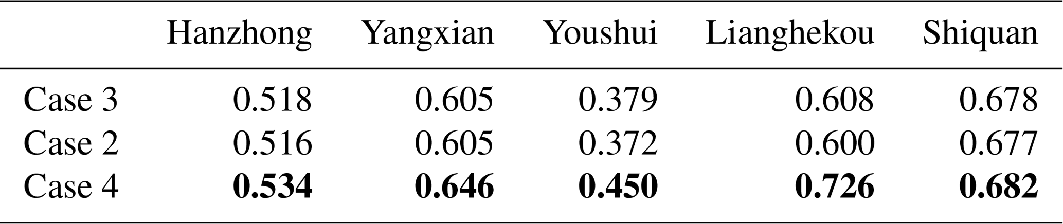
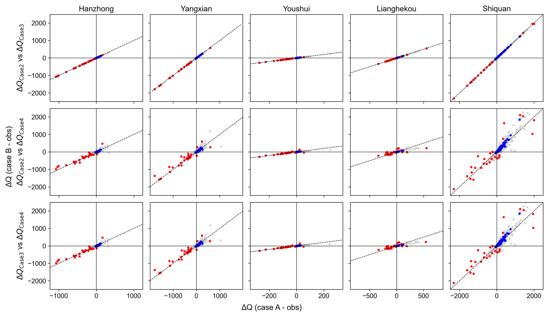
Figure 13 Scatter plots of simulated streamflow residuals (ΔQ) for Cases 3, 2, and 4 during the validation period, using the runoff generation parameters from Case 3. Red and blue dots represent high flows (exceedance probability < 2 %) and low flows (exceedance probability > 70 %), respectively. The dashed line indicates the 1:1 line.

5 Conclusion

This study evaluated the benefits of spatially explicit parameterization and multi-gauge calibration for improving model realism and further disentangled their respective contributions, as well as their cross-benefits, through a dedicated experimental framework, termed EF-SPM. Built on the new-generation Variable Infiltration Capacity (VIC-5) model integrated with the multiscale parameter regionalization technique, the framework was applied to the representative nested Upper Han River Basin (UHRB) through intensive calibration experiments. Our key findings and conclusions are given in the following.

Both spatially explicit parameterization and multi-gauge strategy led to consistent gains in model performance across all sub-basins. Spatially explicit parameterization strategy mainly improved simulations under moderate-flow and high-flow conditions and substantially enhanced peak-flow representation, as indicated by 18 % improvement in %BiasFHV₁ at the main outlet; however, low-flow performance deteriorated. The multi-gauge calibration strategy offers a distinct advantage over its single-gauge counterpart by significantly enhancing parameter identifiability, demonstrated in the more clustered distribution of optimal and sampled candidate solutions within the parameter space. Furthermore, this strategy effectively reduces information-gap-induced uncertainties, thereby allowing for robust parameter transfer to ungauged upstream sub-basin.

The combined use of the two strategies yielded clear cross-benefits relative to their separate use. On the one hand, spatially explicit parameterization increases parameter dimensionality and thus poses a potential risk of reduced identifiability, whereas multi-gauge calibration strengthens observational constraints that help mitigate this issue. On the other hand, under spatially uniform parameterization, multi-gauge calibration appears to be subject to an optimization ceiling, manifested by pronounced trade-offs among gauge-specific objectives in the multidimensional objective space and by the formation of continuous, convex, arc-shaped Pareto fronts. By introducing spatially explicit parameterization, the feasible solution space is expanded, thereby raising the upper bound of achievable simulation accuracy.

Collectively, our findings suggest that enhancements in spatial representation and the strengthening of calibration constraints should be pursued in parallel during the model development. Focusing on either aspect in isolation is unlikely to produce genuinely reliable improvements and may result in right results for the wrong reasons. Looking ahead, continued advances in observational technologies and computational capacity are likely to move hydrological modelling towards a Model-Data Infusion framework, with the integration of increasingly informative data into the modelling process representing a shared direction for improving model realism.