A Robust Calibration and Evaluation Framework for Dynamic Catchment Characteristics in Hydrological Modeling

Hydrological models often face challenges in accurately simulating hydrological processes within dynamic catchments due to simplifications of model structure. In a dynamic catchment where hydrological processes exhibit significant intra-annual or inter-annual variability, accurately capturing dynamic behaviours across different flow regimes is still challenging for models. To address these challenges, this study investigates calibration issues in dynamic catchments with a focus on two key aspects: the influence of objective function design on flow-phase-specific performance, and the limitations of sub-period calibration with dynamic parameters. Seven calibration experiments were designed to explore issues related to time-invariant parameters, objective function configurations, parameter correlations, dimensionality in global optimization, and abrupt parameter shifts. The experiments were conducted using the MOPEX dataset, which includes 219 basins across the United States, and were evaluated based on performance metrics, as well as state variables and fluxes. Among all calibration schemes, sub-period calibration with dynamic parameters exhibited the most reliable performance. Static parameter approaches often averaged catchment responses and poorly represented extreme flows, whereas enabling temporal variability to only a subset of parameters yielded limited improvement. In contrast, multi-parameter dynamic schemes significantly improved NSE and LNSE values and enhanced parameter transferability across flow phases, where the high-dimensional calibration strategy balanced dynamic adaptability with physical consistency, while the parallel calibration maintained accuracy through gradual parameter transitions despite higher variability in some catchments. This study demonstrates that sub-period calibration with dynamic catchment characteristics outperforms traditional static parameters by effectively capturing flow-regime variability and sustaining robust performance under changing catchment conditions, offering a generalizable solution for simulating hydrological processes in dynamic catchments.

1 Introduction

Hydrological models serve as essential tools in water management, supporting tasks such as runoff projection, disaster warning, and water-resource planning (Shao et al., 2023; Shrestha et al., 2021; Razavi et al., 2025). These models conceptualize hydrological processes with physically based parameters and state variables, enabling transparent simulations and process-informed diagnostic analysis of the catchment. However, limited understanding of the mechanisms underlying seasonal climate patterns, vegetation dynamics, and water storage variability has led existing model structures to rely on simplified representations of hydrological processes and steady-state assumptions (i.e., time-invariant parameters). Such assumptions only partially capture the dynamic catchment characteristics (Deng et al., 2016; Wang et al., 2022b; Wen et al., 2021). A dynamic catchment is defined as one in which hydrological processes exhibit significant intra-annual or inter-annual variability, making their simulation particularly challenging. Dynamic catchment characteristics denote the time-varying states of a catchment that describe the temporal evolution of hydrological processes, such as precipitation seasonality and changes in vegetation cover under significant human disturbances. As a result, models tend to capture only the “average” behaviour of catchments, often at the cost of reduced accuracy in high- or low-flow phases (Longyang and Zeng, 2023; Yoshida et al., 2022). Understanding, modelling, and predicting dynamic hydrological processes with greater realism remain significant challenges in hydrological sciences (Bouaziz et al., 2022).

A key challenge in modelling catchments with dynamic variability lies in how to adapt the model to accurately reflect time-varying hydrological responses. Calibration aims to adjust model parameters using local observations, thereby tailoring a general model structure to the hydrological responses of a specific catchment. This process typically involves the definition of objective functions and the systematic exploration of parameter space. The mathematical form of the objective function determines which aspects of model performance are emphasized, such as the accuracy of peak flows or the representation of overall water balance (Gupta et al., 2009; Fauer et al., 2021). In catchments with strong dynamics, however, the calibrated parameter sets may reflect not only the actual catchment behaviour but also implicit structural limitations and assumptions about boundary conditions. Consequently, the calibrated parameters often reflect trade-offs shaped by the objective function and model structure, leading to an averaged performance across flow phases (such as extreme high flow, high flow, middle flow, low flow, and extreme low flow).

One common strategy to improve model performance under structural limitations is to refine the configuration of the objective function to better emphasize key hydrological processes. Such a challenge is not unique to dynamic catchments, but represents a general issue in hydrological model calibration. Traditional calibration of hydrological models typically employs global evaluation metrics and time-constant parameters, focusing on the model's overall performance. However, this approach might average hydrological responses and fail to ensure accurate simulations across various flow phases and observational periods. In critical runoff events like floods and droughts, this static approach may fail to capture the dynamic catchment characteristics of hydrological processes, underscoring the need for more flexible calibration methods (Martel et al., 2025; Clark et al., 2021). In dynamic catchments, such limitations become more evident as hydrological responses vary across seasons or years. To alleviate these limitations, various calibration strategies have been proposed to incorporate dynamic catchment characteristics. One method involves revising the objective function based on selected evaluation criteria to improve model performance (Araya et al., 2023; Ji et al., 2023). Calibrations using multi-objective optimization algorithms better highlight different flow phases, but face potential challenges such as increased computational complexity, sensitivity to parameter settings, and slower convergence with more objective functions (Song et al., 2024; Carletti et al., 2022). Alternative approaches, like multi-weighted objective functions, can improve the simulation accuracy of specific time and flow phases. While these methods enhanced different flow phases and water balance, they may not effectively address structural deficiencies and cannot fundamentally enhance the model's overall performance (Lin et al., 2024; Anderson and Radić, 2022).

Another strategy involves the use of dynamic parameters in hydrological models. A dynamic parameter is defined as a model parameter that varies across sub-periods rather than remaining fixed over the entire simulation period. Sub-periods are segments of the simulation period characterized by relatively homogeneous hydrological conditions, which are typically identified through clustering of the time series. The implementation of dynamic parameters addresses structural limitations of models and improves predictive performance across the full range of hydrological processes, rather than being restricted to specific flow regimes or periods (Zhang and Liu, 2021; Krapu and Borsuk, 2022). Recent studies have significantly advanced hydrological simulations by integrating the dynamic catchment characteristics. Clustering based on catchment characteristics, such as precipitation, evapotranspiration, and soil moisture, facilitates the clustering of dynamic hydrological processes into distinct sub-periods (Acuña Espinoza et al., 2024; Lakshmi and Sudheer, 2021). Wei et al. (2021) further broadened this perspective by highlighting the hydrological processes that arise from the interplay of various factors, including meteorological conditions, surface characteristics, and anthropogenic interference. This interaction among water balance components, such as soil, vegetation, and topography, exhibits temporal variability, which ideally should be captured by process-driven hydrologic simulation models. These changes need to be taken into account through model parameters (Wi and Steinschneider, 2022; Reichert et al., 2021). Zhang and Liu (2021) suggested that temporal variations in parameters reflect the evolving environment. However, some fundamental problems still need to be addressed before applying the dynamic parameters. Sub-period calibration with dynamic parameters involves the hydrological model structure, global optimization, physical mechanisms of dynamic catchment characteristics, as well as complex relationships between the parameters, state variables, and fluxes.

To address the model deficiencies and improve simulation across all flow regimes, it is imperative to re-examine the time-varying information in historical hydrological and meteorological data, extract dynamic catchment characteristics, and address the variation in calibration. This study investigates calibration challenges in dynamic catchments and proposes a structured framework to address two major issues: the influence of objective function design on flow-phase-specific performance, and the limitations of sub-period calibration with dynamic parameters. Seven experiments are developed to systematically evaluate these aspects. Experiments 1–3 focus on the effects of time-invariant parameters and various objective function configurations. Experiments 4–7 explore issues in dynamic parameter calibration, such as parameter correlation, dimensionality, and state transitions. Model performance is assessed through multiple metrics and internal diagnostics across 219 MOPEX catchments.

2 Study area

The Model Parameter Estimation Experiment (MOPEX) is an international project aimed at developing enhanced techniques for a priori estimation of parameters in hydrologic models and land surface parameterization schemes of weather and climate models (Duan et al., 2006). A comprehensive MOPEX database has been developed that contains historical hydrometeorological data and land-surface characteristics data for numerous hydrological catchments in the United States (US) and other countries. This study utilizes the dataset from 219 catchments spatially distributed across the contiguous US (Fig. 1). Rigorous screening criteria were applied to ensure the acquisition of high-quality data. The screening process involved three key considerations: (1) no missing or non-physical data throughout the study period; (2) minimal interference from anthropogenic influences in both temporal and spatial dimensions; and (3) a large spatial distribution scale of the selected catchments, including diverse meteorological and underlying surface conditions. The dataset for selected catchments includes the hydrometeorological forcing data, land-surface data, and streamflow data, covering the period from 1983 to 2000. Hydrometeorological data includes daily precipitation data (P), temperature data (T), and streamflow (Q) provided by the MOPEX dataset, as well as potential evaporation data (PE) calculated by the Hamon model (McCabe et al., 2015). The Normalized Difference Vegetation Index (NDVI) was used as one of the land-surface indicators to represent the vegetation coverage of the catchments, which had a spatial resolution of 8 km and a temporal resolution of half-monthly intervals (Tucker et al., 2010). Based on these criteria, a total of 219 catchments were selected (Fig. 1), spanning a wide range of hydrological and meteorological characteristics, making them ideal for testing various model structures under diverse conditions (Duan et al., 2006).

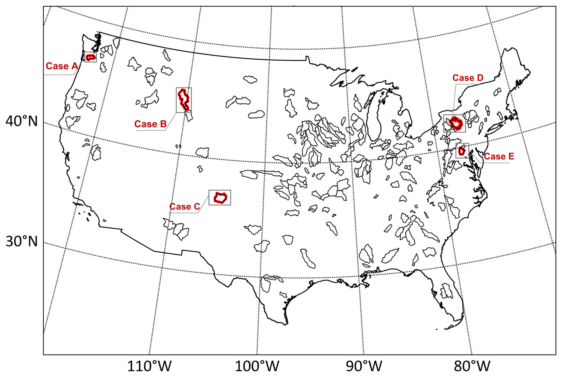
Figure 1 Location map of the catchments used in this study, where cases A, B, C, D, and E correspond to catchments 12027500, 6192500, 7211500, 1643000, and 1531000 (from west to east) are highlighted with red outlines for reference.

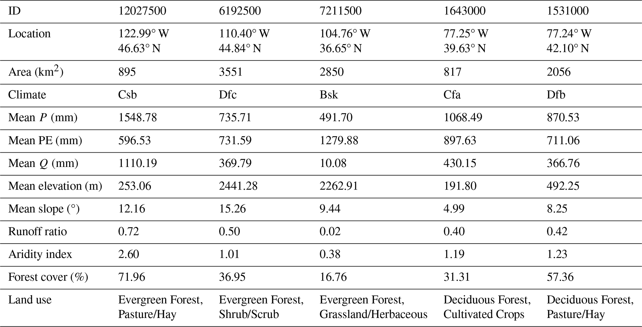
In addition to the large-sample analysis of the MOPEX dataset, five representative catchments, Case A (12027500), Case B (6192500), Case C (7211500), Case D (1643000), Case E (1531000), are analyzed in more detail as case studies. These catchments encompass a variety of Köppen climate classifications and different dominant dynamic catchment characteristics, facilitating comparison of calibration strategies and evaluation of their robustness under diverse hydroclimatic conditions. Their locations and characteristics are listed in Table 1 and will be analyzed in depth in the subsequent sections.

Table 1 Summary of catchment characteristics for study cases.

3 Methods

Hydrological processes within catchments commonly exhibit significant annual and inter-annual variability. However, conventional hydrological models often fail to capture these temporal dynamics due to structural simplifications, resulting in averaged responses and reduced simulation accuracy. To address these limitations and improve model performance across different flow phases, this study investigates two strategies: (1) refining the configuration of objective functions during calibration to enhance sensitivity to temporal variations; and (2) integrating dynamic catchment characteristics into the modelling framework through dynamic parameterization, while systematically investigating the associated calibration challenges. This study aims to evaluate the effectiveness and limitations of various calibration strategies under dynamic catchment conditions and to develop a robust calibration framework for catchments with temporal dynamics.

3.1 Hydrological models

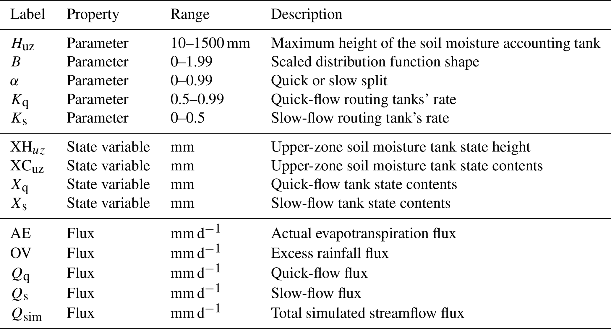
The investigated strategies involve only parameter configuration and calibration procedures, without requiring structural modifications to the hydrological model. Such strategies are applicable to lumped, semi-distributed, and fully distributed models, including both conceptual and physically based types. To evaluate the applicability of different calibration strategies under dynamic catchment conditions, the simple conceptual hydrological model HYMOD (Hydrological MODel) (Moore, 1985) is employed. HYMOD is characterized by a parsimonious structure with five parameters, low input requirements, and empirically interpretable physical meaning. It has been widely applied in streamflow prediction across America and other regions (Vrugt et al., 2003; Wagener et al., 2001). To improve performance in snow-affected regions, a degree-day model is incorporated to represent snowmelt processes (Sect. S1.6 in the Supplement) (Wang et al., 2022a). HYMOD serves as a representative model for conceptual validation and mechanism analysis, rather than constraining the applicability of the proposed framework. To further assess cross-model generalizability, additional comparisons between conventional calibration and dynamic calibration are conducted using the semi-distributed TOPMODEL and the GR4J model, as presented in Sect. S4. The structure and configuration of the HYMOD model are presented in Sect. S1.7, with detailed information on model parameters, state variables, and fluxes provided in Table 2.

Table 2 HYMOD model parameters, state variables, and fluxes (Vrugt et al., 2003; Wagener et al., 2001).

3.2 Clustering hydrological processes

Sub-period calibration provides a practical means of linking dynamic catchment characteristics with hydrological models. In sub-period calibration, the simulation period is clustered into multiple sub-periods characterized by relatively homogeneous hydrological conditions, allowing dynamic parameters to better reflect temporal variations in catchment behaviour across different streamflow regimes (Zhang and Liu, 2021). In this study, the clustering of sub-periods is guided by temporal variations in key hydrometeorological and land-surface variables. The methodological framework consists of three key steps: (1) constructing a dynamic catchment characteristic index system to describe catchment states; (2) extracting dynamic catchment characteristics through screening and dimensionality reduction; and (3) applying unsupervised clustering to cluster the time series into sub-periods with similar hydrological processes for subsequent sub-period calibration.

3.2.1 Describing dynamic catchment characteristics

To characterize the temporal dynamics of catchment behaviour, a dynamic catchment characteristic index system comprising a climatic subsystem and a land-surface subsystem is constructed to represent the time-varying states of the catchment. The climatic subsystem includes core hydrometeorological variables such as precipitation (P), temperature (T), and potential evapotranspiration (PE), along with corresponding extreme climatic indicators. The land-surface subsystem reflects evolving surface conditions through indicators such as antecedent runoff, runoff coefficient, and the normalized difference vegetation index (NDVI). All indicators are sampled using a moving window approach, with the optimal window length determined through a time-windowed Bayesian inference framework based on predictive log-score (PLS) performance (Hsueh et al., 2024). The framework is designed to preserve long-term trend signals, suppress short-term high-frequency noise, and improve the stability and robustness of dynamic catchment characteristic extraction.

3.2.2 Extracting dynamic catchment characteristics

Not all indicators exhibit significant dynamic catchment variability; therefore, filtering irrelevant or redundant variables is essential to retain meaningful catchment dynamics. A threshold-based screening is applied to identify variables exhibiting significant seasonality, retaining only relevant subsystems and forming an initial pool of candidate indicators (see Sect. S2.1 for detailed criteria). The Maximal Information Coefficient (MIC) is then employed to quantify linear and nonlinear associations between candidate indicators and streamflow, ensuring hydrological relevance. To mitigate multicollinearity and reduce dimensionality, Principal Component Analysis (PCA) is performed, with the first two principal components retained for clustering. This multi-step filtering and reduction procedure ensures robust extraction of dynamic catchment characteristics and provides a solid basis for sub-period clustering according to hydrological similarity.

3.2.3 Clustering hydrological processes

Based on the extracted dynamic catchment characteristics, the time series is clustered into distinct sub-periods using the unsupervised Fuzzy C-Means (FCM) clustering algorithm. The optimal number of clusters is determined through a combination of clustering validity indicators, including the Partition Coefficient (SC), Separation Index (S), and Xie–Beni (XB) index, which collectively assess clustering compactness and separation. In addition, the elbow method is employed as a supplementary diagnostic to identify the inflection point beyond which further increases in cluster number yield diminishing returns. Clustering is performed in the principal component space, enabling effective capture of structural patterns in catchment dynamics. The resulting sub-periods provide a robust foundation for integrating dynamic parameters into hydrological models.

In addition, the sub-period clustering is developed exclusively using data from the calibration period. To independently evaluate the generalization capability and robustness of the model under unseen conditions, no model training or parameter adjustment is performed during the evaluation period.

3.3 Calibration experiments

To systematically evaluate how calibration strategies capture catchment dynamics and improve the simulation of diverse flow regimes, a diagnostic framework comprising seven calibration strategies is developed. These experiments sequentially address key challenges in representing time-varying hydrological behaviour, with a focus on objective function design and time-varying parameterization (Fig. 2).

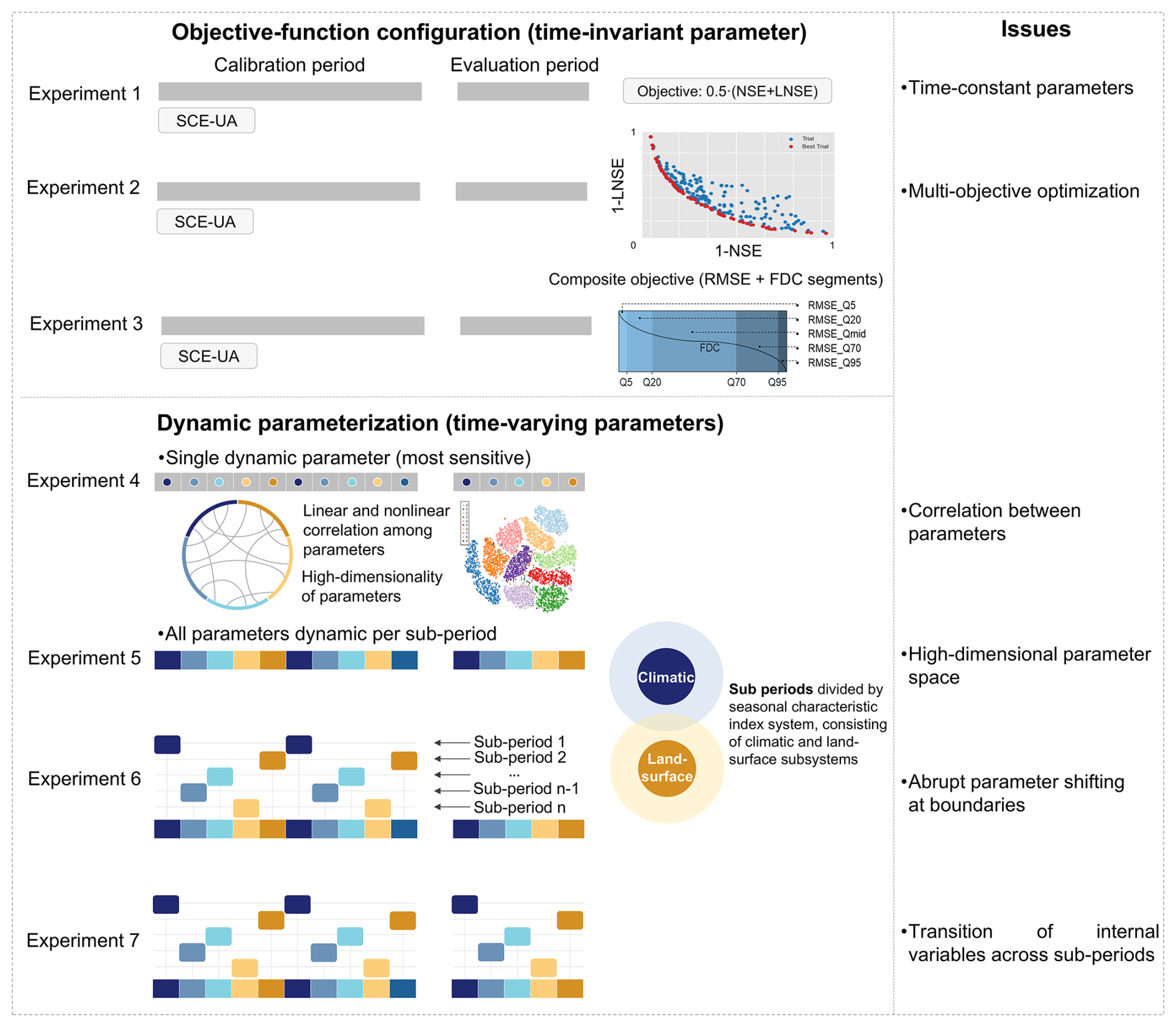
Figure 2 Schematic illustration of the seven calibration experiments. The colour bands represent state variables and fluxes, which are continuously transferred within the same period. In Experiments 1, 2, and 3, the parameters are time-invariant, but the experiments differ in their objective function configurations. Conversely, experiments 4, 5, and 6 maintain a consistent objective function, but vary the parameters across different experiments. In Experiment 4, the dynamics of only the specific parameter are operated, and the other fixed parameters are optimized simultaneously. In Experiment 5, the parameter set is dynamized. The parameter sets in different sub-periods are optimized simultaneously. In Experiment 6, the data from the individual sub-periods are used for minimizing the objective function, while the model is run for the whole period. In the evaluation period, the parameter set between two consecutive sub-periods is updated accordingly. In Experiment 7, the calibration is the same as in Experiment 6. In the evaluation period, the simulated flow data from each separate sub-period are combined and compared with the observed flow.

Experiments 1–3 use time-invariant parameters and focus on the design and weighting of objective functions. Experiment 1 establishes a baseline with standard global calibration. Experiment 2 applies a multi-objective approach to explore trade-offs between high and low flows. Experiment 3 designs a composite objective function to enhance simulation performance across a range of flow conditions. Experiments 4–7 incorporate time-varying parameters to better represent temporal catchment variability and examine related calibration challenges. Experiment 4 allows only the most sensitive parameter to vary, assessing partial dynamization and parameter compensation. Experiment 5 makes all parameters dynamic, raising issues of parameter dimensionality. Experiment 6 investigates the effects of abrupt parameter shifts on model continuity. Experiment 7 introduces smooth parameter transitions to reduce instability while preserving responsiveness to catchment dynamics.

Throughout the experiments, the Shuffled Complex Evolution algorithm (SCE-UA) is employed to search for the globally optimal parameter set (Duan et al., 1993). The HYMOD model is configured for catchments over 19 years from 1982 to 2000, with 1982 as the warm-up year, 1983–1995 for calibration, and 1996–2000 for evaluation. All other model parameters are held at their default values. Unless specified otherwise, model calibration is guided by the following objective function:

$$\begin{array}{}\text{(1)}& \mathrm{OF}=\mathrm{0.5}\times \mathrm{NSE}+\mathrm{0.5}\times \mathrm{LNSE}\end{array}$$

where the Nash–Sutcliffe Efficiency (NSE) evaluates overall model performance with greater sensitivity to high flows, and log-transformed Nash–Sutcliffe Efficiency (LNSE) emphasizes model performance for low flows. Experiment 1 uses time-invariant parameters calibrated over the entire period without sub-period clustering. It serves as a baseline for assessing standard global calibration. Experiment 2 approximates a multi-objective calibration by combining NSE and LNSE into a weighted objective: $w\times \mathrm{NSE}+(\mathrm{1}--w)\times \mathrm{LNSE}$. The weight w varies from 0 to 1 (step = 0.05), forming a series of single-objective optimizations using SCE-UA with time-invariant parameters. This setup explores trade-offs between flow regimes without changing the optimization algorithm. Experiment 3 adopts a composite objective function to improve simulation across flow regimes. It integrates RMSE with flow duration curve (FDC)-based metrics (RMSE_Q95, RMSE_Q70, RMSE_Qmid, RMSE_Q20, RMSE_Q5, as listed in Table S1), representing different flow phases. Weights are derived from Experiment 1 using AHP, PP, and CRITIC methods (refer to Sect. S1.8). Experiment 4 introduces time-varying parameters by allowing only the most sensitive parameter to vary across sub-periods, while all others remain fixed. State variables and fluxes are passed between sub-periods through an inheritance approach. Experiment 5 extends the dynamic calibration to all parameters, with distinct values assigned to each sub-period. As a result, the number of parameters increases in proportion to the number of sub-periods, generating a high-dimensional calibration space. State and flux continuity between sub-periods is maintained through the same inheritance mechanism used in Experiment 4. Experiment 6 investigates the impact of abrupt parameter transitions across sub-periods. Parameters are optimized independently for each sub-period. During model runs, parameter sets switch discretely between sub-periods, while state variables and fluxes are inherited to maintain continuity. Experiment 7 adopts the same calibration structure as Experiment 6 but incorporates smooth parameter transitions during evaluation. The parallel calibration strategy is designed to preserve continuity in parameter evolution while maintaining water balance within each sub-period.

3.4 Model evaluation

3.4.1 Multi-criteria evaluation

Model simulations are typically evaluated using performance metrics, which can be divided into statistical and signature metrics (Pfannerstill et al., 2014; Yilmaz et al., 2008; Clark et al., 2021). However, a limitation exists with common performance metrics: They only focus on overall or specific segments of the streamflow series, neglecting other parts that may have the greatest practical impact. Hence, for diagnostic analysis, streamflow segments of the flow duration curve (FDC) are used to identify flow phases where model performance is poor (Pfannerstill et al., 2014; Schwemmle et al., 2021). Performance across multiple streamflow segments is assessed through the criteria defined in Table S1, providing a comprehensive evaluation of model performance.

3.4.2 State variables and fluxes

The evaluation of state variables and fluxes links sub-period calibration and dynamic parameterization to internal model continuity and responsiveness, helping to diagnose performance differences across experiments. The internal behaviour of the hydrological model, involving the time series of state variables and fluxes that constitute subspaces within the model state space, is visualized in graphs and categorized by the operation of different sub-periods. Such visualization facilitates the identification of issues in calibration experiments. For instance, unreasonable values exceeding operational boundaries often signal errors in model operation triggered by abrupt parameter shifts. Similarly, unresponsive values may indicate either operational errors or unique catchment characteristics. Furthermore, a flux map is developed and applied to evaluate the equifinality or uncertainty of internal model behaviour by plotting different components of model fluxes (Khatami et al., 2019). The flux map is a ternary or binary plot where each dimension represents a model runoff flux, and each model run is projected as a single point based on the proportions of its equifinal runoff fluxes to the total simulated Q. In the HYMOD model, the components with Q_q1, Q_q2, and Q_s are defined, which represent the runoff component of the output of quick-release reservoirs of linear routing component (OV₁), the output of quick-release reservoirs of nonlinear routing component (OV₂) and the output of slow-release reservoir (Q_s). The point cloud pattern from ternary or binary plots can vary from very constrained to filling the entire feasible flux space, which represents the different dominant components of runoff. Thus, the point cloud on the flux maps is an expression of the model uncertainty; filling a larger space on the flux map indicates higher degrees of model uncertainty.

4 Results

4.1 Clustered sub-periods based on catchment dynamics

To support sub-period calibration, periods are identified for all 219 catchments based on variations in dynamic catchment characteristics. The results show that dynamic patterns are widespread across the study area, with all catchments exhibiting significant variation in at least one hydrometeorological variable, including precipitation, temperature, potential evapotranspiration, NDVI, or runoff. Spatially, precipitation seasonality is more significant in the central and western regions, potential evapotranspiration seasonality is widespread, particularly in the north, runoff seasonality is strongest in the central and northeastern regions, and vegetation seasonality is also common, except in a few high-latitude catchments.

A data-driven method is applied to extract relevant information and partition the time series into distinct periods. The optimal sampling window identified by Bayesian inference ranges from 5 to 150 d (mean = 59.45 d). After MIC-based screening and PCA-based dimensionality reduction, the first two principal components explain 83.5 % of the variance on average. FCM clustering in the reduced feature space identifies an average of 4.2 periods per catchment. To demonstrate applicability under diverse hydroclimatic conditions, five representative catchments are selected for subsequent modelling experiments. As shown in Fig. 3b, the optimal window lengths range from 30 to 150 d, with 12–31 indicators retained and 3–5 periods identified across the five cases. When compared with hydrographs, the identified periods aligned well with key hydrological processes, such as rising and recession limbs (Fig. 3c). In catchments with strong dynamic signals (e.g., Case A and Case B), the identified periods showed stable interannual patterns, while in catchments with greater variability (e.g., Case D and Case E), the clustering still captured major dynamic catchment characteristics.

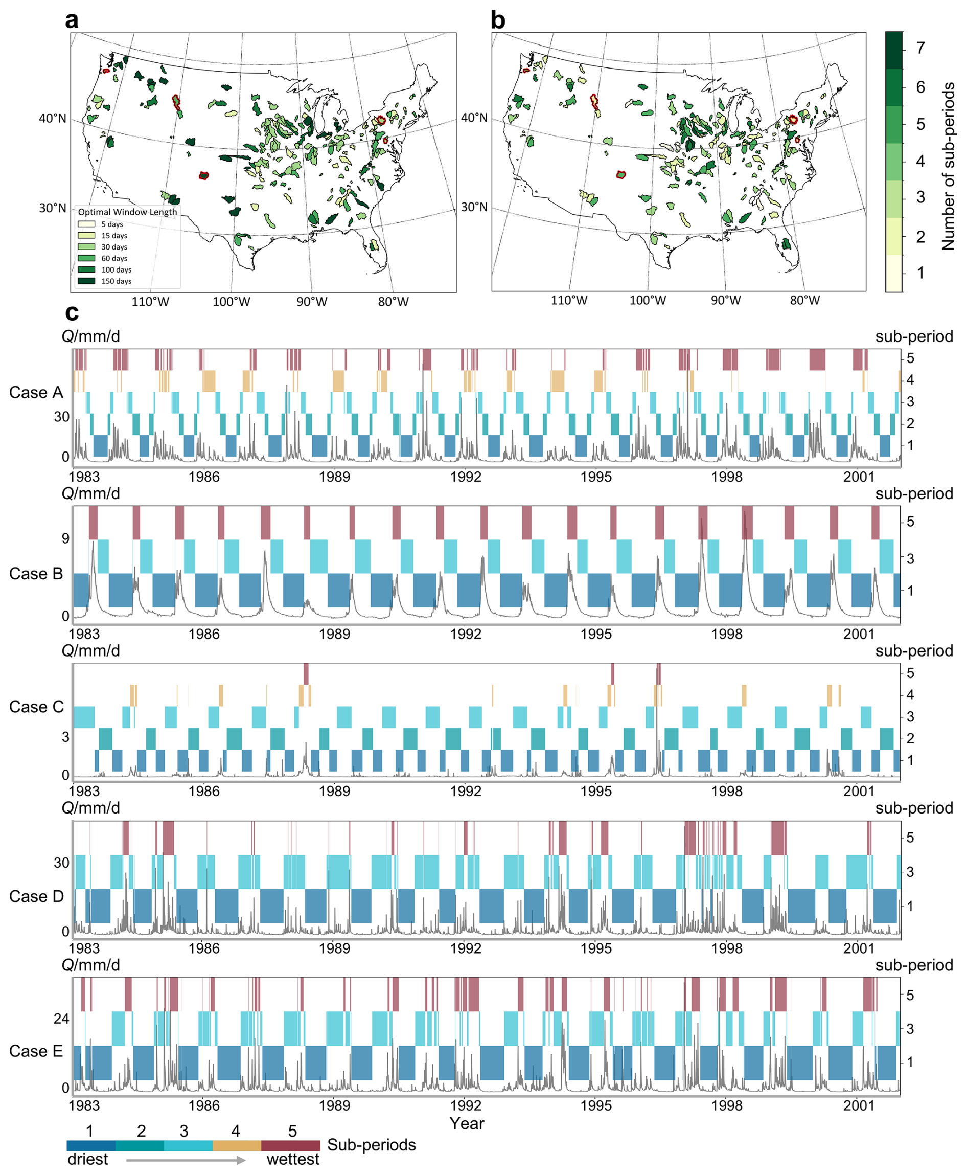
Figure 3 (a) Optimal window lengths of the catchments used in this study for the sub-period clustering. (b) Number of sub-periods reflecting results from Sect. 3.2. (c) Visualization of clustering results on the hydrograph for the study cases, where colors indicate reordered sub-periods ranked from driest to wettest according to mean streamflow, with a consistent color mapping across the entire time series.

Analysis of the statistical properties of each sub-period (Sect. S2.3) indicates that the identified sub-periods are closely associated with underlying physical and climatic drivers. Across the representative cases, the sub-periods consistently correspond to distinct hydrological states shaped by variations in evaporative demand, antecedent storage, runoff response, and the relative contributions of quick flow and baseflow, rather than arbitrary temporal clustering. These physically interpretable sub-periods provide a robust basis for subsequent dynamic parameterization and modelling experiments. In addition, two diagnostic comparative analyses are presented in Sect. S5 to further evaluate whether the observed performance improvements arise from improved representation of catchment dynamics rather than increased parameter dimensionality. Considering the performance of the seven modelling experiments across both calibration and evaluation periods, Experiments 5 and 7 are considered the recommended experiments for capturing dynamic catchment characteristics (Fig. 4). Experiment 5, with multi-parameter dynamic calibration, achieves high predictive accuracy across diverse flow regimes, although it may slightly compromise physical consistency in runoff generation. Experiment 7, incorporating smooth parameter transitions, maintains comparable accuracy while promoting more consistent and physically reasonable runoff strategies across sub-periods, thus offering a balanced approach between model performance and hydrological interpretability. Detailed analysis of the results will be presented in the following sections.

4.2 Model performance

To compare seven experiments in dynamic catchments and to identify potential limitations in model calibration, the evaluation is conducted across 219 catchments characterized by hydrological variability. As shown in Fig. 4, the NSE and LNSE values during both calibration and evaluation periods reveal differences in the ability of diverse calibration schemes to capture high- and low-flow conditions. The median NSE reached only 0.4–0.5 in Experiments 1 and 2, and although the LNSE approached 0.7, negative values are frequently observed. It is suggested that global optimization or simple weighted objective functions often lead to an averaging of catchment responses, thereby limiting accuracy for both high- and low-flow conditions. Experiment 3 employed an objective function defined as: OF = 0.27 ⋅ RMSE_Q5 + 0.16 ⋅ RMSE_Q20 + 0.08 ⋅ RMSE_Qmid + 0.24 ⋅ RMSE_Q70 + 0.25 ⋅ RMSE_Q95, the weighting scheme explicitly accounted for extremely high (Q₉₅), high (Q₇₀), medium (Q_mid), low (Q₂₀), and extremely low (Q₅) flows. Despite this design, both NSE and LNSE declined relative to Experiment 1. The decrease may be attributed to excessive parameter adjustments aimed at fitting a limited number of extreme events, which reduced the predictive accuracy of the overall streamflow process. When single dynamic parameters are introduced in Experiment 4, median NSE and LNSE increased to approximately 0.55 and 0.8, respectively, with narrower interquartile ranges. These outcomes indicate that dynamic parameters enhanced the ability of the hydrological model to capture temporal variability, although structural errors persisted, as reflected in local outliers. Experiment 5 achieved median NSE and LNSE values of approximately 0.7–0.8 in both calibration and evaluation periods. Although high-dimensional optimization increased computational demand and LNSE variability in some basins, overall performance represented a balanced trade-off between dynamic adaptability and physical consistency. Experiment 6 also performed well during the calibration period; however, its abrupt parameter switching led to a decline of LNSE and increased dispersion in the evaluation period. Experiment 7 addressed these shortcomings by applying a gradual parameter-switching strategy during the evaluation period. As shown in Fig. 4, the boxplots are more compact and shifted toward higher values, indicating that stable and consistent performance was achieved across most basins. However, compared with Experiment 5, Experiment 7 displayed a greater number of outliers, particularly in LNSE, where they tended to cluster at lower values, suggesting higher variability in model performance across catchments. The overall accuracy remained comparable to that of Experiment 5. In summary, compared with static calibration schemes (Experiments 1–3), single dynamic parameter calibration (Experiment 4) improved simulation accuracy, while multi-dynamic parameter calibration produced further gains. Among all experiments, Experiments 5 and 7 demonstrated the most robust and accurate performance. Representative catchments further confirm the basin-scale conclusions. Across all five cases, Experiments 5 and 7 consistently maintain superior performance during evaluation, with improved robustness across flow phases. Detailed multi-metric results for the five representative cases are provided in Sect. S3.

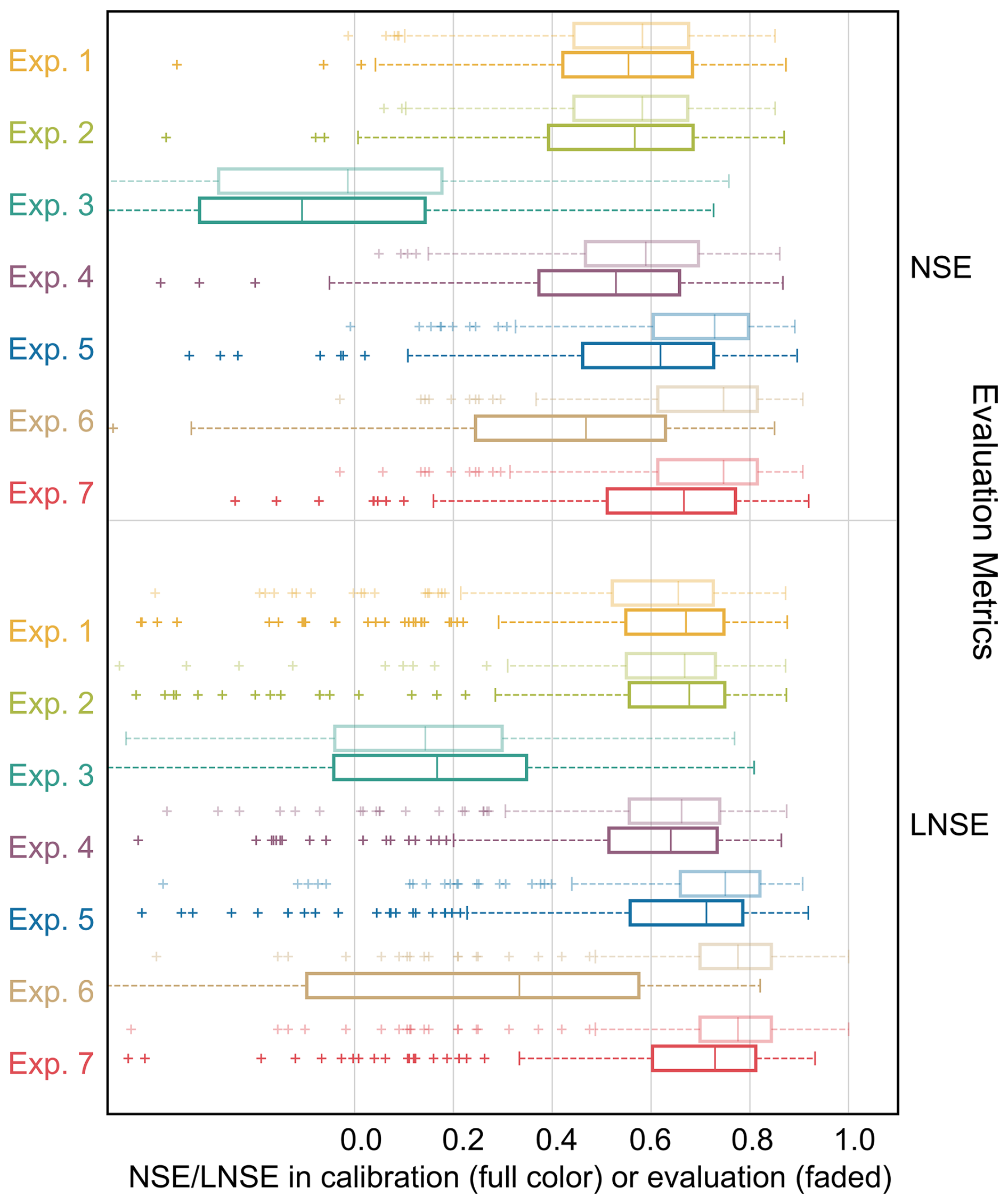
Figure 4 Performance of seven calibration experiments on the MOPEX dataset across 219 catchments. Boxplot colour denotes different experiments. The whiskers extend a maximum of 1.5 times the interquartile range. Values beyond the whiskers are marked as outliers and are denoted as +.

4.3 State variables and fluxes

The state variables and fluxes reflect the internal operation of the hydrological model. The assessment results of state variables and fluxes through seven calibration experiments for case A are illustrated in Fig. 5 (results of cases B, C, D, and E are shown in Sect. S6). Experiments 1, 2, and 3 exhibited only minimal differences in both state variables and flux time series, with only the results of Experiments 1 and 3 shown for clarity. A slight improvement is shown in Experiment 4 compared with the time-invariant parameter schemes; however, small mismatches remain during flow recessions and peak timings. This indicates that the dynamic adjustment of a single parameter is insufficient to represent the full range of catchment dynamics. In Experiment 6, abrupt parameter switching is applied across sub-periods. The state variable X_q and flux Q_q in Experiment 6, exhibit step changes or even discontinuities at the switching boundaries, with large deviations during low-flow sub-periods. The phenomenon is particularly evident in cases B and D. These results indicate that abrupt switching disrupts water balance continuity, thereby reducing performance in low-flow simulations. Despite these setbacks, Experiments 5 and 7 introduced significant improvements across all study cases. In Experiment 5, multi-parameter dynamic calibration is applied while continuity of state variables and fluxes is maintained. As shown in Fig. 5, in case A, the flux variables Q_q andQ_S transition smoothly across sub-periods without visible discontinuities, the state variables XH_uz and XC_uz also connect consistently across sub-periods, indicating that multi-parameter dynamic calibration captures the catchment dynamics of soil moisture and storage processes. However, Experiment 5 shows limitations in maintaining the consistency of simulated discharge (Q_sim). For example, in case B, the baseline extent of Q_sim exhibited slight drift, reflected in systematic differences in response intensity to similar rainfall events across adjacent sub-periods. The fluxes and state variables in Experiment 7 exhibit results similar to those in Experiment 5. However, when sub-period simulations are concatenated, slight inconsistencies occasionally emerge at the sub-period boundaries, with flood peaks being slightly overestimated or baseflows being underestimated. A comparative flux-mapping analysis of Experiments 1, 5, and 7 is provided in Sect. S6 to further examine differences in runoff component consistency and parameter equifinality across sub-periods.

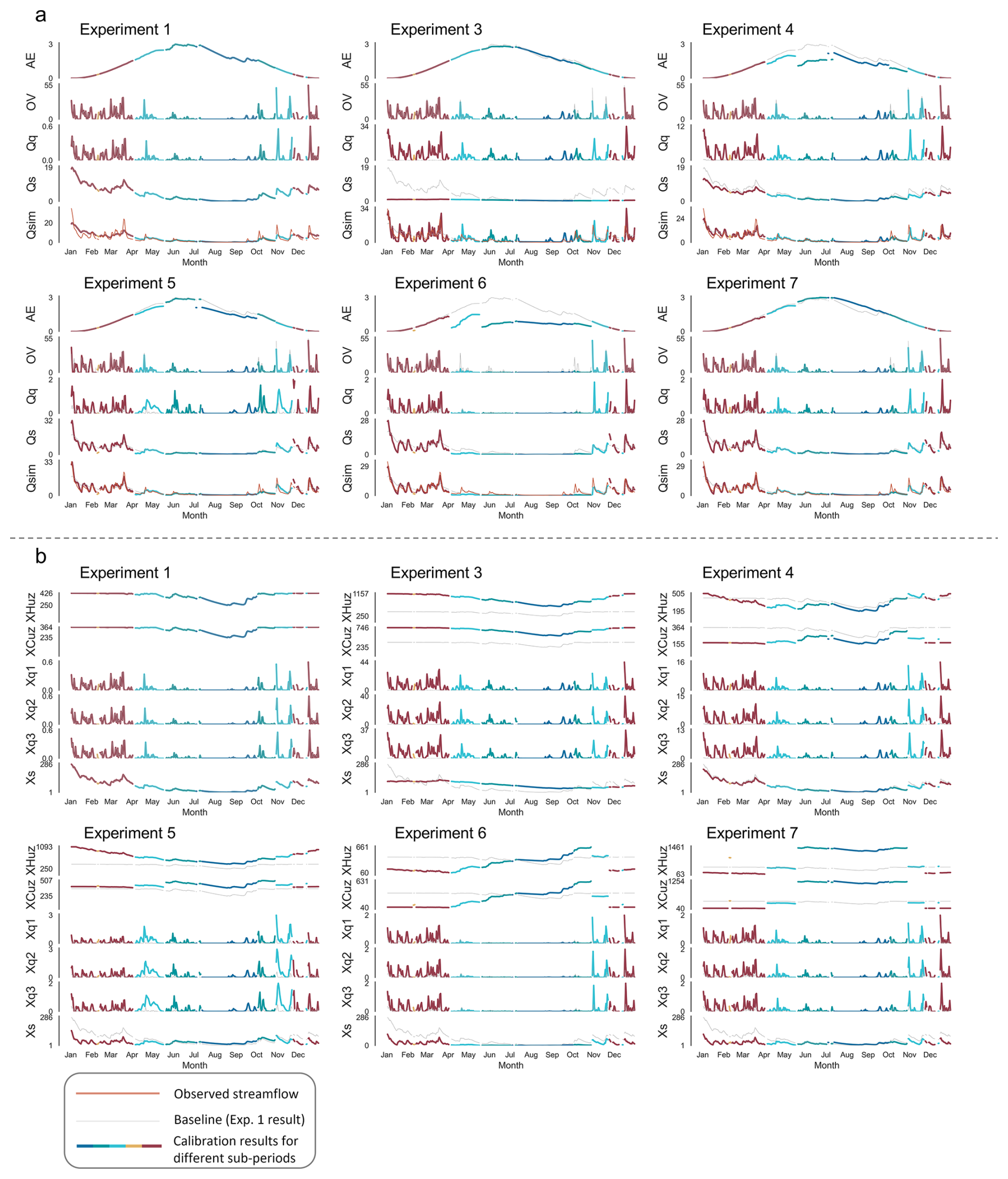
Figure 5 Simulation results of (a) fluxes and (b) state variables for Experiments 1–7 in Case A during 1998, a representative year from the middle of the evaluation period. Different colours denote different identified sub-periods.

5 Discussion

5.1 Why dynamic parameter sets improve simulation performance

Despite the significant improvement in the simulation performance of hydrological models based on catchment dynamics, analyses of dynamic parameter behaviour (presented in Sect. S7) indicate that the response of discretized dynamic parameters (even highly sensitive ones) to these catchment dynamics is not satisfactory. However, a dynamic parameter set can collectively carry the extracted information of dynamic catchment characteristics, compensating for model structural deficiencies and improving model performance. Therefore, this study further explores the potential reasons from three aspects: the correlations between parameters, equifinality in the hydrological model, and the evolution process of parameters.

5.1.1 Complex correlation between parameters

Figure 6a and c demonstrate that there are both significant linear and nonlinear correlations among the parameters of the hydrological model in case A (results of other cases are shown in Sect. S8). MIC values above 0.35 among most parameters suggest that the dynamics of individual parameters may be affected by others (Gillespie et al., 2021). This explains the unimproved model performance when altering individual parameters during different sub-periods in Experiment 4. The analysis results of parameter sensitivity based on the scatter plot method also confirmed the influence of the correlation between parameters. In the recommended scheme (Experiment 7), parameters like K_s (the slow-flow routing tank's rate) exhibit a weak responsive relationship to the dynamic catchment, validating the significance of clustering sub-periods based on catchment dynamics. Due to the complex linear or nonlinear correlations between parameters, the variation of individual parameters can be compensated for by changes or adjustments in other parameters, leading to no significant changes in the simulation performance of the model (Xiong et al., 2019; Gou et al., 2020; Zhou et al., 2022). Bárdossy (2007) suggested that parameters within a hydrological model parameter group should not be considered individually but rather treated as a whole.

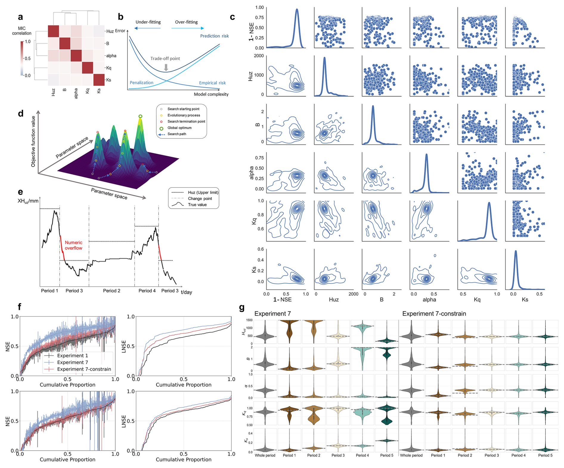
Figure 6 (a) Linear or nonlinear correlations between parameters based on MICs in case A, with red indicating the strongest correlation among parameters. (b) Conceptual diagram illustrating the trade-off between empirical fitting to data and the penalization of model complexity, and its impact on prediction error (Schoups et al., 2008). (c) Parameter sensitivity analysis for case A through scatter plots. (d) Three-dimensional fitness landscape showing the objective function values on the vertical axis, parameter space on the horizontal axis, and various evolutionary paths that elements can follow within the parameter space, indicated by arrows. (e) Conceptual diagram of errors resulting from abrupt parameter shifts. (f) Cumulative distribution functions (CDFs) of NSE and LNSE comparing the experiment built on Experiment 7 with added parameter constraints (blue), Experiment 7 (red), and Experiment 1 (black); higher values indicate better performance. Upper panels show calibration; lower panels show verification. Shaded bands denote 90 % bootstrap confidence limits to indicate sampling uncertainty. (g) Distributions of the optimal parameter spaces across sub-periods under different climatic and land-surface conditions for case A. Each violin depicts one parameter space, with parameter values on the y-axis; the violin width reflects the probability density of the parameter values. Parameter bounds are: H_uz (0–1500), B (0–2), α (0–1), K_q (0.5–1), and K_s (0–0.5). Results for all study cases are provided in Sect. S9.

5.1.2 Equifinality in the hydrological model

The parameter sets derived by the SCE-UA algorithm for flux mapping encounter inherent limitations (Beven, 1993; Padiyedath Gopalan et al., 2018). This arises due to the algorithm's inherent directionality in the optimization process, which potentially overlooks certain parameter sets capable of producing equifinality results. Analysis of parameter sensitivity through flux mapping and scatterplot methodology reveals a distinctive feature towards the end of the search path: A tail-like pattern in the scatterplot in Fig. 6a and b, indicating a series of parameter sets with equifinality identified by the optimization algorithm. These scatter points represent parameter sets producing similar results, though originating from distinctly different physical processes. Hence, it may fail to infer that model runs exhibiting higher performance values consistently correspond to more realistic scenarios. The evaluation of model performance, particularly when quantified in a scalar manner, emerges as a weak, unreliable, and unrealistic approach for model assessment. The representation of model processes cannot be sufficiently measured by a solitary performance metric or a limited range of values (Khatami et al., 2019; Knoben et al., 2020). A rigid interpretation of objective functions can lead to misinterpretations; for instance, in Fig. 6b, model runs with marginally lower NSE values might offer more realistic underlying processes compared to those with better NSE values (Gomez, 2019). It is vital to acknowledge that high model performance does not inherently equal realism and may be influenced by numerical artifacts arising from various sources of uncertainty. Moreover, our constrained understanding of catchment processes, involving runoff generation mechanisms and complex runoff events, makes it challenging to determine the likelihood of specific parameter sets occurring in reality (Troin et al., 2021).

5.1.3 Evolution process of parameters

While the causes of non-physical dynamic parameter values are complex, they might be partially attributed to the failure of global optimization algorithms to converge and find approximate global optimal solutions during the evolutionary process. Hydrological model parameter response surfaces exhibit a range of complex characteristics, including high non-linearity, multi-modality, non-convexity, irregularity, discontinuity, noise, roughness, and non-differentiability (Bian et al., 2024; Herrera et al., 2021). To better describe the evolutionary process of the parameters, a fitness landscape is used, where the vertical axis represents the objective function values and the horizontal axis represents the parameter space (Fig. 6d). The evolutionary process is the process of searching for a global optimum. During this process, deceptive gradients of the objective function values can mislead the optimizer away from the global optimum; the increase in the number of local optima also makes the search path for the global optimum more complex and challenging (Bian et al., 2024). Terminating at a local optimum can prevent the optimized parameters from accurately responding to environmental changes.

5.2 Problems caused by parameter abrupt shifts

Abrupt parameter shifts disrupt the assumption of long-term water balance in traditional hydrological models, potentially leading to invalid values for state variables in adjacent sub-periods (Myers et al., 2021; Lakshmi and Sudheer, 2021). For instance, during the transition of soil maximum storage height (H_uz), the H_uz value for the next sub-period might be lower than the former actual state variable value (XH_uz). Similarly, numerical overflow errors might lead to model crashes and the generation of invalid results (Fig. 6e). These errors could also propagate through various modules of the model, such as the high-speed runoff module and slow-speed runoff module, disrupting the proper functioning of other parts of the model and making the optimization algorithm incapable of producing valid results.

5.3 Parameter response to catchment dynamics

In this study, the sub-period clustering method (Sect. 3.2) is used to extract temporally varying catchment information, allowing model parameters to adjust across distinct hydrological periods. The resulting improvements in simulation accuracy and robustness highlight the value of incorporating time-varying parameters into hydrological models (Refsgaard et al., 2021). A key question, however, is whether these parameter variations reflect genuine changes in catchment behaviour or primarily compensate for structural limitations of the model itself (Thornton et al., 2022). To address this problem, a diagnostic experiment is designed. Building on the sub-period calibration framework (Experiment 7), a soft constraint based on globally optimal parameters is introduced, integrating prior information on overall catchment behaviour into sub-period parameter estimation. This design balances the flexibility of dynamic parameter adjustment with the need to preserve physical consistency. The diagnostic objective function is defined as:

$$\begin{array}{}\text{(2)}& \mathrm{OF}=\mathrm{1}-(\mathrm{0.5}\times \mathrm{NSE}+\mathrm{0.5}\times \mathrm{LNSE})+\mathrm{Penalty}\end{array}$$

where the penalty term quantifies the deviation of the sub-period parameter set ${\widehat{\mathit{\theta }}}_i$ from the globally optimal parameter set θ_i. The penalty is formulated as the mean of the absolute relative errors: Penalty $=\frac{\mathrm{1}}{N}\times \sum \left|\frac{{\widehat{\mathit{\theta }}}_i-{\mathit{\theta }}_i}{{\mathit{\theta }}_i}\right|$, where i denotes the parameter index, and N is the total number of parameters (HYMOD). This setting allows assessment of how model responses change when parameter variability is constrained within a more stable and physically consistent range.

As shown in Fig. 6f and g, the imposed constraint produces more concentrated posterior parameter distributions and improves parameter transferability between calibration and evaluation periods. However, these gains are accompanied by clear reductions in NSE and LNSE relative to unconstrained dynamic calibration, indicating that part of the performance improvement under dynamic calibration arises from compensation for structural deficiencies in the fixed model formulation. The results suggest that the need for dynamic parameters is closely linked to the incomplete representation of key hydrological processes. Within this context, the proposed dynamic calibration framework provides a practical strategy for using dynamic parameters as proxy variables to partially account for unresolved structural limitations and improve streamflow simulation in dynamic catchments (Beven, 2019).

6 Conclusions

Due to limitations in observational data and an incomplete understanding of catchment hydrological processes, traditional conceptual hydrological models often fail to represent dynamic catchment characteristics, leading to generalized simulation of different flow regimes. To address model deficiencies and improve simulation in dynamic catchment characteristics, it is essential to re-examine the time-varying information in historical hydrological and meteorological data and consider the variation in calibration. The study investigates calibration challenges in dynamic catchments and proposes a structured framework to address two major issues: the influence of objective function design on flow-phase-specific performance and the limitations of sub-period calibration with dynamic parameters. Seven experiments were conducted to systematically evaluate these aspects. Experiments 1–3 focused on the effects of time-invariant parameters and different objective function configurations, while Experiments 4–7 explored challenges in dynamic parameter calibration, including parameter correlation, high dimensionality, and state transitions. Model performance was comprehensively assessed using multiple metrics and internal diagnostics across 219 MOPEX catchments. The following specific conclusions could be drawn from this study:

• Adjusting the configuration of the objective function can enhance the simulation of emphasized flow phases, but at the cost of sacrificing simulation performance for other flow phases, making it difficult to improve overall model performance.

• Due to issues of model structural deficiencies, correlation among parameters, high dimensionality in optimization, and the transition of dynamic parameters between adjacent sub-periods, improving model performance through individual parameters alone is not feasible. Model parameters should be considered as a group of parameters.

• Among all calibration experiments, Experiments 5 and 7 effectively addressed the challenges associated with dynamic parameter operations and flow-phase-specific performance, balancing dynamic adaptability and physical consistency. These calibration strategies are thus recommended for application in dynamic catchments, where capturing temporal variability and maintaining model reliability are critical.

The calibration and evaluation framework proposed in this study not only addresses defects caused by the simplification of model structure for hydrological models but also enhances model simulation accuracy across different flow phases and effectively reduces model uncertainty. The evaluation framework comprehensively assesses the performance of hydrological models through multi-criteria evaluation and reveals sources of uncertainty in model internal operation from the perspectives of state variables and fluxes. Despite the positive results of this study, developing more realistic models will aid in our understanding of hydrological processes and improve hydrological forecasting.