Community-scale urban flood monitoring through fusion of time-lapse imagery, terrestrial lidar, and remote sensing data

High-frequency flood events in urban areas pose significant cumulative hazards. These floods are often difficult to detect and monitor using existing infrastructure, making the development of alternative approaches critical. This study presents the implementation of a computer vision-based urban flood monitoring network deployed in Cahokia Heights, Illinois, USA. Flood observations were collected at 30 min intervals using consumer-grade trail cameras. Water surface elevations were estimated from the intersection of segmented flood masks with 2D-projected terrestrial lidar data. Flood extents and depths were extrapolated using a terrain depression-filling algorithm. Camera-derived peak flood extents and depths were compared to independent predictions from a 2D HEC-RAS Rain-on-Grid flood model. This procedure was applied to two flood events, one moderate and one severe, using imagery from two camera sites. For the severe event, water level estimates agreed closely between cameras, with a median difference of less than 3 cm and a peak difference of less than 2 cm. For the moderate event, differences were larger (median<10 cm, peak<16 cm). Agreement between modelled and camera-derived peak flood extents exceeded 90 % for the severe event but ranged between 21 % and 42 % for the moderate event. We use the convergence and divergence of independent camera observations to infer differences in spatiotemporal flood connectivity, disconnected in the moderate event and connected in the severe one. This study demonstrates the utility of low-cost, camera-based systems for high-resolution monitoring of flood dynamics in complex urban environments and highlights their potential integration with hydrodynamic modelling.

1 Introduction

Flooding is the single most economically destructive natural hazard within the United States. Between 1960 and 2016, an estimated 73 % (USD 107.8 billion) of direct flood property damage in the United States occurred in urban areas (National Academies of Sciences Engineering and Medicine, 2019). The risk and impacts of urban flooding are projected to increase in coming decades, driven by climate change, expanding urban populations, and land-use change (O'Donnell and Thorne, 2020). For many regions, climate models project an increased frequency of short duration, high-intensity rainfall events, increasing flood risk in urban areas (Fowler et al., 2021a, b). At the same time, the rate of urbanization in high flood-risk areas has outpaced other areas since 1985, increasing flood exposure risk of the general population (Rentschler et al., 2023). Together, climate and population changes are projected to lead to an increase of 300 million people exposed to a 1 % annual risk of flooding (Rogers et al., 2025).

Both current assessments and future projections of urban flood risk frequently find significant socioeconomic disparities related to flood risk exposure both at national and local scales (Fan et al., 2025). At the national level, lower income nations are experiencing more rapid floodplain urbanization (Mazzoleni et al., 2020). For individual cites, vulnerable communities – including low-income communities and communities of color – are both exposed to more frequent flooding and experience disparate impacts (Ma and Mostafavi, 2024; Selsor et al., 2023; Qiang, 2019). Neighborhood-scale differences in flood exposure, which can be driven by local differences in impervious area, microtopography, and stormwater infrastructure, are often not resolvable in metropolitan or regional-scale flood assessments (Helmrich et al., 2021; Schubert et al., 2024). Mitigating these small-scale spatial differences in flood hazards requires equivalently high-resolution monitoring of flood frequency and intensity. Most often, this type of localized risk assessment cannot be accomplished without substantive cooperation and collaboration with impacted communities (Azizi et al., 2022).

Pluvial flooding, which occurs when precipitation intensity exceeds local drainage capacity, can significantly impact urban environments, perhaps making it surprising that it has received comparatively less attention from researchers and policymakers (Rosenzweig et al., 2018; Prokić et al., 2019). Unlike fluvial flooding, which is typically linked to overflowing rivers and streams, pluvial flooding is driven by local surface water accumulation, particularly during short-duration, high-intensity rainfall events (Rosenzweig et al., 2018; Azizi et al., 2022). Pluvial flooding is particularly relevant in urban landscapes, where low-lying topography and high impervious surface coverage promote rapid runoff generation (Agonafir et al., 2023). In its early stages, pluvial flooding is often characterized by spatially isolated patches of water collecting in local topographic depressions (Rosenzweig et al., 2018; Mediero et al., 2022; Cea et al., 2025). As rainfall continues, these patches may overflow and merge, creating dynamic and expanding flood networks (Samela et al., 2020). Urban topography and infrastructure, such as roads, buildings, and stormwater systems, exert strong control on these patterns, simultaneously directing, constraining, or amplifying surface flow (Balaian et al., 2024; Beteille et al., 2025; Fan et al., 2020). Engineered drainage, such as stormwater systems, can far exceed soil infiltration in urbanized watersheds (Agonafir et al., 2023). Depending on their capacity, and condition, stormwater infrastructure can both alleviate flooding when functional but also contribute to surface runoff when drainage capacity is exceeded (Tran et al., 2024).

Despite its frequency and growing relevance, pluvial flooding is often excluded from traditional flood risk assessments (Rosenzweig et al., 2018; Prokić et al., 2019). Whereas fluvial flooding tends to drive large, low-recurrence events, pluvial flooding is associated with higher-frequency, lower-magnitude events – often termed “nuisance floods” because they do not typically pose an immediate threat to public safety (Rosenzweig et al., 2018; Moftakhari et al., 2018). However, their cumulative socio-economic impact over time can rival that of rare, extreme flood events, especially when the broader impacts of flood damage include transportation disruption, public health risks, and wastewater ingress into buildings (Moftakhari et al., 2017; Ten Veldhuis, 2011; Ten Veldhuis et al., 2010). In the Netherlands, the 10 year cumulative impact of smaller pluvial floods was estimated to nearly equal to the damage of a single 125 year recurrence flood event (Ten Veldhuis, 2011). In the United States, damage from pluvial floods is typically excluded from the National Flood Insurance Program, making it difficult to estimate their total economic impact (Azizi et al., 2022; National Academies of Sciences Engineering and Medicine, 2019). However, a recent study found that 87 % of flood insurance claims for properties outside the FEMA-defined 100 year floodplain between 1978 and 2021 were likely related to pluvial flooding, with over 68 % linked to events with less than a one-year recurrence interval (Nelson-Mercer et al., 2025). Similar findings in the United Kingdom found that 83 % of reported flood damages occurred outside of designated floodplains or coastal areas, indicative of local pluvial flooding. Further, these reported damages were likely to affect properties repeatedly, highlighting the cumulative impacts of high frequency events (Dawson et al., 2008). Although data gaps remain, these recent studies provide strong evidence that pluvial flooding poses a widespread and frequently underestimated risk, motivating more comprehensive monitoring and inclusion of pluvial floods in flood risk assessments (Rosenzweig et al., 2018; National Academies of Sciences Engineering and Medicine, 2019).

Monitoring and predicting pluvial nuisance floods present distinct challenges. Existing fluvial monitoring infrastructure, such as stream gages and water surface sensors, is not suited to detect disparate flood patches disconnected from the monitoring river system or stream (Song et al., 2024; Griesbaum et al., 2017). Flood extents extrapolated from water surface levels recorded by these sensors tend to underestimate pluvially-driven flood extents, which can occur even when stream levels are below flood stage (Cea et al., 2025). To overcome these limitations, researchers have increasingly turned to distributed sensor networks to better capture the spatial heterogeneity of urban flooding (Lo et al., 2015; Song et al., 2024; Zhong et al., 2024; Mydlarz et al., 2024; Mousa et al., 2016; Azizi et al., 2022). Both contact sensors (e.g., pressure transducers) and non-contact sensors (e.g., radar, ultrasonic), have proven effective for monitoring distributed urban flooding (Mydlarz et al., 2024; Gold et al., 2023). However, they can face operational challenges for small-scale flooding in urban settings, including limited installation locations and sensitivity to local disturbances (Song et al., 2024). For example, the radar based FloodNet system was limited at many sites to placement over sidewalks, limiting observation of early road flooding (Mydlarz et al., 2024). Further, water level sensors of this nature, even when spatially distributed, only record point measurements of water level, which require further interpolation to create spatially extensive flood maps. Satellite-based and UAV remote sensing offer broader spatial coverage and, thus, have become widely used tools for flood extent mapping across a range of environments and scales (Allen and Pavelsky 2018; Tellman et al., 2021; Chanda and Hossain, 2024). However, these methods are constrained both by coarse (>1 m) spatial and temporal (>1 d return time) resolution, making them less effective for short-duration floods and small-scale urban nuisance flood events (Tarpanelli et al., 2022; Tulbure et al., 2022; Chanda and Hossain, 2024; Zhu et al., 2022; Composto et al., 2025).

In contrast, ground-based cameras offer a promising and scalable alternative, addressing the challenges of both in-situ sensors and remote-sensing approaches (Lo et al., 2015). Ground-collected imagery provides spatially coherent measurements of flood extent within the camera's field of view, capturing continuous water surfaces in each frame, rather than isolated point readings. When deployed using consumer-grade equipment or existing infrastructure, such as traffic or security systems, cameras provide a low-cost way to achieve broad spatial coverage across urban areas (Wang et al., 2024; Lo et al., 2015). Cameras deliver high temporal resolution imagery through frequent image capture, enabling detailed tracking of flood dynamics over time. This near-continuous visual monitoring facilitates rapid flood detection and analysis, especially when combined with automated image processing techniques. Ground-collected images also capture rich contextual information, including visible landmarks, infrastructure, and human activity, enhancing the interpretation of flood impacts and supporting more comprehensive urban flood management.

There are three broad approaches to camera-based flood monitoring. The first and most developed relies on identifying water levels relative to known benchmarks, such as topographic markers or staff gauges. This approach is particularly well-suited to river or reservoir environments, where stage progression and flooding is more predictable (Sabbatini et al., 2021; Chapman et al., 2022, 2024; Johnson et al., 2025). However, its applicability can be limited when flood extents are irregular or spread over complex urban terrain without extensive available benchmarks from which water levels can be derived. A second approach uses the fraction of an image classified as flooded to estimate water level and extent. This method requires the development of a quantitative correlation between flooded image fraction and water level (de Vitry et al., 2019; Vandaele et al., 2021). Hybrid methods combine both techniques, using image segmentation and reference objects to estimate flood depths. For example, Vandaele et al. (2021) used surveyed landmarks to constrain absolute water level. Liang et al. (2023) used the automated identification of street signs and humans in flood images to estimate water depth. While shown to be promising, these methods often depend on stable camera positions, consistent lighting, and persistent ground control points.

A key limitation of image-only flood monitoring approaches is their difficulty in translating two-dimensional image pixel data into real-world flood depths, particularly in heterogeneous urban landscapes where water may accumulate in shallow, discontinuous patches. More advanced methods have addressed this challenge by integrating camera imagery with high-resolution topographic data, such as lidar or Structure-from-Motion (SfM) (Wang et al., 2024; Griesbaum et al., 2017). Pairing high-resolution topographic data products with known camera geometries allows floodwater-identified pixels to be geo-referenced and intersected with the underlying terrain, yielding spatially distributed flood depths even in settings where flood boundaries are irregular or flood waters evolve rapidly (Erfani et al., 2023; Eltner et al., 2018, 2021). As a result, these methods can overcome the spatial ambiguities inherent in image-based approaches and are particularly valuable in the complex topography of urban environments. However, most demonstrations of this technique have occurred in controlled or short-term deployments with stable cameras and ground control, with the notable exception of Blanch et al. (2026), which successfully applied projection-based stream level estimation over a continuous two-year period. The feasibility of its use for long-term flood monitoring in urban environments, with limited ground control, and frequently changing scene context, requires additional research.

Camera-based flood monitoring approaches ultimately rely on robust image segmentation to accurately identify water presence and extent. Traditional image processing techniques such as intensity thresholding and random-forest classification remain useful in structured environments (Chapman et al., 2024; Lo et al., 2015; Griesbaum et al., 2017), but most recent work has transitioned towards deep learning-based semantic segmentation models to classify water pixels (Erfani et al., 2023; Eltner et al., 2021; Wang et al., 2024). Architectures range from U-Net models (Vitry et al., 2019), to more complex vision transformers (Erfani et al., 2023; Zamboni et al., 2025), with many models achieving high segmentation accuracy when trained on domain-specific datasets. Indeed, a systematic evaluation of 32 network architectures trained on the same dataset of river images demonstrated the efficacy of the method, with 24 of the tested architectures achieving greater than 90 % testing accuracy (Wagner et al., 2023). The recent emergence of foundation models such as Segment Anything (SAM) (Kirillov et al., 2023; Ravi et al., 2024) has introduced the possibility of domain-agnostic water segmentation. Recent studies have demonstrated that with minimal fine tuning, these domain-agnostic foundation models can achieve comparable classification accuracy to state-of-the-art, domain-specific models (Moghimi et al., 2024; Wang et al., 2024).

In this study, we present a flexible and operationally oriented framework for monitoring urban flood extent and depth using time-lapse imagery from ground-based cameras in combination with terrestrial and aerial lidar data. Our implementation focuses on a community in Cahokia Heights, IL experiencing chronic pluvial flooding within the Mississippi River floodplain. Using consumer grade trail-cameras, we demonstrate accurate, centimeter-scale, water level estimation, and flood extent extrapolation, for two case study flood events. Our approach emphasizes adaptability to site conditions, minimal reliance on fixed benchmarks, and limited need for long-term infrastructure. We additionally compare our camera-derived estimates with output from a two dimensional, HEC-RAS rain-on-grid hydrodynamic model, as a proof of concept for integrating camera-based monitoring in operational flood modeling workflows.

2 Methods

2.1 Study site

Flood monitoring efforts were conducted in collaboration with the Cahokia Heights community, located in St. Clair County, Illinois, within the Mississippi River Floodplain (Fig. 1a). Cahokia Heights residents have long experienced chronic nuisance flooding, driven primarily by pluvial processes (U.S. EPA, 2021; Maganti, 2020; Colten, 1988; Schicht, 1965). Despite the occurrence of multiple impactful floods each year, the entirety of area presented in this study falls outside of FEMA defined Special Flood Hazard Areas (FEMA, 2003). This frequent flooding is attributable to both natural and engineered factors. The region's clay-rich floodplain soils exhibit poor drainage, and in combination with the low-relief landscape (Fig. 1b–d), water readily accumulates in surface depressions (USACE, 2023). Compounding these natural vulnerabilities, decades of infrastructure neglect have left the sewer and stormwater systems in disrepair. Many of the existing sewer and stormwater pipes are undersized or blocked, reducing drainage capacity and leading to recurrent sewage backups and drinking water contamination (USACE, 2024a). As a result, persistent flooding has caused significant property damage, disrupted the daily activities of residents, and compromised household plumbing systems (Musiker et al., 2021). At the time of this study, no formal flood monitoring infrastructure existed within the community.

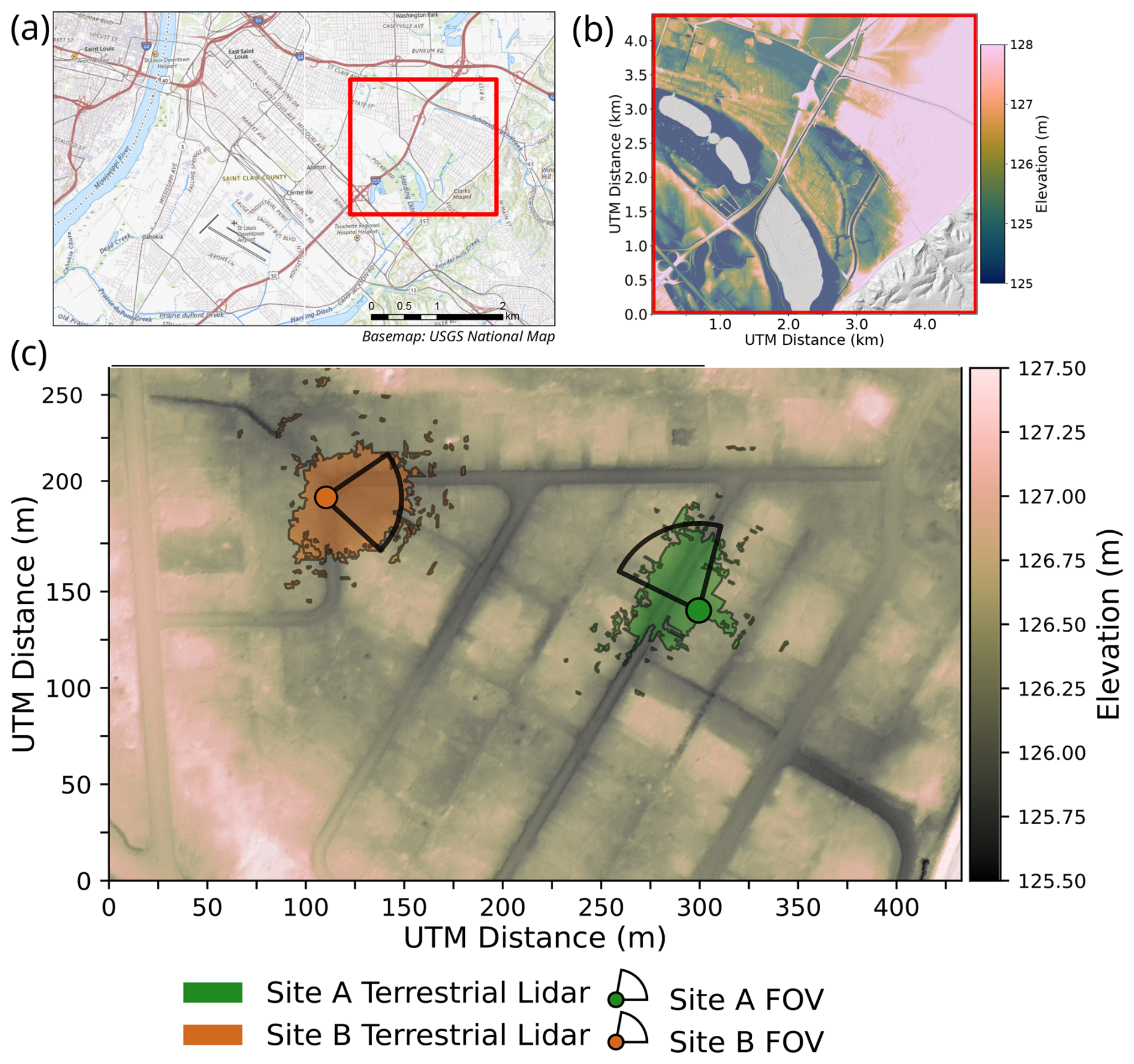
Figure 1 (a) Study location of Cahokia Heights, IL (b) broader study area shaded relief (c) Terrestrial lidar point cloud extent and camera monitoring location field of view (FOV). Color ramps in panels b and c are batlow and turku, respectively (Crameri, 2023).

2.2 Community-scale monitoring network

To begin addressing this gap, eight time-lapse camera flood monitoring stations were installed in the fall of 2020 in collaboration with community residents. This study focuses on two of those stations, herein Sites A and B (Fig. 1b). Cameras A and B are located on opposite sides of a residential neighborhood, approximately 190 m apart, with non-overlapping fields of view. Camera A is positioned on a straight stretch of road on the eastern side of the neighborhood at an elevation of 126.1 m (NAVD88). Camera B is located on the western side of the neighborhood, at a slightly lower elevation of 125.95 m, placed at a slight bend in the road (Fig. 1c). Each monitoring station consists of a Blaze A52 trail-camera (16 MP, f4 mm) in a transparent-faced plastic housing mounted approximately 1.5 m off the ground on metal conduit pipe driven into the soil. Each camera is set to capture a 5120 by 2880-pixel resolution image and a five second video every 30 min. Due to excessive glare during nighttime operations, the cameras' infrared flash was disabled, and ambient lighting from streetlights was used for nighttime operation. Images were retrieved approximately every two months during site visits, during which batteries and SD cards were replaced. Camera disturbances, motion, or damage were documented at each service interval.

This study draws on two primary sources of topographic data: a regional aerial lidar survey and terrestrial lidar acquired at each camera site in 2023. The aerial lidar dataset was collected across St. Clair County in 2019 as part of the USGS 3D Elevation Program (3DEP) and the Illinois Height Modernization Program (ILHMP) (Aerial Services Inc, 2021; USGS, 2022). LAS-format point clouds were obtained for the study area, with an average point density of 4.0 points m⁻². These data were interpolated into a 0.5 m resolution digital terrain model (DTM) using inverse distance weighting (IDW), implemented via the Point Data Abstraction Library (PDAL) (Butler et al., 2024). Additionally, a void-filled DTM at the same resolution was created using triangulated irregular network (TIN) interpolation. This processed product is referred to throughout the paper as the USGS DTM.

While aerial lidar offers broad spatial coverage, it does not resolve fine-scale topographic features such as street curbs or shallow depressions common in urban environments. To capture these features, the aerial dataset was supplemented with high-density terrestrial lidar data collected in June 2023 using a Zeb Horizon GeoSLAM handheld scanner. The scanner emits 300 000 near-infrared (930 nm) laser pulses per second, with an operational range of up to 100 m and a reported point accuracy of approximately 6 mm (FARO, 2024). At each camera site, terrestrial scans covered an area of approximately 2000 m² and achieved point densities exceeding 1000 points m⁻², with upwards of 100 000 points m⁻² in the center of the survey area. Ground points were classified using a cloth simulation filter (CSF) in PDAL (Zhang et al., 2016), and bare-earth DTMs were interpolated at a 0.5 m resolution.

Terrestrial lidar scans collected here are confined to areas around each camera location. To propagate observed flood-extent beyond the camera FOVs and evaluate connectivity of floodwaters, we integrate the terrestrial lidar scans with the regional aerial survey for St. Clair County. To enable geospatial integration with the USGS DTM, five to six reflective ground control points (GCPs) were deployed at sites A and B during each scan and surveyed with an Emlid Reach GNSS receiver. The location of each camera post was also surveyed and used as a GCP. Paired GCP survey locations ($E_{\text{UTM}},N_{\text{UTM}},Z_{\text{NAVD88}}$) and the corresponding raw point-cloud coordinates ($X_{\text{GCP}},Y_{\text{GCP}},Z_{\text{GCP}}$) were used to compute a rigid transformation matrix (P_GCP) for each scan. Given the limited extent of each site, rotations about the x and y axes were neglected. Each terrestrial point cloud was then projected into a common coordinate system (NAD83/UTM Zone 15N) using the NAVD88 vertical datum. This transformation aligned the terrestrial lidar data with the USGS DTM, enabling direct elevation comparisons between the regional and site-specific models. The accuracy of co-registration was assessed by calculating vertical differences between the two DTMs at 0.5 m resolution. Corrected GCP locations had a lateral Root Mean Square Error (RMSE) of 2.0 cm at Site A and 7.5 cm at Site B. Median elevation differences relative to the USGS DTM were 1.5 and 3.7 cm near road surfaces at Sites A and B, respectively. Co-registration with the aerial lidar minimizes any systematic offsets within each terrestrial lidar scan and ensures that absolute water levels across sites are in a shared reference, enabling direct comparison of derived flood extents (Fig. S2 in the Supplement).

2.3 Case study flood events

The monitoring methodology was applied to two flood events in 2024: a moderate severity event on 14 May 2024, and a high-severity event on 4 July 2024. All times are given 24 h Central Daylight Time (UTC-5). Image capture times for Cameras A and B were offset 14 min for the May event, and 9 min for the July event. The moderate severity flood event was triggered by 12 mm of rainfall over an 8 h period. At Camera A, flooding was documented in 9 total images, capturing two distinct flood pulses separated by a gap in flooding. Flooding remained below the ∼20 cm street curb until overtopping at the peak of the second flood pulse. At Camera B, the 14 May flood was captured in 13 consecutive images completely inundating the roadway and advancing into adjacent yards. The continuous visibility of standing water throughout the observation period suggests sustained surface accumulation, characteristic of ineffective drainage during moderate rainfall.

The more severe, 4 July 2024 event that followed occurred in response to 82 mm of rainfall over 11 h, preceded by an additional 10 mm of antecedent rainfall on 3 July 2024. Based on NOAA duration-frequency curves, this precipitation event corresponds to approximately a four-year recurrence interval (NOAA OWP, 2025). At Camera A, flooding was observed in 20 consecutive images, with the peak flood extent reaching residential porches and exceeded the camera's field of view. At Camera B, visible flooding was documented in 32 images completely flooding yards and reaching the foundations of multiple homes at its peak.

2.4 Water segmentation from images

Flooded pixels in each time-lapse image were segmented using SegmentAnything2 (SAM2) (Kirillov et al., 2023; Ravi et al., 2024) (Fig. 2). Classifications were made using a pre-trained set of model weights. Image sequences were processed as videos to facilitate the tracking of identified flood regions across successive frames. Because SAM2 is not explicitly trained for water segmentation, a manual prompting approach was used, similar to the SAM-Six-Point method described by Zamboni et al. (2025). This approach relies on annotated point prompts that indicate the presence or absence of flooding at individual pixels within a reference image.

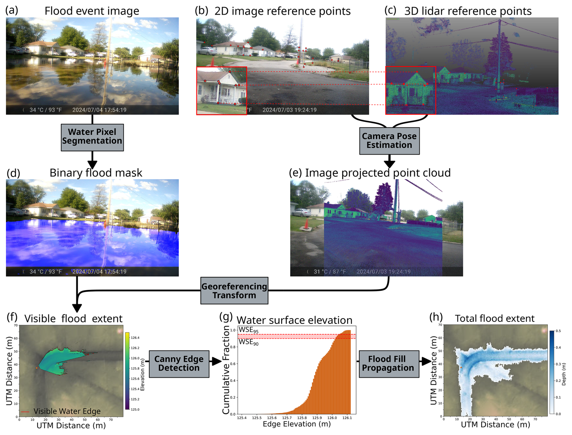
Figure 2 Procedure for estimating flood extent from a flooded image at Site B. Image and point cloud reference features are used to estimate camera pose and project points onto the image plane. The intersection with the flood mask gives the visible flood extent. Water surface elevation (WSE) is extracted from the edge elevations and propagated for the final, total flood extent.

For a given flood event, the earliest image in which flooding was visible was annotated with three to five positive point prompts. These prompts were then used to segment the remaining image sequence. The visual confirmation of flooding was used to iteratively refine the segmentation, with additional positive prompts added to correct for false negatives (i.e., flooded areas classified as non-flooded), and negative prompts added to address false positives (i.e., non-flooded areas misclassified as flooded). This process continued until flood extents were satisfactorily delineated based on visual agreement with apparent surface water boundaries. The final output of this classification procedure is a binary flood mask for each image, where pixel values of one indicate flooded regions and values of zero indicate non-flooded areas. SAM2-predicted flood masks were evaluated against manually labeled flood extents to quantify segmentation accuracy using the Intersection-over-Union (IoU) metric. IoU is defined as the ratio of true positive water-classified pixels to the total of all true positives, false positives, and false negative pixels.

In addition to spatial classification, each flood mask was used to calculate a relative measure of flood severity per image. This was quantified as the flooded pixel fraction, or the number of pixels classified as water divided by the total number of pixels in the image. This ratio is referred to as the Static Observer Flooding Index (SOFI), following the approach of Vitry et al. (2019), providing a simple proxy for flood intensity as seen from a fixed observation point. SOFI has been shown to correlate strongly with changes in water level for a given location (Moy de Vitry et al., 2019). The shape and magnitude of SOFI response depend strongly on the geometry of a camera relative flooding, and as such values cannot be directly compared between study sites.

2.5 Point cloud to image projection

The workflow for estimating floodwater elevation and extent relies on establishing a correspondence between features visible in time-lapse images and their three-dimensional coordinates within a georeferenced terrestrial point cloud. This correspondence requires knowledge of both the intrinsic parameters of each camera (such as focal length and sensor dimensions) and its extrinsic parameters, which describe the camera's location and orientation in space, referred to as the camera pose. The projection of a three-dimensional point cloud ($X,Y,Z$) in world coordinates onto a two-dimensional pixel coordinate on the image plane (u,v), is defined by Eq. (1):

$$\begin{array}{}\text{(1)}& \left[\begin{array}{c}u\\ v\\ \mathrm{1}\end{array}\right]=\mathit{K}\mathit{P}\left[\begin{array}{c}X\\ Y\\ Z\\ \mathrm{1}\end{array}\right],\end{array}$$

where

$$\begin{array}{}\text{(2)}& \mathbf{P}=\left[\mathit{R}\right|\mathit{t}].\end{array}$$

This projection is governed by two key transformation matrices: the intrinsic matrix, K, a 3×3 matrix that encodes the camera's internal geometry, including focal length and optical principal point, and the extrinsic matrix, P, which combines a rotation matrix, R, and translation vector, t, to describe the camera's pose relative to the world coordinate frame, as shown in Eq. (2). Together, these matrices enable transformation from world coordinates into image space.

Intrinsic parameters for each camera were estimated in a controlled, laboratory-based calibration using a checkerboard target with 25 mm squares printed on 216 mm by 279 mm paper. Between 20 and 30 images of the target were collected from multiple oblique angles. Collected images were processed using OpenCV, a standard computer vision library (Bradski, 2000), identifying checkerboard corners, computing the intrinsic matrix, K, and estimating a five-element distortion coefficient vector, d. This distortion matrix is used to correct projected pixel coordinates to improve accuracy of point to image projection.

The extrinsic camera pose matrix, P, was estimated based on a set of matched reference features with known locations in both image coordinates (u,v), and world coordinates ($X,Y,Z$). This process, known as the Perspective-n-Point (PnP) problem, yields an estimated camera pose denoted as P_PnP. Feature matching was performed manually, with image coordinates of reference features labeled in ImageJ (Schindelin et al., 2015) and their corresponding world coordinates annotated from the terrestrial lidar point cloud using CloudCompare (CloudCompare, 2023). Dedicate GCP installation was not possible at the study sites, and in their absence , static scene elements such as rooftops, fence posts, and utility poles were used as reference features. Between 20 and 30 such features were labeled for each camera. Point precision was limited by image resolution, point cloud noise, and the spatial resolution of the lidar scan.

Using these reference features, we estimated P_PnP using the Efficient Perspective-n-Point Camera Pose Estimation (EPnP) algorithm (Lepetit et al., 2009) as implemented in OpenCV. A random sample consensus (RANSAC) procedure was applied iteratively solve for the optimal extrinsic camera post matrix, P_PnP. For each of 10 000 random sub-samples of labeled reference points, P_PnP was computed and evaluated by its reprojection error, defined as the Euclidean distance between each labeled image coordinate (u_r, v_r), and the associated projected world coordinate of the feature (u_rp, v_rp). Points with a reprojection error exceeding 50 pixels were classified as outliers. The RANSAC iteration minimizing the number of outlier points was selected as the optimal camera pose matrix estimate, P_PnP. Accuracy of the estimated camera locations was validated by comparing the recovered camera location with the known camera position extracted from the terrestrial lidar dataset. Additional laboratory experiments were conducted to verify the performance of this workflow (Supplementary Information).

The estimated camera pose matrix, P_PnP, is initially referenced to an arbitrary, local coordinate system of the terrestrial point cloud. To enable projection from topographic coordinates into image space, P_PnP was composed with the inverse of the rigid-body transformation matrix P_GCP, obtained during georeferencing, as Eq. (3):

$$\begin{array}{}\text{(3)}& \left[\begin{array}{c}u\\ v\\ \mathrm{1}\end{array}\right]={\mathbf{KP}}_{\text{PnP}}{\mathbf{P}}_{\text{GCP}}^{-\mathrm{1}}\left[\begin{array}{c}E\\ N\\ Z\\ \mathrm{1}\end{array}\right]\end{array}$$

Equation (3) represents a final transformation pipeline that maps UTM/NADV88-referenced coordinates ($E,N,Z$) to corresponding image pixel coordinates (u,v). Using this framework, each point in the terrestrial lidar point-cloud is assigned a pixel location, enabling spatially coherent visualization and quantification of flood extent in the camera imagery (Fig. 2).

Camera post positions were stable during the case study events, however, between events camera bearing shifted by approximately 13° at Site A, and 24° at site B, requiring separate pose estimations for each event. For the moderate 14 May flood, Camera A's pose was calculated using 18 reference features, yielding a median reprojection error of 6.83 pixels. The recovered camera location was offset 46 cm from the labelled camera center in the point cloud. This apparent mismatch reflects the reduced sensitivity of reprojection error to camera position when reference features are distant or near planar, which weakens 3D positional constraints despite low pixel error. Constraining the shift in the 14 May camera position to ≤10 cm increased median reprojection errors only slightly (to 7.11 pixels). For the 4 July event, pose estimation at Camera A used 24 features, constraining camera position more effectively, resulting in a reduced camera position offset to 6 cm and a median reprojection error of 23.6 pixels. For Camera B, the 14 May pose was calculated using 22 reference features, resulting in a median reprojection error of 4.99 pixels. Due to camera movement following the lidar survey, estimated positional uncertainty can only be resolved as less than 1 m. The pose estimate at Camera B for the 4 July event used 16 reference features, yielding a reprojection error of 8.9 pixels, again with a positional uncertainty below 1 m.

2.6 Flood extent estimation

Flood extent estimation is based on the intersection of lidar-derived topography and image-derived water classifications. Using the established projection pipeline in Eq. (2), each point in the terrestrial lidar point cloud is mapped to a corresponding image pixel. If the image pixel is identified as flooded in the SAM2-derived binary segmentation mask, the associated terrestrial lidar point is classified as inundated. Because pixel resolution decreases with distance from the camera, multiple 3D points may project onto a single image pixel; therefore, all inundated points are retained and a one-to-one pixel–point correspondence is not enforced. Together, these inundated points represent the portion of the ground surface that is underwater at the time the image was captured. This set of inundated points is interpolated into a 0.05 m resolution raster representing the visible flood extent in the image. This interpolation step reduces bias associated with distance-dependent differences in point density and avoids over-representation of regions where many 3D points project to a single pixel. Water surface elevation (WSE) is estimated from the rasterized flood boundary rather than from individual pixels or raw point projections. Canny edge detection is applied to the rasterized inundation extent to identify the flood boundary, and the 90th and 95th percentiles of the resulting edge elevation distribution (WSE90 and WSE95) to account for potential topographic noise or obstruction of the water edge in the time lapse images. Assuming a flat water surface, elevations along the flood boundary should exhibit a sharp peak at the upper end of the elevation distribution. The consistency and sharpness of this peak are another parameter useful to evaluate the camera pose estimation, as errors in estimated camera orientation or translation produce unrealistically large elevation differences between near- and far-field water edges.

To estimate flood extent beyond the visible portion of the image, we apply an iterative flood-fill procedure to the 0.5 m-resolution USGS DTM (Wu et al., 2019; Samela et al., 2020). As the extent of the terrestrial scans at sites A and B do not overlap, the use of the aerial lidar DTM is necessary for evaluating camera predictions of flood connectivity across multiple sites. Beginning at the lowest observed elevation within the camera's field of view, adjacent terrain cells are iteratively inundated if their elevation is below the target WSE, continuing until no additional cells meet this condition. The requirement of topographic connectivity with the seed point prevents over prediction of flood extents likely with a simple elevation threshold applied to the entire domain. The area of interest for the flood-fill implementation focused on the direct area spanning the two camera locations, approximately 500 m by 250 m, to avoid propagation into unobservable areas. This approach assumes no-flow resistance and instant water propagation. The resulting inundated area is then converted into a flood depth map by subtracting the DTM elevation from the estimated WSE. Repeating this process for each timestamped image yields a time series of inundation maps at 30 min intervals and 0.5 m spatial resolution for each camera site. We perform this propagation independently for each event at each monitoring site to assess the potential variability in estimated WSE derived from monitoring sites with distinct scene geometries and fields of view.

2.7 Comparison to a pluvial flood model

Image-derived flood extents and depths were benchmarked against results from a two-dimensional pluvial flood model. This model is implemented using the Hydrologic Engineering Center's River Analysis System (HEC-RAS), configured with a “rain-on-grid” unsteady boundary condition to simulate overland water flow across an 89.6 km² model domain covering the study site (USACE, 2024b). The base terrain is the 0.5 m USGS DTM. Rainfall records defined the unsteady inputs the model domain, assuming spatially uniform precipitation. Water movement is governed by the diffuse-wave approximation of the shallow water equations. Initial runoff generation was calculated using the Curve Number (CN) method. For the 14 May 2024, flood event, precipitation inputs were sourced from the station at St. Louis Downtown Airport (NWS:KCPS), approximately 6 km from the site. For the 4 July 2024, event, rainfall records from the USACE Mississippi River Station (USACE:ENGM7), located 8 km away, were used. Storm drain locations and connectivity assumptions are based on a survey by the Illinois Department of Natural Resources (IDNR, 2023; HeartLands Conservancy, 2023). Model roughness and CN values are informed by National Land Cover Database (NLCD) (USGS, 2023) classifications and refined using road and building footprint data (Illinois State Water Survey, 2018). Model outputs were generated at the same spatial and temporal resolution as the image-derived flood datasets to enable direct comparison. Although image data informed general model development and guided model tuning, no direct, quantitative calibration against the imagery was performed. Further details on the development of the HEC-RAS model are included in the Supplementary Information.

To compare modelled and image-derived flood extents across consistent spatial scales, analyses were conducted at two levels: the neighborhood study area and the individual fields of view (FOV) for each camera (Fig. 1b). FOV for Camera A during the moderate (severe) flood are estimated to be roughly 1646 m² (1387 m²), with terrain elevations ranging from 125.74 m (125.73 m) to 126.84 m (126.84 m). For Camera B, the field of view area is estimated as 1442 m² (1360 m²) with an elevation range of 125.61 m (125.56 m) to 126.56 m (126.53 m) for the moderate (severe) flood event. Differences in the total field of view reflect a 13.1° shift in orientation at Camera A and a 23.6° shift in orientation at Camera B between flood events. These differences in spatial coverage and viewing geometry are important for interpreting agreement or disagreement between modelled and image-derived flood extents. As such, we use distinct spatial footprints areas for each model-data comparison.

Because the model itself in only qualitatively calibrated, its output is not treated as a direct validation for absolute water levels estimated from images. Instead, it characterizes similarity or divergence in flood behaviour predicted by each method. This is quantified both in terms of the relative agreement in predicted flood extent and spatial flood connectivity between the two methods. The primary metric focuses on identifying regions where both the model and camera-based approaches indicate flooding – areas of mutual agreement in predicted inundation. This shared extent is expressed as F_overlap, the ratio of the number of pixels classified as flooded by both methods to the total number of pixels classified as flooded by either. The relative underprediction and/or overprediction of each method is expressed as the fraction of camera predicted flood cells predicted by the model (F_M|C), and the fraction of model predicted flood cells predicted by the camera (F_C|M). The model domain includes areas separated from our camera sites by major roads and drainage canals. To provide a meaningful comparison between model output and our image-based methods, we spatially restricted our comparison to a region with the approximate bounds of the topographic depression containing the study neighborhood. Where flood extents overlap, we also compared modelled and observed water surface elevations and flood depths.

3 Results

3.1 Visual flood observations

Flood segmentation performed robustly across both monitoring sites and flood events. Following refinement using additional point prompts, image segmentation and classification produced accurate flood masks with strong agreement with manually labelled flood extents. For the moderate 14 May event, the mean intersection-over-union (IoU) for Site A was 91 % (range 21 %) and 93 % (range 18 %) for Site B. For the severe 4 July event, mean IoU was 90 % (range of 14 %) at Site A and 93 % (range 23 %) at Site B. Refinement prompts successfully eliminated all whole-image false positives. Most discrepancies occurred when flood waters were partially occluded (e.g., by vegetation, fences, or vehicles) or where strong reflections caused misclassification. Fuzziness in flood boundaries increased further away from the camera, as pixel ground resolution decreased (Eltner et al., 2021).

The segmented flood masks were used to quantify the spatial extent of visible flooding using the Static-Observer Flood Index (SOFI) (de Vitry et al., 2019) (Figs. 3 and 4). During the moderate 14 May event, two distinct flood pulses are observed at Site A, both with peaks in SOFI=0.04 (Fig. 3a). These pulses are separated by dry conditions where $\text{SOFI}=\mathrm{0}.$ In contrast, SOFI values at Site B were consistently non-zero, indicating persistent flood inundation for the entire duration of the observational period. Peak SOFI at Site B during the moderate event is 0.40. At both sites, the range of SOFI during the 4 July severe flood is elevated compared to the moderate flood event, reflecting a wider range of water surface elevations imaged. During the rising limb of the severe flood at Site A, SOFI increased steadily from 0.05–0.27, where it stays within a range of 0.002 for 1.5 h, before declining monotonically to 0.025 as floodwaters receded (Fig. 4a). Values are higher for the entirety of the event at Site B, with $\text{SOFI}=\mathrm{0.31}-\mathrm{0.49}.$ However, compared to Camera A, changes in SOFI during the flood event are more muted at Site B. These differences in SOFI magnitude and variability are likely driven by differences in scene geometry. At Site A, the camera is positioned farther from, and perpendicular to, the road capturing a broader view that includes a resident's lawn in the foreground (Figs. 3b and 4b). In contrast, Site B's camera has a tighter field of view focused exclusively on the road surface (Figs. 3c and 4c). Although flooding begins on the road in both locations, the prominence of the roadway in Site B's imagery makes the flooding more visually dominant in the scene. These results demonstrate that SOFI provides a reliable metric for tracking relative changes in inundation at individual sites and accurately captures the timing and progression of pluvial flooding. However, a direct comparison of SOFI values between monitoring sites, and flood events, is complicated by variations in camera placement, viewing angle, and scene composition.

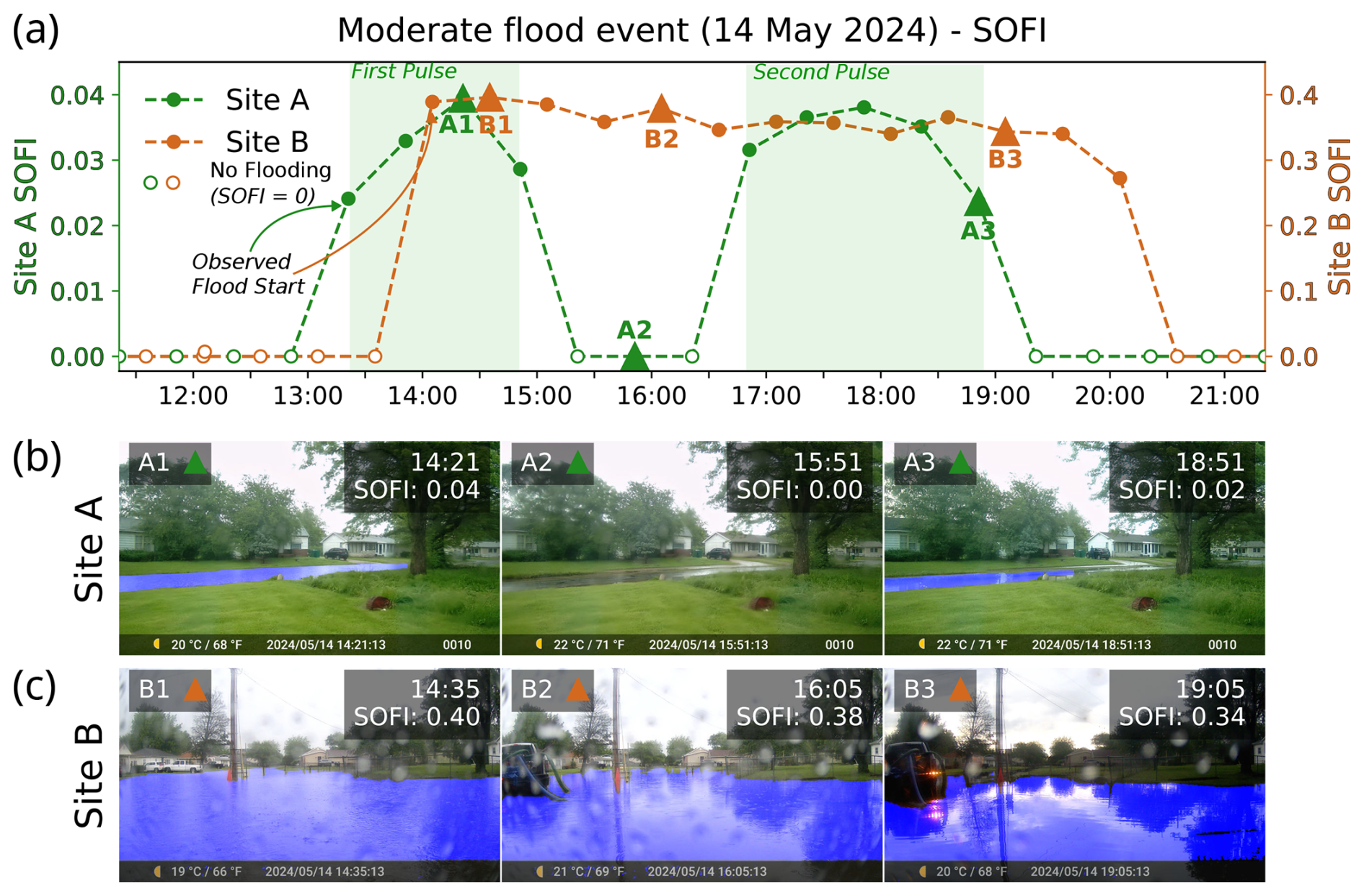
Figure 3 (a) SOFI time series for 14 May moderate severity case study event. Representative flooded images from (b) Site A and (c) Site B. Segmented flood masks are shown in blue.

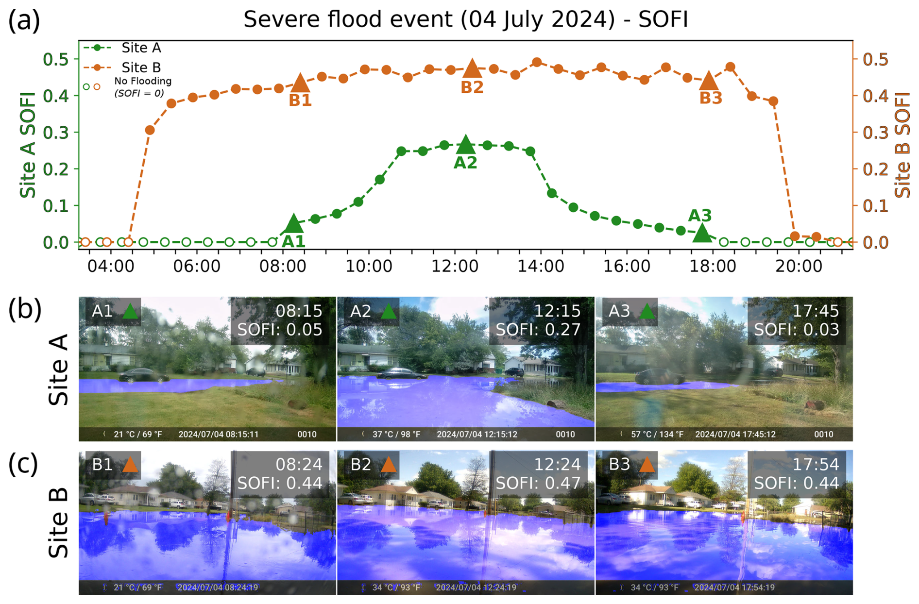
Figure 4 (a) SOFI time series for 4 July severe case study event. Representative flooded images from (b) Site A and (c) Site B. Segmented flood masks are shown in blue.

3.2 Water levels and flood extents

Using the final projection pipeline in Eq. (3), with a distortion correction applied (see Supplementary Information), water surface elevation (WSE) time series were estimated at 30 min intervals at each monitoring site for each flood event. We report both WSE₉₀ and WSE₉₅, representing the 90th and 95th percentiles of water surface edge elevations.

During the 14 May flood event, WSE₉₀ peaked twice at Site A, during each of the distinct flood pulses in the SOFI-derived hydrograph (Fig. 5a). WSL₉₀ rose from 126.00 m at the onset of visible flooding, to peaks of 126.06 and 126.04 m, separated by a period of no-flooding for all images with SOFI=0. Following the second peak, water level declines to a minimum resolved water level of WSE₉₀=125.94 m. These observations yield a range of image-derived water surface elevations of 11.3 cm. WSE₉₅ at the same site ranged from 126.02–126.13 m, peaking on the first and last images, reflecting a comparable 11.7 cm rise. In contrast, Site B experienced a broader range of water levels of approximately 34.5 cm, with ${\text{WSE}}_{\mathrm{90}}=\mathrm{125.84}-\mathrm{126.18}\mathrm{m}$), and ${\text{WSE}}_{\mathrm{95}}=\mathrm{125.88}-\mathrm{126.23}$ (range=35.6 cm), reflecting a more continuous rise and fall in water levels, rather than then distinct pulses observed at Camera A. Water levels at Sites A and B differed by a mean of 9.2 cm for WSE₉₀ and 12.8 cm for WSE₉₅, supporting the interpretation that the floodwaters occupied two disconnected patches, filling independently over the course of the event. Water level ranges for Sites A and B overlap for only a single image pair. Water level sensitivity to the elevation percentile used is similar between sites, with median ranges between WSE₉₀ and WSE₉₅ of 2.5 and 3.6 cm, for Sites A and B. Ranges between WSE₉₀ and WSE₉₅ were highest at low water levels, particularly at Site A, where maximum ranges of 13.1 and 19.0 cm occurred in the first and last images, compared to an average of 2.4 cm for the remaining images. At Site B, these ranges were generally smaller and more consistent, ranging between 1.8 and 7.6 cm, with an average of 3.9 cm.

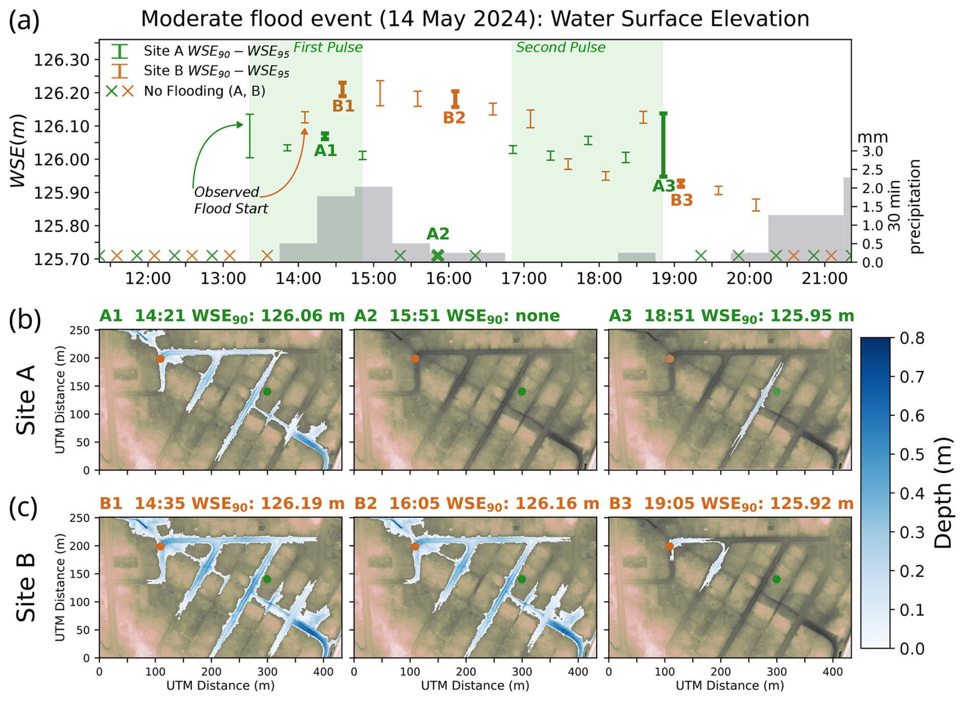
Figure 5 (a) Water surface elevations (WSE) estimated from image-lidar projection for the 14 May case study event. Flood-fill extents propagated from WSE₉₀ at (b) Site A and (c) Site B.

During the more severe 4 July flood, water surface elevations rose substantially at both sites, characterized by clearly defined rising and falling limbs in both the SOFI and camera-derived hydrographs (Fig. 6a). At Site A, WSE₉₀ varied by over 35.7 cm and WSE₉₅ over 27.9 cm, with peak water levels between 126.30 and 126.32 m. At Site B, both WSE₉₀ and WSE₉₅ spanned a larger vertical range of 53.2 cm, with peak levels overlapping closely with those at Site A (126.28–126.30 m), matching the peaks in the SOFI hydrograph within 30 min. The difference in maximum water surface elevations between sites were just 1.7 and 1.0 cm, strongly suggesting that floodwaters formed a single, hydraulically connected inundation zone spanning both monitoring locations. Compared to the May event, the range between WSE₉₀ and WSE₉₅ during the July flood was more consistent over time, with Site A showing a lower and more stable mean difference of 2.3 cm (range=7.9 cm), versus a mean difference of 3.9 cm (range=19.2 cm) at Site B. As in the earlier flood, uncertainty was greatest at the beginning and end of the event, when lower water levels produced a wider spread between WSE₉₀ and WSE₉₅. Water levels between sites agreed most closely on the rising limb of the flood, with WSE ranges overlapping across nearly every time step leading up to the peak. In contrast, the more gradual recession of floodwaters at Site B resulted in increasing divergence during the falling limb. Despite these discrepancies, the rate and direction of change in water level remained largely consistent between cameras.

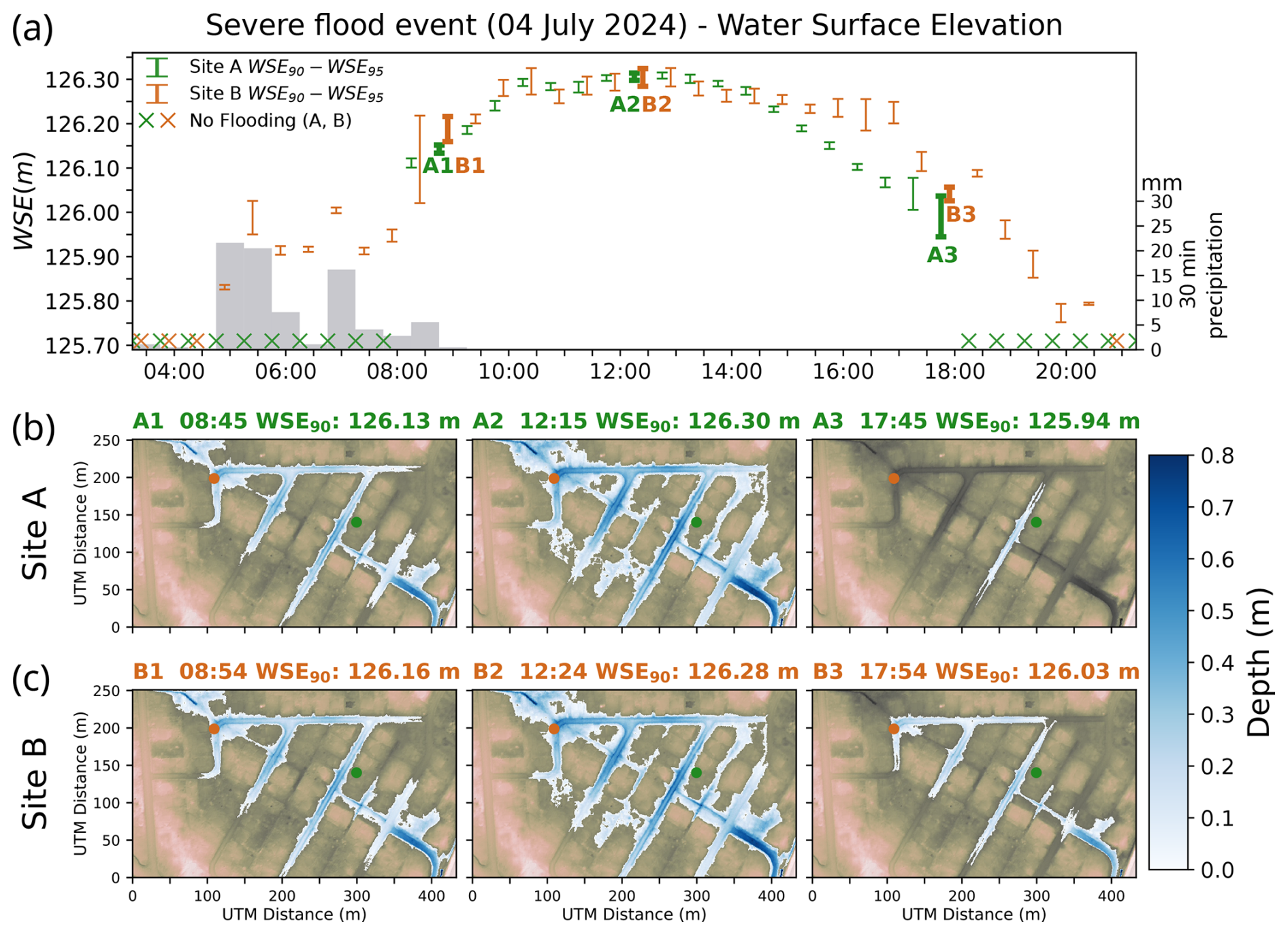
Figure 6 (a) Water surface elevations estimated from image-lidar projection for the 4 July case study event. Flood-fill extents propagated from WSE₉₀ at (b) Site A and (c) Site B.

Differences in water surface elevation between the May and July flood events directly influenced the connectivity and extent of resulting inundation, with important implications for interpreting flood dynamics. Flood-fill propagation using WSE₉₀ values from Site A produced spatially restricted inundation, with a maximum inundated area of 1.1×10⁴ m², with flooding largely confined to a patch near Camera A, only connecting to Site B at each peak in WSE₉₀ (Fig. 5b and c). In contrast, when flood-fill is propagated using the higher WSE₉₀ values from Site B, inundation extends to Site A until part way through the flood recession, including the period with no visible flooding at Site A (Fig. 5b). The resulting maximum flood extent derived from Site B WSE₉₀ was 2.0×10⁴ m², exceeding the Site A–based extent by 54.7 %. Maximum flood depths propagated using the Site B-derived hydrograph were 9.8 % greater than Site A, equivalent to 0.13 m. The maximum difference in propagated flood extents was 1.6×10⁴ m² (164 %), driven by an 11.9 cm difference in WSE₉₀ between Sites A and B. These differences resulted in a 91 cm m variation in maximum flood depth, with flood extents based on Site B's WSE₉₀ values producing inundation depths that were 102 % greater. These differences are consistent with the presence of two distinct flood pulses at Site A and a more gradual and persistent rise at Site B. The significant difference in WSE₉₀ between the sites supports the interpretation of transient connectivity, with sensitivity to threshold water levels contributing to large differences in mapped extent.

In contrast, during the 4 July flood event, peak WSE90 values at Sites A and B differed by only 1.7 cm (Fig. 6a), and flood-fill propagation from either site resulted in qualitatively similar inundation patterns (Fig. 6b and c). Both flood-fills generated a single, continuous inundation zone extending across the low-lying area between sites for most of the flood event. Propagation from Site A produced a peak extent of 3.2×10⁴ m², while propagation from Site B produced a peak extent of 3.0×10⁴ m², a difference of 6.2 %. Over the entire event, Site A and B propagated extents differed by a median of 13.9 %. At peak flood extent, this corresponds with a median expansion of the flood boundary by 0.92 m, compared to 10.9 m for the 14 May event. Differences in maximum flood depth were similarly small, and equivalent to the differences in WSE₉₀, differing by approximately 1 %. These small differences reinforce the interpretation of fully connected floodwaters spanning Sites A and B during the July event, with consistent water surface elevations driving coherent and symmetric flood propagation from either location.

3.3 Flood model comparison

Benchmarking the hydrodynamic flood model against flood-fill results shows generally good agreement in both the progression and extent of flooding, particularly during the 4 July event. Comparisons metrics F_overlap,F_M|C, and F_C|M were calculated for the peak flood extent for each event. Full confusion matrices of flood area agreement are provided in SI Fig. 6. The model successfully captures the broad dynamics of inundation, though key differences emerge in the spatial structure and timing of connectivity between flood patches. During the 14 May event, the model produces disconnected flood patches, even at peak flooding, qualitatively consistent with observations at Site A (Fig. 7a). However, the model does not capture the short period of connectivity estimated by flood-fill propagation from both Sites A and B (Fig. 7b). Of the modelled 14 May flood extent, eleven patches exceeded 100 m², accounting for 42 % of the total modelled inundated area ($A_{\text{model}}=\mathrm{0.7}\times {\mathrm{10}}^{\mathrm{4}}{\mathrm{m}}^{\mathrm{2}}$), suggesting a bias toward small, isolated flood zones. Agreement metrics for the 14 May event reflect this fragmentation (Fig. 7a and b): comparing the peak flood-fill extent based on the Site A ${\text{WSE}}_{\mathrm{90}},F_{\text{overlap}}=\mathrm{0.24}$, with modelled extent 43 % lower than the flood-fill. At Site B the total agreement between the peak flood-fill extent was similar (F_overlap=0.21), with modelled extent 63 % lower in area. The effect of these isolated patches is seen in the flood-fill extent at Site A still only covering 54 % (F_C|M=0.54) of the total model extent, but 95 % of the largest model flood patch. Similarly at Site B, F_C|M=0.64 for the full extent, and 0.99 for the largest flood patch. A similar effect is seen limiting the comparison to the camera FOV, with F_overlap increasing to 0.34 and 0.26, and F_C|M increasing to 0.88 and 0.99 for Sites A and B respectively. These spatial mismatches are accompanied by consistent underestimation in water surface elevation, with median modelled values 22 and 25 cm below WSE₉₀ at Sites A and B, respectively. Depth difference maps highlight these discrepancies, with distinct peaks aligning with the isolated modelled patches (Fig. 7c).

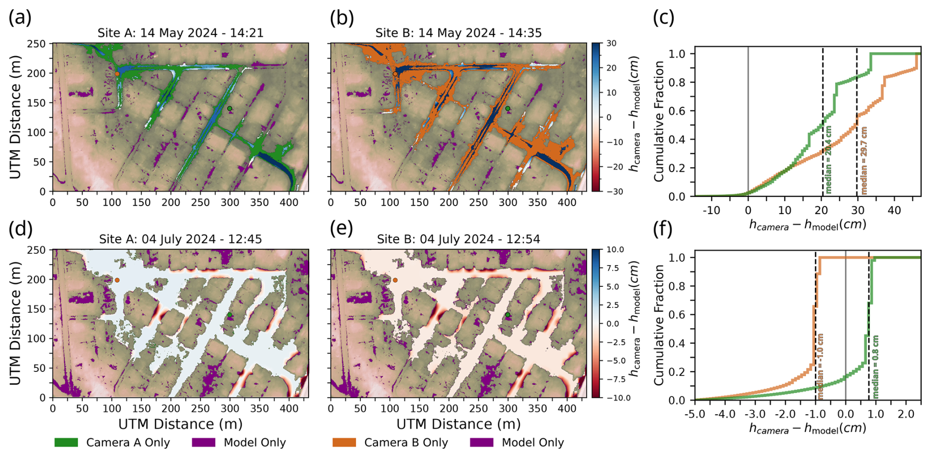
Figure 7 Comparison between peak WSE₉₀ based flood extents and HEC-RAS modelled extents for the moderate case study at (a) Site A and (b) Site B and (d, e) severe case study at Site A and Site B, respectively. (c, f) Cumulative distribution of depth differences in overlapping regions for the moderate case study and the severe case study, respectively.

In contrast, the estimated flood extents from the rain-on-grid model and our new method demonstrate significantly closer agreement for the more severe, 4 July event. At the peak of camera observed flooding, the model predicts a single contiguous flood patch, accounting for 80 % of the total modelled inundated area ($A_{\text{model}}=\mathrm{3.86}\times {\mathrm{10}}^{\mathrm{4}}{\mathrm{m}}^{\mathrm{2}}$) and connecting Sites A and B (Fig. 7d and e). Flood-fill-model agreement was also significantly higher for the 4 July event with F_overlap=0.79 and 0.77 for Sites A and B, respectively. Restricting the comparison to the within the camera FOV increases agreement to F_overlap=0.90 and 0.96 at Sites A and B, respectively. The model prediction near fully encompasses the flood-fill extents from both Site A (F_M|C=0.98), and Site B (F_M|C=1.00), while remaining isolated flood patches in the model limit flood-fill extents to 80 % (F_C|M=0.80) and 77 % (F_C|M=0.77) of model predication at each site. As with the moderate event, limiting the comparison to the largest model flood patch, increases F_C|M to 0.93 for Site A, and 0.88 for Site B. Aside from minor edge effects, the model reproduces a nearly flat water surface, with a difference of only 0.5 cm in the mean predicted water surface elevation within the camera FOV at Site A and Site B. The median water surface elevation of elevations of 126.29 m is just 1 cm below the WSE₉₀ at Site A and 1 cm above at Site B and yielding closely matched depth distributions (Fig. 7f).

4 Discussion

4.1 Strengths of Camera-Based Urban Flood Monitoring

Urban pluvial flooding is inherently shaped by subtle variations in topography, the distribution of impervious surfaces, and the configuration and performance of drainage infrastructure that regulates the spatial connectivity of floodwaters. These highly variable inundation dynamics can arise over very short distances and timescales, making them difficult to observe with other monitoring approaches. Our study demonstrated the unique strength of ground-based, time-lapse images co-registered to high-resolution topography to accurately capture these dynamics. Unlike point-based sensors or remote sensing approaches, our method directly records the spatial and temporal evolution of floodwaters, enabling high-resolution observation of disconnected, topographically-driven inundation patterns common in urban landscapes. By pairing prompted image segmentation with direct topography-to-image projection, we achieved centimeter-scale estimates of water surface elevation and time-resolved flood extents without requiring site-specific model training or in-field water-level sensors. This allowed us to quantify spatial disconnectedness during moderate and severe storm events, track changes in flood connectivity across topographic thresholds, and validate model predictions with an empirical, spatially explicit reference.

A major advantage of our workflow lies in the modularity of our processing pipeline and the relative ease of camera deployment. SegmentAnything facilitated the efficient generation of accurate flood masks for our case study images without dedicated model training. Consistent with prior work (Moghimi et al., 2024, Wang et al., 2024), we found that SegmentAnything performed robustly for floodwater segmentation, producing masks with mean IoU>90 % in most cases. However, the scalability of manual prompting for long-term automated monitoring is limited (Zamboni et al., 2025). Our new analysis workflow is agnostic to the specific source of flood masks, and future applications could easily incorporate improved segmentation techniques, either domain-specific or fine-tuned foundation models (e.g., Wagner et al., 2023), without changing the overall processing pipeline.

We found that the Static-Observer Flood Index (SOFI) provides a valuable proxy for site-specific flood dynamics inferred from an image time series, particularly during large flood events. SOFI values tracked both the qualitative progression of flooding and the image-derived WSE curves. During the 4 July severe event, SOFI rose and fell in tandem with camera-derived hydrographs at both sites, accurately capturing the timing and magnitude of inundation. However, SOFI has important limitations that constrain its broader interpretability. Because SOFI is calculated as the fraction of visible inundated area within the camera field of view, its utility is highly dependent on camera pose, viewing angle, and scene geometry. For example, SOFI at Site A reached a maximum value once floodwaters reached the edges of the frame, making the metric insensitive to further increases in water surface elevation (de Vitry et al., 2019). At Site B, SOFI also plateaued during ongoing inundation, as floodwaters extended away from the camera, decreasing pixel resolution and reducing the ability to resolve further changes in water level. This behaviour limits the comparability of SOFI values across locations or events. Accordingly, SOFI should be interpreted primarily as a scene-specific indicator of relative change in water levels over time, rather than a measure of absolute flood magnitude or spatial extent.

4.2 Water Surface Elevation (WSE) Estimation

We show that direct topography-to-image projection provides a robust basis to enable comparison of absolute floodwater levels between monitoring sites. By leveraging pre-existing features visible in the camera scenes, such as curbs, streetlight poles, and driveway edges, we were able to estimate camera pose for each event without the need for permanent ground control points or additional field surveys, even in cases where the camera had shifted slightly between floods. Our setup mirrors the likely constraints for working with images from existing public sensors, such as security cameras, that lack explicit ground control. Although the use of static scene features as GCPs can limit labelling precision and the semantic depth of extracted features, it enables scalable, repeatable deployment across heterogeneous camera networks and allows for quantitative flood observations from imagery that would otherwise be unusable for absolute measurements. In contexts requiring higher precision, the use of continuously visible, permanent ground control points (Erfani et al., 2023), fixed-mount cameras (Wang et al., 2024), or onboard inertial measurement units (IMUs) could reduce these uncertainties and allow for the reliable implementation of automated approaches. Future implementations could also integrate automated drift correction or recent advances in machine-learning-based image-to-point cloud registration (Bai et al., 2024; Jeon and Seo, 2022).

A key feature of our method is that the flood boundary identified in each image corresponds to a range of elevations, rather than a single value, likely due to slight variations in topography and minor image segmentation noise. This requires the user to select a representative elevation percentile to define the water surface elevation (WSE) for each image. In this study, we used both the 90th and 95th percentiles (WSE₉₀ and WSE₉₅) to characterize floodwater levels. Across both sites and flood events, the typical difference between WSE₉₀ and WSE₉₅ was under 5 cm, indicating consistent precision of our method within individual flood stages. Larger differences of up to 13–19 cm occurred at the very beginning and end of each flood when shallow water and fine-scale topographic noise (e.g., from curb shadows or irregular pavement surfaces) introduced greater uncertainty. These uncertainties diminished as rising floodwaters filled local topography, producing smoother and more stable elevation distributions at the floodwater edges. While isolated, noisy error in image segmentation is addressed by the spatial aggregation of edge pixels, more coherent errors, such as miss-classification of shadowed areas can systematically shift estimated water level, while maintaining narrow differences between WSE₉₀ and WSE₉₅. Despite these sources of uncertainty, our results show that extracted WSE values closely match observed inundation timing. In particular, the consistent rise and fall of WSE during the July event, most notably during the rising limb, further confirms the method's ability to resolve spatial flood dynamics at scales and frequencies that conventional sensors cannot achieve.

The contrast in water surface elevation (WSE) dynamics between the 14 May and 4 July flood events illustrates how our method captures spatial flood connectivity in urban landscapes. During the moderate 14 May event, WSE₉₀ time series at Sites A and B revealed distinct, asynchronous flood pulses, with peak elevations differing by up to 16.2 cm. Site A exhibited two short-lived pulses separated by dry conditions (SOFI=0), while Site B experienced a more continuous rise and fall in water level. These discrepancies support the interpretation that floodwaters occupied disconnected topographic depressions, each filling and draining independently in response to localized rainfall, infiltration, and drainage behavior. Our results and interpretation are consistent with similar methods that have been successfully applied to studying connectivity and surface-water flow between natural wetland depressions (McLaughlin et al., 2019). In contrast, during the more severe 4 July event, WSE time series at both sites rose and fell in tandem, with peak elevations differing by just 1.7 cm This tight correspondence in timing and magnitude of water level changes strongly indicates persistent hydraulic connectivity throughout the event. The high agreement between cameras across the full hydrograph demonstrates the value of our dual-camera system in confirming both the onset and spatial extent of flooding and in identifying when and where discrete flood patches transition into a single, continuous water surface.

4.3 Flood-fill model assessment, limitations, and uncertainties

Our flood-fill propagation method, guided by WSEs estimated using our topography-to-image projection pipeline, provide a useful basis for assessing the spatial extent of floodwaters beyond the image frame. Flood-fill approaches offer a relatively simple, computationally efficient method for exploring surface water connectivity across complex urban topography. In both natural and engineered landscapes, surface water connectivity is governed by the size, depth, and arrangement of topographic depressions and their associated spill point thresholds, which control the extent of flooding (Leibowitz et al., 2016; Samela et al., 2020; Maksimovic et al., 2009; Lee et al., 2023). Like other “bathtub models”, this approach assumes zero flow resistance and instantaneous water propagation, leading to highly non-linear relationships between water surface elevation and inundated flood area (Sanders et al., 2024). Flood fill methods are well-suited for short duration pluvial events in low relief, urban areas. Because the study sites within a self-contained depression, it is unlikely that there are substantial gradients in water surface elevation. This is supported by the 2D model results which, exclusive of edge effects, predicts a difference in water elevation between Sites A and B of only 0.5 cm after initial merging of the flood patches. Static elevation-based methods are widely used for rapid flood mapping, including in emergency management contexts (Gallien et al., 2014; Hong et al., 2024; Wang et al., 2024; Williams et al., 2020). The cross-camera comparison used in this study is an effective tool for identifying potential failure modes within these models. In our study area, flood-fill simulations propagated from Sites A and B reveal distinct connectivity patterns, with abrupt jumps in flooded extent when water surface elevations (WSE) reach key topographic spill points (Fig. 6a). The most prominent of these occurs at ∼126.01 m, where just a 2 cm increase in WSE, from 125.99 m (Fig. 8b and d) to 126.01 m (Fig. 8c and e), results in a 390 % increase in flood area at Site A and 270 % at Site B. Above this threshold, water surface elevation increases at both sites is identical, indicating that the two sites are fully hydraulically connected.

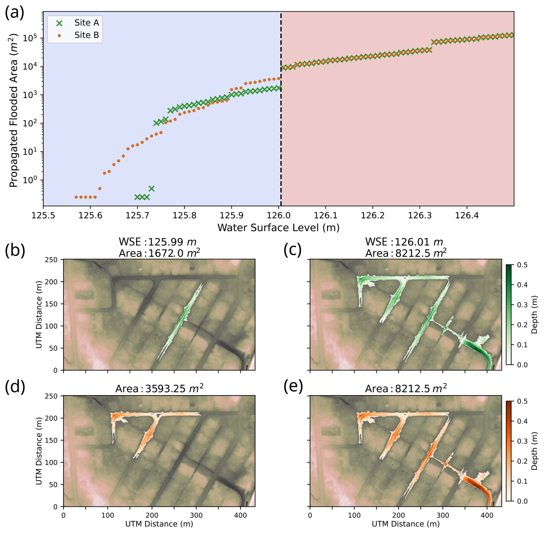
Figure 8 (a) Flood-fill-estimated inundated area as a function of WSE₉₀ for Sites A (green) and B (orange) with threshold elevation denoted with a dashed line, (b) Site A-derived flood-fill extent for WSE₉₀=125.99 m and (c) WSE₉₀=126.01 m, and (d) Site B-derived flood-fill extent for WSE₉₀=125.99 m and (e) WSE₉₀=126.01 m.

However, results from the moderate 14 May flood event reveal important limitations of the flood-fill approach for representing urban flood dynamics. Water-surface elevations derived from our topography-to-image projection show a consistent ∼10 cm difference between Sites A and B. Across a separation of only a few hundred meters, this difference provides direct empirical evidence that the flood patches remained poorly or fully disconnected throughout the event, corroborated by camera observations. Despite this, the flood-fill model predicted full connectivity because water levels at both sites exceeded the model's 126.01 m threshold, including during the observed gap in flooding at Site A. This mismatch illustrates how purely elevation-based approaches can overestimate floodwater connectivity by neglecting processes such as microtopographic barriers unresolved in the 0.5 m DEM, infiltration losses, and stormwater infrastructure that can interrupt surface flow even when spill thresholds are exceeded (Lee et al., 2023; Shrestha et al., 2022). The sensitivity of flood-fill results to DEM characteristics further limits their reliability for predictive applications. In our case, switching from a TIN to an IDW-interpolated DEM increased the predicted connectivity threshold by 4 cm, demonstrating how differences in DEM interpolation and processing alone can alter the timing and extent of predicted flood connectivity (de Almeida et al., 2018).

In contrast, our camera-derived WSE estimates directly capture the spatial and temporal behavior of floodwaters, revealing asynchronous dynamics and persistent disconnection that would otherwise be invisible to single-point or flood-fill only approaches. This 14 May, moderate flood event highlights that while flood-fill approaches remain useful for rapid flood assessment (Preisser et al., 2022), high-resolution, empirical observations are required to better constrain, validate, and improve models of flood connectivity in urban landscapes.

Elements of our method – including spatial aggregation of flood boundaries and the calculation of multiple water-level thresholds – effectively constrain uncertainty to levels suitable for urban flood characterization. We find that water-level estimates are robust to both minor random and systematic errors in flood-mask segmentation. For the severe event at Site A, water levels calculated for the half of the scene containing a parked car that partially obscured the water line differed by less than 2 cm, on average, from estimates derived from the unobstructed portion of the scene. Similarly, introducing random jitter of 10–20 pixels to the flood-mask boundary produced mean water-level differences of less than 2 cm. More substantial errors in flood segmentation or camera pose that are not mitigated by the method are typically identifiable through diagnostic artifacts, including large reprojection errors, asymmetric projected flood extents, or exaggerated differences between WSE₉₀ and WSE₉₅. In addition, the visual context provided by the images allows qualitative validation against observable flood indicators such as roadway overtopping (Fig. S5 in the Supplement).

Beyond water-level uncertainty, flood-extent estimates are influenced by the quality of the underlying topographic data. Even with careful georeferencing, physical landscape change between surveys or differences in lidar point density can introduce localized elevation discrepancies. Flood extents propagated using aerial lidar tend to be biased toward overprediction because fine-scale topographic structures, such as curbs or drainage ditches, are only partially resolved. Both water-level estimation and flood-extent propagation may therefore be most sensitive at lower water levels, where small-scale topographic features exert stronger control on flood extent. Consequently, interpretations of discrete changes in flood connectivity resulting from small increases in water level should be treated cautiously. However, because the camera images directly capture the spatial distribution of floodwaters between sites, they can provide an independent observational check on modelled flood connectivity and allow clear identification of locations where modelled inundation diverges from observed flooding. Future work should further investigate how uncertainty propagates among these sources.

4.4 Integration with urban flood models

Our results highlight the potential of image-based flood monitoring to improve calibration and evaluation of urban flood models, particularly physics-based hydraulic modelling approaches (de Vitry and Leitão, 2020). While depression-based models with volume accounting and simplified inclusion of drainage systems (e.g., Maksimovic et al., 2009; Samela et al., 2020) offer a more realistic alternative to simple flood-fill, fully 2D hydrodynamic models remain the benchmark for predictive urban flood forecasting (Guo et al., 2021; Rosenzweig et al., 2021). Recent advances in urban flood modelling have expanded the capabilities of 2D hydrodynamic models through features such as Rain-on-Grid water input and coupling with 1D sewer-stormwater systems in commonly used software packages like HEC-RAS (Sañudo et al., 2020; Guo et al., 2021).These developments have enabled more realistic simulation of complex, infrastructure-mediated flood behaviour in urban settings, accounting for both overland flow and subsurface drainage. However, the utility of these models remains limited by the availability of empirical calibration data, especially for localized pluvial events where stream gauges are absent. Engineered drainage can dramatically alter flood response, with Anni et al. (2020) finding up to a 20-fold increase in modelled flood volume when stormwater losses are not included. This sensitivity is further amplified in urban areas with aging or neglected infrastructure, where drainage performance may vary over time (Shrestha et al., 2022).

Camera-based observations provide a promising avenue to address these calibration gaps. Depending on the data available and the precision required, camera-derived information could support multiple levels of model calibration. At a minimum, observations of flood presence, extent, and connectivity can serve as semi-quantitative validation of model structure and behaviour. More detailed or well-distributed camera installations could function as stream-gauge surrogates, enabling direct calibration of key model parameters such as surface roughness, stormwater capacity, or flood wave timing. These approaches could ultimately facilitate both post-event model evaluation and real-time model adjustment, bridging gaps in empirical data for urban flood forecasting.

When possible to implement, camera-derived WSEs offer a rare empirical reference for validating modelled spatiotemporal patterns of inundation. For example, these high-resolution, time-resolved observations allow for direct comparison with outputs from an uncalibrated HEC-RAS Rain-on-Grid simulation of the 4 July flood event, revealing a close match in peak flood depth, timing, and extent. This proof-of-concept highlights the strong potential of integrating image-derived data into calibration workflows for 2D hydrodynamic models, particularly in high-flow scenarios where floodwaters are hydraulically connected and drainage networks are overwhelmed. Beyond event reconstruction, such observations can support real-time model updating, performance evaluation of stormwater infrastructure, and planning for flood mitigation in poorly instrumented or rapidly evolving urban settings, providing a practical, data-driven way to reduce uncertainty in urban flood simulations.

In contrast, for the more moderate 14 May event, the model underpredicted total flood extent. These discrepancies may reflect known challenges in simulating shallow, spatially variable flooding, where results are highly sensitive to initial conditions, roughness parameters, and the representation of drainage behaviour (de Almeida et al., 2018). In our case, they also stem from limitations in the flood-fill-based propagation used for comparison, which overestimated surface connectivity due to DEM resolution constraints and lack of drainage detail. The mismatch between predicted and observed connectivity for this smaller event illustrates how subtle differences in topography, infiltration, or active drainage (e.g., pumping) can lead to large differences in modelled flood extent. For example, human interventions such as pumping by the utility truck at Site B during our moderate flood event are immediately apparent in camera images and may give context to the rate of flood recession that would be absent from rain-on-grid model output, or pressure-based water level loggers.

Despite these challenges, our results demonstrate how empirically-derived WSEs can complement and strengthen traditional hydraulic modelling workflows. Our method provides continuous, high-resolution estimates of water level and extent that are directly tied to real flood behaviour, capturing sub-decimeter changes in WSE and floodwater connectivity that would otherwise be missed by point-based flood monitoring and modelling approaches. While further validation of camera-derived extents would be necessary for direct model calibration, this level of precision is valuable for the initial validation of uncalibrated models, an important tool for preliminary flood-risk analysis in settings with no gauges or rapidly changing infrastructure performance. As stormwater systems become increasingly strained by climate extremes, integrating data-driven camera networks with physically-based modelling frameworks offers a promising pathway for improving urban flood forecasting, response, and planning.

4.5 Community-based and practical applications

The need for actionable urban flood data is greatest in underserved communities where existing monitoring is limited, and deficiencies in large-scale flood-risk assessments often go unnoticed (Schubert et al., 2024). Closing these gaps in flood risk assessment requires empirical flood observations at scales ranging from individual streets to specific properties. Our project, conducted in coordination with Cahokia Heights residents, offers a practical solution towards the development, deployment and operation of a low cost, camera-based flood monitoring system. The design of any community-based monitoring project must balance both technical requirements and measures to protect the privacy of and minimize intrusiveness to residents (de Vitry et al., 2019; Azizi et al., 2022).

Cameras offer a flexible, low-cost, and highly informative option for distributed monitoring in settings where flooding dynamics are poorly understood. However, even under ideal conditions image-based water level estimates are unlikely to reach the absolute accuracy of pressure-based sensors, and the sensitivity of image quality to environmental conditions make them less well suited for contexts where the consistency of measurement is paramount. When more direct public sector cooperation is possible, storm drain installed pressure sensors have proven highly valuable for real time distributed flood monitoring (Gold et al., 2023; Silverman et al., 2022). However, even in these cases, cameras can serve as important complement to non-visual sensors. Gold et al. (2023) used co-located cameras and storm-drain pressure sensors to visually identify cases where storm drain based measurements may be impaired. Another major advantage of semi-permanent cameras compared to other sources of flood images, such as public webcams, security cameras, or crowdsourced photos, is the flexibility to adapt the network while otherwise maintaining stability in observations (Helmrich et al., 2021). While camera sensors themselves are highly available, the requirement of high-resolution topographic data can still be a barrier to broader application of our methods. However, advancements such as smartphone mounted lidar, and national scale datasets such as the 3D Elevation Program (USGS, 2024) have helped to mitigate these challenges. Future research could leverage this framework to optimize camera network configuration, balancing the number and placement of ground-based cameras to maximize spatial coverage and the ability to observe flood connectivity (Negri et al., 2025; Zhao et al., 2025). Based on both our own observations and resident feedback, camera position and image settings can be readily adjusted to iteratively improve the quality of flood observations. Beyond scientific data collection, community-focused monitoring also has an important role to play in the communication of flood risk and impacts (Mydlarz et al., 2024). Specifically, visual images of street-level flooding provide a tangible and easily interpretable data product for non-specialists compared to traditional products such as flood-frequency maps (Siegel and Kulp, 2021). To this end, camera-based flood observations can both fill critical data gaps related to urban nuisance flooding and provide communities with direct, actionable insights into the frequency and severity of pluvial flooding.

5 Conclusions

In this contribution, we present a novel, camera-based approach to urban flood monitoring that integrates time-lapse imagery with high-resolution topography to estimate water surface elevation and flood extent with centimeter-scale precision. Our method offers a flexible, low-cost solution for capturing urban flood dynamics, capturing highly localized events that are difficult to monitor with conventional tools. By combining foundation segmentation models with direct topography-to-image projection, we bypass the need for in-field water-level sensors and site-specific model training, enabling rapid deployment and scalability across sites. Our observations not only captured asynchronous flood dynamics and topographically driven differences in flood connectivity during moderate and severe flood events but also provided a rare empirical dataset for flood model intercomparison. Comparisons with flood-fill and 2D hydrodynamic models showed varied success in reproducing observed flood behaviour, highlighting the potential of our method to improve pluvial urban flood representation in risk assessments. Moving forward, this approach can enhance urban flood resilience by enabling real-time monitoring and more accurate forecasting to support emergency response and infrastructure planning. Additionally, integration of camera-based monitoring with hydrodynamic flood models can close critical data gaps in urban hydrology, improving understanding and management of complex flood processes in urban landscapes.