Interpretable feature incorporation machine-learning framework for flood magnitude estimation

Fluvial floods pose severe socioeconomic and environmental risks and are projected to change in frequency and severity in future decades. Estimating the magnitude of extreme floods remains challenging, particularly for sparse tail events. This motivates the need to identify predictors across catchments and time. Synoptic-scale weather patterns (WPs) are often more temporally persistent and predictable than local meteorological variables, such as precipitation. However, the value of weather patterns as predictors for flood magnitude estimation is not well established. This study introduces a feature incorporation machine learning framework to quantify the relative contribution of synoptic, meteorological, and catchment controls on winter peak-over-threshold (POT) flood magnitudes (≥99th percentile) in near-natural catchments across the United Kingdom (UK) benchmark network. We train Random Forest regression models for a pooled national sample and for multiple hydro-climatic regional samples. Model interpretability was examined using Shapley Additive Explanations (SHAP). Additionally, we analyze the conditional probabilities of the WPs co-occurring with flood magnitudes. Our results show that WPs associated with cyclonic low-pressure systems frequently coincide with flood magnitudes but add minimal value to their estimation. Model skill is dominated by static catchment attributes such as aridity and event-day precipitation in the UK model, with regional model variability in feature importance reflecting hydro-climatic contrasts. Our findings highlight the variability in model outcomes depending on the model structure and the choice of features. This study also offers methodological guidance for developing large-sample machine learning models for flood estimation that integrate atmospheric predictors with traditional hydro-meteorological and geographical variables across a feature incorporation framework.

1 Introduction

Fluvial floods are generated by complex interactions between atmospheric, hydrological, and land-surface processes occurring across various temporal and spatial scales (Berghuijs et al., 2019; Tarasova et al., 2023; Bertola et al., 2020; Nied et al., 2014). The predictability of these events varies significantly due to the interplay of local and large-scale drivers, and the rarity of extreme events in observational records further complicates predictive modeling (Blöschl et al., 2019; Berghuijs et al., 2019; Brunner and Slater, 2022). At the catchment scale, data on extreme flood events are even more limited, increasing uncertainty in both the physical understanding of flood generation mechanisms and the development of robust prediction frameworks (Yuan and Lozano-Durán, 2024; Sillmann et al., 2017; Tabari, 2021). Flood generation is also influenced by a combination of variables operating at different timescales. The complex mechanisms responsible for flood generation are often simplified and categorized into short-duration intense rainfall, saturated soil conditions, long-duration lower intensity rainfall, snowmelt, and rain on snow (Liu et al., 2022; Blöschl et al., 2019; Berghuijs et al., 2019; Merz and Blöschl, 2003).

While the main drivers of flood occurrence have been well studied, disentangling the relative importance of predictors across different timescales is challenging (Scussolini et al., 2024; Massari et al., 2023; Bárdossy and Filiz, 2005). This remains difficult due to the complexity and nonlinearity of flood systems and the limited availability of observed extreme event data. Emerging tools such as machine learning (ML) and explainable artificial intelligence (XAI) offer significant potential for exploring driver contributions. They have been successfully applied in hydrological studies to analyze large datasets and provide insights into the importance of flood drivers (Ley et al., 2024; Slater et al., 2025, 2024; Jiang et al., 2022; Coxon et al., 2024; van Hamel and Brunner, 2024).

Atmospheric circulation patterns are a valuable tool for exploring the relationship between floods and atmospheric conditions over a large area, such as the UK and Europe (Lavers et al., 2012, 2020; Schlef et al., 2019; Bárdossy and Filiz, 2005; Duckstein et al., 1993; Wilby, 1993; Brunner and Dougherty, 2022). Weather patterns (WPs) are static categories of atmospheric conditions defined over specific spatial and temporal scales, typically derived from meteorological variables such as mean sea level pressure (Neal et al., 2016; Lamb, 1972; Beck and Philipp, 2010). They can be distinguished from weather regimes (or types) based on their spatio-temporal scale. For example, a cyclonic low-pressure system influencing a regional area is often defined as a WP, whereas the North Atlantic Oscillation (NAO), which operates over a much larger spatio-temporal scale, represents a weather regime (Fabiano et al., 2021; Neal et al., 2016).

The MO-30 weather categorization scheme produced by Neal et al. (2016) categorizes daily synoptic-scale circulation over the United Kingdom (UK) and Europe into thirty discrete weather types. MO-30 has been widely used in previous UK focused research to identify the atmospheric circulation patterns influencing precipitation, drought, and coastal flooding (Richardson et al., 2018, 2020; Perks et al., 2023; Neal et al., 2018), to understand the atmospheric influence on temperature-related mortality (Huang et al., 2020), and to assess projected changes in WP frequency under future climate change scenarios (Pope et al., 2021; Huang et al., 2020). These WPs also underpin operational decision-support forecasting tools developed by the UK Met Office and the Flood Forecasting Centre, such as the “Decider” framework. For example, “Coastal Decider” as described in Neal et al. (2018) and “Fluvial Decider” as described in Richardson et al. (2020) link MO-30 WPs to regional extreme precipitation and coastal surge risk to highlight potential flood events at medium- to long-range lead times (Richardson et al., 2020; Neal et al., 2018; Perks et al., 2023). While the tool provides valuable insights and guidance for early warning and preparedness, relationships that directly link the WPs with catchment streamflow time-series or flood event characteristics have not been explored. Therefore, their utility in fluvial flood magnitude estimation remains unknown and presents a clear gap regarding the predictive value of MO-30 WPs for fluvial flood estimation.

Several studies have examined the relationships between atmospheric circulation, streamflow, and flooding across Europe and the United States, showing promising results (Brunner and Dougherty, 2022; Schlef et al., 2019; Duckstein et al., 1993; Wilby, 1993). Despite their promise, large-sample hydrological UK ML models have generally not incorporated synoptic-scale WPs as predictive features alongside land-surface and hydrometeorological variables, even though these features are closely interlinked (Brunner and Dougherty, 2022; Schlef et al., 2019; Prudhomme and Genevier, 2011; Duckstein et al., 1993). Previous studies have not evaluated the use of the MO-30 WPs as predictors for flood magnitude estimation within a large-sample, data-driven machine learning hydrological framework. Furthermore, to date research in this field has not adopted a modeling approach that incrementally adds features across a successive feature set framework, including the MO-30 WPs, to evaluate and quantify their relative contributions to flood estimation. This approach can provide model transparency in how models use features to make flood predictions, and provide insights into the possible physical mechanisms, feature interactions and relative importance of flood drivers.

Recent years have seen rapid developments in ML techniques that can handle non-linear interactions, large datasets, and high variability in predictors (Fleming et al., 2021; Nevo et al., 2022; Slater et al., 2024). Long Short-Term Memory (LSTM) networks have been extensively explored for predicting streamflow time-series and have proved very successful (Lees et al., 2021, 2022; Kratzert et al., 2018, 2022; Frame et al., 2022). These methods typically focus on time-series predictions and produce outputs at the daily time-step. In contrast, our approach focuses on estimating the magnitude of extreme streamflow events above the 99th percentile threshold exceedances at each site using large-sample data rather than by modeling continuous time-series data. Random Forest (RF) models have proven effective for understanding the drivers of hydrological events due to their ability to model complex, non-linear relationships and handle multiple data types while avoiding overfitting (van Hamel and Brunner, 2024; Slater et al., 2024; Jiang et al., 2022; Xu et al., 2024). RF models are an ensemble method that constructs multiple decision trees, aggregating predictions across these trees to provide robust outputs (Breiman, 2001; Cutler et al., 2012; Fawagreh et al., 2014). Prior work has employed RF and XAI tools to highlight feature importance in hydrological studies (Slater et al., 2025; Jiang et al., 2022; Xu et al., 2024). These data-driven approaches can reveal the potential drivers of extreme events and quantify their contributions to predictions (Xu et al., 2024; Mushtaq et al., 2024; van Hamel and Brunner, 2024; Coxon et al., 2024; Slater et al., 2024).

Current flood estimation research often ignores the interaction between weather patterns and hydrological variables in predicting flood magnitudes. Testing the integration of synoptic-scale features alongside meteorological and hydrological variables in a predictive framework is important, as novel and creative ways to enhance extreme flood prediction are needed. This study fills this research gap by investigating the contribution of synoptic-scale WPs, meteorological factors, and physical catchment features as drivers of winter extreme flood magnitudes in UK natural catchments, using large-sample ML RF models. In this work, we: (1) Assess the conditional probabilities of MO-30 WPs on fluvial flood days and the distributions of flood magnitudes associated with the MO-30 WPs. (2) Develop an interpretable feature incorporation framework with seven different feature sets in a large-sample ML framework to assess the influence of spatial identifiers, atmospheric circulation (WPs), catchment characteristics, and meteorological variables on flood magnitude estimation in UK natural catchments. (3) Evaluate the model performance and feature importance results for national and regional data samples.

To achieve these objectives, we trained structured RF models across nine spatial samples (the UK national model and eight predefined hydro-climatic regional models) for each of the seven feature sets, resulting in 63 model configurations in total. Each feature set represents a successive stage in the feature-incorporation framework. The national and regional models enable comparison between large-sample learning at the UK scale and more localized learning within homogeneous hydro-climatic regions. This study advances large-sample flood estimation research by integrating both atmospheric WPs and hydrological drivers and by providing physically interpretable insights from XAI analyses for extreme flood magnitudes (≥99th percentile).

2 Data and methods

2.1 Data sources

Daily streamflow (m³ s⁻¹) data between 1969 and 2021 were obtained for UK Benchmark Catchments from the National River Flow Archive (NRFA), as described in Harrigan et al. (2018). The corresponding catchment-averaged precipitation, potential evapotranspiration, and temperature variables were obtained from CAMELS-GB (Coxon et al., 2025), derived from the Met Office HadUK-Grid Climate Observations from Hollis et al. (2019). A selection of static catchment attributes for each of the catchments were obtained from Coxon et al. (2020). The full list of extracted variables and calculated antecedent precipitation totals, used to capture the influence of precipitation during previous days, is presented in Appendix Table A2.

The temporal span was chosen to maximize the availability of streamflow data for natural benchmark catchments. Benchmark catchments are minimally influenced by anthropogenic influences (Harrigan et al., 2018) and were chosen to explore the influence of the WPs as predictors, minimizing the influence of noise from anthropogenic activity. From the full set of benchmark catchments, we selected those for analysis which had at least 95 % of data for each water year (1 October–30 September), and at least 30 complete years of data. For each unique catchment, the normalization of streamflow (m³ s⁻¹) to specific discharge (mm d⁻¹) accounted for catchment size variability in the large-sample model and enhanced model generalizability.

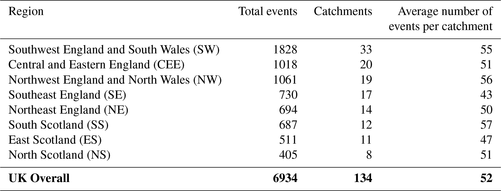
These selection criteria resulted in 134 suitable catchments. For the UK-wide analysis, all selected catchments were pooled together. For regional analysis, the catchments were grouped into their corresponding Met Office Hadley Centre Observations Dataset (HadUKP) climate regions using shapefiles (Merz et al., 2016). Region names and corresponding abbreviations (e.g., Northern Scotland = NS, Southern Scotland = SS, Central and Eastern England = CEE) are defined in Appendix Table A3. Daily WP classifications were obtained from the Met Office MO-30 dataset (Neal et al., 2016), for the same time period as the catchment streamflow data (1969–2021). These WPs were created using an annealed k-means clustering method of mean sea level pressure (MSLP) from the European Mean sea level Pressure dataset (EMSLP) (1850–2003) (Neal et al., 2016; Ansell et al., 2006). Lower-numbered WPs are associated with weaker MSLP anomalies, are historically more frequent, and occur more often in summer. Higher-numbered WPs are associated with stronger MSLP anomalies, are historically less frequent, and occur more often in winter (Neal et al., 2016). The WPs are displayed in Fig. 1, and the corresponding descriptions from Neal et al. (2016) are presented in Appendix Table A1.

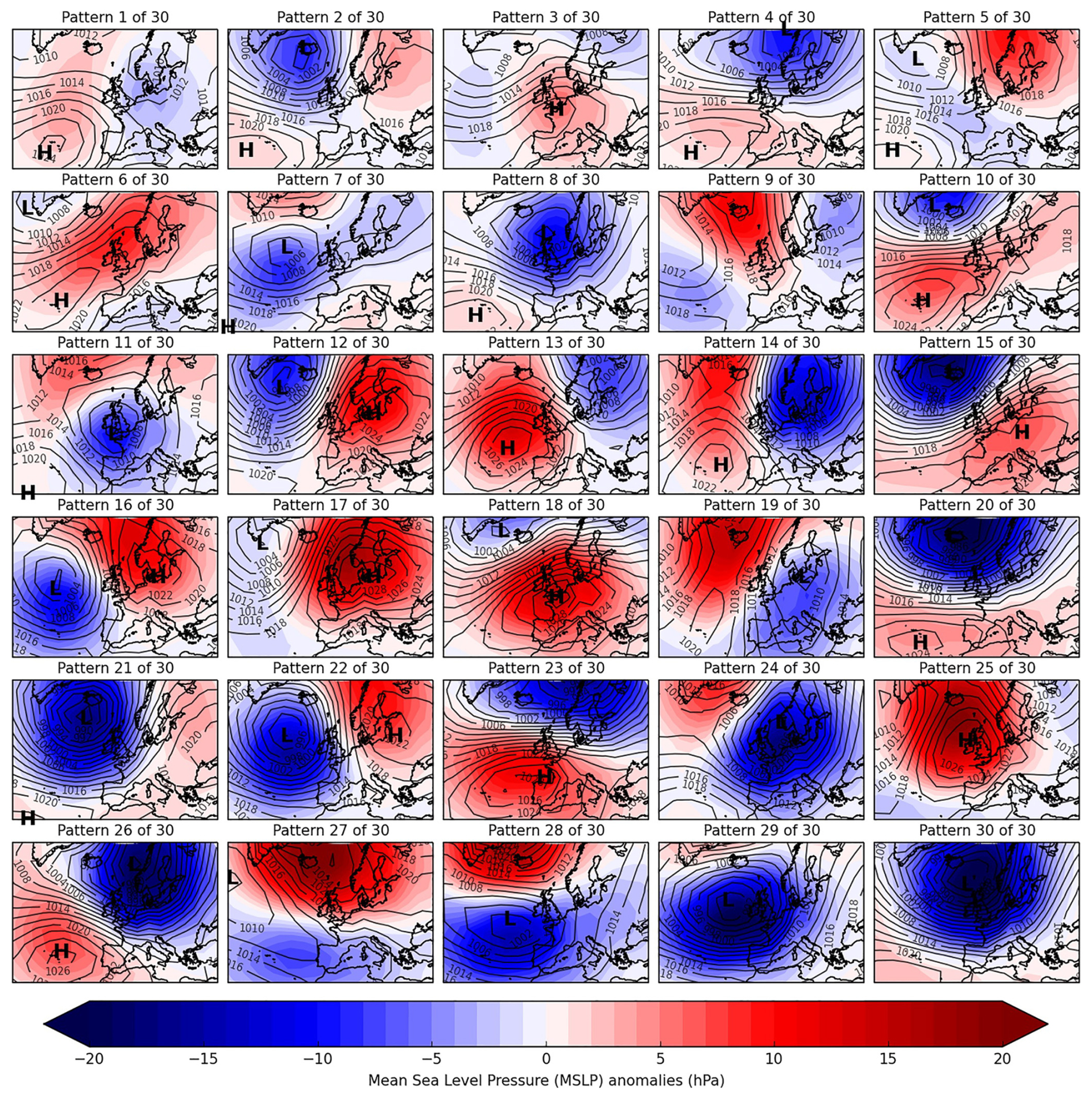
Figure 1 Weather Pattern (WP) classifications from the MO-30 dataset. From Neal et al. (2016).

2.2 Identifying flood magnitudes and dataset creation

Our analyses focus on winter floods. The winter months of December, January, and February (DJF) were chosen for analysis because most of the largest flood events in the UK occur during this season (Ledingham et al., 2019). Extreme flood events above the 99th percentile were identified for each catchment between 1969 and 2021 using the Peak Over Threshold (POT) method (Rosso, 2015; Rodding Kjeldsen and Prosdocimi, 2023). The 99th percentile threshold was used to capture the most severe events while maintaining an adequate sample size. A 7 d independence window was applied, following Brunner and Dougherty (2022). The target variable for modeling was the flood magnitude, defined as the largest specific-discharge value (mm d⁻¹) for each independent event. The resulting sample sizes and regional breakdown of catchments and independent flood events are summarized in Appendix Table A3.

Our analysis focuses on the day with the highest flood peak, defined in this study as the event-day. While this approach does not capture the full hydrograph duration, it intentionally isolates the peak magnitude of independent events. The POT method is widely recognized for its ability to capture multiple extreme events within a single year, providing a more comprehensive analysis of flood extremes compared to the Annual Maxima (AM) method (Mailhot et al., 2013; Pan et al., 2022).

For the identified flood magnitude event days, feature sets 1–6 were compiled from the datasets described above for the UK and regional samples. Feature sets include a combination of: (1) spatial identifiers (latitude and longitude), used as baseline spatial features and to provide location context for the WP classification; (2) the UK Met Office MO-30 WP category on the event day; (3) the antecedent WPs (AWPs) from one to three days prior, representing synoptic scale atmospheric conditions and pre-event circulation; (4) catchment characteristics including aridity index, area, baseflow index, streamflow elasticity, maximum elevation, and runoff ratio; (5) meteorological variables such as event-day precipitation, mean/minimum/maximum temperature, and potential evapotranspiration; and (6) antecedent cumulative precipitation for 1–3 d prior to the event, capturing short-term catchment wetness. The 3 d antecedent window was selected based on the typical response time of small, near-natural UK catchments. Overall, eight regional flood magnitude datasets in addition to the UK national dataset were produced for subsequent modeling. A summary for each region, including the number of catchments, total flood magnitude events, and mean events per catchment is presented in Appendix Table A3.

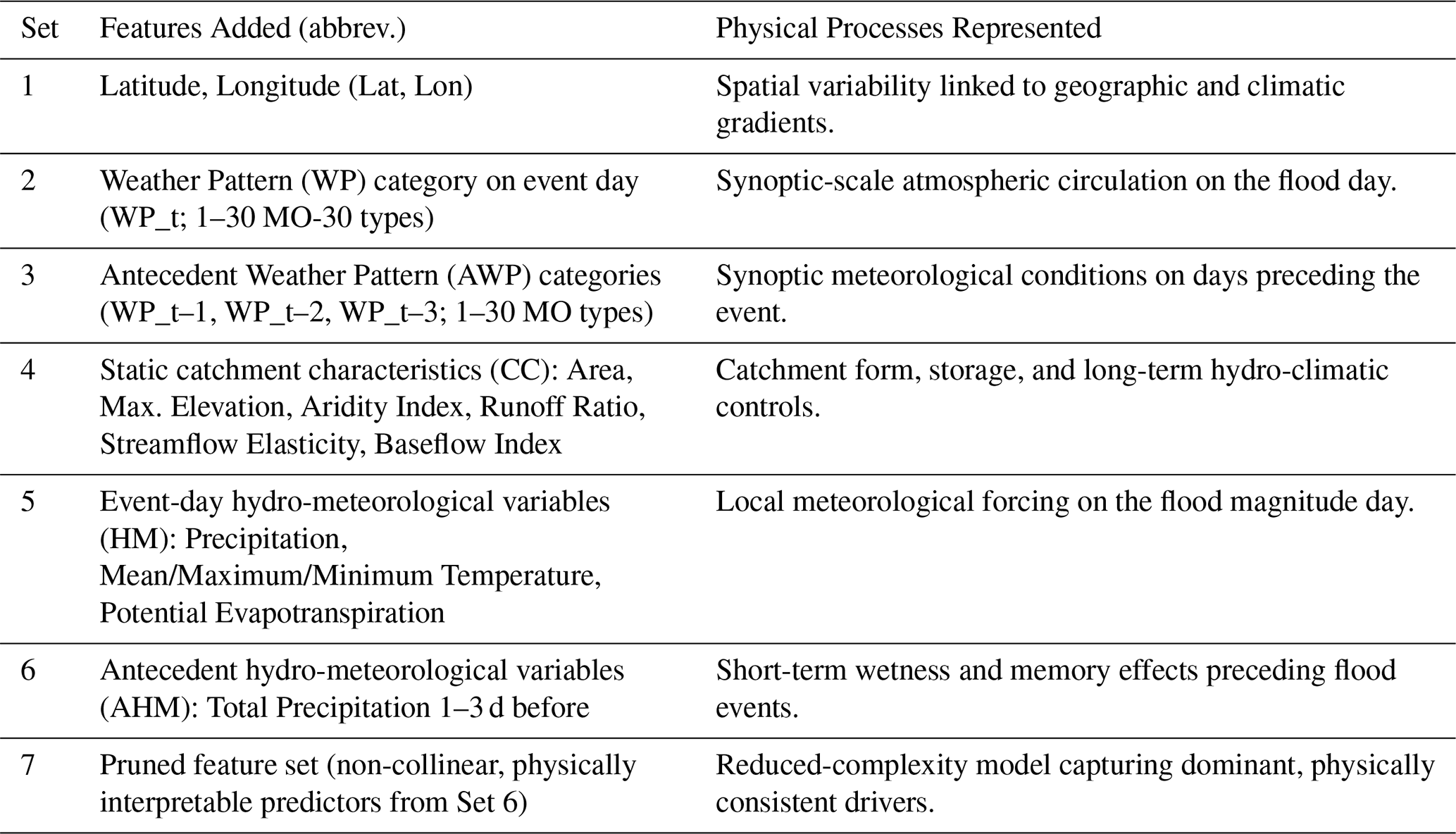
To address multicollinearity and improve the interpretability of the final feature set, a post hoc feature pruning step was applied to feature set 6 to identify the final feature set 7. Variance Inflation Factor (VIF) analysis, as described in O'Brien (2007), was used to quantify collinearity among predictors. Predictors with VIF>10 were iteratively removed, prioritizing the retention of physically interpretable variables. The final seventh pruned feature set represents the outcome of a targeted feature selection procedure applied separately to each sample (UK and regional). While feature sets 1–6 are the same across all models to allow direct comparison of process groups, feature set 7 is specific to each data sample. Consequently, the retained features differ slightly by region. Figure B1 displays the retained and dropped predictors for the UK and the 7 regional feature set models. Table 1 gives an overview of each additional feature set model, using the data sources described in Table A2, with abbreviations for model results in Fig. 4.

Table 1 Summary of the feature sets used in successive RF models. Features are added cumulatively; e.g., Set 2 includes all features from Set 1 and 2.

2.3 Conditional probabilities

Prior to selecting the WPs as a feature set for the RF models, we examined which WPs frequently occurred with extreme flood event days by computing the conditional probability of each WP given that a flood occurred on the day, denoted as “P(WP | flood)”. This analysis was performed for (1) the UK sample dataset and (2) the regional sample datasets. To account for the cumulative influence of synoptic-scale conditions leading to floods, we extended the analysis beyond the day of the event to include AWP categories (up to three days prior).

Distribution of flood magnitudes

We further explored the distribution of flood magnitudes associated with each WP, and present this for the WPs most often associated with flood magnitude days. Flood magnitude (mm d⁻¹) has already been normalized. However, since larger catchments might represent smaller flood magnitudes compared to smaller catchments, given their larger drainage areas, we present the flood magnitudes associated with each WP stratified by catchment size. To do so, the catchment sizes were categorized into lower, middle, and upper terciles (3.12–66.82, 66.82–194.81, and 194.81–1505.54 km², respectively), each containing approximately one-third of the data.

2.4 Machine learning model structure

Next, we developed seven RF regression models, each incorporating a new feature set, as described in Table 1, to gain insights into the roles of different features as predictors of extreme flood magnitudes (mm d⁻¹), for the UK and regional samples (see Table A3). The seven models were run both as a UK-wide model with all catchments pooled and for predefined regional samples (where each region has catchments within corresponding regions). This enhances interpretability by aligning the model structure with established hydro-climatic regions and enables insights into the performance and feature importance of regional and UK samples. That is, each new feature set incrementally incorporates new features, as shown in Table 1, while the model architecture remains the same. The RF was implemented using the Scikit-learn Python package by Pedregosa et al. (2011). Model performance metrics and Shapley Additive Explanations (SHAP) were calculated based on the test set results. One-hot encoding (1 = TRUE, 0 = FALSE) was applied to the WP and AWP categories to create binary features for the model. A temporal train-test split was applied to all UK and regional models, with events between 1969 and 2010 (80 %) used for training, and events from 2011 to 2021 (20 %) used for testing. This split ensured that later events were unseen during model fitting and hyper-parameter optimization. This temporal validation method has been used in other recent hydrological studies (e.g.,  Jiang et al., 2022), respects the temporal sequence of the data, and enables evaluation only on unseen years. Model hyper-parameters were optimized within the training period, using RandomizedSearchCV to balance model complexity and performance. The final configuration selected was: n_estimators = 1000, min_samples split = 10, min_samples leaf = 2, max_depth = None, and bootstrap = True. A sensitivity analysis used to test alternative tree numbers and split parameters was conducted. This also reflects a realistic forecasting scenario where future events are predicted based on past conditions (Botache et al., 2023). A three-way split (training: 1969–2000, validation: 2001–2010, test: 2011–2021) was also evaluated but produced very similar model skill. To maximize the available data for learning hydrological relationships, the two-period split was retained, providing an effective balance between robustness and data efficiency.

2.5 Uncertainty quantification

To quantify predictive uncertainty in the RF models, ensemble-based uncertainty metrics were derived from the final feature set 7 models. For each test-set sample, predictions were obtained from all individual trees within the ensemble. Two complementary metrics were employed. First, the ensemble spread of tree predictions standard deviations (Pred_SD), representing the absolute spread of predictions and thus the model's absolute predictive uncertainty in mm d⁻¹. Second, the coefficient of variation (CV), expressing the relative uncertainty. The results are presented in Fig. B2.

2.6 Test set evaluation metrics

Overall model performance was evaluated using the coefficient of determination R² and Percentage Bias (PBIAS), calculated once per model from all test set predictions of flood magnitudes. The overall R² represents the total proportion of variance in observed flood magnitudes explained by the model at the national or regional scale. For each model, R² was first calculated for the overall model and then at the catchment level. For the final 7 sets of models, comparisons were performed by re-evaluating the UK model on the exact subset of catchments used in each regional model, using identical test periods. Catchment level R² values were computed separately for each catchment and then aggregated (median and mean) across catchments within each region. Only catchments with at least ten events were included. This approach provides consistent comparisons across spatial scales and captures both temporal variation within catchments (intra-catchment variability) and variation between catchments (inter-catchment variability). The equations for R² and PBIAS are provided in Appendix C.

Significance of R² change across model generations

To evaluate the incremental effect of feature set additions on model performance, paired permutation randomized significance tests were conducted for the R² results. This method assesses whether changes in R² are statistically significant between successive model feature incorporation sets or when compared to the baseline model (feature set 1), which contains latitude and longitude. Flood event predictability inherently varies due to hydro-meteorological conditions and the physical characteristics of catchments (Brunner et al., 2021; Hakim et al., 2024), which can introduce day-to-day and catchment-to-catchment variability in model performance. This analysis was applied to each region and the UK samples for all models. By pairing predictions for the same flood events, we control for variability in event predictability, enabling robust comparisons across successive feature sets. Importantly, this approach does not assume normality, making it suitable for datasets with limited or heterogeneous samples. See the full equations in Appendix C.

2.7 Model interpretability with SHAP (SHapley additive exPlanations)

SHAP values quantify each feature’s contribution to individual predictions, providing insights into local and global influences on the target variable (Lamane et al., 2024). By applying SHAP analysis to the test sets for the 7 sets of models, model interpretability is assessed on unseen data. This approach allows for the evaluation of generalization performance and feature influence during the independent testing period. SHAP, derived from cooperative game theory, is a powerful explainable AI tool used to interpret the outputs of machine learning models (Lundberg and Lee, 2017). For each prediction in the test set, SHAP values represent the extent to which a feature contributes to deviations from the mean prediction (Wang et al., 2016; Xu et al., 2024). Compared to feature importance derived from Gini impurity, SHAP is more robust as it provides insights into both the direction and magnitude of the relationship between predictors and the target variable and enables analysis of local and global effects (Lundberg et al., 2020; Lundberg and Lee, 2017). See equations for SHAP calculation in Appendix C.

3 Results

Cyclonic MO-30 WPs have the highest conditional probabilities on winter POT flood-event days across most hydro-climatic regions and in the UK-wide sample (Fig. 2a). In the UK sample, WP 30 has the highest event-day conditional probability and occurs on 19 % of flood-event days (Fig. 2a). Other cyclonic types (including WPs 20, 21, and 29) also show elevated conditional probabilities, with regional contrasts in the most frequent WP (Fig. 2a). In North Scotland (NS), WP 23 is the most prominent event-day type and occurs on 16 % of flood-event days (Fig. 2a). Blank cells indicate region–WP combinations with no recorded flood events during the study period (Fig. 2b). Three days prior to flood events, WP 30 is less dominant than on the event day, while other higher-numbered cyclonic types (notably WPs 20 and 29) occur more frequently across multiple regions (Fig. 2b).

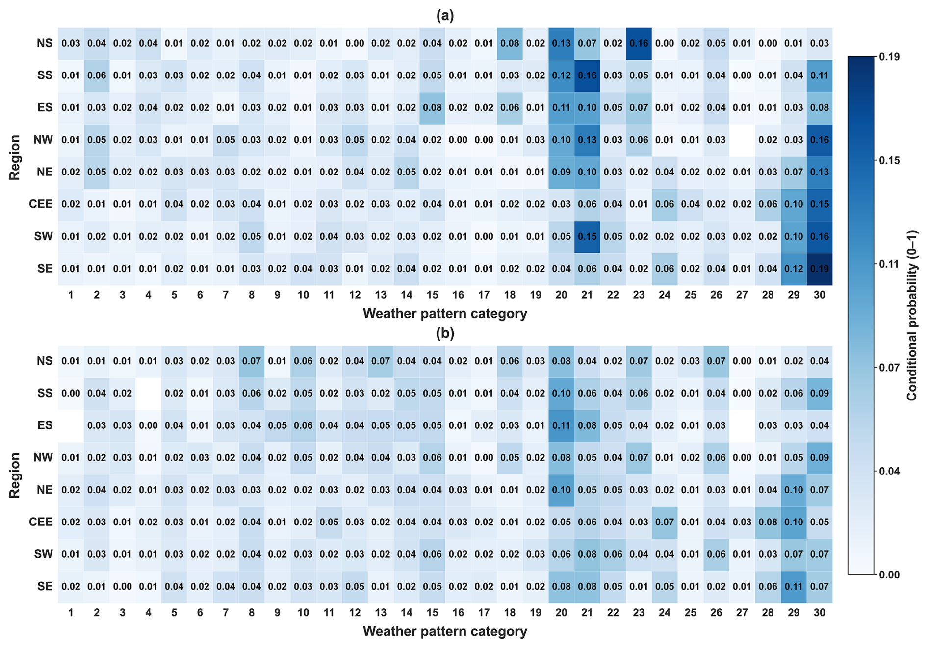
Figure 2 Conditional probabilities of WPs associated with flood days. Panel (a) shows conditional probabilities on the day of the flood, and panel (b) shows probabilities of the AWPs three days prior to the flood. Regions are indicated on the y axis (abbreviated as in Table A3) and WP categories on the x axis. The color scale represents the conditional probability value between 0 and 1, with blank cells indicating no recorded events for that region–WP combination.

Across all catchments, the distributions of winter POT flood magnitudes differ by WP, with WP 23 associated with higher typical magnitudes (higher median and mean) than the other selected patterns, while WP 30 shows a comparatively lower central tendency but a wide spread (Fig. 3a). When stratified by catchment area, small catchments exhibit the widest ranges and inter-quartile spreads in flood magnitudes for several WPs, particularly WPs 23 and 30, whereas the medium and large catchment groups show narrower distributions overall with reduced spread relative to the small catchment tercile (Fig. 3b).

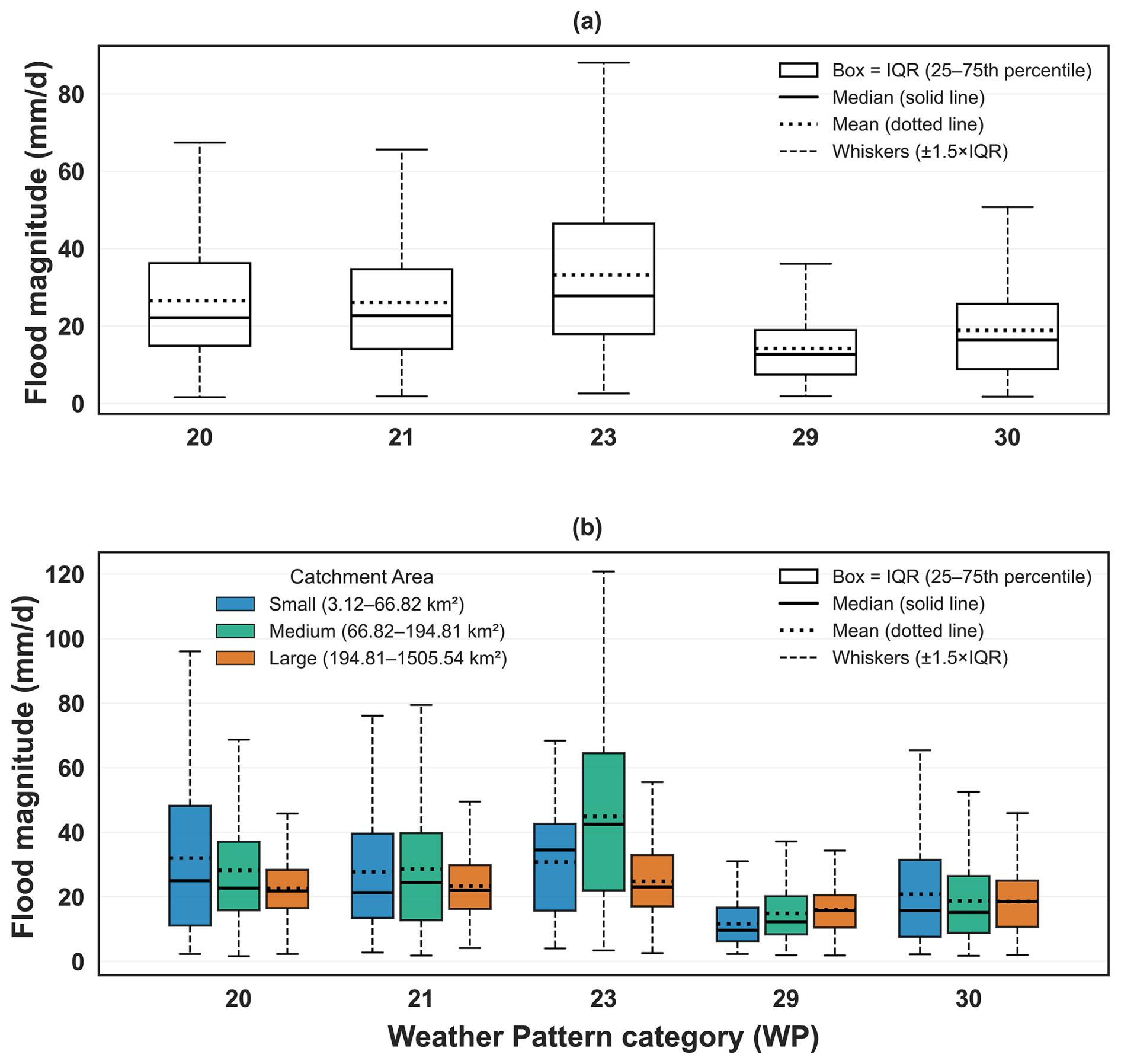
Figure 3 Comparison of flood magnitude (mm d⁻¹) distributions under selected weather patterns (WPs 20, 21, 23, 29 and 30). Panel (a) shows the distribution across all natural catchments. Panel (b) shows the distribution stratified by catchment area: Small (3.12–66.82 km²), Medium (66.82–194.81 km²), and Large (194.81–1505.54 km²). These terciles are equally sized to represent three bins of catchment area data. Boxplots show the interquartile range (IQR; Q1–Q3), the median as a solid black line, and the mean as a black dotted line; whiskers extend to 1.5 × IQR, and outliers beyond that are omitted for clarity.

The UK pooled model achieves consistently higher test-set R² values than the regional models across all feature sets, with peak performance in feature sets 6–7 (maximum R²=0.84 in set 6 and R²=0.83 in set 7) (Fig. 4a). Regional performance varies, with SW showing the highest regional R² (0.83 in set 6; 0.82 in set 7) and CEE the lowest performance (0.37 in set 6; 0.33 in set 7) (Fig. 4a). In most samples, the largest increases in R² occur when hydrometeorological predictors and antecedent precipitation indices are added (feature sets 5–6), whereas adding WP and AWP predictors (feature sets 2–3) generally does not improve R² relative to the feature set 1 baseline (Fig. 4a). Bold values with an asterisk indicate statistically significant differences in R² relative to the feature set 1 baseline (Fig. 4a). Across feature sets, PBIAS is predominantly negative in most samples for the higher feature sets, indicating a tendency to underestimate peak flood magnitudes in the test period (Fig. 4b). Bias magnitude differs by region, with the most negative PBIAS values in CEE, while NS shows comparatively positive PBIAS values (Fig. 4b).

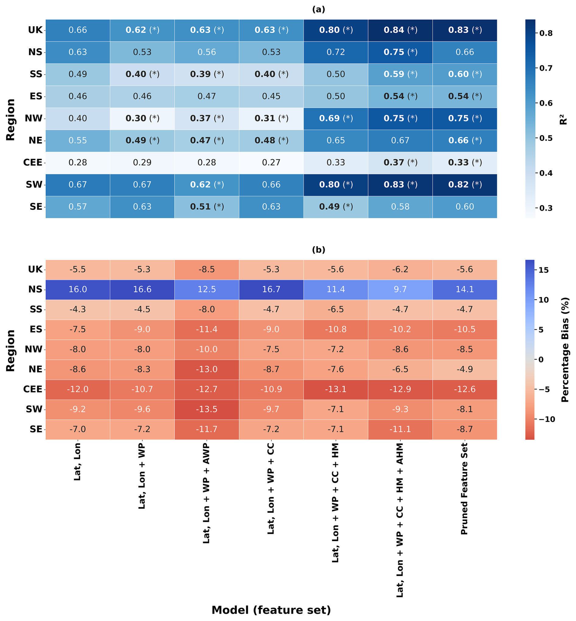
Figure 4 Comparison of UK and regional model results across model feature sets. Panel (a) shows R² and panel (b) shows percentage bias (PBIAS). In panel (a), bold values with an asterisk (*) denote statistically significant changes in R² compared to the feature set 1 models. In panel (b), blue shading indicates overestimation (positive PBIAS) and red shading indicates underestimation (negative PBIAS).

Catchment-level test-set performance shows substantial within-region variability in R² across matched catchments (Fig. 5a). Spatial differences in model skill vary by catchment, with performance contrasts captured by R² (regional minus UK) (Fig. 5b). Positive R² values (red shading) identify catchments where the regional model achieves higher R², whereas negative values (blue shading) indicate catchments where the UK model performs better (Fig. 5b). The R² performance differs between regions. The SS, ES and NW show comparatively higher median R² values, whereas CEE and SE regions exhibit lower medians and a slightly greater concentration of low-skill catchments (Fig. 5a). The head-to-head comparison indicates that differences in model skill are catchment-specific, with ΔR² (regional minus UK) varying in sign and magnitude across the country (Fig. 5b). Positive ΔR² values (red shading) identify catchments where the regional model achieves higher R², whereas negative values (blue shading) indicate catchments where the UK model performs better. The mixed pattern of red and blue points suggests that neither approach consistently dominates and that any regional-model advantage is spatially heterogeneous rather than uniform (Fig. 5b). In several regions, the distributions for the UK and regional models overlap strongly, implying that improvements from regional models are modest for many catchments but can be more pronounced for specific locations, as indicated by the tails of the R² and ΔR² distributions (Fig. 5a and b). Overall, across all matched catchments, the UK model attains higher R² more often than the regional models (54.9 % versus 45.1 %), indicating that regional modeling does not yield a consistent overall advantage despite some catchment-specific gains (Appendix Fig. B3).

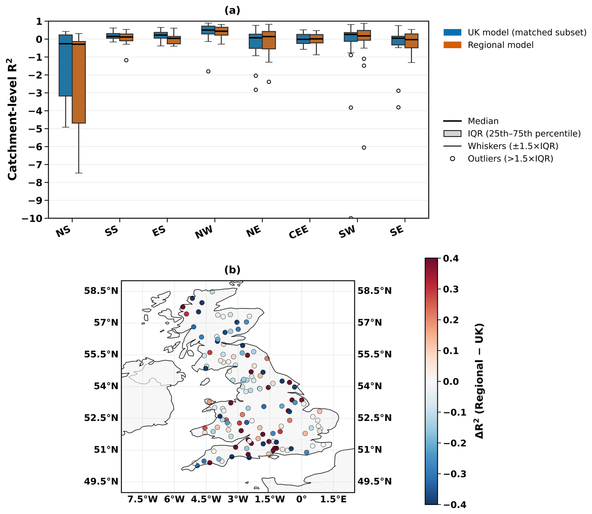
Figure 5 Comparison of UK and regional model performance at the catchment scale. (a) Boxplots of catchment R² for matched catchments across regions. Each box shows the interquartile range (IQR; 25th–75th percentile) with the median as a solid black line. (b) Spatial distribution of ΔR² differences across the UK, where red shading indicates higher performance of the regional model and blue shading indicates higher performance of the UK model.

Across the UK and regional feature set 7 models, the most influential predictors (ranked by mean absolute SHAP value) generally combine climatic context with event-scale forcing, with event-day precipitation and related antecedent precipitation indices frequently appearing among the highest-ranked variables (Fig. 6). The SHAP value distributions indicate directionality, with higher precipitation values typically associated with positive SHAP values (higher predicted flood magnitudes) and lower precipitation values associated with negative SHAP values (Fig. 6). Predictor retention and relative importance vary between regions, reflecting differences in the final pruned feature sets (Fig. 6).

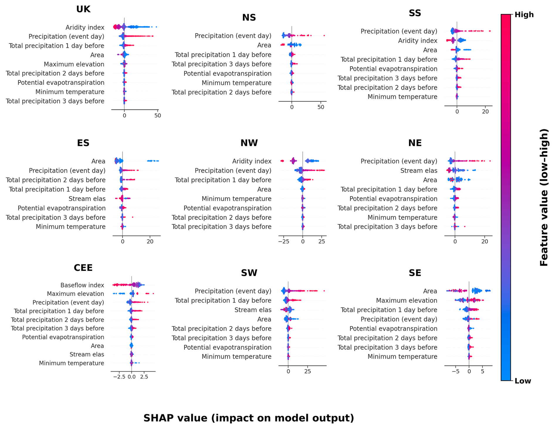
Figure 6 SHAP summary (beeswarm) plots for the UK and all regional final (feature-pruned) models (feature set 7). The number of features differs across each region. Each panel shows SHAP values representing the impact of each predictor on model output. Predictors (y axis) are ranked by their mean absolute SHAP value, with the most influential at the top. The x axis represents the magnitude and direction of each feature’s influence, where positive values indicate increased predicted flood magnitude and negative values indicate a reduction. The x axis values vary across regions. Each point corresponds to an individual prediction, with color indicating the predictor value (red = high, blue = low). Definitions and units of all variables are provided in Table A2.

Across the UK and regional feature set 7 models, the top ten predictors ranked by mean absolute SHAP ($\left|\text{SHAP}\right|$) show that the UK model is dominated by climatic context and precipitation forcing, with the aridity index as the most influential predictor, followed by event-day precipitation and antecedent precipitation indices (Fig. 7). Regional rankings show both similarities and differences relative to the UK model: precipitation-related predictors remain prominent in several regions, while some regions show a larger contribution from static catchment attributes (e.g., baseflow index, area, or elevation) among the top-ranked predictors (Fig. 7).

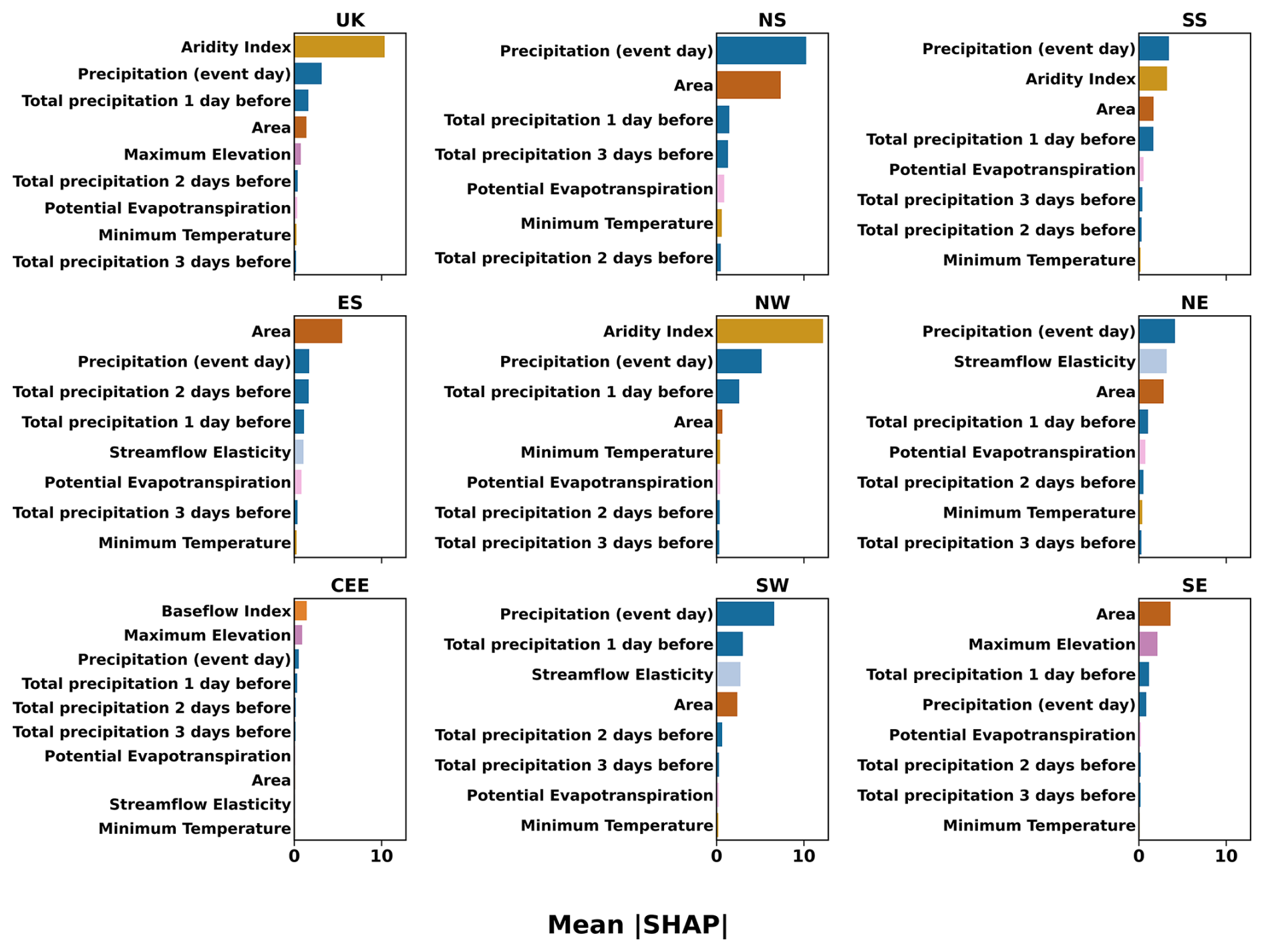
Figure 7 Final (pruned feature set 7) models. Mean absolute SHAP ($\left|\text{SHAP}\right|$) values are shown for the top ten predictors in the UK and regional feature set 7 models. Higher bars indicate stronger average influence on predicted flood magnitudes. Full variable descriptions, units, and calculation methods are listed in Table A2.

4 Discussion

4.1 Conditional probability and distribution

The dominance of cyclonic WPs on flood-event days (Fig. 2a), such as WP 30 in the UK sample, is consistent with previous work linking these synoptic regimes to enhanced UK precipitation and flooding potential (Richardson et al., 2018; Neal et al., 2018). Regional differences in the most frequent flood-associated WPs (e.g., WP 23 in NS) indicate that synoptic circulation provides a broad-scale atmospheric context. However, the resulting flood response likely depends on how that context interacts with regional hydro-climatic conditions and catchment properties (Griffin et al., 2025, 2024; Berghuijs et al., 2019). Spatial variability may also reflect differences in the precipitation footprints and storm tracks associated with individual WPs. Moreover, coastal exposure and orographic enhancement in western regions could be playing a role.

WP 21 provides an example of how frequency on flood-event days can differ from circulation types associated with widespread extreme precipitation. Previous analyses have shown that WP 21 can be associated with elevated precipitation across multiple UK regions (Richardson et al., 2018, 2020). In the present analysis, WP 21 occurs frequently on flood-event days in several regions (notably SE, SS, and NW; Fig. 2a), but WP 30 remains the most frequent type overall. This reinforces that the circulation type most strongly linked to extreme precipitation does not necessarily correspond to the type that co-occurs most frequently with flood events. This is because flood occurrence and magnitude also depend on antecedent wetness, catchment storage, and hydrological memory (Staudinger et al., 2025; Brunner and Dougherty, 2022). Consequently, the same WP can produce different flood responses in different catchments and under different pre-event conditions.

The antecedent analysis (Fig. 2b) further indicates that the synoptic context preceding flood events is not limited to the event-day circulation type. The reduced dominance of WP 30 three days prior to events, alongside more frequent occurrence of other cyclonic types (e.g., WPs 20 and 29), is consistent with the importance of multi-day circulation sequences in conditioning catchment wetness through cumulative rainfall (Berghuijs et al., 2016, 2019; Brunner and Dougherty, 2022). These results motivate the inclusion of antecedent circulation descriptors as candidate predictors in the subsequent modeling framework, while also highlighting the potential for non-linear interactions between atmospheric regime, precipitation, and catchment state.

The conditional probability patterns (Fig. 2a) provide synoptic-scale context for winter flood-event days, but the translation from circulation type to flood response is not one-to-one. The same WP can coincide with flood events more frequently in steep, fast-response catchments that are already wet, but less frequently in drier or more permeable catchments with higher infiltration capacity, reflecting the importance of antecedent wetness, storage, and hydrological memory (Staudinger et al., 2025; Brunner and Dougherty, 2022).

The antecedent analysis (Fig. 2b) indicates persistence of cyclonic circulation in the days preceding flood events. In particular, higher-numbered cyclonic types are more common three days prior to events, while WP 30 becomes less dominant and WPs 20 and 29 occur more frequently. This supports the interpretation that multi-day synoptic sequences condition catchment wetness through cumulative rainfall and soil saturation, which can increase the likelihood of flood generation (Berghuijs et al., 2016, 2019; Brunner and Dougherty, 2022).

The magnitude distributions (Fig. 3) demonstrate that WPs associated with frequent flood-event occurrences are not necessarily those associated with the highest flood magnitudes. Although WP 30 most frequently co-occurs with flood-event days (Fig. 2), it is not associated with the highest median or mean flood magnitudes (Fig. 3a). WP 30 represents a broad cyclonic regime that can persist for several days and affect large areas, which may favor frequent flood-event occurrences rather than the largest peak magnitudes (Neal et al., 2016). WP 30 could be driving lower intensity but longer duration events, especially in larger catchments where prolonged rainfall is a more important factor for flood generation, and be associated with duration rather than event peak. In contrast, WP 23 is associated with higher flood magnitudes in this event-based analysis, highlighting the importance of considering both the frequency of flood-conducive circulation types and the intensity of the flood magnitudes linked to those types (Neal et al., 2016).

Catchment size modulates these WP-magnitude relationships (Fig. 3b). Smaller catchments display wider spreads and higher upper-tail magnitudes under WPs 23 and 30, consistent with their shorter response times and sensitivity to intense rainfall. Larger catchments exhibit narrower distributions, reflecting spatial averaging and storage effects that can dampen peak responses. These differences further support that synoptic-scale regimes provide a necessary but insufficient descriptor of event-scale flood magnitude without accounting for catchment state and response characteristics.

Finally, changes in the frequency of specific circulation types could have implications for future flood hazards. For example, under RCP8.5, Pope et al. (2021) reported an increase in the occurrence of WP 23, which may be particularly relevant for regions where this WP is already prominent on flood-event days (e.g., NS; Fig. 2). This motivates future work linking circulation-type projections to hydrological impacts using predictors that better resolve catchment states and event-scale forcing.

4.2 UK and regional model performance

Feature set 7 is the final pruned specification. Latitude/longitude and WP/AWP predictors were excluded, and the remaining predictors were pruned for collinearity (Appendix Fig. B1). This means that the results for feature set 7 reflect skill attributable to the retained hydrometeorological and catchment-relevant predictors, while spatial proxies and WP/AWP categories do not contribute to (and in some regions reduce) predictive performance. A brief sensitivity check indicated that increasing model complexity did not materially change test performance, supporting the robustness of the final specification.

The UK pooled model consistently outperforms the regional models across feature sets, reaching R²=0.84 in feature set 6 and R²=0.83 in feature set 7 (Fig. 4a). The statistically significant improvement from the feature set 1 baseline (R²=0.66) is consistent with the advantages of pooling information across a larger and more diverse set of near-natural catchments, which can improve the ability of machine-learning models to learn generalizable relationships from limited extreme-event samples (Kratzert et al., 2024, 2019; Slater et al., 2024).

Across regions, model performance varies substantially, reflecting differences in dominant hydrological regimes, within-region heterogeneity, and event sample composition. The SW region achieves the highest regional performance (R²=0.83 in feature set 6; R²=0.82 in feature set 7), while the NW exhibits a large improvement relative to baseline (+0.35) reaching R²=0.75. In contrast, SS and ES show more modest improvements, reaching feature set 7 R² values of 0.60 and 0.54, respectively, consistent with the constraints of smaller regional samples.

CEE exhibited the lowest performance (R²=0.37 in feature set 6 and 0.33 in feature set 7), despite having the largest dataset. This region's low relief, permeable, and chalk dominated terrain can mean that floods are more groundwater and storage driven rather than influenced by event precipitation (Lane et al., 2019; Coxon et al., 2020). The CEE region is therefore likely less sensitive to short-duration rainfall predictors. Similarly, the SE region has low performance, reaching R² of 0.49 with hydrometeorological features and up to 0.60 by feature set 7, although this is not statistically significant compared to the baseline model (feature set 1). This aligns with previous work showing that the SE is difficult to model without explicit groundwater representation (Lees et al., 2021). These results underscore that regions dominated by slower-response processes require predictors that capture longer-term hydrological memory.

The changes in skill across feature sets highlight which predictor groups are most informative for event-scale flood magnitude estimation. In most regions, the inclusion of WP and AWP predictors (feature sets 2–3) does not improve performance relative to the spatial baseline and can reduce skill, suggesting limited incremental predictive information at daily resolution for peak magnitude estimation. This is consistent with the view that synoptic-scale circulation descriptors may not resolve the fine-scale variability associated with local precipitation extremes and catchment-scale runoff generation processes (Lavers et al., 2010). In contrast, the largest gains in R² occur once event-day hydrometeorological variables and short-window antecedent precipitation indices are included (feature sets 5–6), reinforcing the importance of forcing and antecedent wetness in conditioning peak magnitudes in many UK catchments (Blöschl et al., 2019; Berghuijs et al., 2019, 2016).

In feature set 7, performance remains similar to feature set 6 in the UK model and in several regional models, indicating that the pruning step removes redundant predictors while retaining most of the information relevant to prediction. The small reduction in R² between feature sets 6 and 7 reflects the expected trade-off between interpretability and predictive performance and supports the use of a reduced, physically interpretable predictor set for subsequent process attribution.

PBIAS results (Fig. 4b) indicate a general tendency towards the underestimation of peak magnitudes in the test period across many regions, consistent with the scarcity of observations in the upper tail and the inherent difficulty of learning extreme responses from limited event samples. NS shows comparatively smaller bias and includes cases of overestimation, suggesting region-specific differences in error structure. The largest biases in CEE co-occur with low R², further indicating that key storage-related processes are not fully represented by the current predictor set. Predictive uncertainty derived from RF ensemble spread (Appendix Fig. B2) provides additional context, with generally low median uncertainty across samples but increased uncertainty in regions with lower skill.

4.3 Catchment scale performance

Catchment-level evaluation complements pooled-scale metrics by isolating within-catchment temporal predictability in the test period. Unlike the aggregate results discussed previously, which combine inter- and intra-catchment variability across regions, this analysis calculates R² individually for each catchment based on its test events and then compares these values between the UK and the corresponding regional models. Figure 5 shows these per-catchment R² distributions, with matched comparisons between the UK and regional models. At the regional scale, the southwest (SW) maintained high aggregated R² values, but per-catchment performance revealed wide variability (ranging from −0.94 to 0.69), highlighting heterogeneity in local dynamics. This indicates that regional models can generalize well to broader regional trends but may not consistently capture localized hydrological processes driving flood magnitudes. Similar variability was observed in other regions, suggesting that model skill depends strongly on individual catchment characteristics, data density, and the distinct hydrometeorological drivers of extremes. Across all regions, the UK model outperformed regional models in 54.9 % of matched catchments (Appendix Fig. B3), confirming that large-sample pooled models generally provide stronger generalization and robustness (Kratzert et al., 2019, 2024; Slater et al., 2024).

However, regional models achieved higher performance than the UK-wide model in 45.1 % of catchments, demonstrating that locally trained models can still outperform larger models when regional hydrological characteristics are strongly distinct. Scatter-plots of per-catchment R² values in Appendix Fig. B4 show that regional models sometimes outperform the UK model, particularly in regions with coherent hydrological regimes, suggesting that local models retain value where region-specific flood processes dominate. The stronger overall UK performance reflects the model's ability to leverage greater data diversity and capture inter-catchment variability, consistent with established findings in large-sample hydrology (Kratzert et al., 2024, 2019; Slater et al., 2024). Despite this, the relatively modest catchment-level R² values in many regions highlight persistent challenges in modeling intra-catchment variability of the largest fluvial floods at the event scale. Limited extreme event records for individual catchments (often <20 events) constrain model learning and increase noise, reducing temporal prediction reliability. These data constraints likely explain some of the low or negative R² values observed in smaller or more heterogeneous catchments. Overall, this analysis reveals that while pooled UK models achieve higher generalisation, regional and catchment-specific processes still drive substantial local variability. Aggregated metrics may therefore mask poor local model skill, emphasising the importance of targeted feature engineering and model designs capable of balancing generalisation with sensitivity to local catchment dynamics.

4.4 Feature importance

Our analysis of dominant processes indicates that flood magnitude predictions are primarily controlled by a combination of climatic context, catchment features, and event-scale forcing, with aridity, catchment area and precipitation related features consistently among the most important (Figs. 6 and 7). SHAP summary plots show both the direction and magnitude of individual predictor effects on model output, whereas mean absolute SHAP values summarize the overall contribution of each predictor across all events (Figs. 6 and 7). Regional differences in predictor rankings indicate that the relative importance of climatic context, hydrometeorological forcing, and static catchment attributes varies between hydro-climatic regimes (Figs. 6 and 7).

In the highest-performing UK model, the aridity index is the most influential feature overall, followed by precipitation (event day) and cumulative precipitation on the day before. The aridity index, though static, represents a long-term control on catchment response by defining the climatic water balance under which hydrological processes operate (Coxon et al., 2020, 2025; Meira Neto et al., 2020). Lower aridity (e.g., wetter conditions) is associated with higher flood magnitudes, suggesting that catchments with persistently higher moisture availability are more efficient at converting rainfall into runoff. While the aridity index does not vary from event-to-event, its importance reflects the underlying hydro-climatic context and catchment wetness, which influence flood potential by setting the background (long-term) hydro-climatic conditions under which individual storms occur. The aridity index captures broad spatial gradients in climate and hydrology that may have previously been represented by latitude and longitude in the simpler earlier model feature sets. However, aridity provides a more physically interpretable and hydrologically meaningful descriptor of spatial variability across UK catchments.

Across both the UK and regional models, precipitation on the event day consistently emerges as a dominant predictor of extreme flood magnitudes, while antecedent precipitation plays a secondary role. In nearly all regions, the SHAP distributions confirm this behavior, with positive SHAP values associated with higher rainfall leading to higher predicted flood magnitudes. This consistency demonstrates that the models capture key physical processes, reflecting similar findings from other UK ML-based hydrological studies (Lees et al., 2021, 2022; Coxon et al., 2024).

In the SW and NW regional models, feature rankings largely mirror the UK model but reveal important regional nuances. Aridity remains a key control, but antecedent precipitation one day prior to the event gains prominence. In the SW, this could be explained by the mechanism of soil saturation and cumulative rainfall in modulating flood magnitudes (Sefton et al., 2021; Griffin et al., 2019). The SW model also attributes greater influence to topographic and temperature-related variables, consistent with elevation-driven orographic enhancement of rainfall and temperature-linked variability in evapotranspiration and antecedent wetness that together shape flood response in steep, maritime catchments (Hendry et al., 2019; Sefton et al., 2021). In contrast, lower-performing regions such as CEE and SE show a weaker dominance of dynamic predictors. Here, static features such as baseflow index, area, or elevation rank higher. This further reflects the importance of capturing slower, groundwater-influenced flood generation processes characteristic of these permeable, low-relief catchments.

Finally, while SHAP values provide valuable insight into model behavior, they represent associations rather than direct causal relationships. Non-linear feature interactions may amplify or mask underlying process signals. Therefore, SHAP-based interpretability should be used alongside physical reasoning to avoid over-interpreting model-derived relationships (Slater et al., 2025). Overall, the SHAP analysis supports that the models capture physically consistent mechanisms governing flood magnitudes, with the dominance of rainfall intensity and climatic wetness, while highlighting region-specific sensitivities to antecedent and physiographic factors.

4.5 Limitations and future recommendations

This study has several limitations that future research can address. First, uncertainty in flow observations remains a major challenge, particularly for extremes. High-flow discharge estimates are often derived by extrapolating stage–discharge rating curves beyond the range of direct gauge measurements and are sensitive to both rating curve uncertainty and stage measurement error which can be substantial during flood conditions (Horner et al., 2018; Morlot et al., 2014; Westerberg et al., 2022). In addition, the use of daily discharge can under-represent the magnitude of short-lived flood peaks because daily averaging smooths the hydrograph (Bartens et al., 2024). Future work could include quality-controlled sub-daily discharge where available to provide an improved representation of peak magnitudes (Fileni et al., 2023).

The selection of near-natural catchments was a deliberate decision to isolate natural processes; this may have reduced variability and limited the data sample size. Static features have proven to be highly important in the models, but they do not directly capture dynamic processes such as soil moisture infiltration, groundwater levels, and snowmelt. Incorporating additional dynamic variables such as snowmelt and groundwater datasets could significantly improve predictive performance in future work. Moreover, uncertainty in precipitation data also constrains model accuracy. No rainfall product will perfectly represent local conditions, and this limitation can be amplified when modeling extremes. The inclusion of WPs was motivated by their use in operational tools (e.g., Fluvial and Coastal Decider), and their potential to capture more predictable synoptic scale drivers of floods. However, despite WP-flood associations, their use in flood magnitude estimations proved limited in this study. This is likely due to a scale mismatch between the spatial resolution of the WPs and the localized behavior of flood events. Future research could aim to capture more accurately the synoptic and antecedent conditions driving floods.

Furthermore, while aggregated UK and regional metrics provide a useful overall picture, they may obscure substantial heterogeneity at the catchment scale. The lower and more variable catchment-level R² values observed in this study highlight the importance of developing multi-scale evaluation frameworks that explicitly assess local predictive skill and uncertainty. Finally, the study's deliberate design to focus exclusively on DJF events in near-natural catchments exceeding the 99th percentile threshold means that the findings represent a subset of hydrological regimes and may not fully generalize to managed or urbanized systems.

5 Conclusions

This study presents a comprehensive feature-incorporation framework for applying ML models to quantify the contributions of different predictor sets in flood magnitude estimation across natural UK catchments. By comparing feature sets consistently for a pooled UK model and multiple regional models, we quantify the extent to which different static and dynamic variables influence model performance and interpretability. The UK model achieved the highest predictive performance in the final model specifications (feature sets 6 and 7; R² 0.83–0.84), demonstrating the benefits of large-sample pooling and the diversity of training data to capture broad hydrological variability. However, catchment level evaluation showed substantial heterogeneity in skill within each region. Some catchments are predicted well, and others remain challenging for both the pooled and regional models. This variability indicates that achieving consistently high performance at local scales depends on representing fine-scale catchment properties and event-specific processes that are not fully captured by the available predictors.

This study also provides the first quantification of the limited role of the Met Office WPs in flood magnitude estimation, in this large-sample hydrological ML framework. Although cyclonic WPs are frequently associated with flood-event days, including WP and antecedent WP predictors does not improve test-set performance and can reduce skill in some regions. This suggests that, at catchment scale, WP categories provide limited additional information beyond direct hydrometeorological forcing variables. Where future work aims to understand or exploit circulation–flood linkages, improvements are more likely to come from higher-resolution circulation descriptors (e.g., moisture transport, storm-track metrics, or circulation indices tied more directly to rainfall persistence and intensity) or alternative classifications designed specifically for hydrological extremes.

SHAP-based process analysis showed that both static and dynamic hydrometeorological features were critical for estimating flood magnitudes. The aridity index was the most influential feature in the UK model. Dynamic variables, such as event day and previous days antecedent precipitation also strongly influenced flood estimation. Slower-response, groundwater-influenced regions (e.g., CEE and SE) remain more challenging to predict, underscoring the need for longer-term storage and groundwater indicators in future modeling frameworks. Future developments in flood magnitude estimation should aim to combine the generalizability of large-sample models with feature engineered processes relevant for lower performing regions. Such advances are essential for developing scalable, data-driven approaches that can inform flood risk assessment and forecasting in a changing climate. In doing this, ML models can achieve both broader applicability and enhanced predictive skill across national, regional, and catchment scales.

Appendix A: Supplementary tables

Table A1 Descriptions of the MO-30 weather pattern categories, reproduced from the dataset provided by Neal et al. (2016).

NRFA (2023)Coxon et al. (2020)Hollis et al. (2019)Coxon et al. (2025)Hollis et al. (2019)Coxon et al. (2025)Brown et al. (2023)Coxon et al. (2025)Hollis et al. (2019)Coxon et al. (2025)Coxon et al. (2020)Coxon et al. (2020)Coxon et al. (2020)Coxon et al. (2020)Coxon et al. (2020)Coxon et al. (2020)Neal et al. (2016)Neal et al. (2016)

Table A2 Variables used in the RF models.

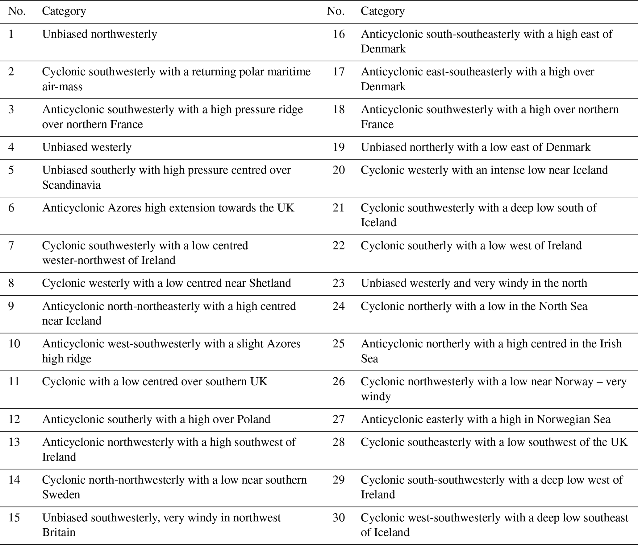
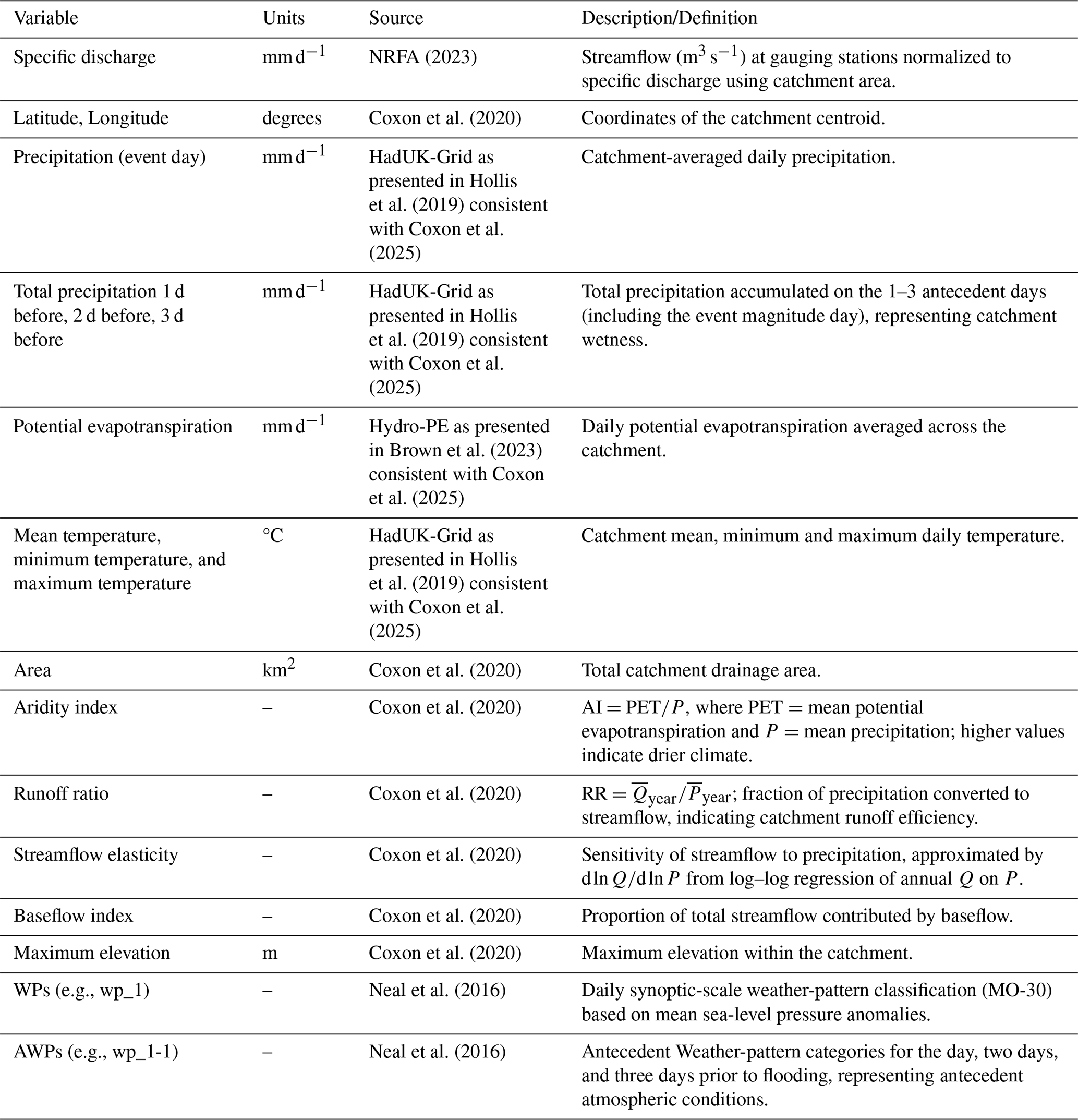
Table A3 Regional flood event summary. Regions are ordered by total event count (highest: SW; lowest: NS). Short names (e.g., “SE”) are used throughout.

Appendix B: Supplementary figures

Feature set 7 corresponds to the final pruned model specification used in the main analysis. The initial predictor pool included geographic coordinates (latitude and longitude), synoptic WPs and AWPs, static catchment attributes, hydrometeorological event-day predictors, and antecedent hydrometeorological indices. Latitude and longitude were included initially to provide spatial context for synoptic circulation (i.e., the same WP can have different hydro-meteorological implications depending on location). However, as these coordinates are not physically interpretable predictors of flood magnitude and primarily act as spatial proxies, they were removed prior to the final pruning stage to ensure that the retained predictors remained physically meaningful.

WP and AWP predictors were also removed prior to final pruning. This decision was based on model comparison results across successive feature sets (Fig. 4), which showed that adding WP and AWP predictors did not improve test-set performance relative to the baseline in most regions and, in some cases, reduced skill. Removing WP/AWP prior to collinearity pruning therefore simplified the model without loss of predictive performance, and ensured that the final specification emphasized event-scale and catchment-relevant drivers of flood magnitude.

After excluding latitude, longitude and WP/AWP predictors, variance inflation factor (VIF) pruning was applied to the remaining predictor set to reduce multicollinearity and improve interpretability. The set of retained predictors differs by region because the pruning was performed separately for each regional model. The predictors retained after pruning for each model are summarized in Fig. B1.

A sensitivity analysis was also performed to assess whether increasing model complexity affected predictive performance. In particular, model configurations with larger ensemble sizes (e.g., 2000 trees compared with 1000 trees) were tested and produced near-identical test-set performance. This indicates that the reported results are not sensitive to hyperparameter configuration, supporting the robustness of the final model specification.

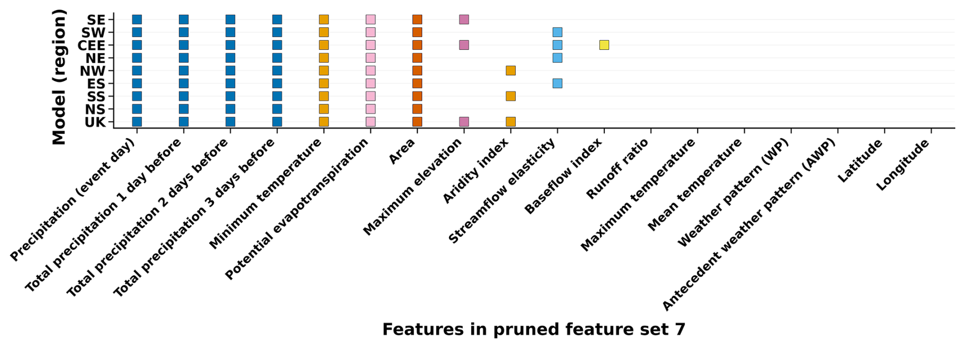
Figure B1 Feature set 7 predictors retained across UK and regional models after removal of latitude, longitude, WPs, AWPs, and then VIF pruning. Each colored square indicates that the corresponding predictor was retained in that region’s model, while blank cells denote exclusion.

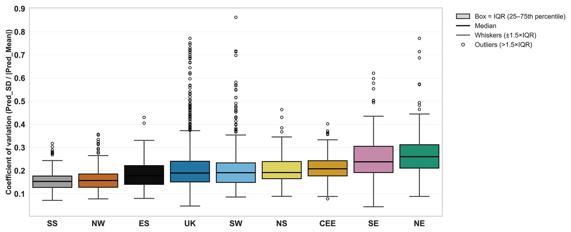
Figure B2 Ensemble-based relative uncertainty (Coefficient of Variation, CV) by region for the final feature-pruned models (Feature Set 7). The CV ($\text{CV}=\text{Pred\_SD}/\left|\text{Pred\_Mean}\right|$) rescales ensemble prediction spread by mean predicted flood magnitude, allowing comparison across regions with differing event scales. Boxes indicate inter-quartile range (25th–75th percentile), whiskers extend to 1.5 × IQR, and circles denote outliers. Lower CV values indicate higher ensemble agreement and lower predictive uncertainty. Regional models exhibit similar median CV values (≈0.15–0.25), while slightly higher uncertainty is observed in NE, SE, and NS.

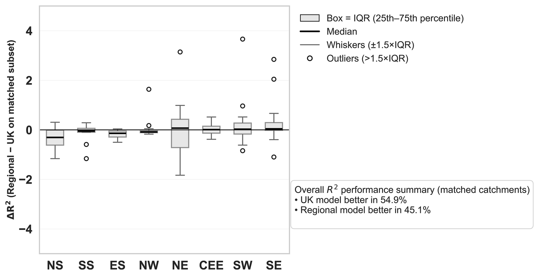
Figure B3 Per-catchment performance difference between regional and UK models (ΔR²) for matched catchments (i.e. same catchments in regional and UK models). Positive values indicate higher regional model performance. Overall, the UK model achieved higher R² in 54.9 % of catchments, while regional models performed better in 45.1 %. Boxplots show the interquartile range (IQR; 25th–75th percentile), with the median as a solid black line, whiskers extending to $\pm \mathrm{1.5}\times$ IQR, and outliers shown as points.

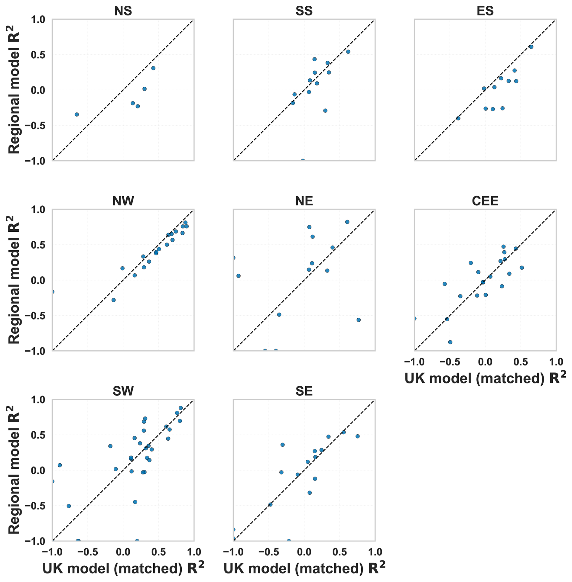
Figure B4 Scatter plots of per-catchment R² comparing UK (matched subset) and regional models for each region. Points above the dashed 1:1 line indicate catchments where the regional model achieved higher R². While the UK model generally performs better overall, regional models outperform in some areas, indicating potential benefits of region-specific model calibration.

Appendix C: Supplementary methods and equations

Uncertainty metric definition. The coefficient of variation was calculated by:

$$\begin{array}{}\text{(C1)}& \text{CV}={\displaystyle \frac{\text{Pred\_SD}}{\left|\text{Pred\_Mean}\right|+\mathit{\epsilon }}},\end{array}$$

where Pred_Mean is the ensemble mean prediction and $\mathit{\epsilon }={\mathrm{10}}^{-\mathrm{6}}$ prevents division by zero. This metric presents uncertainty as a fraction of the predicted magnitude. Appendix Fig. B2 shows the ensemble based relative uncertainty expressed as the coefficient of variation (CV) for the final pruned feature set 7 models. Median CV values across most regions fall between 0.15 and 0.25. This indicates generally good model stability and agreement among ensemble members. The SS and NW models show the lowest uncertainty, with compact inter-quartile ranges, suggesting stronger ensemble agreement in these regions. In contrast, slightly higher and more variable CV values occur in SE and NE regions, suggesting greater ensemble spread and reduced confidence in predictions. These regions also correspond to lower model skill in the main text Fig. 4, and are known to exhibit heterogeneous or groundwater-dominated hydrological responses, which may be increasing predictive uncertainty. The UK and SW models show moderate uncertainty with broader tails, likely reflecting the wider range of hydrological conditions represented in their training data. Overall, the low median CVs across all regions demonstrate that ensemble variability remains limited and that the RF models are internally stable.

Performance metrics. The equations for the performance metrics calculated on each test set per model generation are as follows:

R² (R-squared) measures the proportion of variance in actual flood magnitudes captured by the model predictions.

R² values are often reported between 0 and 1, with values closer to 1 indicating a better fit. They can also take negative values when the model performs worse than predicting the mean of the observations. R² was assessed at the national, regional, and individual catchment levels. The formula is as follows (Chicco et al., 2021):

$$\begin{array}{}\text{(C2)}& R^{\mathrm{2}}=\mathrm{1}-{\displaystyle \frac{{\sum }_{i=\mathrm{1}}^n(y_i-{\widehat{y}}_i{)}^{\mathrm{2}}}{{\sum }_{i=\mathrm{1}}^n(y_i-\stackrel{\mathrm{‾}}{y}{)}^{\mathrm{2}}}}\end{array}$$

where y_i is the observed value, ${\widehat{y}}_i$ is the predicted value, and $\stackrel{\mathrm{‾}}{y}$ is the mean of the observed values.

Percentage Bias (PBIAS) evaluates whether the model tends to overestimate or underestimate the observed values. In this definition, a negative PBIAS indicates underestimation (predictions are lower than observed values), and a positive PBIAS indicates overestimation (predictions are higher than observed values). The formula, consistent with the revised convention, is as follows (Towler et al., 2023):

$$\begin{array}{}\text{(C3)}& \text{PBIAS}={\displaystyle \frac{{\sum }_{i=\mathrm{1}}^n({\widehat{y}}_i-y_i)}{{\sum }_{i=\mathrm{1}}^n{y}_i}}\times \mathrm{100}\end{array}$$

where y_i is the observed value and ${\widehat{y}}_i$ is the predicted value.

Permutation testing for significance. Permutation testing, a non-parametric approach widely used in machine learning and environmental sciences, provides a robust framework for evaluating the statistical significance of observed effects without assuming data normality (Graham et al., 2014; Ojala and Garriga, 2010). It is particularly useful in cases with small sample sizes or heterogeneous data (Nariya et al., 2023; Graham et al., 2014).

First, for a given region, predictions for the same flood events were extracted across model generations, and the observed difference in R² between the two model generations was calculated as:

$$\begin{array}{}\text{(C4)}& \mathrm{\Delta }{R}_{\text{obs}}^{\mathrm{2}}=R_{{\text{Gen}}_{j+\mathrm{1}}}^{\mathrm{2}}-R_{{\text{Gen}}_j}^{\mathrm{2}}.\end{array}$$

To simulate the null hypothesis (H₀), which assumes no systematic difference in R², model predictions for the same flood events were randomly shuffled between the two successive feature sets. The shuffled predictions were used to recalculate R² for each feature set, and the difference was computed as:

$$\begin{array}{}\text{(C5)}& \mathrm{\Delta }{R}_{\text{shuffled}}^{\mathrm{2}}=R_{{\text{shuffled, Gen}}_{j+\mathrm{1}}}^{\mathrm{2}}-R_{{\text{shuffled, Gen}}_j}^{\mathrm{2}}.\end{array}$$

This shuffling process was repeated 1000 times to construct a null distribution of ΔR² differences. Finally, the p-value was calculated as the proportion of shuffled differences that were as extreme as or more extreme than the observed difference:

$$\begin{array}{}\text{(C6)}& p={\displaystyle \frac{{\sum }_{b=\mathrm{1}}^B\left|\mathrm{\Delta }{R}_{\text{shuffled},b}^{\mathrm{2}}\right|\ge \left|\mathrm{\Delta }{R}_{\text{obs}}^{\mathrm{2}}\right|}{B}}.\end{array}$$

If p<0.05, the observed change in R² was considered statistically significant, indicating that the feature set changes had a meaningful effect on model performance.

SHAP definition. As presented in Lundberg et al. (2020), Lundberg and Lee (2017), and Xu et al. (2024), SHAP can be explained by the following:

The SHAP value ϕ_i(f,x) for a feature x_i calculates a feature's contribution to the model’s prediction:

$$\begin{array}{}\text{(C7)}& {\mathit{\varphi }}_i(f,x)=\sum _{S\subseteq N\setminus \mathit{\left\{}i\mathit{\right\}}}{\displaystyle \frac{\left|S\right|\mathrm{!}\left(\right|N|-|S|-\mathrm{1})\mathrm{!}}{\left|N\right|\mathrm{!}}}\left(f\left(x_{S\cup \mathit{\left\{}i\mathit{\right\}}}\right)-f\left(x_S\right)\right)\end{array}$$

where ϕ_i(f,x) represents the SHAP value of feature x_i, f denotes the model’s predictive function, N is the set of all features, and S is any subset of N excluding feature x_i. Here, x_S represents the input under the given feature set S, and $\left|N\right|$ and $\left|S\right|$ correspond to the sample sizes of sets N and S.