On the relevance of molecular diffusion for travel time distributions inferred from different water isotopes

Water isotopes are a tool of choice for assessing travel time distributions of water in soils, aquifers and rivers. However, the question of whether different water isotopes tag the same travel time distributions of the water molecule, or whether the inferred travel time distribution is specific to the chosen water isotope, remains under debate. Here we conjecture that the latter is correct. We state that (a) travel time distributions of water and any tracer reflect the spectrum of fluid velocities and diffusive/dispersive mixing between the flow lines connecting the system in- and outlet, and (b) the diffusion coefficients of deuterium, tritium and ¹⁸O differ by as much as 10 %. Using particle tracking simulations, we show that these differences do indeed affect the variance of the travel time distribution – as one would expect for well-mixed advective-dispersive transport. Moreover, our simulations suggest that in the case of imperfect mixing, also the average travel time becomes sensitive to the differences in diffusion coefficients. We find that when advective trapping occurs in low conductive zones, an isotope with a smaller diffusion coefficient remains there for longer times compared to a substance exhibiting faster diffusion. This implies that for imperfectly mixed transport, average transit times ultimately increase with a decreasing diffusion coefficient: deuterium has the longest average travel time, followed by tritium, followed by ¹⁸O. Depending on the type of simulated system, we find differences in average travel times ranging from 10 d to more than 2 years. As these differences are in relative terms usually of order 5 %–10 %, one might erroneously explain them as measurement errors. Our findings suggest instead that these relative differences are physics based and may reach up to 50 % for strongly heterogeneous systems, persisting and even growing with increasing space and time scales rather than being averaged out. We thus conclude that travel time distributions inferred from O-H isotopes of the water molecule are conditioned by the chosen water isotope.

1 Introduction

Travel or transit time distributions play a key role in contaminant leaching from the partially saturated zone into groundwater (Sternagel et al., 2021; Klaus et al., 2013, 2014) and stream flow chemistry in general (Kirchner et al., 2000). As early as 1982, Simmons (1982) and Jury (1982) introduced the concept of travel time and travel distance distributions into soil physics, to acknowledge that field observations of solute transport were frequently inconsistent with predictions of the advection-dispersion model. When injecting a tracer pulse into the soil, the normalized concentration as function of depth characterizes the distribution of travel distances at a fixed time, while the time series of the normalized concentration observed at a constant depth yields the distribution of times the molecules need to travel to this depth (TTD). Recalling the theory of linear systems, Simmons (1982) and Jury (1982) advocated the TTD, also often referred to as solute breakthrough curve (BTC), as the transfer function for simulating solute breakthrough to a given depth. In line with this approach, Barnes and Bonell (1996) applied unit hydrograph techniques to predict solute transport in catchments.

The charm of this approach is that by using alternative transfer functions, one can step beyond the limitations of advective-dispersive transport. The latter is also called Fickian transport and reflects the case of perfect mixing, wherein chemical species visit the entire domain and thus experience the entire spectrum of fluid velocities “many” times. In this case, the central limit theorem applies, and normally distributed transport distances emerge and the variance in travel distances grows linearly with time (Roth and Hammel, 1996). Simmons (1982) showed that a stochastic convective transfer function is well suited to simulate solute transport in the yet imperfectly mixed near field, where the variance in travel distance grows with the squared transport time. The general drawback here is that transfer function approaches require linearity and thus a time invariant velocity field. However, water flow velocities do change nonlinearly with soil water content, which means that TTD are conditional to (changing) soil water contents and rainfall forcings. This explains notably why transfer function approaches are (despite their mathematical appeal) of low practical relevance to predict solute leaching in soils.

Strikingly, the concept of travel time distributions was used even earlier in groundwater and catchment systems as reported by Eriksson (1958) and Bolin and Rodhe (1973). Furthermore, Berkowitz and Scher (1995) introduced the continuous time domain random walk to simulate Fickian and non-Fickian transport of chemical species, which essentially uses transfer functions characterizing travel time distributions of solutes inferred from observed BTCs; see Berkowitz et al. (2006) for a detailed introduction. Naturally, travel or transit time distributions can also be defined for entire river basins (McGlynn et al., 2002, 2003; Weiler et al., 2003; Hrachowitz et al., 2009, 2016; Benettin et al., 2015, 2018; Rodriguez et al., 2018, 2021), because catchments or watersheds drain the collected precipitation to their stream outlet or release it via evapotranspiration. The defined “inlet” for rainfall and tracers is hence the catchment surface/soil surface, while the defined outlet is either the riparian zone when focusing on transit times of streamflow or the soil-vegetation system to infer transit times of evaporation and transpiration. As flow velocities in the stream are several orders of magnitude larger relative to those prevailing in the subsurface domain, tracer observations at the catchment outlet yield a very good (lumped) approximation of the transit time distribution of water and chemical species through the catchment system into the stream.

Early attempts to predict stream flow chemistry and related transit times relied also on transfer functions (Barnes and Bonell, 1996; McGuire and McDonnell, 2006) and naturally faced the same problems of state-dependent and seasonally varying travel time distributions. To overcome this problem, Hrachowitz et al. (2013) proposed using mixing coefficients, while Harmann (2015) and Rinaldo et al. (2015) introduced the concept of age ranked storage in combination with StoreAgeSelection (SAS) functions for inferring travel time distributions of stream flow. This requires the numerical solution of the Master Equation, i.e., the catchment water balance for each time and each age (Rodriguez and Klaus, 2019) alongside an appropriate selection of the functional form of SAS-function(s), e.g., as a gamma or beta distribution (Hrachowitz et al., 2011; Klaus et al., 2015; Rodriguez and Klaus, 2019; van der Velde et al., 2015) and their weights. Recent work reveals that this approach is even suited to capture fingerprints of preferential flow in the partially saturated zone (Türk et al., 2026). A closer look reveals that the use of mixing coefficients is functionally similar to the SAS approach using piece-wise linear age sampling distributions, as shown by Hrachowitz et al. (2016).

Any attempt to infer travel time distributions requires, essentially, the use of tracers; clearly water isotopes play a key role here as they provide a time-continuous source of information for this purpose at the pedon (Sprenger et al., 2016) and the catchment scales (McGlynn et al., 2002; Weiler et al., 2003; Klaus et al., 2013; Sprenger et al., 2016). Yet to date, a controversial debate prevails as to whether different water isotopes yield information on the same travel time distribution. Rodriguez et al. (2021) found different median travel times of deuterium (1.77 years) and tritium (2.19 years) in the 42 ha large Weierbach catchment in Luxembourg using an SAS approach combining three different age distribution functions. However, the authors considered these differences as unphysical, because they assign two times to “the same water molecule” and explained these differences by mere measurement uncertainty. However, Stewart et al. (2010, 2021) report that average travel times inferred from ¹⁸O and tritium might differ more than one year and argued that these differences are significant and physics based. More recent work of Wang et al. (2023) reported that the water ages and transit time distributions inferred from ¹⁸O and ³H using the SAS approach were largely consistent, while related differences appeared substantial when using a convolution model approach. Obviously, comparative studies must be very precise about their underlying methods for inferring travel times, to ensure that they are comparing the same quantities.

Here we conjecture that travel time distributions are indeed specific to the chosen water isotope. More specifically, we argue that (a) TTDs reflect the spectra of fluid velocities along the flowlines of variable lengths as well as diffusive and/or dispersive mixing among them, and (b) the diffusion coefficients of deuterium (D₂O or HDO), tritium (HTO) and ¹⁸O (¹⁸OH₂) differ by as much as 10 %. At the pore scale, one would thus naturally expect differences, as the underlying transport process is essentially advective-diffusive. At larger scales, one can observe either Fickian or non-Fickian transport. Fickian transport reflects, as already stated, the asymptotic case of perfect mixing, characterized by normally distributed transport distances in line with the advection-dispersion equation. However, the time scale for diffusive mixing between flow lines grows with a declining diffusion coefficient of a tracer, as detailed in Sect. 2.1. We thus argue that differences in diffusion coefficients of water isotopes should hence affect dispersion and thus the variance of travel times, with slower diffusion causing larger variances. However, in case of perfect mixing one would not expect differences in average travel times, because for advective-dispersive transport the latter is controlled solely by the average fluid velocity, which does not depend on molecular diffusion nor on the dispersion coefficient.

Here we conjecture that in the case of imperfect mixing, the average travel time becomes sensitive to differences in diffusion coefficients as well, as detailed in Sect. 2.1. Anomalous transport can manifest through skewed travel distance distributions leading to a faster first arrival and/or a longer tailing compared to Fickian transport (Levy and Berkowitz, 2003; Edery et al., 2014, 2015; Dentz et al., 2023). Recent experimental work of Elhanati et al. (2025) investigating the breakthrough of deuterium and Br⁻ through saturated columns containing uniform and heterogeneous arrangements of porous media revealed very similar behavior of both tracers, and quantitative analysis demonstrated clearly non-Fickian transport with long tailing of breakthrough curves. Motivated by these findings and the discussion between Stewart et al. (2010, 2021) and Rodriguez et al. (2021), we use physically based numerical simulations to test our conjecture. To this aim, we explore the sensitivity of travel time distributions to the changes in diffusion coefficients, comparing transport of tritium (HTO), deuterium (HDO), and ¹⁸OH₂ through media with different types and levels of heterogeneity.

2 Background and numerical Simulations

2.1 Background: Solute transport in porous media in a nutshell

Before detailing the numerical experiments, we briefly revisit the theory of dissolved matter transport, to justify our conceptual and numerical simulation approach. In the simplest case, i.e., dissolved transport of an inert (non-reactive, conservative) substance through a fluid at rest is solely controlled by molecular diffusion. According to Fick's law, the solute flux j (kg s⁻¹ m²) is the product of the molecular diffusion coefficient, D_mol (m² s⁻¹), and the gradient in solute concentration, C (kg m⁻³):

$$\begin{array}{}\text{(1)}& \mathit{j}=-D_{\mathrm{mol}}\mathrm{\nabla }C.\end{array}$$

Einstein (1905) showed that molecular diffusion is an effective, macroscopic fingerprint of Brownian motion. Molecular diffusion (D_mol) grows with the absolute temperature but decreases with increasing viscosity of the fluid and increasing diameter of the molecule. Moreover, it is well known that for a fluid at rest and assuming an initial delta distribution of the substance, the travel distance obeys Gaussian distribution, centered at the origin (Einstein, 1905). The variance of travel distance grows linearly with time t (s), while the molecular diffusion coefficient is the growth factor.

When the fluid moves with constant and spatially homogeneous velocity, v (m s⁻¹), the solute flux is the sum of an advective and a diffusive component:

$$\begin{array}{}\text{(2)}& \mathit{j}=\mathit{v}C-D_{\mathrm{mol}}\mathrm{\nabla }C.\end{array}$$

This is what is meant when loosely stating that the “solute velocity” is not equal to the fluid velocity. The distribution of travel distances still obeys a Gaussian behavior, its variance increases proportionally to D_mol and t, while the mean travel distance grows with v t. This is the well-known case of advection-diffusion.

In line with Einstein's argument and Roth and Hammel (1996), we note that dispersion is a macroscopic, effective fingerprint of lateral diffusive mixing of solutes between flowlines of different fluid velocities. Recalling that water flow in an individual soil pore can be characterized by Hagen-Poiseuille law, this can be effectively visualized by discussing the migration of a tracer pulse injected into a pore of radius r (m) and travelling through the parabolic velocity field. Figure 1 displays the three main states of Taylor-Aris dispersion, which were all inferred from particle tracking simulations (see Sect. 2.2) through a parabolic flow field with mean velocity of $\stackrel{\mathrm{‾}}{v}={\mathrm{10}}^{-\mathrm{4}}$ m s⁻¹. For times t much smaller than the diffusive mixing time scale, $t_{\mathrm{mix}}=\frac{\mathrm{2}{r}^{\mathrm{2}}}{D_{\mathrm{mol}}}$, tracer molecules migrate along the same flowline and their displacement mirrors essentially the parabolic flow field (Fig. 1a). In this so-called near field, transport is essentially deterministic and the variance in travel distance scales with t², as shown in Fig. 1e and f for small transport times. However, the non-uniform displacements in x directions cause a transversal concentration gradient between the flowlines, which is gradually depleted by transversal diffusive mixing from fast to slow flowlines and vice versa (see Fig. 1b for t=t_mix). For times much larger than the diffusive mixing time, all molecules experience the entire velocity field many times and the central limit theorem applies (Fig. 1c).

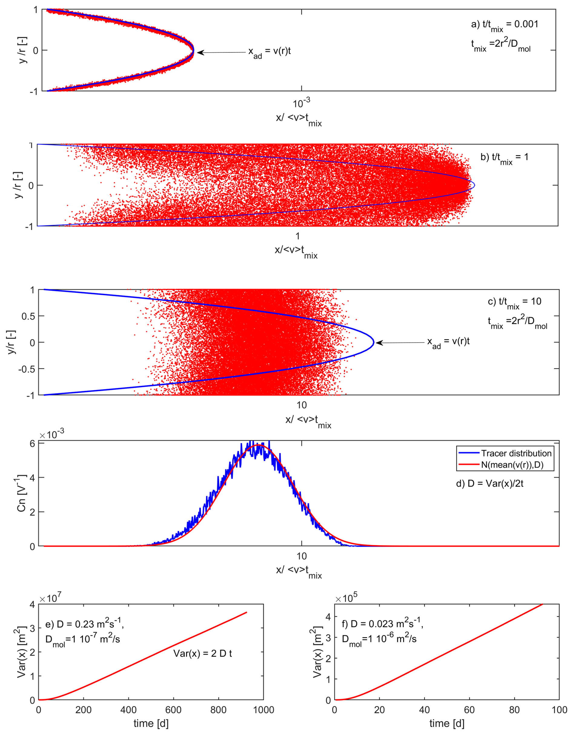
Figure 1 The three stages of Taylor-Aris dispersion in a capillary tube pore with radius r (m) as a function of the diffusive mixing time scale $t_{\mathrm{mix}}=\mathrm{2}r/D_{\mathrm{mol}}$: (a) near field for t≪t_mix, intermediate state for t=t_mix (b) and well mixed far field for t≫t_mix (c). Variance of particle transport distances as a function of time for $D_{\mathrm{mol}}=\mathrm{1}\times {\mathrm{10}}^{-\mathrm{6}}$ m² s⁻¹ (e) and $D_{\mathrm{mol}}=\mathrm{1}\times {\mathrm{10}}^{-\mathrm{7}}$ m² s⁻¹ (f). All graphs were inferred from transport simulations based on particle tracking.

The comparison of the travel distance distribution inferred from the particles to the Gaussian distribution in Fig. 1c corroborates that indeed a Gaussian travel time distribution emerges. The mean travel distance grows with the spatially averaged fluid velocity, $\stackrel{\mathrm{‾}}{v}$, and t (Fig. 1d). The variance of travel times now grows linearly with t and the slope is the macro-dispersion coefficient D (Fig. 1e, f). For Taylor-Aris dispersion in a cylindrical pore with radius r, the dispersion coefficient shows the following dependency:

$$\begin{array}{}\text{(3)}& D\sim {\displaystyle \frac{{\stackrel{\mathrm{‾}}{v}}^{\mathrm{2}}{r}^{\mathrm{2}}}{D_{\mathrm{mol}}}}.\end{array}$$

The key point is that D grows linearly with $D_{\mathrm{mol}}^{-\mathrm{1}}$. Figure 1 corroborates for the simulated transport of two different tracers with D_mol of $\mathrm{1}\times {\mathrm{10}}^{-\mathrm{7}}$ (Fig. 1e) and $\mathrm{1}\times {\mathrm{10}}^{-\mathrm{6}}$ m² s⁻¹ (Fig. 1f). Diffusion that is slower by a factor of 10 causes not only a ten times larger dispersion coefficient: it also implies that it takes ten times longer to reach the well-mixed advective-dispersive case and that the variance in travel distances increases ten times faster with time.

Of course, we acknowledge that dispersion in a real-world porous medium relates to the variability in pore sizes and that the geometry and tortuosity of soil pores is clearly more complex than the above example. Naturally, this implies that dispersion in a porous medium shows a qualitatively different behavior. In one dimension, the dispersion coefficient is proportional to the product of the average flow velocity, $\stackrel{\mathrm{‾}}{v}$, (not ${\stackrel{\mathrm{‾}}{v}}^{\mathrm{2}}$), and the dispersivity of the porous medium. The latter characterizes the length scale of heterogeneities (Bear, 1972; Dentz et al., 2023). Yet we argue that Taylor dispersion and Hagen-Poiseuille flow occur in each individual soil pore. This implies the lateral diffusive mixing times for isotopic tracers will be different due to their different diffusion coefficients, meaning that we expect the tracer with lower diffusion coefficient will experience a stronger longitudinal dispersion. We thus conjecture that the variance of travel distances and travel times will, nevertheless, grow with a decreasing molecular diffusion coefficient. However in the case of perfect mixing, we do not expect that different isotopes will show different mean travel times, simply because advective-dispersion transport relies on a linear superposition of advective and dispersive solute flux, and the average flow velocity $\stackrel{\mathrm{‾}}{\mathit{v}}$ is not affected by changes in the diffusion coefficient.

$$\begin{array}{}\text{(4)}& \mathit{j}=\stackrel{\mathrm{advective}\mathrm{solute}\mathrm{flux}}{\overbrace{\mathit{v}C}}-\stackrel{\mathrm{dispersive}\mathrm{solute}\mathrm{flux}}{\overbrace{D\mathrm{\nabla }C}}.\end{array}$$

Instead, we propose that the independence of the average transit time from the diffusion coefficient no longer holds when non-Fickian transport occurs. The latter breaks the symmetry of the Gaussian travel distance distribution (Bloschl and Zehe, 2005), because molecules are either trapped in low conductive bottlenecks for very long times, and/or are traveling along rapid preferential flow paths leaving the system after very short times (Berkowitz and Zehe, 2020; Wienhöfer et al., 2009). As an important implication of the long tailing, the travel time distribution becomes skewed and in the case of advective trapping in low conductive bottlenecks, one might expect that an isotope with a smaller diffusion coefficient stays in the bottlenecks for longer times compared to an isotope which exhibits faster diffusion. This could imply that in case of non-Fickian transport average transit times grow with a decreasing diffusion coefficient.

2.2 Transport simulations and numerical experiments

To shed light on the role of the different diffusion coefficients of deuterium, tritium and O¹⁸ for the transit time distributions, we simulated advective-diffusive transport through steady-state flow fields in two dimensional saturated domains of increasing heterogeneity, comparing the transport of the three different water isotopes. Their respective diffusion coefficients in water at a temperature of 25 °C are, according to Devel (1962) and Wang et al. (1952), $D_{\mathrm{HDO}}=\mathrm{2.25}\times {\mathrm{10}}^{-\mathrm{9}}$ m² s⁻¹, $D_{\mathrm{HTO}}=\mathrm{2.44}\times {\mathrm{10}}^{-\mathrm{9}}$ m² s⁻¹ and $D_{{}^{\mathrm{18}}{\mathrm{OH}}_{\mathrm{2}}}=\mathrm{2.66}\times {\mathrm{10}}^{-\mathrm{9}}$ m² s⁻¹. For the case of HTO we chose to ignore its radioactive decay, to assure that optional differences in average travel times stem only from the differences in diffusion coefficients.

In all investigated cases we used particle tracking to simulate isotope transport in combination with the respective flow fields. The particle advancement, Δs (m), being characterized by the Langevin equation, starting from a given particle location at time t_i:

$$\begin{array}{}\text{(5)}& \mathrm{\Delta }s(x,y)=\mathit{v}\left[\mathit{s}\left(t_i\right)\right]\mathrm{\Delta }t+\mathit{\xi }\sqrt{\mathrm{2}{D}_{\mathrm{mol}}\mathrm{\Delta }t}\end{array}$$

The first term characterizes advective displacement, depending on the two dimensional (2d) fluid velocity vector v, and the time step Δt. The second term denotes the diffusive displacement, which scales with a modulus of $\sqrt{\mathrm{2}{D}_{\mathrm{mol}}\mathrm{\Delta }t}$ times a standard normally distributed random number ξ.

Three different model scenarios, A, B, and C, are examined, accounting for different types of hydraulic conductivity fields and heterogeneities. In all cases tested, the dependence of the simulations on the chosen number of particles compared N=10⁴, 5×10⁴, 10⁵ and 2×10⁵; results were independent of N at particle numbers larger than 10⁵. In all cases fluid velocities were interpolated to the particle position using inverse distance weighting.

2.2.1 Scenario A: Isotope transport through a homogeneous medium with an embedded lower permeable lens

Scenario A was inspired by the experimental work of Elhanati et al. (2025) investigating the breakthrough of deuterium and Br⁻ through homogeneous, uniformly packed sand columns and sand columns with an embedded lower permeable lens (Fig. 2, Scenario A). We simulated steady flow through a 1 m by 10 m block using the following configurations:

•  

  A1.1 – a sandy saturated soil with hydraulic conductivity $K_{\mathrm{s}}=\mathrm{1}\times {\mathrm{10}}^{-\mathrm{5}}$ m s⁻¹ and porosity of 0.4, surrounding a less conductive lens (Fig. 2) with hydraulic conductivity of $K_{\mathrm{s}}={\mathrm{10}}^{-\mathrm{9}}$ m s⁻¹.

•  

  A.1.2 – same configuration as A1.1, while the less conductive lens has a hydraulic conductivity of $K_{\mathrm{s}}={\mathrm{10}}^{-\mathrm{8}}$ m s⁻¹

•  

  A2.1 – a saturated loess soil with hydraulic conductivity $K_{\mathrm{s}}=\mathrm{1}\times {\mathrm{10}}^{-\mathrm{7}}$ m and porosity of 0.46, surrounding a less conductive lens (Fig. 2) with hydraulic conductivity of $K_{\mathrm{s}}={\mathrm{10}}^{-\mathrm{9}}$ m s⁻¹.

•  

  A2.2 – same configuration as A2.1, while the less conductive lens has a hydraulic conductivity of $K_{\mathrm{s}}={\mathrm{10}}^{-\mathrm{8}}$ m s⁻¹.

In all cases, we used a discretization of 0.2 m by 0.2 m, a permeameter type of boundary condition with a head gradient of 0.05 m m⁻¹, and calculated the flow field using the model CATLFOW (Zehe et al., 2001). CATFLOW is a physically based model to simulate the water balance and subsurface transport at hillslope scale. CATFLOW simulates subsurface water dynamics based on the two dimensional Darcy-Richards equation using curvilinear orthogonal coordinates. The equation is solved using a mass conservative Picard iteration (Celia et al., 1990) with adaptive time stepping. While the model also accounts for overland flow, evaporation and transpiration and solute transport, we omit details here as we make use solely of the simulated steady state flow fields. The flow fields were generated using no-flow boundary conditions on the horizontal domain boundaries. Using these flow fields, we simulated advective diffusive transport by means of particle tracking according to Eq. (5) and time steps of 1 h and 10⁵ particles. As scenario A is partly an upscaled version of the medium that Elhanati et al. (2025) used in their experiments, we expect that non-Fickian transport will emerge in line with their experimental findings. However, it was not possible to reconstruct the exact hydraulic conductivities of these experiments, so that we expect similar qualitative behavior but not a one-to-one correspondence.

Figure 2 Scheme of model scenarios.

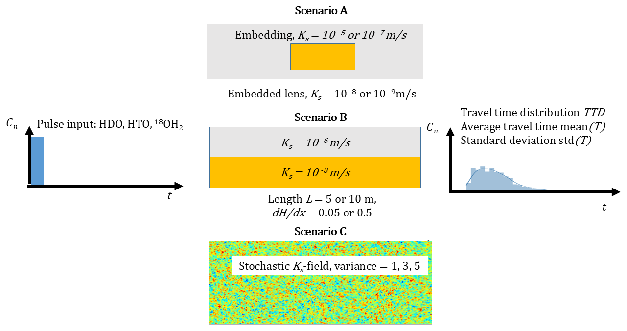
2.2.2 Scenario B: Isotope transport through a two-layered aquifer at different head gradients

In scenario B, we simulated advective-diffusive solute transport in a simple two-layer aquifer system of 2 m total height and a length of either 10 m (B1) or 5 m (B2). The layers with a height of 1 m are homogeneous but differ by their saturated hydraulic conductivity of $K_{\mathrm{s}}={\mathrm{10}}^{-\mathrm{6}}$ and 10⁻⁸ m s⁻¹. Both layers were exposed to the same head gradient, which was first set to $\mathrm{d}H/\mathrm{d}x=\mathrm{0.05}$ and then to $\mathrm{d}H/\mathrm{d}x=\mathrm{0.5}$ to compare overall four different Peclet numbers. Transport of deuterium, tritium and ¹⁸O with their diffusion coefficients was simulated using a pulse input of 10⁵ particles through the left upstream domain, while no-flow conditions were assigned to the two horizontal domain boundaries. Time stepping was set to one hour.

2.2.3 Scenario C: Isotope transport through a stochastic heterogeneous aquifer with increasing variance in hydraulic conductivity

In scenario C (Fig. 2, Scenario C; Fig. 3), we revisited steady-state fluid flow within two-dimensional, stochastic heterogeneous media with moderate (var = 1), intermediate (var = 3) and strong variance (var = 5) in the hydraulic conductivity from the study of Zehe et al. (2021). The 60 m long and 20 m wide domain was discretized into 0.2 m by 0.2 m elements. Flow was driven by total difference ΔH=10 m, from the left upstream boundary to the right downstream boundary, while no-flow conditions were assigned to the two horizontal domain boundaries. We used random and yet statistically homogeneous, isotropic Gaussian fields of three different variance of ln (K), namely 1, 3 and 5 generated with the sequential Gaussian simulator GCOSIM3D (Gómez-Hernández et al., 1997) and a correlation length of 1 m. Advective diffusive transport was again simulated using particle tracking according to Eq. (5).

Our previous work showed that these media were highly susceptible to preferential flow and transport, while one could observe a stronger funneling into preferential flow paths with increasing variance (Edery et al., 2014; Zehe et al., 2021), as visualized in Fig. 3. For the particle tracking we used simulated flow fields for an average hydraulic conductivity of $K_{\mathrm{s}}={\mathrm{10}}^{-\mathrm{7}}$ m s⁻¹ or $K_{\mathrm{s}}={\mathrm{10}}^{-\mathrm{6}}$ m s⁻¹ to account for two different Peclet numbers, injecting 10⁵ particles at the upstream left boundary and using hourly time steps.

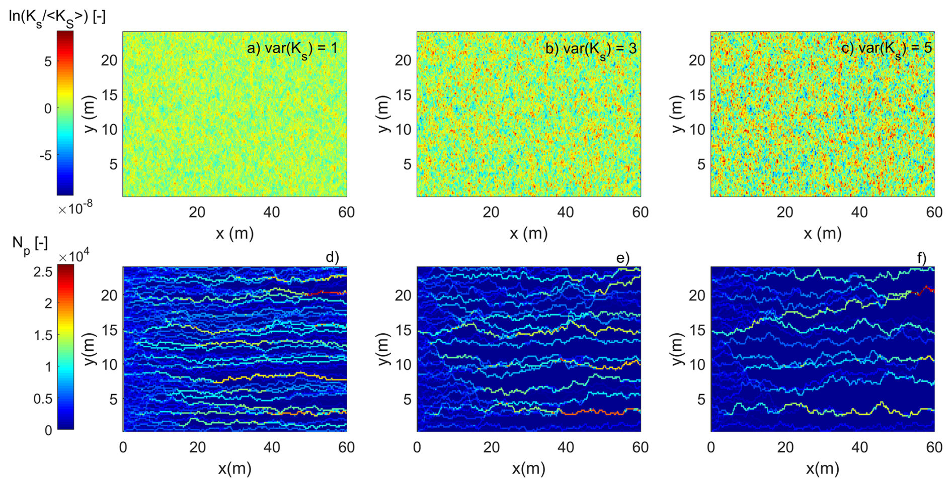
Figure 3 The normalized hydraulic conductivity fields for three randomly selected realizations of small, medium and large variance (a, b, c). Normalized cumulative number of particles (Np) that visited a grid cell in the simulation domain for small, medium and large variance (d, e, f) for HDO inferred from a critical flow path analysis. Funneling of water and HDO into preferred pathways become clearer stronger with increasing variance of the hydraulic conductivity field.

3 Results

3.1 Travel time distributions inferred from scenario A

While scenario A did not generally yield distinct differences in the simulated travel time distribution for different isotopic tracers, we found for all scenarios travel time distributions with longer tails. Figure 4 shows this exemplarily for scenarios A2.1 and A2.2 (the conductive embedding) by comparing their travel time distributions, derived from the accumulated normalized breakthrough curves (CBTC), using the transport through the homogeneous medium without a clay lens as a well mixed, Gaussian reference. This reveals, in line with the experimental evidence of Elhanati et al. (2025), a clearly non-Fickian travel time distribution with an earlier first arrival and significantly longer tailing compared to the Gaussian reference (black line, Fig. 4). In addition, Table 1 provides the mean travel time (mean(T)), its standard deviation (SD(T)), as well as the 10 %, 20 % 50 %, 75 % and 90 % quantiles (T10, T25, T50, T75, T90). Case 2.1 (solid green) has clearly the smallest average travel time, due to the faster first arrival, while it has also a larger standard deviation and a longer tailing, compared to the Gaussian case. So here the earlier first arrival dominates against the longer tail. Mean travel times drop below that of the Gaussian reference when the hydraulic conductivity of the clay lens is increased from 10⁻⁹ to 10⁻⁸ m s⁻¹ (Fig. 4, solid red A.2.2), despite the earlier first arrival. This can be explained by a stronger advective transport of the tracer into the lens, due to the smaller drop in conductivity. This clearly leads to a much longer tailing, which ultimately controls the shift to larger mean travel times. Consistently, we observe an even larger mean travel time, when elongating the clay lens with $K_{\mathrm{s}}={\mathrm{10}}^{-\mathrm{8}}$ m s⁻¹ by 30 % (Fig. 4. A.2.2 long, solid blue).

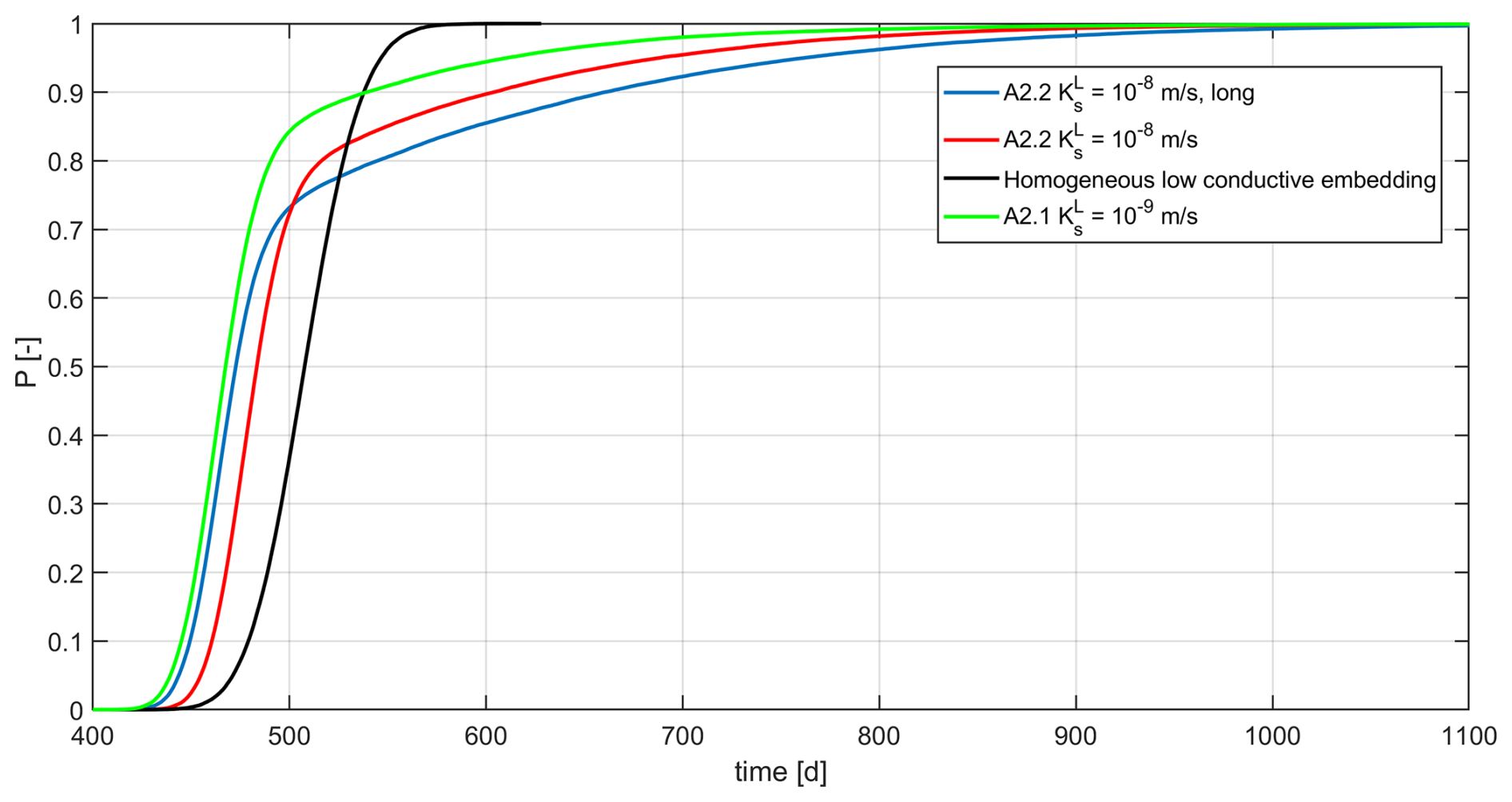
Figure 4 Cumulative breakthrough curves/travel time distributions of HDO for scenario A.2.1 and A. 2.2, i.e., the low conductive embedding medium with $K_{\mathrm{s}}={\mathrm{10}}^{-\mathrm{7}}$ m s⁻¹, using the travel time distribution through the homogeneous medium as reference.

Table 1 Mean travel time (mean(T)), standard deviation (SD(T)), as well as the 10 %, 20 % 50 %, 75 % and 90 % quantiles (T10, T25, T50, T75, T90) for cases shown in Fig. 4. For convenience we includehe hydraulic retention time, RT_hyd.

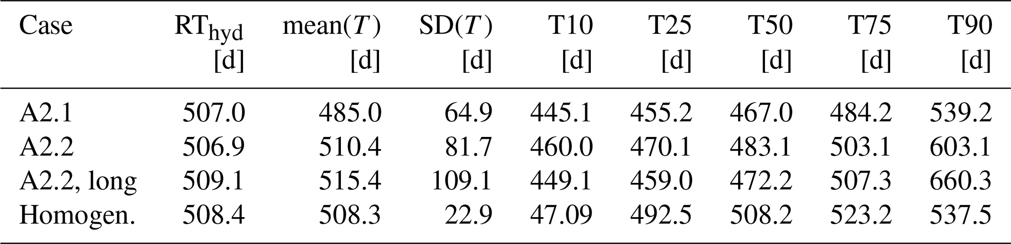
For convenience, we compared the mean travel time, mean(T), to the average hydraulic retention time, RT_hyd, calculating the latter by dividing the total pore volume of the domain by the averaged flow rate. RT_hyd and mean(T) match naturally very well for the case of Fickian transport through the homogeneous domain. In the case of non-Fickian transport, however, we observe that the average travel times inferred from the CBTCs deviate from the hydraulic retention time RT_hyd. In case 2.1 it is actually smaller while in case 2.2 it is slightly larger.

We generally acknowledge that one can a priori expect deviations from Fickian transport in scenario A, as the transport distance is only twice as large as the length of the embedded clay lens. Yet, the long tail reflects diffusion of molecules into the low conductive lens, which evidently reside there for considerably long times. The channeling of the flow around the lens and the enlarged transport velocities explain in turn the earlier arrival of the solutes compared to the homogeneous case.

3.2 Travel time distributions inferred from scenario B

Figure 5 provides the cumulative breakthrough curves/travel time distributions (TTD) through the two layered system of 10 m (B1) and 5 m length (B2) at the two different head gradients. In all cases we found a distinct dependence of the TTD on the diffusion coefficient of the different isotopes. Generally, HDO exhibits in all cases the largest mean travel time followed by HTO followed by ¹⁸OH₂ (Table 2). A slower diffusion implies indeed a shift towards longer travel times, which manifest particularly in the long tails and the larger quantiles (Table 2). To highlight these differences, Fig. 5 zooms to travel times larger than the 80 % quantiles and smaller than 99 % quantiles. We found however also that the standard deviation and thus the dispersion of travel times grows systematically with declining diffusion coefficient.

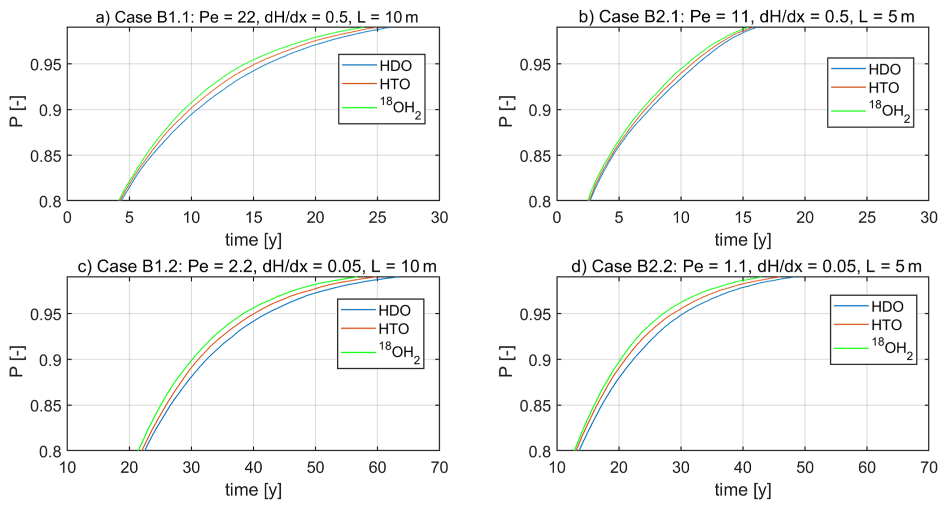
Figure 5 Travel time distributions of HDO (solid green), HTO (solid red) and ¹⁸OH₂ (solid blue) for the long aquifer (B1, a and c) the short layered aquifer (B2, c and d), with the driving head gradient $\mathrm{d}H/\mathrm{d}x$ and the corresponding Peclet numbers. For a better visualization of the main differences, we zoom to travel times larger than the 80 % and lower than the 99 % quantiles. Note that scaling of the ordinate in (a) and (b), as well as (c) and (d) are different.

Table 2 Mean travel time (mean(T)), standard deviation (SD(T)), as well as the 10 %, 20 % 50 %, 75 % and 90 % quantiles (T10, T25, T50, T75, T90) for cases shown in Fig. 5. The color coding corresponds to the plots of the different isotopes in Fig. 5.

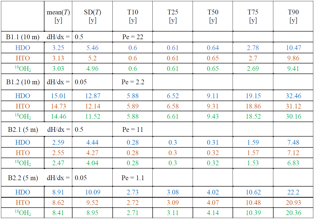
The median travel times in Table 2 grow for both large head gradients almost linearly with transport distance, from approx. 4 to 9 years (for the small gradient) 0.32 to approx. 0.65 years (for the large gradient). However, for each travel distance, driving head and isotope the mean travel time is minimum two and maximum five times larger than the corresponding median, which underlines that TTD are strongly skewed due to very long tails. Absolute differences between mean travel times are largest comparing HDO and ¹⁸OH₂. They appear largely independent from the length of the aquifer ranging from approx. 0.2 years for the larger head gradient to approx. 0.5 years for the small gradient. The corresponding relative differences decline naturally with increasing length of the aquifer ranging from 7 % to 4 %. Interestingly, we can observe a rather stable relative difference between the standard deviation of travel times of HDO and ¹⁸OH₂ of approximately 10 %, which implies that differences in their variance and thus dispersion are approximately 20 %. This relative difference corresponds well to the relative difference between the diffusion coefficients of $D_{\mathrm{HDO}}=\mathrm{2.25}\times {\mathrm{10}}^{-\mathrm{9}}$ m² s⁻¹ and $D_{{}^{\mathrm{18}}{\mathrm{OH}}_{\mathrm{2}}}=\mathrm{2.66}\times {\mathrm{10}}^{-\mathrm{9}}$ m² s⁻¹.

3.3 Travel time distributions inferred from scenario C

Figure 6 presents the travel time distributions for scenario C for all isotopic tracers, variance in hydraulic conductivity grows from the top to the bottom rows, cases with mean(K_s) = $\mathrm{1}\times {\mathrm{10}}^{-\mathrm{6}}$ m s⁻¹ appear in the left column, those with mean(K_s) = $\mathrm{1}\times {\mathrm{10}}^{-\mathrm{7}}$ m s⁻¹ appear in the right column. In all cases except C1.1, there is a distinct dependence of the TTD on the diffusion coefficient. Generally, HDO exhibits the largest mean travel time followed by HTO followed by ¹⁸OH₂ (Table 3). The TTD of C.1.1 (var = 1, mean(K_s) = $\mathrm{1}\times {\mathrm{10}}^{-\mathrm{6}}$) is very close to the well mixed case, as the mean and median travel times are for all isotopes very similar. Differences in mean and median travels generally grow when moving to larger variances, while differences in travel time distributions become more distinct particularly in the 75 % and 90 % quantiles (Table 3) and the tails (Fig. 6).

Table 3 Mean travel time (mean(T)), standard deviation (SD(T)), as well as the 10 %, 20 % 50 %, 75 % and 90 % quantiles (T10, T25, T50, T75, T90) for cases shown in Fig. 6. The color coding corresponds to the plots of the different isotopes in Fig. 6.

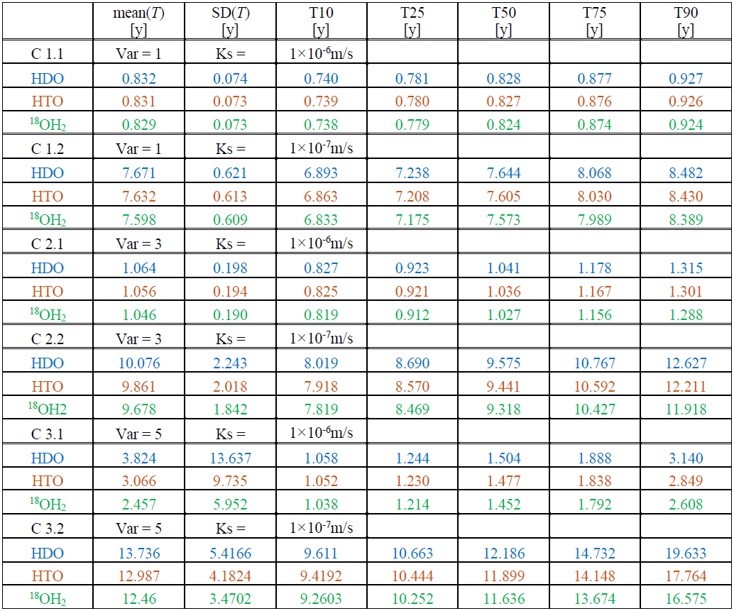
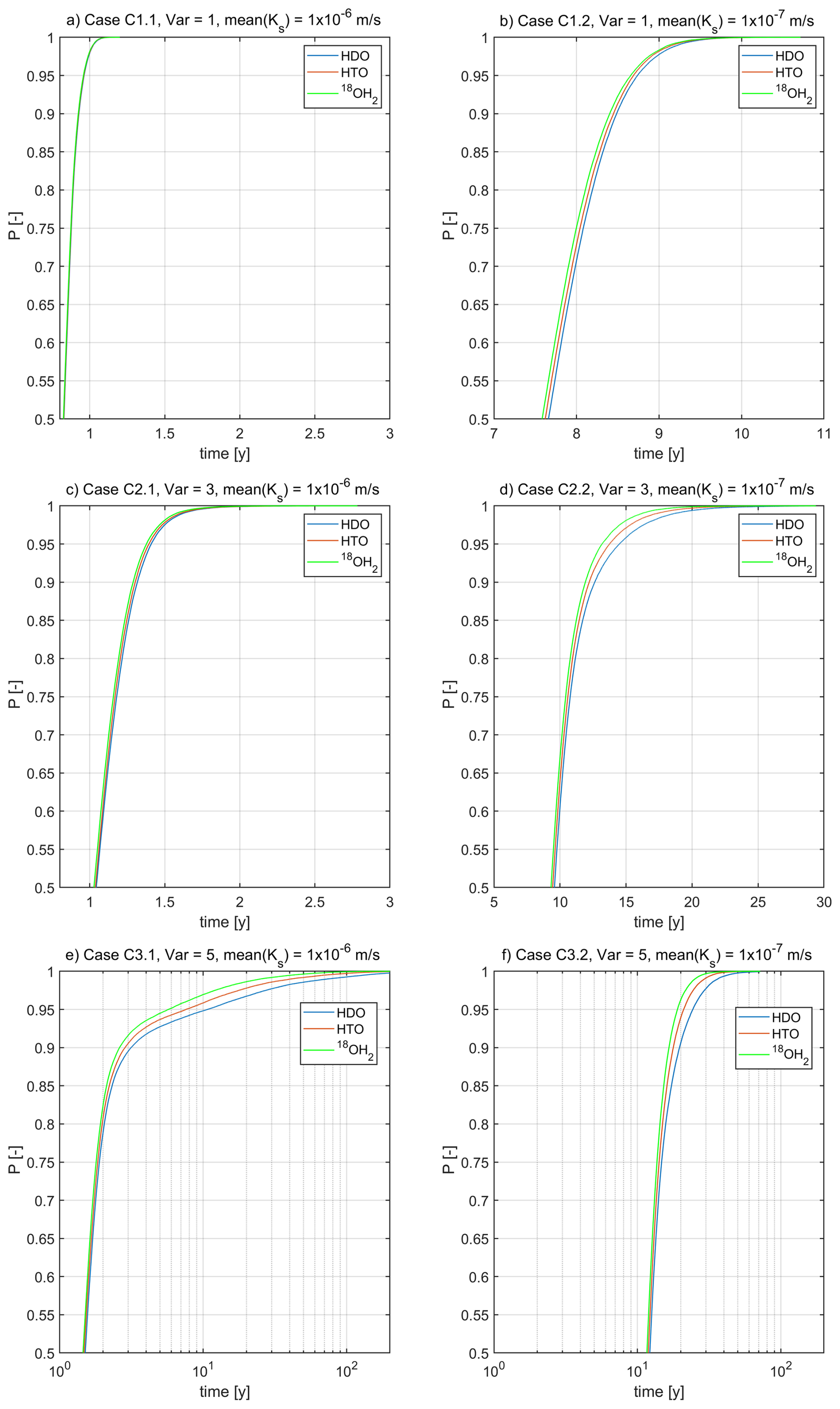
Figure 6 Travel time distributions of HDO (solid green), HTO (solid red) and ¹⁸OH₂ (solid blue) for scenario C; variance in hydraulic conductivity grows from the top to the bottom rows, cases with mean(K_s) = $\mathrm{1}\times {\mathrm{10}}^{-\mathrm{6}}$ m s⁻¹ appear in left column, those with mean(K_s) = $\mathrm{1}\times {\mathrm{10}}^{-\mathrm{7}}$ m s⁻¹ appear in the right column. For a better visualization of the main differences, we zoom to travel times larger than the median. Note that scaling of the ordinates is different, color coding is consistent with Table 3.

Significant absolute differences in the mean travel times of HDO and ¹⁸OH₂ occur for C2.2 (var = 3, lower K_s) with approximately 0.4 years, and particularly for both cases with variance of 5 (C3.1 and C.3.2) with absolute difference of approximately 1.4 years. The case of the lower mean hydraulic conductivity corresponds to a relative difference of 10 %. For the higher mean hydraulic conductivity we observe, however, that HDO (mean(T) = 3.83 years) travels on average 50 % slower than ¹⁸OH₂ (mean(T) = 2.46 years). The reason for this high relative difference is that the 10 times higher conductivity leads to earlier first arrival while the travel times still exhibit very long tailing with substantial differences between the isotopes. Note that for C3.1 differences in the mean travel time of HDO (mean(T) = 3.83 years) and HTO (mean(T) = 3.1 years) are with approximately 0.75 years, substantially larger than the differences reported by Rodriguez et al. (2021) for the respective median travel times. To summarize, we argue that standard deviations of travel times are distinct among the isotopes, particularly when considering larger variances in hydraulic conductivities. Maximum relative differences amount to 20 % between HDO and HTO as well as HTO and ¹⁸OH₂ (C3.1 and C3.2), which implies that the dispersion will vary by approximately 40 %.

4 Discussion and conclusions

Our study provides clear evidence that the sensitivity of travel time distributions to small changes in diffusion coefficients is – albeit partly relatively small – not a question of measurement error but a question of transport physics. Differences generally manifest as differences in higher quantiles and thus in the tailing behavior, as well as for the mean travel times and standard deviations. Particularly, for the case of strongly heterogeneous, stochastic media and anomalous transport, we demonstrate that differences in average travel times of different water isotopes (HDO, ¹⁸OH², HDO) can deviate by as much as 1.3 years, which corresponds to relative differences of 10 % and a maximum 50 %. We found the strongest relative differences of the order of 50 % for stochastic heterogeneous medium with a variance of 5 in the log hydraulic conductivity and a mean value of K_s = $\mathrm{1}\times {\mathrm{10}}^{-\mathrm{6}}$ m s⁻¹. We found smaller differences of the order of 3 % to 7 % for simple two layered media. Given their size, one could be inclined to erroneously interpret these differences as measurement errors. However, these differences are indeed physical and reflect tracers with smaller diffusion coefficients that eventually remain over longer times in low conductive bottlenecks, which enlarges the tails and average travel times. Thus, these effects do not average out, but persist when doubling the transport distances.

Furthermore, we found that in the case of simple layered systems and in heterogeneous stochastic environments, the standard deviation and thus the dispersion of the travel times grow distinctly with declining diffusion coefficients, with a relative difference of up to 20 %. This is qualitatively the same behavior as what is known from Taylor-Aris dispersion and confirms our related hypothesis.

Our findings are in line with the experiments of Elhanati et al. (2025) and corroborate that water isotopes show similar behaviors to Br⁻. The molecular diffusion coefficient of bromide is $\mathrm{2.01}\times {\mathrm{10}}^{-\mathrm{9}}$ m² s⁻¹, indeed close to that of HDO ($\mathrm{2.22}\times {\mathrm{10}}^{-\mathrm{9}}$ m² s⁻¹). Our study corroborates furthermore the argument of Stewart et al. (2010, 2021), namely that averaged travel times inferred from ¹⁸O might in the case of two-layered mobile and immobile storage regions, or of a strongly heterogeneous subsurface, be systematically shorter than those inferred from tritium. The maximum differences we found are 0.6 years, which correspond to a relative difference of approximately 30 %. The latter corresponds to the difference Stewart et al. (2010) reported for the Brugga catchment, which has an average travel time of order 3–6 years for deep groundwater. Stewart et al. (2010) reported an even larger difference between mean($T_{{}^{\mathrm{18}}{\mathrm{OH}}_{\mathrm{2}}}$) = 3.4 years to mean(T_THO) = 9.6 years for the Pukemanga catchment. We cannot expect to detect similarly large differences here, because we did not account for radioactive decay of tritium (half-life of 12.32 years). Based on this decay one might detect contributions of rather old water, that typically cannot be resolved based on differences in ¹⁸O. At this stage we return to the comprehensive demonstration of Wang et al. (2023), who found broadly equivalent magnitudes of water ages inferred from ³H and ¹⁸O when using the SAS approach, but substantial differences when using a transfer function approach. One could thus be inclined to attribute at least some of the difference to the use of the transfer function. However, in this context it is also important to note that Rodriguez et al. (2021) found relative differences of approximately 0.23 % in mean water ages in the Weiherbach using the SAS approach and even larger differences as corroborated in this study.

We thus conclude that travel time distributions of isotopic tracers reflect the spectrum of fluid velocities and diffusive/dispersive mixing between the flow lines connecting inputs and outputs to the system. Travel time distributions of isotopic tracers might thus reflect the differences in their diffusion coefficients, which are of order 10 %, and in the case of non-Fickian transport this eventually also affects substantially the mean travel time, its variance, and in particular, travel times larger than the 80 % quantile.