Streamflow elasticity as a function of aridity

Relating variations in annual streamflow to a climate anomaly, commonly referred to as streamflow elasticity to climate, is central for a rapid assessment of the impact of climate change on water resources. This elasticity is classically estimated via a multiple linear regression between anomalies in streamflow and climate variables. However, this approach does not explicitly account for the fact that elasticity depends on aridity as suggested by “Budyko-type” water balance formulas. Using a large dataset of 4122 catchments from four continents, we first verify empirically the link between elasticity and aridity. Then, we propose a method to constrain elasticity coefficients with derivatives from a “Budyko-type” water balance formula, that allows introducing an explicit dependency between elasticity and aridity. We show that adding this dependency produces a regionalized elasticity formula with physically-realistic elasticity coefficients.

1 Introduction

1.1 About streamflow elasticity

The climate elasticity of streamflow (Schaake and Liu, 1989; Dooge et al., 1999; Sankarasubramanian et al., 2001) describes the sensitivity of streamflow to changes in a climate variable. Elasticity is classically derived from the following regression:

$$\begin{array}{}\text{(1)}& \mathrm{\Delta }{Q}_n=e_{Q/P}\mathrm{\Delta }{P}_n+e_{Q/E_{\mathrm{0}}}\mathrm{\Delta }{E}_{\mathrm{0}n}\end{array}$$

where: $e_{Q/P}$ denotes the precipitation elasticity of streamflow, $e_{Q/E_{\mathrm{0}}}$ denotes the potential evaporation elasticity of streamflow; both coefficients are dimensionless. Note that elasticity is defined here in absolute terms, i.e. as the sensitivity between quantities of the same dimension (ΔQ, ΔP and ΔE₀ are all in mm yr⁻¹) following Andréassian et al. (2016).

Andréassian et al. (2025) recently proposed to enrich the traditional computation given in Eq. (1), to account for the seasonal time shift between precipitation and potential evaporation, because of its decisive impact on catchment water yield (see e.g. Pardé, 1933; Coutagne and de Martonne, 1934; Thornthwaite, 1948; Milly, 1994; Yokoo et al., 2008; Roderick and Farquhar, 2011; de Lavenne and Andréassian, 2018; Feng et al., 2019). We compute the synchronous amount of precipitation and potential evaporation Λ, using monthly data as in Eq. (2):

$$\begin{array}{}\text{(2)}& {\mathrm{\Lambda }}_n={\displaystyle \frac{{\sum }_{m=\mathrm{1}}^{\mathrm{12}}min(P_{m,n},E_{{\mathrm{0}}_{m,n}})}{\sqrt{P_n\cdot E_{{\mathrm{0}}_n}}}}\cdot \stackrel{\mathrm{‾}}{P}\end{array}$$

Where index m stands for the month. The dimension of Λ_n is mm yr⁻¹ and it represents the annual precipitation volume most easily accessible to evaporation. For two years with the same annual amounts of precipitation and potential evaporation, Λ will be higher when they are synchronous, and lower when they are out of phase (for more details, please refer to Andréassian et al., 2025). With this new term, the regression in Eq. (1) becomes:

$$\begin{array}{}\text{(3)}& \mathrm{\Delta }{Q}_n=e_{Q/P}\mathrm{\Delta }{P}_n+e_{Q/E_{\mathrm{0}}}\mathrm{\Delta }{E}_{\mathrm{0}n}+e_{Q/\mathrm{\Lambda }}\mathrm{\Delta }{\mathrm{\Lambda }}_n\end{array}$$

1.2 Using aridity to estimate streamflow elasticity

The link between streamflow elasticity and catchment aridity is a well-established concept in hydrology, an idea that can be traced back to Oldekop (1911) and his followers, including Budyko (1948), Bagrov (1953) and Mezentsev (1955). Many “modern” hydrologists such as Dooge (1992) and Dooge et al. (1999) discussed the form that aridity-dependent streamflow formulas could take. This dependency was emphasized by Koster and Suarez (1999), who write that “the partitioning of a precipitation anomaly into evaporation and runoff anomalies is a simple function of the dryness index”, as well as by Sankarasubramanian et al. (2001) who argue that empirical elasticity estimates would only follow the direction shown by the Budyko-type formulas for the very humid regions of the US, while Arora (2002) concludes that “the use of aridity index provides a straight-forward method to obtain a first order estimate of the effect of climate change on annual runoff”. Chiew (2006) shows the dependency of streamflow elasticity on aridity, Renner et al. (2012) stress that the elasticity of streamflow “is largely dependent on […] the aridity of the climate” and Roderick and Farquhar (2011) underline that “the response of runoff to changes in the main driving variables is not constant but depends on the overall climatic dryness”.

More recently, the concept has been applied at a global scale, with Berghuijs et al. (2017) who use the elasticity pattern provided by the Tixeront-Fu formula to propose a world map of aridity-dependent streamflow elasticities, Zhang et al. (2022) discuss the impact of aridity on the sensitivity of the elasticity coefficient to the aggregation time step, and Anderson et al. (2024) extends the computation of elasticity to different flow quantiles, and show that aridity impacts the shape of the curve relating the different elasticity quantiles.

However, Addor et al. (2018), using random forests to explain (among others) the precipitation elasticity of streamflow, concluded that signatures of “hydrological dynamics are poorly predicted by aridity alone, or even by a combination of several climatic indices”.

1.3 Local vs. class estimation of elasticity

To estimate the climate elasticity of streamflow at regional or national scales, making the dependency of streamflow elasticity on aridity explicit can constrain the estimation of elasticity coefficients and increase their physical realism.

For a given catchment with a sufficiently long series of annual observations, streamflow elasticity can be computed locally by linear regression (Andréassian et al., 2016). However, for ungauged catchments, local estimation of elasticity coefficients is no longer possible. Instead, a class-elasticity can be estimated by combining all available records in a region. The estimation by class has both advantages and drawbacks. While this approach improves the statistical significance of elasticity coefficients, which can have high uncertainty when estimated locally (especially for potential evaporation), it also requires combining data from catchments with different aridity indices. This presents a challenge, precisely because we know that aridity and elasticity are linked.

Methods to estimate local- and class-elasticity are detailed in Sect. 2.

1.4 Formulas relating streamflow elasticity to aridity

We mentioned above the seminal work of the hydrologists who, following Oldekop (1911), developed various mathematical formulas to represent catchment water balance. These studies established simple water balance formulas from which a “theoretical” elasticity of streamflow can be derived as their partial derivatives. In Table 1, we present four long-term water balance formulas that can be used to provide these theoretical elasticity estimates. The Schreiber and Oldekop formulas are parameter-free, while the Turc–Mezentsev and Tixeront-Fu formulas each have one parameter (ω¹ and m, respectively). These last two formulas are equivalent when setting $m=\mathit{\omega }+\mathrm{0.72}$ (Yang et al., 2008; Andréassian and Sari, 2019), which explains why their curves overlap in some of the later figures.

Table 1 Common long-term water balance formulas and the associated elasticities ($\stackrel{\mathrm{‾}}{Q}$ – long-term average streamflow [mm yr⁻¹], $\stackrel{\mathrm{‾}}{P}$ – long-term average precipitation [mm yr⁻¹], $\stackrel{\mathrm{‾}}{E_{\mathrm{0}}}$ – long-term average reference evaporation [mm yr⁻¹], $\mathit{\phi }=\frac{\stackrel{\mathrm{‾}}{E_{\mathrm{0}}}}{\stackrel{\mathrm{‾}}{P}}$ is the aridity index).

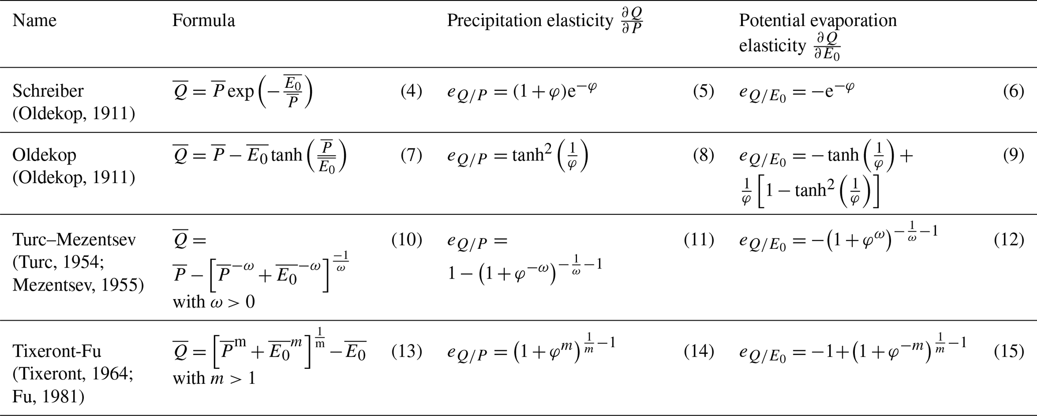
Table 1 also presents the partial derivatives for each formula, allowing to compute the precipitation and the potential evaporation elasticities of streamflow. Unsurprisingly, these formulas are all functions of the aridity index.

Figure 1 illustrates the similarities and differences among the formulas by showing their respective elasticity-aridity relationships. The embedded dependency on aridity is clearly visible, and we notice that the four formulas have distinct but similar shapes (with the difference between the Turc–Mezentsev and the Tixeront-Fu being negligible). Furthermore, the precipitation elasticity is bounded between 0 and 1, which means that one millimeter of additional precipitation will always result in less than one millimeter of additional streamflow. Similarly, the potential evaporation elasticity is bounded between 0 and −1, which means that one millimeter of additional potential evaporation will always result in a decrease of streamflow of less than one millimeter. These bounds represent a physically-realistic catchment response, in the sense that the yield (of the additional mm of precipitation or the additional mm of potential evaporation) must be comprised (in absolute value) between 0 % and 100 %.

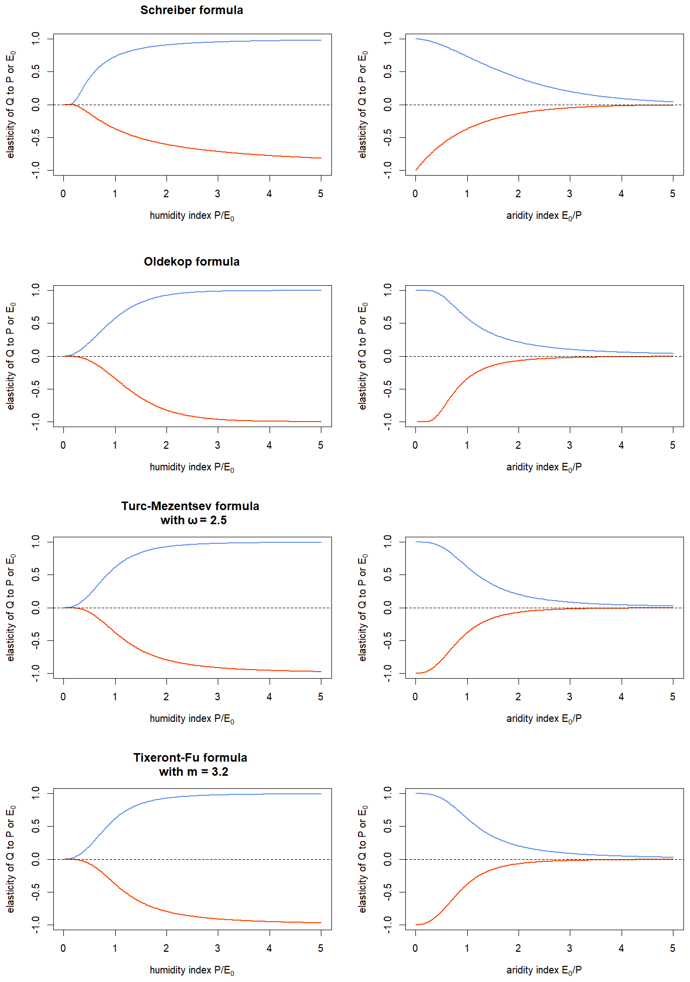
Figure 1 Theoretical relationships between streamflow elasticities and the humidity index (left panel) and the aridity index (right panel). Blue lines represent the precipitation elasticity of streamflow, and orange lines represent the potential evaporation elasticity of streamflow.

1.5 Purpose of this paper

This paper aims to verify empirically the fact that streamflow elasticity depends on aridity, and to show how the theoretical pattern provided by the “Budyko-type” water balance formulas can help constrain the estimation of elasticity coefficients, yielding physically-coherent regionalized streamflow elasticities. We use for this purpose a large dataset of catchments covering a wide variety of climates.

2 Catchments and Method

2.1 Test catchments

To ensure that our analysis was based the widest possible range of climates, we used a set of 4122 catchments, representing 162 005 station-years of data (average length of catchment time series is 39 years). It includes catchments from Australia (Fowler et al., 2025), Brazil (Almagro et al., 2021), Denmark (Liu et al., 2025), France (Delaigue et al., 2025), Germany (Loritz et al., 2024), Sweden (de Lavenne et al., 2022), Switzerland (Höge et al., 2023), the United Kingdom (Coxon et al., 2020) and the USA (Addor et al., 2017). Because this dataset is exactly the same as the one used by Andréassian et al. (2025), we refer the reader to this paper for the details of the selection of the catchments from the original datasets. Let us just mention that we excluded a few catchments with a long memory, for which the linear elasticity model presented in Eq. (16) would not have been justified. Indeed, if a catchment has a hydrogeology that provides it long memory, the elasticity cannot be expressed as a function of the current year climate, but instead should be estimated by accounting for as many previous years as necessary. The absence of interannual memory guarantees the lack of autocorrelation in annual streamflow, which is an important statistical assumption for OLS.

In our dataset (Fig. 2), the aridity indices range from 0.1 to 6.3, with a first quartile of 0.6 and a third quartile of 1.0. The mean and the median of the aridity index are both 0.8. To assess the generality of the results, we will discuss them at the global scale and also by aridity classes (as defined in Table 2).

Table 2 Aridity classes used in this study (we only kept the classes counting more than 100 catchments).

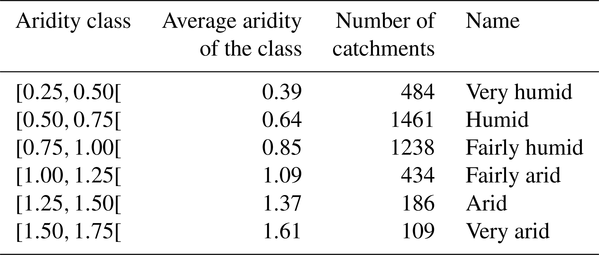
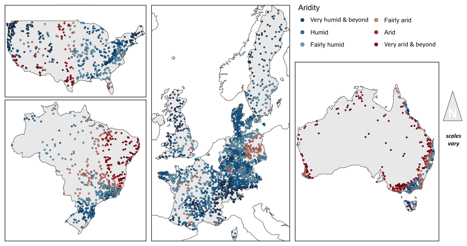
Figure 2 Location of the catchments studied and repartition by aridity classes.

2.2 Computation of local elasticities

Our reference method will consist in the local (i.e., catchment-specific) computation of streamflow elasticities using Eq. (16):

$$\begin{array}{}\text{(16)}& \mathrm{\Delta }{Q}_n=e_{Q/P}^{\text{loc}}\mathrm{\Delta }{P}_n+e_{Q/E_{\mathrm{0}}}^{\text{loc}}\mathrm{\Delta }{E}_{{\mathrm{0}}_n}+e_{Q/\mathrm{\Lambda }}^{\text{loc}}\mathrm{\Delta }{\mathrm{\Lambda }}_n\end{array}$$

Because the elasticity coefficients are obtained through linear regression, they are associated with statistical uncertainty, which we assess using the p-value. A significance threshold must be chosen, above which a coefficient is not considered statistically different from zero. For this paper, we use a conventional threshold of 0.05.

With this local approach, a unique triplet of elasticities is computed for each of the 4122 catchments, and the goodness of fit for each regression is, by definition, maximized (hence our choice of the local calibration as reference).

Note that the correlation between the independent variables of the regression presented in Eq. (16) is rather limited: the correlations computed at the catchment scale are comprised for 90 % of the cases in the range $[-\mathrm{0.6},\mathrm{0.2}]$ for $\left(\mathrm{\Delta }{P}_n\mathrm{\Delta }{E}_{{\mathrm{0}}_n}\right)$, in the range $[-\mathrm{0.7},\mathrm{0.5}]$ for (ΔP_nΔΛ_n), and in the range $[-\mathrm{0.5},\mathrm{0.4}]$ for $\mathrm{\Delta }{E}_{{\mathrm{0}}_n}\mathrm{\Delta }{\mathrm{\Lambda }}_n$),

2.3 Computation of unique elasticities by aridity class and for the entire dataset

We can also estimate a single triplet of elasticities for each different aridity class (as defined in Table 2) and we then use Eq. (17) for all the catchments of the given aridity class.

$$\begin{array}{}\text{(17)}& \mathrm{\Delta }{Q}_n=e_{Q/P}^{\text{cl}}\mathrm{\Delta }{P}_n+e_{Q/E_{\mathrm{0}}}^{\text{cl}}\mathrm{\Delta }{E}_{{\mathrm{0}}_n}+e_{Q/\mathrm{\Lambda }}^{\text{cl}}\mathrm{\Delta }{\mathrm{\Lambda }}_n\end{array}$$

Estimating a single triplet of elasticities for each class allows investigating the dependency of elasticity to aridity. To calibrate the three parameters, we use a simple grid search algorithm, exploring the following intervals: $[-\mathrm{0.1},\mathrm{1.1}]$ for $e_{Q/P}^{\text{cl}}$, and $[-\mathrm{1.1},\mathrm{0.1}]$ for $e_{Q/E_{\mathrm{0}}}^{\text{cl}}$ and $e_{Q/\mathrm{\Lambda }}^{\text{cl}}$, first with a coarse step of 0.1 and then a finer step of 0.01 around the optimum The objective function to be maximized is the bounded Nash–Sutcliffe Efficiency of Mathevet et al. (2006), which is first calculated for each catchment separately, and then averaged over the catchments belonging to the class and used as the objective to maximize (see Sect. 2.5).

For reference, we also compute a single triplet of elasticities at the global scale by pooling all 4122 catchments together. By construction, this world-wide triplet yields the lowest mean efficiency.

2.4 Computation of regionalized elasticities

In the regionalized approach, we use the entire dataset to calibrate a single underlying model, similarly to the calculation of elasticities at the global scale. However, this method ultimately produces catchment-specific results. Each catchment has a distinct triplet of elasticities because the elasticities for precipitation ($e_{Q/P}^{\text{reg}}$) and potential evaporation ($e_{Q/E_{\mathrm{0}}}^{\text{reg}}$) are modeled as functions of each catchment's aridity index (φ), given by Eq. (18). The regionalization formulas are adjusted by a shape parameter noted α:

$$\begin{array}{}\text{(18)}& \begin{array}{rl}{\displaystyle }\mathrm{\Delta }{Q}_n& {\displaystyle }=e_{Q/P}^{\text{reg}}\mathrm{\Delta }{P}_n+e_{Q/E_{\mathrm{0}}}^{\text{reg}}\mathrm{\Delta }{E}_{{\mathrm{0}}_n}+e_{Q/\mathrm{\Lambda }}^{\text{reg}}\mathrm{\Delta }{\mathrm{\Lambda }}_n\\ {\displaystyle }{e}_{Q/P}^{\text{reg}}& {\displaystyle }=f_P({\mathit{\alpha }}_P,\mathit{\phi })\\ {\displaystyle }{e}_{Q/E_{\mathrm{0}}}^{\text{reg}}& {\displaystyle }=f_{E_{\mathrm{0}}}({\mathit{\alpha }}_{E_{\mathrm{0}}},\mathit{\phi })\\ {\displaystyle }{e}_{Q/\mathrm{\Lambda }}^{\text{reg}}& {\displaystyle }=\text{constant}\left(\text{does not depend on }\mathit{\phi }\right)\end{array}\end{array}$$

There were several alternatives available for choosing the shape of functions f_P, and $f_{E_{\mathrm{0}}}$, as well as for adjusting the shape parameters. For f_P and $f_{E_{\mathrm{0}}}$ we used the derivatives of the Oldekop formula (see Eqs. 8 and 9). The variation range for these functions was constrained based on the results of the class calibration (Sect. 2.3). The synchronicity elasticity ($e_{Q/\mathrm{\Lambda }}^{\text{reg}}$) was kept constant because no clear empirical relationship was observed when examining either the local or the class-calibrated elasticities.

Figure 3 illustrate the dependency of streamflow elasticities to aridity, which is apparent both with the locally- and the class-estimated values. To keep the number of adjusted parameters low, we adjusted only three parameters (α_P, ${\mathit{\alpha }}_{E_{\mathrm{0}}}$ and $e_{Q/\mathrm{\Lambda }}^{\text{reg}}$) for Eq. (18), the variation bounds were set up empirically once for all based on the results of the class calibration.

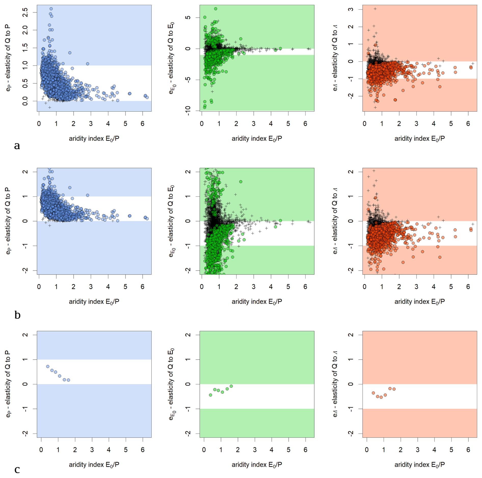
Figure 3 Relationship between the aridity index and locally-estimated climatic elasticities of streamflow, for precipitation elasticity (left), potential evaporation elasticity (middle), synchronicity elasticity (right). The white domain indicates the physically-plausible range (i.e. [0,1] for precipitation elasticity and $[-\mathrm{1},\mathrm{0}]$ for potential evaporation and synchronicity elasticities. (a) – (upper panel) Locally calibrated elasticity coefficients, showing all catchments (elasticities coefficients non-significant at the 0.05 level are figured as crosses), (b) – (middle panel) same as (a) with a zoom on the $[-\mathrm{2},\mathrm{2}]$ range; (c) – (lower panel) class calibrated elasticity coefficients (from Table 3).

2.5 Model evaluation criterion

To evaluate the performance of the different elasticity models in simulating streamflow anomalies, we use the classical Nash and Sutcliffe (1970) efficiency criterion (NSE). The NSE is usually computed for each of the 4122 catchments separately using Eq. (19):

$$\begin{array}{}\text{(19)}& \text{NSE}=\mathrm{1}-{\displaystyle \frac{{\sum }_n{\left(\mathrm{\Delta }{Q}_n^{\text{obs}}-\mathrm{\Delta }{Q}_n^{\text{cal}}\right)}^{\mathrm{2}}}{{\sum }_n{\left(\mathrm{\Delta }{Q}_n^{\text{obs}}-\stackrel{\mathrm{‾}}{\mathrm{\Delta }{Q}^{\text{obs}}}\right)}^{\mathrm{2}}}}\end{array}$$

Because the NSE varies in the interval $]-\mathrm{\infty },\mathrm{1}]$, it is not recommended to compute an average over large sets (indeed, a few very low criteria values will impact the average criterion value). For this reason, we follow Mathevet et al. (2006) and use the bounded form (called “C2M” in the original paper) as in Eq. (20):

$$\begin{array}{}\text{(20)}& \text{Bounded NSE (C2M)}={\displaystyle \frac{\text{NSE}}{\mathrm{2}-\text{NSE}}}\end{array}$$

3 Results

3.1 Empirical verification of the dependency between locally-estimated streamflow elasticities and aridity

We first computed the local streamflow elasticities for each catchment by linear regression (Eq. 16). Choosing an (arbitrary) significance level equal to 0.05, our dataset yielded 97 % of the catchments with a significant $e_{Q/P}$ parameter, but only 23 % of the catchments with a significant $e_{Q/E_{\mathrm{0}}}$ parameter, and 64 % of the catchments with a significant $e_{Q/\mathrm{\Lambda }}$ parameter.

Figure 3 presents the link between aridity and the locally-estimated elasticity coefficients. The results confirm the expected dependency between precipitation elasticity and aridity, which was previously shown for the theoretical formulas in Fig. 1. For the potential evaporation elasticity, a satisfying trend is visible but many physically unrealistic elasticities show that additional constraints are required for this term. Finally, the Λ-elasticity of streamflow (i.e. the streamflow elasticity towards the synchronous amounts of precipitation and streamflow), shows no clear dependency on the aridity index (but we did not expect any relationship).

3.2 Results by aridity class

We also calibrated the three elasticity coefficients to obtain a single triplet of values for each of the aridity classes as defined in Sects. 2.4 and 3.2. The resulting class-calibrated values are presented in Table 3. As reference, the performance of the local (catchment-specific) estimation is also provided (by construction, it represents the upper limit of performance).

Table 3 Class-calibrated elasticity values for catchments grouped by the aridity index φ.

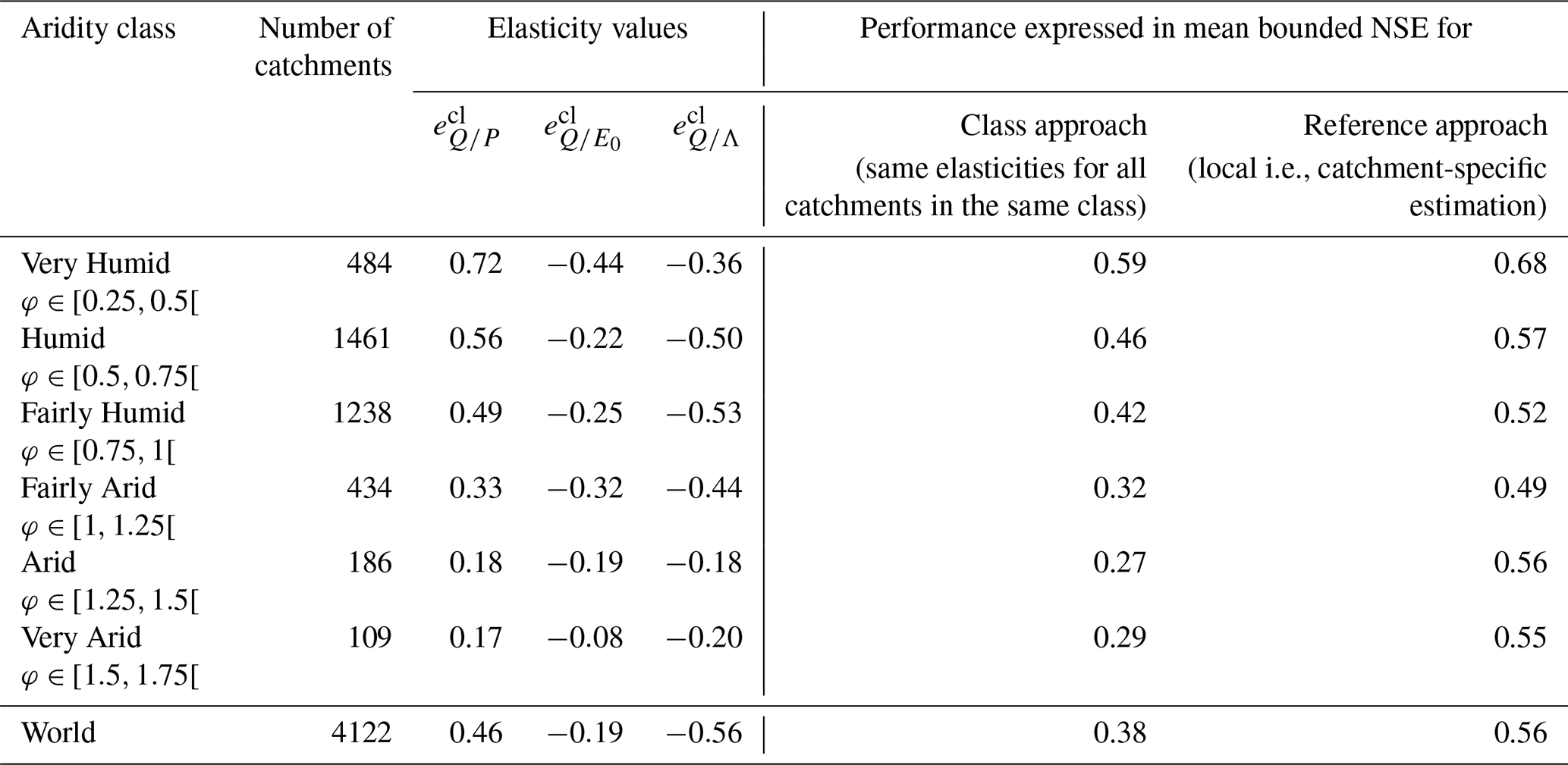
The numeric values in Table 3 confirm the tendency identified in Fig. 3: the precipitation elasticity of streamflow shows a clear decreasing trend with increasing aridity, while the potential evaporation elasticity shows a symmetric increasing trend. The empirical range of variation observed in the class-calibrated results is narrower than the theoretical range from the water balance formulas: for $e_{Q/P}$, the observed range is [0.17,0.72] compared to the theoretical [0,1], and for $e_{Q/E_{\mathrm{0}}}$, the range is $[-\mathrm{0.44},-\mathrm{0.08}]$ compared to the theoretical $[-\mathrm{1},\mathrm{0}]$. Finally, there is no clear trend identifiable for $e_{Q/\mathrm{\Lambda }}$. A clear advantage of the class-based calibration approach is that all resulting elasticities values fall, without exception, within the physically-realistic ranges.

3.3 Constraining the elasticity estimation with an aridity-dependent formulation: test for the entire dataset

The observed link between the aridity index and the local elasticity estimates suggested us to test the solution presented in Sect. 2.4, using a “regionalized” estimation of the elasticities of streamflow. This approach makes use of the identified pattern to enforce physical coherence across the entire dataset. To parameterize this relationship, we adapted the partial derivative of the parameter-free Oldekop formula (Table 1). We constrained the output of the Oldekop formulas to the empirical range observed in the class-based calibration (Table 3), offsetting the range for e_P to [0.15,0.75], and for $e_{E_{\mathrm{0}}}$ to $[-\mathrm{0.45},-\mathrm{0.10}]$. Thus, the regionalized elasticities are calculated as:

$$\begin{array}{}\text{(21)}& {\displaystyle }& {\displaystyle }\begin{array}{rl}{\displaystyle }& {\displaystyle }{e}_{Q/P}^{\text{reg}}=\mathrm{0.15}+|\mathrm{0.75}-\mathrm{0.15}|\cdot f_{P-\text{Oldekop}}({\mathit{\alpha }}_P,\mathit{\phi })\\ {\displaystyle }& {\displaystyle }\text{where}{f}_{P-\text{Oldekop}}\text{is given by Eq. (8)}\end{array}\text{(22)}& {\displaystyle }& {\displaystyle }\begin{array}{rl}{\displaystyle }& {\displaystyle }{e}_{Q/E_{\mathrm{0}}}^{\text{reg}}=-\mathrm{0.10}+|-\mathrm{0.45}+\mathrm{0.10}|\cdot f_{E_{\mathrm{0}}-\text{Oldekop}}({\mathit{\alpha }}_{E_{\mathrm{0}}},\mathit{\phi })\\ {\displaystyle }& {\displaystyle }\text{where}{f}_{E_{\mathrm{0}}-\text{Oldekop}}\text{is given by Eq. (9)}\end{array}\end{array}$$

Note that the restricted ranges remain within the physically-realistic limits.

We can now compare the performance of three modeling approaches: the “upper reference” where elasticities are calibrated locally at the catchment scale, the regionalized approach, and a “lower reference” with elasticities calibrated at global scale. While the upper reference requires the estimation of 12 366 parameters (3 elasticities for 4122 catchments), the latter two require only 3 parameters each. The corresponding results are presented below in Table 4 and Fig. 4.

Table 4 Results of the application of the regionalized approach to all the catchments of our dataset (4122): the performance is compared to a upper reference (with locally calibrated elasticity values) and a lower reference (with a unique value calibrated for all the catchments in the world).

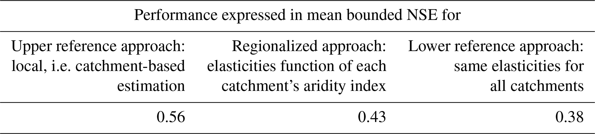
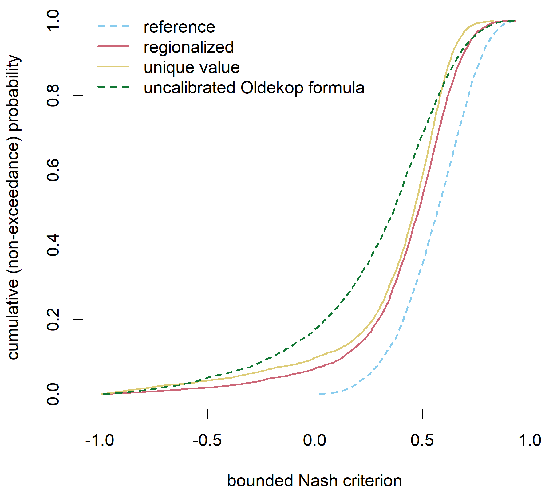
Figure 4 Distribution of the performances of the options compared in our paper, with the addition of the uncalibrated theoretical formulation derived from the Oldekop formula. The (unreachable) upper reference at the extreme right is followed by our regionalized solution, which has a better performance than an elasticity formula with a unique value (that would be independent from aridity) or than the elasticities derived from the (uncalibrated) Oldekop formula.

There is a clear advantage for taking into account the aridity in the regionalized formula. This approach covers 28 % of the performance gap between the lower and upper references, while using only three parameters. In addition, all elasticity parameters remain within the physically-realistic range. The proposed parametrization is therefore successful from both explanatory and predictive point of views, which is a clear advantage (Andréassian, 2023).

4 Discussion

In this paper, our aim was two-fold: (i) to empirically verify that at the catchment scale, streamflow elasticity and climate aridity are linked, and (ii) to propose an aridity-dependent parameterization allowing for the quantification of elasticity.

4.1 The need for an empirical verification

Because of the present popularity of Budyko's framework and its associated theoretical formulas (Table 1), an empirical verification of the elasticity-aridity link might appear superfluous. However, applying these theoretical formulas, such as the Oldekop derivative, relies on a “space-for-time-trade” assumption. This consideration assumes that a model validated across different spatial locations will also be valid for those locations for different time periods (see Peel and Blöschl, 2011, and Singh et al., 2011).

Berghuijs and Woods (2016) have warned that this trade requires validation, and Berghuijs et al. (2020) stress that although the Budyko-type curves have been used to predict the evolution of catchments in response to climatic changes, they originate from “observations of spatial differences in long-term water balances, and not from observations or theory of how individual catchments respond to aridity changes”. Thus, we argue that the elasticity-aridity link cannot be taken for granted and requires empirical verification, especially given the mixed results reported by Oudin and Lalonde (2023), who tested the classical space-time trading when parametrizing a land use dependent hydrological model, which failed to efficiently predict the direction and magnitude of hydrological changes after land use conversions.

4.2 An aridity-dependent parameterization that uses the shape of the Oldekop formula

Regarding our parameterization, our results confirm the general shape of the elasticity-aridity relationship given by the Oldekop formula, but they use a narrower range of variation than the theoretical one. Our work is therefore only partially coherent with the theoretical Budyko-type formulas, which appear to provide a wider range of elasticity values than our empirical data support. This should not be a surprise to hydrologists who know in particular how precipitation intensities impact the hydrological response of arid catchments. What is remarkable, however, is that the intuition of Schreiber (1904) and Oldekop (1911), embedded in formulas of elegant simplicity, remain so useful in the 21st century. We agree on this point with Zhang and Brutsaert (2021) who suggested that the “Budyko hypothesis” could justifiably have been named after Schreiber and Oldekop, who, with so little data and only slide rules, were able to imagine tools still in use today.

Concerning the difference between the elasticities derived from the theoretical Budyko-type formulas and the empirical class-calibrated values, we can suggest two explanations: first, a Budyko-type formula will always remain a conjecture (an elegant, mathematically relevant one but nevertheless, still a conjecture); second, Gnann et al. (2026) have shown that realistic observational noise will introduce systematic departures from the theoretical optimum.

5 Conclusion

5.1 Summary

In this paper, we investigated the dependency between streamflow elasticity and aridity using a large dataset of 4122 catchments across Europe, Australia, North America and South America. Our analysis confirmed the well-established dependency between elasticity and aridity and showed that the shape of this dependency can be effectively reproduced by existing theoretical formulas. We further demonstrated that these theoretical formulas can be used to guide the regionalization process, producing a regionalized aridity-dependent estimate of streamflow elasticity for each catchment, based on a parsimonious parameterization. The proposed solution, based on the Oldekop formula, is summarized in Table 5 below and illustrated in Fig. 5.

Table 5 Summary of the proposed aridity-accounting regionalized formulas for computing the precipitation and potential evaporation elasticities of streamflow. ΔQ, ΔP, ΔE₀ and ΔΛ are the annual streamflow, precipitation, potential evaporation and synchronicity anomalies, respectively [mm yr⁻¹]. The nondimensional aridity index ($\mathit{\phi }=\stackrel{\mathrm{‾}}{E_{\mathrm{0}}}/\stackrel{\mathrm{‾}}{P}$) is computed as a long-term average. f_P(φ) and $f_{E_{\mathrm{0}}}\left(\mathit{\phi }\right)$ are borrowed from the Oldekop formula (see Table 1).

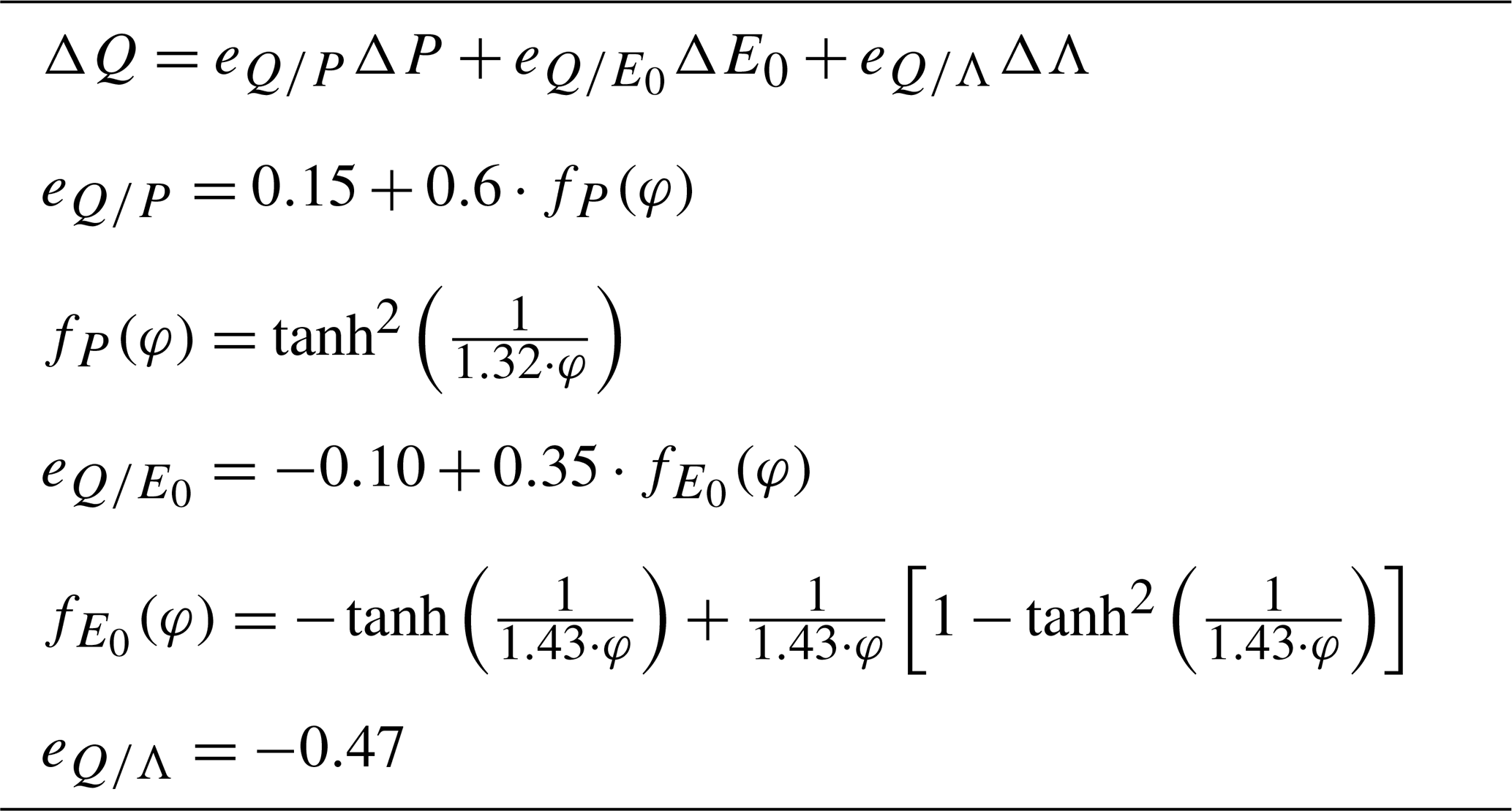
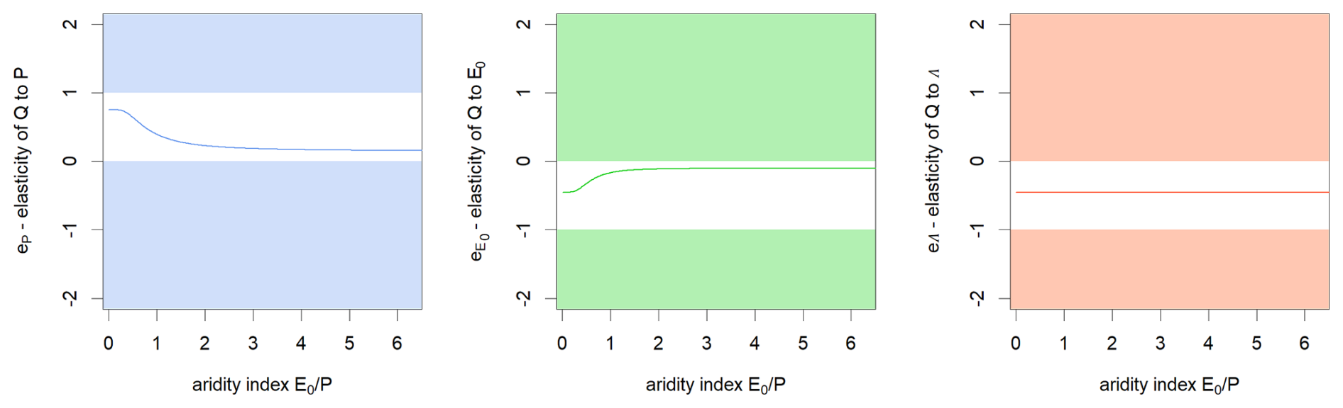
Figure 5 Regionalized relationships (from the equations in Table 5) for the climatic elasticities of streamflow as a function of the aridity index: precipitation elasticity (left), potential evaporation elasticity (middle), synchronicity elasticity (right). The white domain indicates the physically-plausible range, i.e. [0,1] for precipitation elasticity and $[-\mathrm{1},\mathrm{0}]$ for potential evaporation and synchronicity elasticities.

5.2 Limitations and perspectives

Because our work was empirical, and even if it is based on a very large set of real-world data, it will remain provisory, until improved by others. It is important to note three limitations in our study. First, the relationships in Table 5 were developed on catchments with limited interannual memory (in the sense of de Lavenne et al., 2022): this excludes those catchments for which Eq. (3) would not be warranted to estimate streamflow elasticity, since additional independent variables expressing the climatic anomalies of the previous years would have been required. This could have been done following the work of de Lavenne et al. (2022), or of Pelletier and Andréassian (2020), but we preferred to keep the elasticities' estimation as simple as possible. Second, aridity was computed using the Oudin et al. (2005) formula for potential evaporation, and the use of other formulas might require a recalibration of the model parameters. Third, although we do believe that aridity is the first-order driver of elasticity at the global scale, it is not the only one, and our regional model is clearly only a first step in the search for physical explanations.