Exploring groundwater-surface water interactions and recharge in fractured mountain systems: an integrated approach

This study presents an integrated approach to map groundwater-surface water (GW-SW) interactions in a scarcely anthropized Mediterranean mountain catchment (Ussita) characterized by fractured limestone rocks with complex spatial-temporal patterns of hydrological processes. Understanding GW contributions to streams like the Ussita is crucial for addressing environmental challenges, including water resources management and evaluating ecological flows to protect aquatic ecosystems. The use of traditional hydrological techniques, such as discharge measurements along various stream reaches, combined with hydrochemical-isotopic analyses and innovative thermal drone surveys, enabled us to quantify the specific contributions of different limestone aquifers to sustaining streamflow. Integrating satellite-based meteorological datasets with in-situ observations further helped to constrain the water budget and assess the extent of the recharge area. Hydrogeological analyses also revealed that snowmelt contributes about 18 % to aquifer recharge, an important consideration for GW availability in the face of future spatial-temporal changes in snow patterns. These findings can support further studies in other catchments by guiding and optimizing field campaigns to identify site-specific conditions responsible for GW inflow, from point sources to stream reaches. Moreover, the results can help optimize resource management, mitigate climate-related risks, and support the long-term sustainability of both upstream and downstream socio-ecological systems.

1 Introduction

Carbonate aquifers in mountainous regions host strategic groundwater (GW) resources that interact dynamically with surface water (SW), influencing the quantity and quality of downstream water bodies. In such systems, baseflow (BF), the portion of streamflow derived from GW seeping into streambeds, is a key component of discharge, especially during no-recharge periods, such as prolonged droughts or seasonal dry spells typical of the Mediterranean Region (Winter, 2007; Duncan, 2019). According to a recent report by the Italian Institute of Statistics (https://esploradati.istat.it/databrowser/#/en/dw/categories/IT1,Z0920ENV,1.0/ENV_WATER, last access: 30 July 2025.), drinking water for about 12 million people is supplied by groundwater resources (92 %), the main source of which is springs fed by fractured-karst limestone aquifers located at medium-to-high altitudes along the Apennine ridge. Despite their importance, many mountainous hydrogeological systems are increasingly stressed by overexploitation and climate change (Rateb et al., 2020).

In mountainous hydrogeological systems, GW-SW interactions can be very complex with variations in GW storage strongly influencing stream discharge (Scanlon et al., 2023), water temperature (White et al., 2023), and water quality (Conant Jr. et al., 2019). The characterisation of GW and SW interactions is therefore paramount for water resource management and for managing environmental water resource challenges, such as specifying ecological flows to preserve aquatic ecosystems (Acreman and Dunbar, 2004; Lorenzoni et al., 2019; Fernández-Martínez et al., 2023). Furthermore, characterizing GW contributions supports the comprehension of processes regulating rocks' physical and chemical weathering, a key process of the global carbon cycle, both in the long- and the short-term (see e.g. Kump et al., 2000; Tipper et al., 2006; Hartmann et al., 2009; Hilton and West, 2020).

Understanding GW–SW exchange in streams is not straightforward and often requires treating them as a single, integrated resource rather than separate components. As reported by Muñoz et al. (2024), understanding GW contributions from mountain aquifers that ultimately sustain streamflow remains limited (Somers and McKenzie, 2020) and understudied due to many uncertainties related to scarce information and the high cost of obtaining reliable data (Somers and McKenzie, 2020; Adler et al., 2023). Regional variations in climate, snowpack, and catchment characteristics further complicate generalizations of GW-SW interactions in mountain regions of the Mediterranean, where several geological interplaying factors, including fracturing and karst features, increase the complexity of GW systems and thus their management (e.g., Preziosi, 2007; Cambi et al., 2010; Boni et al., 2010; Di Matteo et al., 2020; Lancia et al., 2020; Preziosi et al., 2022; Azimi et al., 2023; Xanke et al., 2024). These features also render quantitative studies through groundwater modeling intricate, as the boundary conditions are difficult to constrain, inter-aquifer exchanges may be significant, and hydrogeological parameters are hard to estimate in heterogeneous carbonate massifs (e.g., Silberstein, 2006; Beven, 2007; Clark et al., 2017; Azimi et al., 2023). As a result, physically based models may remain poorly constrained, or even unfeasible, without a minimum level of monitoring data beyond plot and hillslope scales. Currently, several opportunities are offered by new Earth Observation (EO) data, such as GRACE (see Rodell and Famiglietti, 2002, and the literature therein); however, according to Yin et al. (2022), the use of EO data like GRACE, even integrated with models via data assimilation, typically yields underestimated depletion signals in mountain areas at very local scales. Therefore, expanding mountain-based networks of meteorological and streamflow observations remains essential (Dettinger, 2014). Collecting accurate streamflow and hydrometeorological data in mountainous terrain is logistically difficult and costly (Shakti and Sawazaki, 2021), making it challenging to understand where aquifer-stream interactions or GW outflows towards neighbouring systems occur, the latter complicated by fault zones and karst features, which strongly govern GW circulation in mountain aquifer systems (e.g., Ofterdinger et al., 2019). This is especially true for the European Mediterranean region (Polo et al., 2020), which is considered a major global “hotspot” for climate change, with projections showing it will face more severe, frequent, and long-lasting droughts in the coming decades (Tramblay et al., 2020). This is a key point that requires collecting data to develop reliable water budgets and to acquire hydrogeological properties of aquifers (Bonacci, 1993; Dragoni et al., 2013; Di Matteo et al., 2017, 2020; Valigi et al., 2021). Closing the water budget in mountainous catchments remains a persistent challenge due to data requirements and scale-dependent uncertainties (Levin et al., 2023; Marti et al., 2023). Therefore, it is important to characterize the exchanges between GW and SW. Recently, Zheng et al. (2025) highlighted that the non-closure of the water budget exhibits clear scale-dependent behavior and is strongly influenced by hydro-meteorological conditions. For instance, underestimating cold-season precipitation (including snowfall and subsequent snowmelt) or warm-season evapotranspiration can cause under- or overestimation of groundwater recharge, a problem particularly relevant in Mediterranean mountainous catchments. However, only a few studies have investigated and quantified the role of snowmelt in aquifer recharge in Mediterranean environments (Fayad et al., 2017) and, specifically, in the Apennine region (Lorenzi et al., 2023; Rusi and Di Giovanni, 2024). To date, most studies investigating GW–SW interactions in Mediterranean mountain carbonate catchments rely on single data streams (e.g., discharge records, local hydrochemical data, or model-based reconstructions). This limits the ability to understand the water budget and to accurately determine recharge areas and groundwater contributions to streamflow. Here, we address this challenge by proposing an integrated methodological framework that combines remote sensing, in situ hydrometeorological monitoring, streamflow observations, and environmental tracers to jointly estimate recharge and groundwater inflows to streams. The novelty of this work lies in the integration strategy and workflow, designed to be applicable to other data-scarce mountainous carbonate regions facing increasing drought stress. Specifically, we address the following research questions:

• a.

  How can the integration of EO data, in situ observations, and tracers improve the quantification of groundwater inflow to streams and the delineation of recharge areas compared with streamflow data alone?

• b.

  What is the role of snow accumulation and melt in controlling aquifer recharge and sustaining dry-season baseflow in Central Apennine carbonate catchments?

We demonstrate this approach in the Ussita stream catchment (44 km²), a mountain catchment located along the Central Apennine Ridge (Italy). The catchment is minimally affected by human activities (e.g., groundwater withdrawals or stream diversions). A small hydropower station in the mid–upper catchment operates intermittently (a few hours per week) and produces negligible effects on stream discharge. Continuous discharge monitoring is complemented by spot discharge measurements, thermal-drone surveys, GW and SW tracer tests, and geochemical and isotopic sampling. Together, these observations make Ussita an experimental catchment for investigating natural GW–SW exchange processes and quantifying the spatial variability of baseflow contributions along the stream reach.

Although developed for the Ussita catchment, the methodology is designed to be adaptable to other Mediterranean mountain catchments and to fractured systems worldwide with limited high-elevation monitoring. This aids in achieving a comprehensive understanding of mountain hydrological systems, optimizing resource management, mitigating climate-related risks, and supporting the long-term sustainability of both upstream and downstream socio-ecological systems.

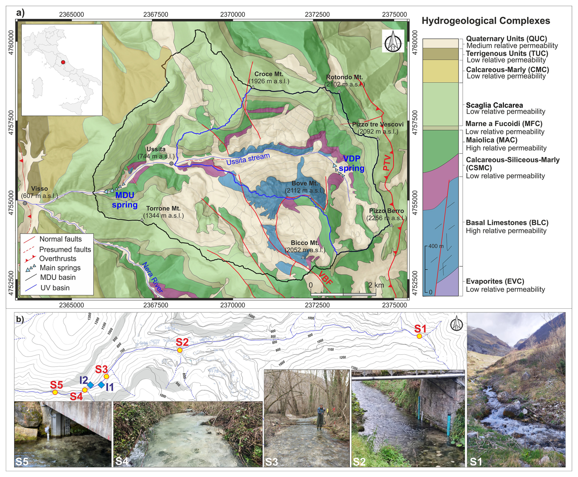
Figure 1 (a) Map of the hydrogeological complexes of the Ussita stream catchment area as derived by new hydrogeological surveys that have supplemented the geological study by Pierantoni et al. (2013). MDU = Ussita catchment at Madonna Dell'Uccelletto (MDU); UV = Ussita catchment at Ussita Village (UV); VDP = Val Di Panico spring; VBF = Mt. Vettore-Mt. Bove Fault system; PTV = Pizzo Tre Vescovi thrust. (b) The location of stream gauges with reliable rating curves (S2 and S5), stream sections monitored by spot measurements with the OTT MF Pro flow meter (S1, S3, and S4), and GW inflow (I1 and I2). The grey shadow zone represents the outcropping of the low-permeability Marne a Fucoidi Complex (MFC).

2 Materials and methods

2.1 The Ussita experimental catchment

The Ussita catchment is situated along the Apennine ridge of Central Italy and is characterized by carbonate multilayer formations belonging to the Umbria-Marche stratigraphic sequence. Figure 1a shows the geological map of the study area with the location of two nested study catchments. The catchment outlet at Madonna dell'Uccelletto (MDU) drains an area of 44 km² (S5 in Fig. 1b), whereas the stream in the upper part at Ussita Village (UV) drains 18 km² (S2 in Fig. 1b). The mean altitude of MDU is about 1315 m a.s.l., while the maximum and minimum altitudes are about 2256 m and 645 m a.s.l., respectively. The carbonate sequence lies on Upper Triassic evaporitic rocks, primarily composed of low-permeability anhydrites and dolomites (Evaporites Complex, EC). However, these units are not exposed in the area under investigation. Owing to the presence of shallow-water carbonate deposits and pelagic formations, the Ussita catchment is characterized by hydrogeological complexes with a range of different relative permeabilities (right-hand column in Fig. 1a). More specifically, there are two high-permeability complexes: the Basal Limestones Complex (BLC, composed of the Calcare Massiccio and Corniola formations) and the Maiolica Complex (MAC). They host important aquifers due to strong fracturing and karstification (for BLC). BLC and MAC are separated by the Calcareous Siliceous Marly Complex (CSMC), which has relatively low permeability and is composed of formations deposited in a structural low (Rosso Ammonitico, Marne del Serrone, Calcari a Posidonia, and Calcari Diasprigni formations) and in a structural high (Bugarone). The latter outcrops in a small tectonic window in the lowest part of the MDU catchment, close to the Madonna dell'Uccelletto spring (I2 in Fig. 1b). Above the MAC lies the Marne a Fucoidi Complex (MFC), a marly deposit of low-permeability rocks. Subsequently, marly limestone units exhibit moderate permeability and include the Scaglia Rossa and Scaglia Bianca formations (Scaglia Calcarea Complex, SCC). These are overlain by the Scaglia Variegata and Scaglia Cinerea formations, composed of marls and marly limestones, which also have low permeability and are grouped as the Calcareous Marly Complex (CMC), outcropping outside the MDU catchment. In the eastern part of the study area, Miocene-aged marly units (Schlier and Bisciaro) and the siliciclastic Laga Formation are predominant. These formations are part of the Terrigenous Units Complex (TUC) and typically exhibit moderate to low permeability.

Multiple tectonic events beginning in the Jurassic influenced all the formations described above, involving both extensional and compressive phases. Concerning the compression structures (Miocene-Pliocene), a key feature is the Pizzo Tre Vescovi Thrust (PTV), located in the eastern part of the study area (Fig. 1a). A system of NNW–SSE trending normal faults that developed from the Late Pliocene Quaternary extensional tectonic phase intersected later compressive structures. These faults are still active, contributing to the seismicity of the area, the latter of which occurred on 30 October 2016 (M_w 6.5), about 15 km south of Ussita Village, triggered by the rupture of different segments of the Vettore Mt.–Bove Mt. Fault system, VBF (e.g., Brozzetti et al., 20199). This seismic sequence deeply affected the hydrogeological properties of aquifers in the headwaters of the Nera River, into which the Ussita stream flows (Fig. 1), by different transient co-seismic effects such as the release of crustal fluids following elastic co-seismic deformations, the increase in water pressure following the rise in the hydraulic gradient in the aquifer, and the changes in rock permeability due to microcracks, unblocking of pre-existing fractures, and fracture cleaning (Petitta et al., 2018; Di Matteo et al., 2020, 2021; Mastrorillo et al., 2020, 2023; Cambi et al., 2022). However, according to Di Matteo et al. (2021), starting in 2019, pre-seismic conditions have recovered, and total river flow can be analyzed in the context of the meteo-climatic processes that regulate GW-SW interactions.

2.2 Datasets and monitoring network

2.2.1 Ground-based hydrometeorological monitoring network

Daily stream levels of the Ussita stream were collected at the outlet of the two sub catchments investigated, S2 and S5, placed at the closure of the UV and MDU catchments, respectively (Fig. 1b). In detail, stream level data of the S5 section were collected from the SIRMIP online monitoring network (Civil Protection Agency of Marche Region, Central Italy). At the same time, those of S2 were made available thanks to the hydrological monitoring infrastructure available at the Sibillini National Park Critical Zone observatory (SINCZONE, https://cnr-eco-hydrology-lab.org/sinczone-observatory, last access: 29 July 2025), developed and managed by CNR-IRPI (Istituto di Ricerca per la Protezione Idrogeologica of CNR). Overall, the observation period for S5 was from 2019 to 2024, and for S2, this was from 2022 to 2024. For both stream gauges, the stream level data (H) were plotted against stream discharge data (Q) taken by the OTT MF Pro flow collected during the 2022–2025 period, yielding curves with the following metrics: S2 section (R²=0.957, RMSE =0.032 m³ s⁻¹); S5 section (R²=0.842, RMSE =0.054 m³ s⁻¹). Overall, the gauging sections exhibit stable channel geometry; thus, the reliability of the rating curves is rated as good (e.g., Tomkins, 2014). Moreover, during the 2022–2025 period, the spot discharge measurements by the OTT MF Pro flow were extended to stream sections S1, S3, and S4 (10 discharge measures in the range 0.70–1.18 m³ s⁻¹, Fig. 1b) to investigate GW inflow from limestone aquifers across the larger stream stretch. The spot stream discharge measurements were carried out in periods mostly falling within the recession curve, where baseflow contribution to the stream is dominant: it was possible by checking remotely the stream-level dataloggers (placed in stream sections S2 and S5 in Fig. 1). Combining continuous and discrete monitoring enabled us to develop robust analyses, which help us understand stream segments primarily fed by groundwater moving from the stream headwaters toward section S5.

The experimental setup included six ground-based weather stations (Table S1 and Fig. S1 in the Supplement). The Ussita and Casali stations measured temperature and rainfall data at hourly intervals inside the catchment, which were also aggregated to different timescales (hourly, daily, monthly, and yearly). As reported in Table S1, the Ussita station has the longest dataset and serves as a reference for characterizing mean precipitation over the Ussita catchment. As reported by Di Matteo et al. (2021) and Gentilucci et al. (2021), a substantial underestimation of precipitation at the Monte Bove Sud rain gauge relative to lower-elevation sites has been observed. Ussita, ENDESA, and Ponte Tavola rain gauges are used in this analysis, allowing us to demonstrate the unreliability of stations at high altitudes and to exclude them from the computation of precipitation over the catchment.

Snow depth was measured at two stations (Monte Bove Sud and Pizzo Tre Vescovi; see Fig. S1). However, during the investigation period, they exhibited substantial data gaps, rendering them unsuitable for analysis. It is a common issue in the mountain regions of the Italian Apennines and Alps, where the presence of precipitation and snow depth monitoring stations at higher elevations is scarce or not representative of the mean altitude of mountain catchments (Cambi et al., 2010; Daly et al., 2017; Ly et al., 2013; Di Matteo et al., 2017; Avanzi et al., 2024b; Girotto et al., 2024). Whereas the role of snowmelt cannot be neglected in the highest-elevation areas of Mediterranean catchments, which receive most of their winter/spring precipitation as snow, this is less of a concern in mid-elevation areas, which have a mixed precipitation regime (e.g., Fayad et al., 2017).

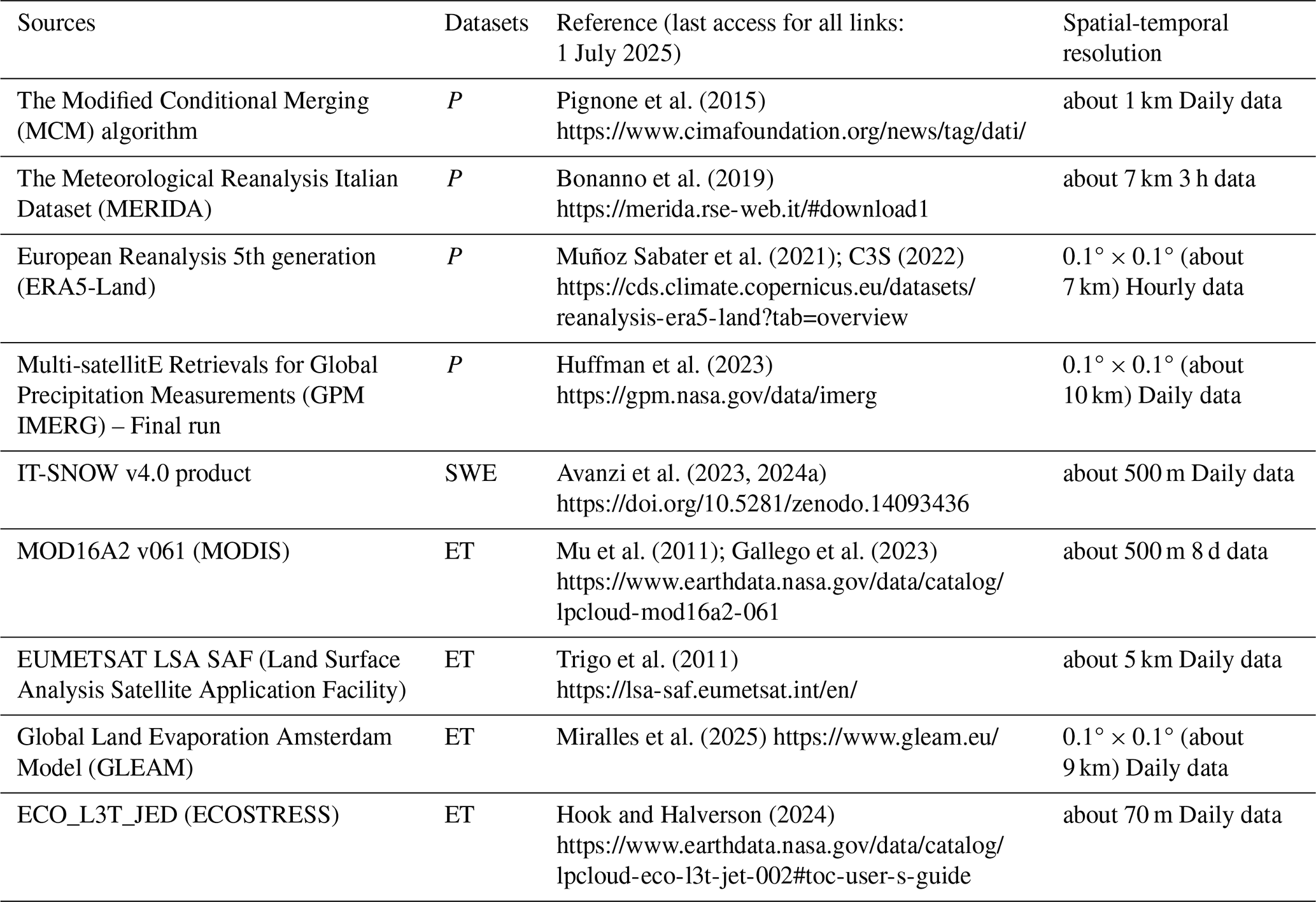
2.2.2 Hydro-meteorological regional and global datasets

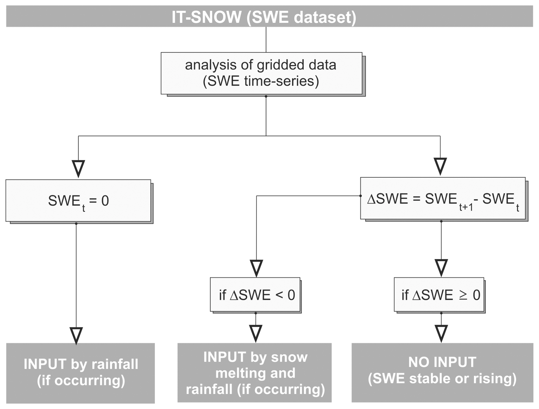
To address data scarcity, complementary precipitation (P) products were used to estimate rainfall (P_rain) and snowmelt (P_snow) at different spatial and temporal resolutions over the MDU catchment. Table 1 summarizes the basic characteristics of datasets at the regional and global scales. Snow Water Equivalent (SWE) data from the IT-SNOW dataset were used to extract and analyze monthly snowmelt contributions (P_snow) over the MDU catchment. The analysis was carried out following the workflow in Fig. 2. In detail, when SWE was zero (no snow), the precipitation (if present) was the only input to the system (P_rain). When snow cover was present, a day-by-day and cell-by-cell evaluation was conducted to assess changes in SWE relative to the previous day (ΔSWE). For ΔSWE <0, it was assumed that snowmelt occurred, contributing to P_snow.

Monthly Evapotranspiration (ET) was estimated and then aggregated at the hydrological-year scale using remote-sensing estimates (Table 1). Moreover, the Thornthwaite-Mather (T-M) method (Thornthwaite and Mather, 1955, 1957) was used to estimate ET from ground-based meteorological data (see Supplement Sect. S2). More detailed descriptions of the P, SWE, and ET products, along with uncertainty taken from the literature (when available), are provided in the Sect. S1.

Table 1 Basic characteristics of the datasets.

Figure 2 Workflow for analyzing water availability contribution from IT-SNOW's SWE data.

2.3 Baseflow separation

Among available indices, the Base Flow Index (BFI) is one of the most widely used metrics for assessing the contribution of baseflow to total streamflow (Nathan and McMahon, 1990; Smakhtin, 2001; Longobardi and Villani, 2023). BFI is defined as the ratio between mean annual baseflow (BF) and mean annual streamflow (Q). To compute BFI at sections S2 and S5, the BF component was separated from the observed streamflow hydrograph.

As recently discussed by Nagy et al. (2024), separating the hydrograph into baseflow and direct runoff is non-trivial because baseflow is rarely observed directly. Among the available techniques, digital filters (e.g., Furey and Gupta, 2001) provide an objective and reproducible approach that allows BF estimates to serve as diagnostic indicators of groundwater contribution to streamflow, rather than exact fluxes. Although the evaluation of BF separation methods remains an open question in the literature, Xie et al. (2020) showed that digital-filter methods perform well across 1145 catchments in the USA, including systems characterized by high infiltration rates, such as the Ussita catchment. Therefore, we adopted the one-parameter recursive digital filter proposed by Lyne and Hollick (1979) (Eq. 1), which provides an intuitively satisfactory representation of baseflow (e.g., Duncan, 2019) and has also been successfully applied in karst catchments (Mo et al., 2025). In this method, the baseflow at time t (B_t) is separated from the total stream discharge at time t (Q_t) using a filter parameter k that effectively separates low-frequency signals (associated with baseflow). Selecting an appropriate k-parameter value remains an open question, even though the Lyne and Hollick (1979) method is considered helpful for comparative hydrology and regionalization, as it can be used to consistently characterize differences between catchments (Ladson et al., 2013). According to Nathan and McMahon (1990), applying the Lyne and Hollick filter requires selecting several passes and a single k-parameter value. More specifically, the k-parameter affects the degree of baseflow attenuation, and the number of passes determines the degree of smoothing (Nagy et al., 2024). The k-parameter typically ranges from 0.90 to 0.99 (e.g., Kang et al., 2022). One of the main sources of uncertainty in digital filter methods is the linear reservoir assumption (Xie et al., 2020), which holds for the Ussita catchment because discharge during the recession period is described by the Maillet equation (e.g., Di Matteo et al., 2020; Mastrorillo et al., 2020). In this way, Chapman (1991) and Tan et al. (2009) linked the k value to the recession coefficient α ($k=e^{-\mathit{\alpha }t}$) estimated by the Master Recession Curve (MRC), considering daily or hourly discharge time steps (e.g., Tallaksen, 1995; Posavec et al., 2006; Gregor and Malik, 2012; Di Matteo et al., 2017, 2020; Carlotto and Chaffe, 2019). Following this approach, the k-parameter value for each catchment was estimated, and the recursive filter was applied by setting the number of passes to three (forward–backward-forward) to minimize phase distortion effects on the peak values (Nathan and McMahon, 1990). As reported by Kang et al. (2022), it is necessary to verify that the selected digital filter is appropriate for separating baseflow during the dry season (when baseflow represents stream discharge). In other words, to constrain baseflow estimates as effectively as possible, the BF data computed by the LH method must be validated against continuous streamflow data during no-recharge periods (S2 and S5 sections for the Ussita catchment).

$$\begin{array}{}\text{(1)}& B_t=k\cdot B_{(t-\mathrm{1})}+{\displaystyle \frac{\left(\mathrm{1}+k\right)}{\mathrm{2}}}(Q_t-Q_{t-\mathrm{1}})\end{array}$$

2.4 Water budget components and computation

The water budget is a key management tool that accounts for inflows, outflows, and changes in storage (ΔS) within a specific system over a given period. The following subsections (Sect. 2.4.1 and 2.4.2) detail a method for estimating the change in storage (ΔS) and the approach used to compute the water budget.

2.4.1 Estimation of the water storage changes (ΔS)

Water storage changes (ΔS) must be considered in hydrogeological analysis because the water budget spans four years (2019–2023), making it essential not to overlook this component. As is often the case in mountain systems, piezometric observations were unavailable for calculating ΔS in the Ussita catchment because the groundwater table is deep, and drilling costs and environmental constraints (i.e., the Ussita catchment is entirely within a National Park) limit the feasibility of such measurements. Under these conditions, stream recession analysis can help determine ΔS (e.g., Korkmaz, 1990; Dewandel et al., 2003; Malik and Vojtková, 2012; Płaczkowska et al., 2018). Since the Maillet equation accurately describes stream discharge data of the Ussita stream during no-recharge periods (Di Matteo et al., 2020; Mastrorillo et al., 2020), estimating water storage changes through recession analysis – despite its oversimplification – can still provide valuable insights, especially when included in the mean annual water budget (e.g., Tallaksen, 1995; Raeisi, 2008; Krakauer and Temimi, 2011). As noted by Hameed et al. (2025), baseflow recession analysis serves as a reliable, high-resolution proxy for monitoring groundwater storage. It is particularly useful in regions with limited well-level observation networks or where satellite data are too coarse for small watersheds, such as Ussita. Although the Korkmaz method has been in use for several decades, it remains relevant (e.g., Abirifard et al., 2022). In detail, for stream discharge described by the Maillet exponential relationship, it is possible to calculate the recession coefficient values (α) for each year (i). For example, considering the period from October to the following September, which includes two consecutive years (i and i+1), it is possible to compute the storage variation (ΔS) for each hydrological year using Eq. (2).

$$\begin{array}{}\text{(2)}& \mathrm{\Delta }S=V_m-V_{\mathrm{0}}=\mathrm{86}\mathrm{400}\cdot \left({\displaystyle \frac{Q_m}{{\mathit{\alpha }}_{i+\mathrm{1}}}}-{\displaystyle \frac{Q_{\mathrm{0}}}{{\mathit{\alpha }}_i}}\right)\end{array}$$

where ΔS= dynamic reserve change during the hydrological year. Q_m and V_m= streamflow and dynamic reserve at the end of the period. Q₀ and V₀= streamflow and dynamic reserve at the beginning of the period. α_i and $\mathit{\alpha }i+\mathrm{1}=$ recession coefficient for years i and i+1.

2.4.2 Water budget computation

Equations (3) and (4) mathematically express the water budget for a small catchment not affected by withdrawals or stream diversions towards other systems (Healy et al., 2007), as occurs for the MDU catchment. Each water budget term can be expressed as depth per unit time or volume per unit time (Mitsch and Gosselink, 2000).

$$\begin{array}{}\text{(3)}& {\displaystyle }P+Q_{\mathrm{in}}^{\mathrm{gw}}=\mathrm{ET}+\left(Q+Q_{\mathrm{out}}^{\mathrm{gw}}\right)+\mathrm{\Delta }S\text{(4)}& {\displaystyle }P-\mathrm{ET}=\mathrm{WS}=Q+\left(Q_{\mathrm{out}}^{\mathrm{gw}}-Q_{\mathrm{in}}^{\mathrm{gw}}\right)+\mathrm{\Delta }S\end{array}$$

where P= total precipitation. $Q_{\mathrm{in}}^{\mathrm{gw}}=$ groundwater inflow into the catchment. ET = actual evapotranspiration. Q= total streamflow at the closure of the catchment (surface runoff plus base flow). WS = water surplus. $Q_{\mathrm{out}}^{\mathrm{gw}}=$ groundwater outflow towards neighboring hydrogeological systems. ΔS= change in water storage.

The WS values in Eq. (4) have been computed for the 2019–2023 period by subtracting the mean precipitation (P) from the mean ET, using the various independent sources in Table 1. Moreover, the WS was computed using precipitation from the Ussita gauge and ET from the Thornthwaite-Mather method. WS estimates also included the BIGBANG 8.0 dataset “Nationwide GIS-Based hydrological budget on a regular grid” (Braca et al., 2024). Details about the BIGBANG product are in the Sect. S3.

The water outflow from the catchment ($Q+Q_{\mathrm{out}}^{\mathrm{gw}}$, in Eq. 5) represents the integrated response to all hydrogeological processes within the catchment (e.g., Singh and Woolhiser, 2002; Kirchner, 2009). According to Schaller and Fan (2009), under the assumption of no ΔS changes, a simple indicator of the partition of the water surplus (WS) is the $Q/\mathrm{WS}$ ratio. A $Q/\mathrm{WS}<$1 indicates that a portion of WS failed to emerge as stream outflow (i.e., the catchment drains water towards other systems, acting as a “groundwater exporter”). On the contrary, if $Q/\mathrm{WS}>\mathrm{1}$, the observed stream discharge must include groundwater inflow from the neighboring systems (i.e., the catchment must be a “groundwater importer”). Scanlon et al. (2002) proposed an expanded form of the water budget (Eq. 5) that accounts for two precipitation components: P_rain (liquid precipitation) and P_snow (snowmelt).

$$\begin{array}{}\text{(5)}& P_{\mathrm{rain}}+P_{\mathrm{snow}}+Q_{\mathrm{in}}^{\mathrm{gw}}=\mathrm{ET}+(Q+Q_{\mathrm{out}}^{\mathrm{gw}})+\mathrm{\Delta }S\end{array}$$

Equation (5) can be rewritten as follows (Eq. 6).

$$\begin{array}{}\text{(6)}& \begin{array}{rl}(Q_{\mathrm{in}}^{\mathrm{gw}}& -Q_{\mathrm{out}}^{\mathrm{gw}})=-(P_{\mathrm{rain}}-\mathrm{ET})-P_{\mathrm{snow}}+Q+\mathrm{\Delta }S=\\ & -(\mathrm{WS}+P_{\mathrm{snow}})+Q+\mathrm{\Delta }S\end{array}\end{array}$$

In Eq. (6), the water budget's only unknown component is ($Q_{\mathrm{in}}^{\mathrm{gw}}-Q_{\mathrm{out}}^{\mathrm{gw}}$), which is the residual, while the others can be measured (e.g., Q) or estimated (P_rain, P_snow, ET, and ΔS). According to Viaroli et al. (2018), quantifying groundwater exchanges in mountain regions is challenging since the system's boundary conditions are not defined. The geological-structural complexity of the Apennine chain (which includes the study area of this work) complicates the accurate assessment of groundwater inflows and outflows (Filippini et al., 2015). These hidden water budget components may constitute a considerable portion of groundwater availability (Carrillo-Rivera, 2000). Regardless, the unknown component of Eq. (6) ($Q_{\mathrm{in}}^{\mathrm{gw}}-Q_{\mathrm{out}}^{\mathrm{gw}}$) can be computed by introducing the measured and/or estimated components of the right side of Eq. (6). Considering the catchment area A as system, a value of $Q_{\mathrm{in}}^{\mathrm{gw}}-Q_{\mathrm{out}}^{\mathrm{gw}}\gg \mathrm{0}$ means that, net of uncertainties in the estimation of the water budget components, there is a groundwater inflow (i.e., the hydrogeological basin A^* is much larger than the catchment area A). Figure 3 shows a schematic hydrogeological system with groundwater inflow into the catchment ($A^{*}\gg A$).

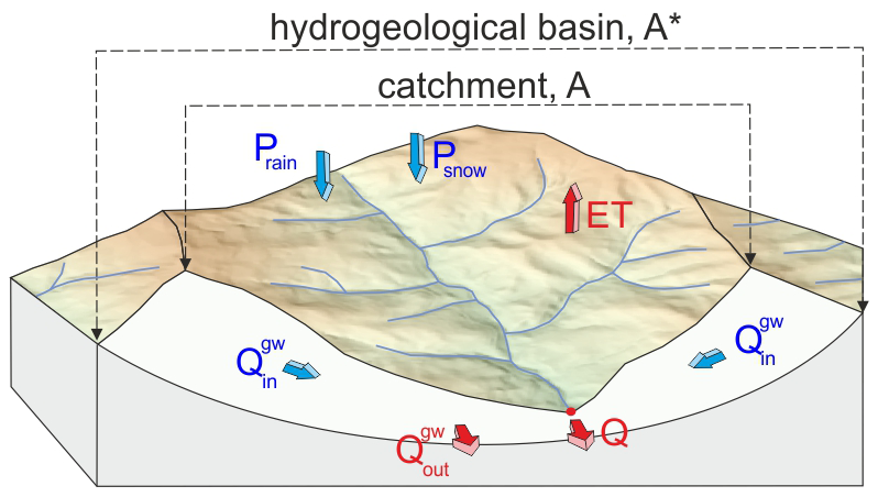
Figure 3 Schematic representation of a hydrogeological system with groundwater inflow coming outside the catchment area (A). $A^{*}=$ recharge area.

After computing $Q_{\mathrm{in}}^{\mathrm{gw}}-Q_{\mathrm{out}}^{\mathrm{gw}}$, from the right side of Eq. (6), it is possible to obtain the recharge area (A^*) by applying Eq. (7).

$$\begin{array}{}\text{(7)}& A^{\ast }=A+{\displaystyle \frac{(Q_{\mathrm{in}}^{\mathrm{gw}}-Q_{\mathrm{out}}^{\mathrm{gw}})}{\left(\mathrm{WS}+P_{\mathrm{snow}}\right)}}\cdot A\end{array}$$

To evaluate the extent of the recharge area, two water-budget experiments are conducted by combining available datasets to compute WS and P_snow. In detail, the following experiments are carried out:

• Case I, considering only the WS as input in Eq. (7).

• Case II, considering both WS and P_snow as input in Eq. (7).

For Case I, the WS values are computed as follows:

• Two estimations with the Thornthwaite–Mather method (T-M) using ground-based monthly rainfall and temperature data from the Ussita weather station and considering the Field Capacity (FC) of 100 and 150 mm, according to the land use and soil characteristics.

• One estimate using the BIGBANG data (in this case, the WS values were downloaded from the SINAnet ISPRA).

• Nineteen estimates were obtained by subtracting the gridded precipitation estimates (MCM, ERA5, MERIDA, and IMERG) from the gridded ET values from MODIS, LSA SAF, GLEAM, and ECOSTRESS. This ensemble approach allows quantifying the sensitivity of water-budget closure and inferred recharge-area extent to EO product selection, as well as the variance associated with the estimated recharge area.

For Case II, the WS values computed as in Case I were summed monthly with the P_snow values derived from SWE of IT-SNOW, obtaining sixteen estimates, following the procedure shown in Fig. 2.

2.5 Stream tracer tests

Discharge measurements were complemented with the instantaneous release of an artificial tracer (i.e., Sodium fluorescein, Na-Fluorescein, analytical formula C₂₀H₁₀Na₂O₅). Tracer-based measurement was performed in January 2024, concurrently with the OTT MF Pro, to enable cross-validation of the results. The mass (m) of Na-Fluorescein injected into the stream ranged from 0.7 g (at S3) to 1.9 g (at S5), with the tracer released approximately 200 m upstream of the measurement sections to ensure adequate mixing and homogeneous dispersion in the streamflow. Tracer passage at the monitored sections was tracked using a PME fluorometric probe (Cyclops-7 Logger, measurement range 0–150 µg L⁻¹, and resolution: 0.01 µg L⁻¹), which was previously calibrated with standard solutions of 0 µg L⁻¹ (stream water) and 100 µg L⁻¹. Tracer concentration data were recorded at 5 s intervals and expressed as concentration over time as a breakthrough curve (BTC). Discharge (Q) was subsequently calculated by integrating the BTC over time, following Eq. (8):

$$\begin{array}{}\text{(8)}& Q={\displaystyle \frac{m}{{\int }_{t_{\mathrm{0}}}^{t_f}c\mathrm{d}t}}\end{array}$$

where m= injected mass. c= tracer concentration over time (dt). t_o= starting period of the discharge measurement. t_f= ending period of the discharge measurement.

Most of the discharge measurements were carried out in the lower part of the MDU catchment (Fig. 1b), where GW inflow was detected in previous studies up to the no-flow boundary of MFC (Tarragoni, 2006; Di Domenicantonio et al., 2009; Mastrorillo et al., 2009; Boni et al., 2010; Di Matteo et al., 2020; Nanni et al., 2020). In such a hydrogeological framework, the location of the S5 stream gauge (Fig. 1b) ensured discharge monitoring at the outlet of the hydrogeological system feeding the Ussita stream. According to Boni et al. (2010), part of the water downstream of S1 (VDP spring) was collected into a pipeline that releases it upstream of S2 (daily; this stream diversion's effect is negligible).

2.6 Acquisition and treatment of hydrochemical and isotopic data

From November 2023 to March 2025, systematic campaigns at an approximately monthly frequency were performed to collect water samples at S1, S2, S3, I1, I2, and S5 (see Fig. 1b) for the determination of major soluble ion (Ca²⁺, Mg²⁺, Na⁺, K⁺, SO${}_{\mathrm{4}}^{\mathrm{2}+}$, Cl⁻, HCO${}_{\mathrm{3}}^{-}$) concentrations, as well as the isotopic composition of water (δD, δ¹⁸O). Section S4 reports the details of the determination of major soluble ions and isotopic composition. δD and δ¹⁸O were determined in precipitation samples collected approximately monthly at PR1, PR2, PR3, and PR4 (see Fig. S1 for location and Table S1 for altitude details), by using funnel-and-nozzle-based precipitation samplers. Tables S2 and S3 show the limit of detection and the limit of quantification.

The isotopic composition of precipitation samples collected at stations PR1, PR2, PR3, and PR4, together with those of Tazioli et al. (2024), collected a few kilometers south of the MDU catchment (elevation of 1800 m a.s.l.), was used to derive:

• i.

  The Local Meteoric Water Line (LMWL).

• ii.

  The δ¹⁸O–elevation relationship was used to compute the Isotope Recharge Elevation (CIRE) of Ussita stream waters (e.g., S1, S2, S3, I1, I2, and S5), following the methodology of Petitta et al. (2010).

For each Ussita stream water sample, the line-conditioned excess (lc-excess) values were calculated according to the approach described by Noor et al. (2023) and references therein, using the following equation (Eq. 9):

$$\begin{array}{}\text{(9)}& \text{Ic-excess}=\mathit{\delta }D-a\cdot {\mathit{\delta }}^{\mathrm{18}}\mathrm{O}-b\end{array}$$

where: a and b= the slope and intercept of the LMWL, respectively. Negative lc-excess values indicate that the water has undergone evaporation-induced isotopic fractionation, whereas positive values suggest minimal or no evaporation (Landwehr and Coplen, 2006).

To explore the δ¹⁸O–elevation relationship, we applied the approach proposed by Tazioli et al. (2024). First, for each precipitation collector, the volume of water collected during each sampling period was measured manually. The average δ¹⁸O value of precipitation was then determined by weighting each isotopic value according to the amount of water collected during that sampling period, relative to the total precipitation over the entire observation period. This was done using Eq. (10):

$$\begin{array}{}\text{(10)}& \mathit{\delta }={\displaystyle \frac{\sum \left(\mathit{\delta }i\cdot \mathrm{Pi}\right)}{\sum \mathrm{Pi}}}\end{array}$$

where δ= weighted average of isotopes. δi= the isotopic value of a single sample. Pi = the corresponding precipitation amount.

Next, using the known elevations of the precipitation collectors, the δ¹⁸O values were plotted against elevation to establish a linear δ¹⁸O–elevation relationship. This regression was then applied to the δ¹⁸O values of the Ussita stream water samples to compute their respective Isotope Recharge Elevation (CIRE).

2.7 Thermal drone investigations

In fluvial environments, thermal anomalies at the water surface often indicate zones where groundwater enters the stream, as groundwater typically has a different temperature from surface water. Furthermore, water bodies frequently have temperatures that differ from those of the surrounding terrain, allowing detection of watercourses even when obscured by vegetation. This method, therefore, enables detailed spatial mapping of groundwater discharge areas and hidden streams, enhancing the accuracy of hydrological assessments and monitoring. In the present study, a thermal drone analysis was conducted to investigate the location of GW inflows along a 1100 m stretch between sites S3 and S5 of the stream. A DJI MAVIC 2 ENTERPRISE Dual drone, equipped with an integrated thermal sensor, was used to acquire high-resolution thermal images of the stream surface under stable meteorological conditions. The camera had a resolution of 640×480 pixels and a pixel pitch of 12 µm. The flights were conducted at an altitude of 90 m, yielding an approximate ground resolution of ∼0.12 m. The spectral response was in the range of 8–14 µm. To analyze the entire region, the investigated stream stretch was divided into three smaller areas, and two flight campaigns were conducted on 30 January 2025 (take-off at 10:37 local time) and 31 July 2025 (take-off at 12:24 local time). The percentage of the Frontal and Side Overlap ratio was fixed at 85 %. The data were then processed using Agisoft Metashape Professional to post-process the data and insert the position of 6 control markers.

Water temperature was measured on-site at multiple locations to serve as a reference. These measurements were used to calibrate the average water emissivity required to convert the black-body temperature observed by the thermal camera into actual water temperature, based on the Stefan–Boltzmann equation (Eq. 11):

$$\begin{array}{}\text{(11)}& M=\mathit{\sigma }\cdot T_{\mathrm{bb}}^{\mathrm{4}}=\mathit{\epsilon }\cdot \mathit{\sigma }\cdot T^{\mathrm{4}}\end{array}$$

where T= actual temperature of the water (in Kelvin). M= total energy emitted from the surface. ε= emissivity of water. σ= Stefan–Boltzmann constant. T_bb= black-body temperature (in Kelvin) measured by the drone.

The calibrated emissivity was 0.935, consistent with values reported in the literature.

The thermal drone imagery helps identify stream stretches with groundwater inflow, thereby defining geochemical sampling points, as described in Sect. 2.4.

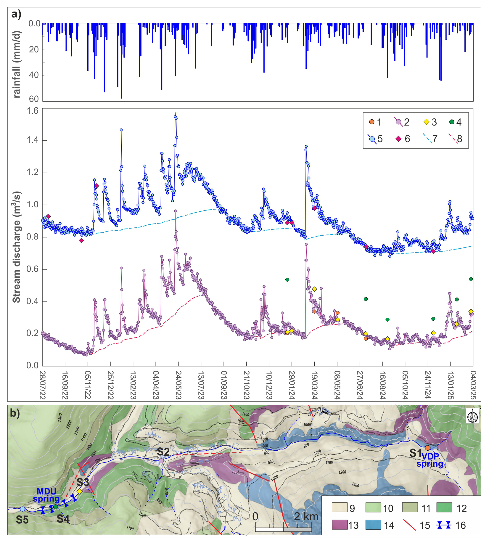
Figure 4 (a) Daily stream discharge data at stream gauges S2 and S5 with rainfalls recorded at Ussita gauge and base flow curves and the discrete monitoring carried out along the stream (1 – S1 section; 2 – S2 section; 3 – S3 section; 4 – S4 section; 5 – S5 section; 6 – discrete monitoring in S5 section; 7 – Base Flow at S5 section; 8 – Base Flow at S2 section). (b) location of stream sections on the geological map of Fig. 1a (9 – QUC; 10 – SCC; 11 – MFC; 12 – MAC; 13 – CSMC; 14 – BLC; 15 – Normal faults; 16 – Main GW inflows to the stream).

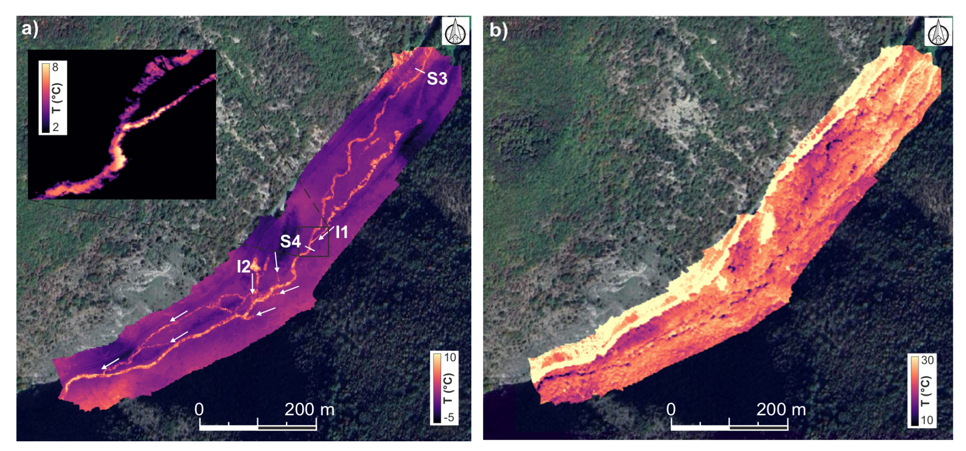
Figure 5 (a) Thermal drone investigations carried out in January 2024 and (b) in July 2025. Base map: map data © 2025 Google.

3 Results

3.1 GW-SW interactions along the stream

The integrated monitoring network of the Ussita catchment facilitated the understanding of factors influencing GW-SW interactions at multiple scales. Figure 4a displays continuous discharge data collected at stream gauges S2 and S5 (Fig. 1b), along with spot measurements from the OTT MF Pro at sections S1, S3, S4, and S5.

Moving from S1 to S3 (see Fig. 4b for the location of stream sections), the stream discharge during the no-recharge periods (e.g., stream discharge values are equal to baseflow) remains almost stable, indicating that the stream is mainly sustained by the VDP spring; thus, no significant GW inflows are present downstream of the spring up to Sect. S3. It should be noted that downstream of S3 towards S5, no tributaries that feed the Ussita stream are present. Based on mean discharge data from spot OTT MF Pro measurements acquired during the no-recharge periods (2022–2024), an initial increase in stream discharge due to GW inflow was registered between S3 and S4, estimated at about 200 L s⁻¹. Downstream of S4, during 2022–2024, a further mean discharge increase of about 450 L s⁻¹ was measured up to the closing section of the MDU catchment (section S5). Overall, between sections S3 and S5, a mean increase in discharge of about 650 L s⁻¹ is recorded. This evaluation was also confirmed by the discharge measurements conducted by tracer injection on 29 January 2024 (Fig. S2), at the beginning of a stream recession phase (Fig. 4a). Between S3 and S5, a stream discharge increase of about 695 L s⁻¹ was registered, a value close to the OTT MF Pro measurements (660 L s⁻¹) carried out during the tracer test, confirming the reliability of the streamflow measurement system.

Figure 5a also shows the base flow (BF) curves estimated for the S2 and S5 stream sections. According to Chapman (1991) and Tan et al. (2009), the filter parameter k was estimated by the recession constant derived from the MRC. The stream discharge data during the recession periods for both the S2 and S5 sections are fitted using the Maillet (1905) recession model, yielding α values of −0.0100 and −0.0033 d⁻¹, respectively. Then the k filters were set at 0.99 for the S2 section and 0.997 for the S5 section. The analysis of BF curves allowed the calculation of the BFI value in the two stream sections: it moved from about 0.80 in S2 to 0.90 in S5, highlighting the role of GW inflow along the stream stretch (S3–S5) in sustaining the stream discharge (Fig. 4a). The drone survey carried out in January 2024 has made it possible to identify stream stretches with groundwater inflows in the stream left and right banks (difficult to locate by just optical drone survey due to the shallow river). From Fig. 5a, it can be seen that water 1–2 °C warmer entered the main stream channel from I1 (left bank upstream of S4) and I2 (right bank downstream of S4), with additional diffuse GW inflow along the surveyed stream reach. The survey was repeated in July, but no relevant information was obtained due to dense vegetation along the river path (Fig. 5b). Instead, the absence of vegetation allows observation of the temperature contrast between groundwater and the surrounding land (including stream water).

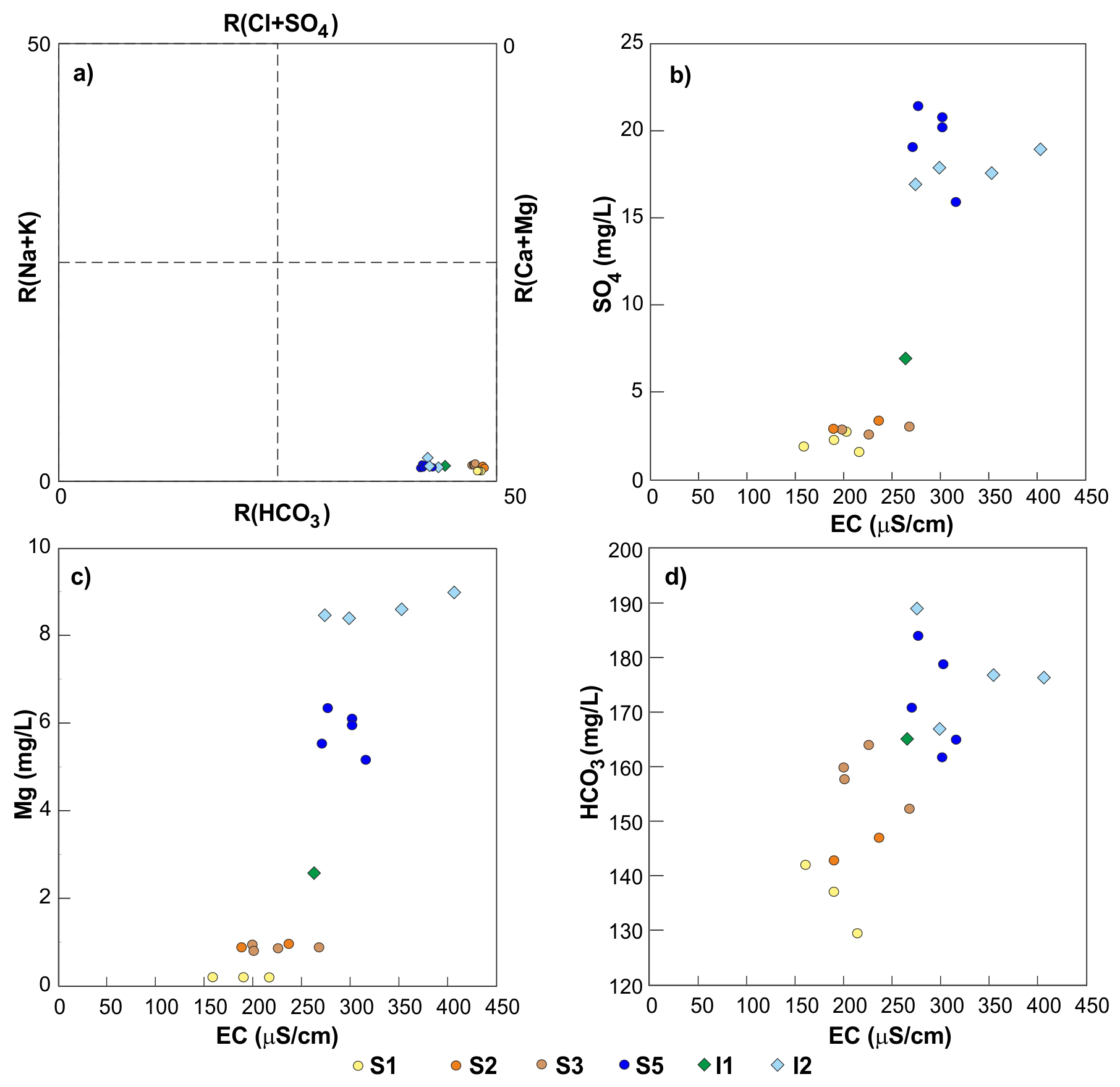
Figure 6 (a) Langelier-Ludwig diagram for the Ussita stream; (b) sulphate concentrations vs EC values; (c) Magnesium concentrations vs EC values; (d) Alkalinity vs EC values. For the location of sampling points, see Fig. 1.

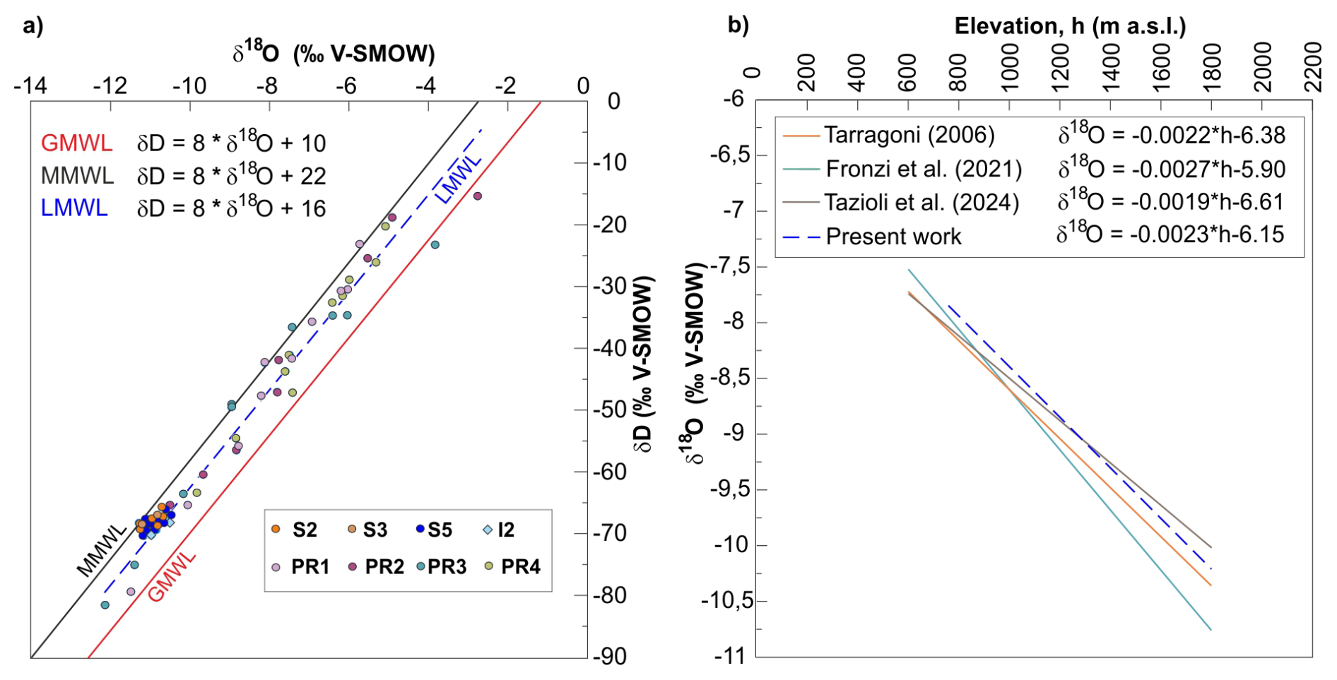
Figure 7 (a) δD vs δ¹⁸O values of precipitation samples with the resulting linear regression (Local Meteoric Water Line, LMWL), compared with the Global Meteoric Water Line (GMWL) and the Mediterranean Meteoric Water Line (MMWL); (b) Linear regression between δ¹⁸O and elevation determined by four water collectors (PR) with those proposed by Tarragoni (2006), Fronzi et al. (2021), and Tazioli et al. (2024). For the location of sampling points, see Fig. 1.

3.2 Hydrochemical and isotopic characterization of Ussita stream waters

The results of the systematic, approximately monthly campaigns from November 2023 to July 2024 for major soluble ions and other physical parameters (streamflow, temperature, pH, and electrical conductivity) are shown in Table S4. Regarding the stable water-isotope composition, Table S5 presents the δD and δ¹⁸O values of rain and stream waters sampled approximately monthly from June 2023 to March 2024. The analytical uncertainty of the chemical analyses for major soluble ions was evaluated using the Charge Balance Error (CBE), which ensures that the sum of all positive charges (cations) equals the sum of all negative charges (anions). For the data in Table S4, the average CBE is 2.8 %, which remains well within the commonly accepted ±5 % limit. For further details about the average and coefficient of variation of measures of each sampling point, refer to Table S6, for the major soluble ions, and to Table S7, for the stable water isotopes. Figure 6a shows the Langelier-Ludwig diagram for Ussita stream water, highlighting a bicarbonate-earth-alkaline composition typical of water interacting with carbonates, consistent with the lithological composition of the Ussita catchment (see Fig. 1). As shown in Figs. 6b,c, moving from site S1 to S5, the stream water's sulfate and magnesium contents increase (Fig. 6b, c), indicating two distinctly different hydrotypes. Specifically, there is a notable increase in sulfate and magnesium levels in the lower part of the stream (S5) compared to the upper sections (S1, S2, S3). Data reveal a more alkaline composition for S1, S2, and S3 stream water, whereas S5, along with I1 and I2, shows a less alkaline, slightly more sulfate-chloride composition (Fig. 6d).

Figure 7a displays the isotopic composition of water (i.e., δD and δ¹⁸O) at the sampling points, in relation to the Local Meteoric Water Line (LMWL), estimated from the isotopic composition of Ussita precipitation waters (PR1, PR2, PR3, and PR4 in Table S1), the Global Meteoric Water Line (GMWL; Craig, 1961), and the Mediterranean Meteoric Water Line (MMWL; Longinelli and Selmo, 2003). Figure 7a, as well as Table S5, show that overall, the precipitation values of δD and δ¹⁸O are more negative than those of stream waters. Moreover, precipitation values exhibit the highest CV values (from 35 % to 47 % for δD to 22 % to 35 % for δ¹⁸O) with respect to CV values in stream waters (from 1 % to 3 %), highlighting the strong effect of seasonality of precipitation water. Stream water samples show lc-excess values ranging from 0.41 ‰ to 6.04 ‰, with a standard deviation of 1.40 ‰ (see Table S4), and average and median lc-excess values are 2.75 ‰ and 2.74 ‰, respectively. Table S5 shows that, at each sampling point, the lc-excess average values range from 1.01 ‰ (I2) to 3.42 ‰ (S2), with relatively high CV values (38 %–84 %; Table S6). These generally positive lc-excess values indicate rapid infiltration of rainwater, which prevents isotopic fractionation typically caused by evapotranspiration processes, which are often associated with more negative lc-excess values (Sprenger et al., 2016). This supports the hypothesis of rapid and direct recharge of meteoric water into the groundwater system, as well as a significant contribution of groundwater to the baseflow of the Ussita stream.

Because this rapid infiltration minimizes fractionation and preserves the isotopic signature from precipitation (input) to stream discharge (output), once the δ¹⁸O – elevation relationship was established (see Fig. 7b, blue dashed line), this relationship was used to compute the Isotope Recharge Elevation (CIRE) values for the S1 and S5 sampling points, yielding elevations of 1855 m a.s.l. for S1 and 2193 m a.s.l. for S5.

These estimates were also compared with values derived from previously published δ¹⁸O-elevation relationships in the Mt. Sibillini area, specifically those reported by Tarragoni (2006), Fronzi et al. (2021), and Tazioli et al. (2024) (equations also shown in Fig. 7b). Based on all available relationships, the CIRE values ranged between 1672–1855 m a.s.l. for S1 and 1960–2193 m a.s.l. for S5.

3.3 Integrated approaches for computing the water budget and recharge area

The mean annual water budget was carried out over the MDU catchment (A=44 km²) using Eq. (3), referring to the 2019–2023 period. The unknown component $(Q_{\mathrm{in}}^{\mathrm{gw}}-Q_{\mathrm{out}}^{\mathrm{gw}}$) is considered a water-budget residual, and the Q $/$ WS ratio was calculated using the approach of Schaller and Fan (2009). All water budget components are presented in Mm³ yr⁻¹. The mean streamflow at S5, i.e., the catchment closure (Q), yields approximately 29.6 Mm³ yr⁻¹. The mean change in storage (ΔS), calculated by analyzing stream recession curves for each year and applying Korkmaz's (1990) Eq. (2), yielded a mean annual volume of about −0.964 Mm³ yr⁻¹. The following subsections report the results from the two water budget experiments (Case I and Case II), as detailed in Sect. 2.4.3. In both cases, the recharge area is estimated using Eq. (7).

3.3.1 Results of Case I

Table 2 shows the results of the Case I water budget (nineteen estimates). Within the uncertainties of the various water budget components, all the computations reveal that $Q_{\mathrm{in}}^{\mathrm{gw}}>Q_{\mathrm{out}}^{\mathrm{gw}}$, indicating that the potential extension of the hydrogeological catchment, computed by Eq. (7), is larger than the catchment one ($A^{*}=\mathrm{51.98}\pm \mathrm{4.08}$ km², compared to A=44.06 km²). The presence of groundwater inflow is also confirmed by the Q $/$ WS ratio, which exceeds 1 for all analyzed products, with a mean of about 1.22 (i.e., about 22 % of the Ussita stream discharge is fed by groundwater circulation from regions outside the catchment). In the computation of A^* values, an effective infiltration ($I=\mathrm{0.90}\times \mathrm{WS}$) over areas exceeding the catchment is considered (i.e., outside the catchment, about 10 % of WS contributes to the runoff towards other systems).

Table 2 Water budget results over the MDU catchment for the 2019–2023 period, using different ground-based, satellite, and reanalysis products to compute the water surplus (WS). A^* indicates the potential extension of the hydrogeological catchment.

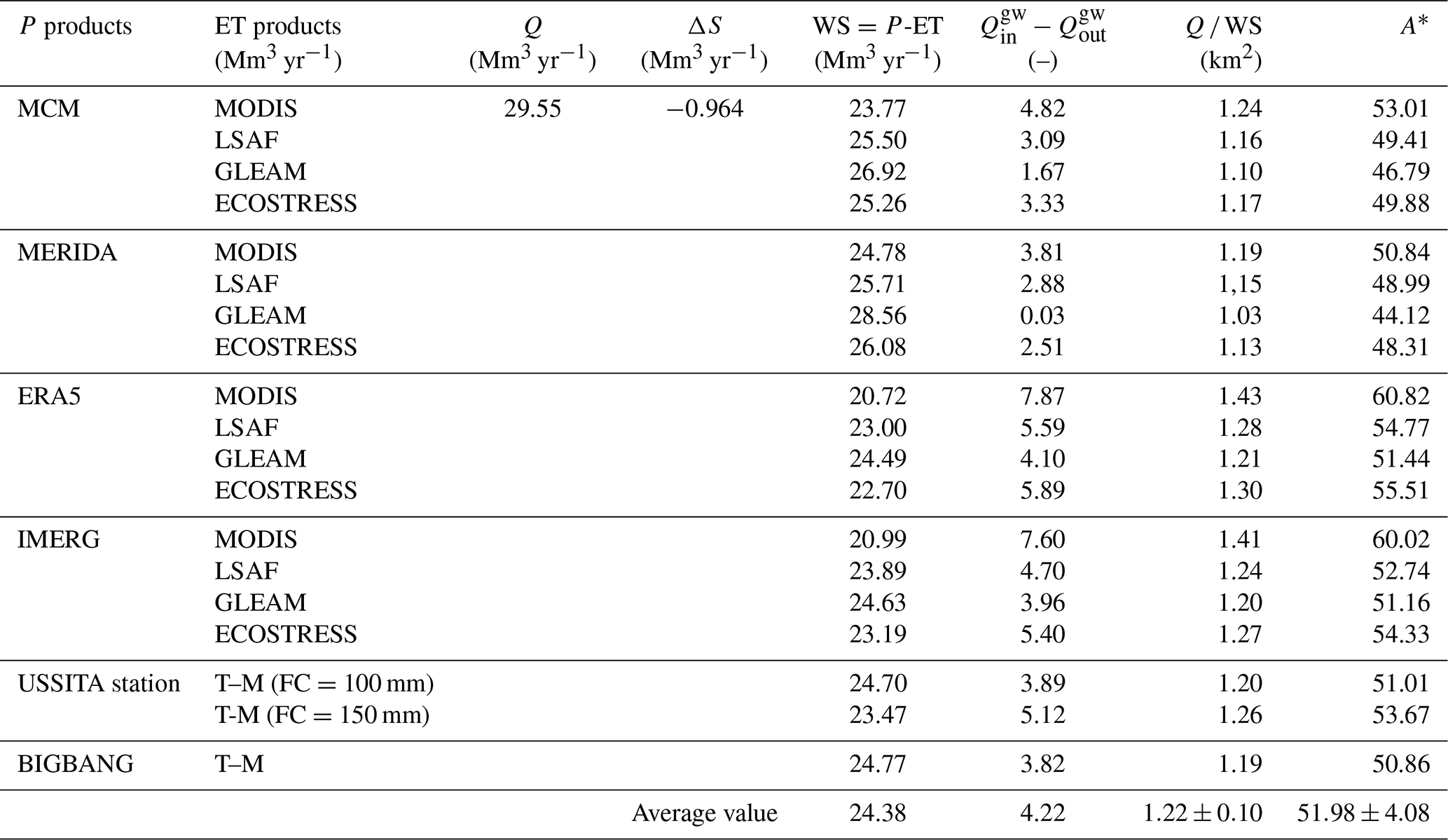
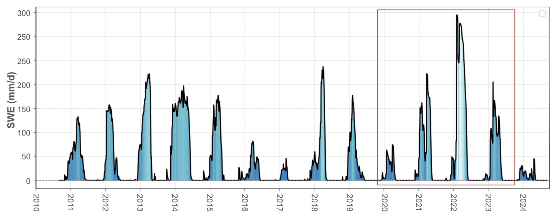
Figure 8 SWE values during the 2010–2024 period for the MDU catchment. The red rectangle represents the period used to compute the water budget.

It should be pointed out that among the P products in Table 2, the Ussita weather station and rainfall data used by the BIBGANG model refer to heated rain gauges, even if they are located at a very small altitude compared to the mean altitude of the MDU catchment; thus, they are not fully representative of the snowmelt contribution at the catchment scale (i.e., the mean altitude is 1315 a.s.l., with the stream headwater characterized by relief reaching an altitude higher than 2000 m a.s.l.).

3.3.2 Results of Case II: the role of snow melting in aquifer recharge

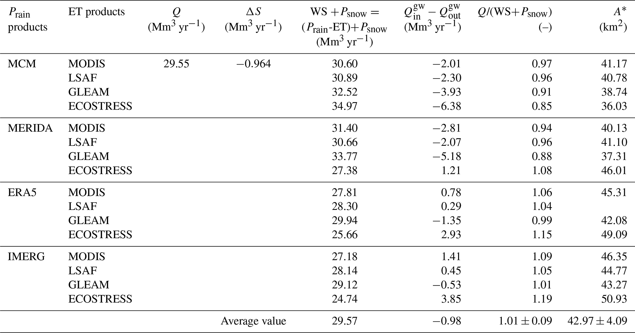
Table 3 shows the results of the Case II water budget. This case consists of sixteen different calculations of the water balance obtained by integrating the WS estimations based on P_rain as well as P_snow estimates based on SWE of IT SNOW, following the approach in Fig. 2. Figure 8 shows the mean daily IT SNOW SWE time series for the 2010–2024 period, highlighting a considerable contribution of snow, especially for the 2022 period. After integrating the snowmelt data (P_snow) into the WS values, it was possible to recompute the water budget, with the results summarized in Table 3. Considering the contribution of snowmelt, the average hydrogeological catchment was 42.97±4.09 km², practically similar to the catchment area. It indicates that GW inflows ($Q_{\mathrm{in}}^{\mathrm{gw}}$) are negligible, highlighting the important role of snowmelt in the catchment.

Table 3 Water budget results over MDU catchments using different ground-based, satellite, and reanalysis products to compute the water surplus (WS), integrated with P_snow derived from the IT SNOW dataset. A^* indicates the potential extension of the recharge area.

4 Discussion

4.1 Integrated approaches to improve understanding of groundwater-surface water interactions

We investigated the processes that control the spatial and temporal dynamics of groundwater–surface water (GW–SW) interactions in a mountainous sector of the Central Apennines by combining ground-based monitoring with remote sensing. As noted by Ma et al. (2024), applying such methods in specific regional contexts is essential for understanding the spatial scales at which they are valid and their respective strengths and limitations. This knowledge is critical for building a reliable and comprehensive picture of the hydrogeological systems that sustain mountain streams. Thanks to the integrated approach, we captured the spatial-temporal dynamics of groundwater–surface water interactions. Gaining stream is one possible scenario of GW-SW interactions (Irvine et al., 2024), which depend strongly on the spatial scale at which they occur. In this study, we employed a suite of complementary techniques – including differential stream gauging, physical hydrograph separation, surface-water tracer tests, and thermal and optical UAV surveys – that align with the best-practice methods identified in the GW/SW Method Selection Tool (GW/SW-MST) developed by Hammett et al. (2022). In mountain regions, acquiring basic data through complementary techniques provides insights into the hydrogeological system, making it a best practice to optimize the cost-benefit ratio and achieve the best possible results, given the multiple factors involved in complex environmental systems (e.g., Samani and Moghaddam, 2022). In detail, the main advantage of the integrated approach is the investigation of the spatial distribution of GW inflow along the Ussita stream, revealing that most of the baseflow in the stream from S1 to S3 is sustained by the VDP spring (Q≃220 L s⁻¹), with a huge baseflow increase between S3 and S5 sections (Q≃650 L s⁻¹) delineating, two different sources of alimentation: (i) the Maiolica Complex for the VDP spring (EC ≃210 µS cm⁻¹; SO₄≃2.5 mg L⁻¹), and (ii) the Base Limestone Complex for punctual and linear springs downstream of the S3 section and up to S5 (EC ≃310 µS cm⁻¹; SO₄≃18.7 mg L⁻¹), with some mixing water with intermediate characteristics in the I1 sampling point related to the Maiolica Complex contribution (Ussita left bank, Fig. 1, EC ≃264 µS cm⁻¹; SO₄≃6.9 mg L⁻¹). It should be noted that the continuous stream discharge in S2 and S5 allows for capturing short-term stream transient dynamics and checking the results of BF separation estimations, while the spot discharge measurements in sections S1, S3, and S4, although they are not numerous, are useful to roughly quantify the BF during the no-recharge periods. Although groundwater inflow points and stream stretches were identified by a single drone survey in the winter of 2024, the analysis can be considered reliable because it was conducted during a no-recharge period (e.g., Fig. 4a) and under hydrometeorological conditions favorable for highlighting GW–SW water temperature contrasts, the latter not possible during the summer of 2024 due to the high vegetation cover and small temperature contrasts between GW and SW. Overall, the findings highlights that in the lowest part of the MDU catchment (downstream of S3 up to S5, Fig. 1) the GW circulation feeding the basal linear and punctual springs show clear signs of interactions with low-permeability anhydrites (CaSO₄) and dolomites (CaMg(CO₃)₂) of the Evaporites Complex underlying the Base Limestone Complex, outcropping in a small tectonic window in the stream's right bank (less than 1 km north to S3 section, see Fig. 4b). This figure confirms that the geological features of the catchment control the hydro-geochemical characteristics of the baseflow (e.g., Farvolden, 1963; Winter, 2001; Bloomfield et al., 2009; Segura et al., 2019). As reported by Levin et al. (2023), measurements made at a point or field scale are not easily extrapolatable to a catchment scale because of the spatial heterogeneity of preferential flow paths.

4.2 Estimation of the recharge area

We carried out a multi-source annual-average water budget (e.g., Vargas Godoy et al., 2024) using the most detailed datasets available for the study area, with the highest spatial and temporal resolutions. Among the products we used, IT-SNOW, MCM, and ECOSTRESS (Table 1) have spatial resolutions (ranging from 70 m to 1 km) that can be suitable for analyzing hydrological processes in mountain watershed areas (e.g., Shuai et al., 2022). Although the delineation of the recharge area feeding the basal linear and punctual springs of the Ussita stream remains challenging, the results from the water budget allowed, by using different ground-based, satellite, and re-analysis datasets, to define and constrain its extension (i.e., the area of the hydrogeological basin is close to the catchment one). This finding is confirmed by the isotope data and analysis of CIRE, which indicates recharge elevations of up to 2193 m a.s.l. for the MDU system (at Sect. S5) and 1855 m a.s.l. for the VDP spring (at Sect. S1). These values are consistent with the catchment's topographic configuration and hydrogeological setting, confirming that the main recharge occurs in the highest parts of the catchment, above 2000 m a.s.l., where snow accumulation and subsequent melt are most significant. The isotopic composition of stream water (δ¹⁸O and δD), coupled with generally positive lc-excess values (mean =1.76 ‰), highlights rapid infiltration with minimal evaporative enrichment, supporting the hypothesis of direct recharge by meteoric waters. The δ¹⁸O further supports the spatial pattern of recharge-elevation regression line, which matches previous studies in the area (Tarragoni, 2006; Fronzi et al., 2021; Tazioli et al., 2024), confirming the robustness of this approach in mountainous carbonate contexts.

Additionally, the recharge elevations inferred from CIRE align well with the hydrochemical shift observed between S3 and S5, where a marked increase in sulphate and magnesium concentrations reflects the influence of deeper groundwater flow paths interacting with the Evaporites Complex. The isotopic evidence allows us to constrain both the origin and the altitude of recharge areas, providing independent validation of the hydrological processes inferred from water budget and hydrochemical results. The delineation of the recharge area for both the MDU and VDP sectors is further corroborated by multiple dye tracer tests conducted in the region by several authors (Nanni et al., 2020; Fronzi et al., 2020, 2021; Cambi et al., 2022; Mammoliti et al., 2022). These studies, based on six artificial tracer tests, revealed no evidence of groundwater input from outside the Ussita catchment's hydrological boundaries, reinforcing the hypothesis of a predominantly internal recharge regime. The evaluation of the recharge area is a key aspect for mountain regions, considering that using rain gauges alone is particularly problematic because they are systematically installed at lower elevations and are not representative of high-elevation precipitation and heterogeneous snowfall patterns (Cambi et al., 2010; Daly et al., 2017; Ly et al., 2013; Di Matteo et al., 2017).

Overall, the GW contribution in the MDU system (i.e., the average baseflow given as specific discharge, q) was estimated to be about 22 L s⁻¹ km⁻², a value falling in the range of 18–24 L s⁻¹ km⁻², as obtained by Boni et al. (1986) for rivers fed by carbonate aquifers in the mountain ridge of Central Italy. Integrating the precipitation range in the area derived from the different estimations (mean value of about 1000 mm yr⁻¹), the specific discharge of the Ussita catchment falls in the class III (humid areas) based on the global distribution of carbonate rocks and karst water resources (Goldscheider et al., 2020).

4.3 Importance of snow for aquifer recharge

The contribution of snowmelt to the water budget in mountainous regions remains poorly understood and is difficult to evaluate due to the scarcity of ground-based observation networks. As inferred from the MDU catchment, snowmelt contributes significantly to aquifer recharge, accounting for about 18 %. This value aligns with recent evaluations conducted on other hydrogeological systems of the Central Apennines. Lorenzi et al. (2023), based on satellite images of snow cover from 2019 to 2022 over the Gran Sasso aquifer, found that snowmelt contributed roughly 15 % of the total aquifer recharge, highlighting the importance of snow-covered periods in areas characterized by karst features. Recently, Rusi and Di Giovanni (2024) collected six years of ground-based rainfall and snow-cover data from 2018 to 2023 for six carbonate aquifers in Central Italy, spanning the Gran Sasso to Monte Marsicano. Their analysis, using data from seven snow-cover measurement stations, revealed that snowmelt contributed between 10 % and 30 % of total infiltration. Overall, our study emphasizes the good performance of the IT-SNOW datasets in evaluating snowmelt contributions to aquifer recharge in Italian mountain regions. This finding is particularly important given that, over the past decade, snow cover thickness – including in the highest parts of the MDU catchment – has been very low in some years (2016, 2017, 2020, and 2024, Fig. 8). In this context, the observed percentages of aquifer recharge from snowmelt for the MDU catchment and other hydrogeological systems in Central Italy and elsewhere can help address the ongoing question regarding the connection between snowmelt and groundwater flow in snow-dominated regions of the Mediterranean area (e.g., Fayad et al., 2017).

4.4 Water budget components uncertainty: possible future directions

Characterizing uncertainty in water budget components, including Earth Observation datasets, is complex, especially in small mountain catchments (Levin et al., 2023; Marti et al., 2023). Generally, the water budget equation includes a residual term (Res), which sums the potential inaccuracies of the datasets used in the calculation (Res_i) and the omitted components in the original equation (Res_o). Most studies simplify water budget uncertainty analyses by neglecting a priori certain components, such as assuming no net groundwater exchange $(Q_{\mathrm{in}}^{\mathrm{gw}}-Q_{\mathrm{out}}^{\mathrm{gw}}=\mathrm{0}$); e.g., Yoon et al. (2019) and Barbosa et al. (2022). As reported by Genereux et al. (2002), intercatchment groundwater flows (included in Res_o) cannot be directly measured and are therefore difficult to quantify, which can explain why they are often overlooked in catchment studies. In this way, the entire water imbalance error (Res) is often fully redistributed across budget components, leading to contradictory results such as a decline in the accuracy of corrected hydrological datasets (Luo et al., 2023).

Recently, Zheng et al. (2025) provided a comprehensive list of methods to reduce the impact of data inconsistency for improving water budget closure, such as the constrained ensemble Kalman filter (CEnKF, Pan and Wood, 2006), the multiple collocation (MCL), and proportional redistribution (PR) methods (Abolafia-Rosenzweig et al., 2020; Abhishek et al., 2022; Luo et al., 2023), as well as the post-processing filtering technique (PF) and bias correction method (Munier et al., 2014; Weligamage et al., 2023). It should be noted, as Abolafia-Rosenzweig et al. (2020) pointed out, that the potential incorrect assignment of residuals results from the closure constraints and assumptions imposed by the methods mentioned above. Zheng et al. (2025) proposed a more advanced approach to quantify Res_o by modelling 653 catchments in the USA, which have much larger areas than the Ussita catchment, covering only 44 km². As reported by Muñoz et al. (2024), the use of more sophisticated approaches to evaluate uncertainties in water management in mountain regions requires probability distributions, which can be difficult to obtain in data-scarce regions. Bouaziz et al. (2018) examining the water budget in 58 small limestone fractured/karst catchments along the Meuse River at the border between France and Belgium, concluded that, due to the nature and complexity of the catchments, net groundwater exchanges are the primary cause of water balance discrepancies, which are most significant in small catchments, consistent with the earlier findings of Schaller and Fan (2009). Although evaluating water budget uncertainties is beyond the scope of our study, the multi-source water budget we conducted (35 combinations, 16 of which included the snowmelt contribution) identified groundwater exchanges as the main residual, as reported by Bouaziz et al. (2018). We recognize that more advanced methods for accounting for uncertainty in water budget components could further enhance quantification and refine the assumptions (e.g., by considering the propagation of uncertainty of products reported in the Sect. S1), even if the results from the multi-source water budget align with those from tracer tests (Nanni et al., 2020; Fronzi et al., 2020; Fronzi et al., 2021; Cambi et al., 2022; Mammoliti et al., 2022).

4.5 Modelling approach perspectives

The experimental evidence derived from our integrated, multi-disciplinary approach provides a basis for formulating conceptual hypotheses about the functioning of the groundwater system feeding the Ussita stream. Such hypotheses are a fundamental prerequisite for designing a conceptual model that supports the development of numerical and analytical groundwater models (e.g., Anderson et al., 2015). As reported by Enemark et al. (2019), traditionally, a single conceptual model serves as the basis for model predictions, even if the available data on the groundwater system support more than one conceptualization. Multi-model or flexible-structure approaches offer promising tools for testing an ensemble of conceptual understandings consistent with prior knowledge and observational data (e.g., Rojas et al., 2010; Kavetski and Fenicia, 2011; Mustafa et al., 2020). Refsgaard et al. (2006) reported that the modelling approach may involve a step-by-step procedure that defines a protocol for assessing conceptual model uncertainty. Our data and groundwater hypotheses can help future modelling approaches to define and refine the model structure. In this framework, the analysis of the recharge area extent that we conducted using a multi-source approach can support the definition of boundary conditions and help the model calibration. In detail, the PTV thrust and the outcrop of the Marne a Fucoidi hydrogeological complex (Fig. 1) constitute the no-flow boundaries that support the definition of the initial model domain, while the stream stretches fed by groundwater represent the constant-head boundaries where the baseflow represents the main component of streamflow (e.g., Staudinger et al., 2019). Moreover, streamflow data from the two stream sections (S2 and S5) are invaluable for calibrating and validating numerical models, especially in complex mountain environments; thus, data collection and experimental design represent a substantial field effort and play a pivotal role in reducing uncertainty and constraining future model simulations.

5 Conclusions

This study, conducted in the Ussita catchment (Central Apennines), demonstrates that an integrated, multi-disciplinary approach is required to understand groundwater (GW)–surface water (SW) interactions in fractured carbonate mountain regions. By combining hydrochemical and isotopic tracers, thermal drone surveys, and discharge monitoring, we were able to (i) distinguish among water sources and (ii) map spatially distributed zones of groundwater inflow to the stream, including reaches that are difficult to detect using standard field observations due to dense riparian vegetation.

The results highlight strong lithological controls on GW contributions to streamflow. Aquifers hosted in the Maiolica Complex (MAC) feed the VDP spring in the headwaters and largely sustain discharge in the Ussita Village catchment, where baseflow dominates streamflow (BFI ≈80 %). Conversely, downstream towards the catchment outlet (Madonna dell'Uccelletto catchment, MDU), the role of the Basal Limestone Complex (BLC) becomes dominant, and the BFI increases to ≈90 %. These findings are particularly relevant in tectonically complex carbonate systems, where preferential flow paths and gaining reaches are difficult to identify and quantify.

Integrating in situ monitoring with satellite-based products also enabled, within the uncertainties of some components of the water budget, tighter constraints on water-budget closure and recharge area extent, explicitly accounting for contributions from both rainfall and snowmelt. The multi-source water-budget analysis indicates that snowmelt contributed ∼18 % of aquifer recharge during 2019–2023. This result suggests that future reductions in snowpack accumulation and meltwater release may significantly reduce groundwater availability and, consequently, dry-season stream discharge, with implications for ecosystem functioning and water-supply reliability.

Although the hydrogeological functioning of carbonate mountain catchments remains site-specific, the integrated workflow proposed here is transferable and can guide field campaigns in similar data-scarce Mediterranean catchments, supporting the identification of the dominant controls on GW inflows to streams and the delineation of recharge areas.