Water flow timing, quantity, and sources in a fractured high mountain permafrost rock wall

Water flow in high mountain rock walls is crucial for landscape evolution and slope stability. However, the timing, quantity, and sources of this flow remain poorly understood. In the Mont Blanc massif, tunnels at the Aiguille du Midi peak (3842 m) provide direct access to steep permafrost-affected rock walls. Between May 2022 and October 2023, we monitored water flowing from fractures using a real-time system that measured flow rate, temperature, electrical conductivity, and fluorescence of tracers, alongside meteorological data and ground surface temperatures.

The results indicate high surface–subsurface connectivity. The water source is primarily snowmelt, with additional inputs from late-summer rainfall. Electrical conductivity, stable isotopes, and recession curve analysis suggest another source of older subsurface ice. Flow onset was closely tied to air temperatures, with steady diurnal fluctuations appearing once rock surface temperatures exceeded 0 °C. Lag times between daily peaks of flow rate and peaks of air and ground surface temperatures of 3–9 and 0–3 h, respectively, point to rapid unsaturated infiltration conditions. Distinct flow regimes observed in two adjacent fracture systems reflect a complex, heterogeneous network, including sediment-filled fractures with a delayed response. Significant flow rates (often > 10 L h⁻¹) and water temperature often exceeding 5 °C, suggest significant heat transfer by advection, capable of enhancing permafrost degradation.

This study provides rare direct observations of fracture flow dynamics in steep permafrost rocks and improves our understanding of water routing and its response to atmospheric forcing. The findings offer valuable constraints for coupled hydrothermal models, permafrost-related hazard assessments, and the potential impact of climate change.

1 Introduction

1.1 Hydrogeology of high mountains

Water plays a crucial role in weathering and erosion processes in mountainous landscapes. In the periglacial belt, the presence of water in the shallow subsurface can cause rock fracturing through ice segregation or volumetric expansion, depending on temperature conditions and saturation levels (Draebing and Krautblatter, 2019; Matsuoka and Murton, 2008). Hydrostatic pressure in undrained fractures can drive catastrophic failure (Hasler et al., 2012; Krautblatter et al., 2013; Scandroglio et al., 2021; Walter et al., 2020). Over geological time scales water is a key catalyst of mechanical rock weathering processes related to subcritical cracking (Eppes and Keanini, 2017). The melting of ice in joints under thawing conditions can release detached blocks and lead to debris and rock falls, and the formation of scree slopes (Hales and Roering, 2007). Water infiltration in bedrock may also trigger large rock slope failures by reducing the friction of rough fracture contact surfaces (Krautblatter et al., 2013). In permafrost ground, the presence of sealing ice in pores and fractures favors the development of high hydrostatic pressures (Fischer et al., 2010; Marcer et al., 2020), which may increase the frequency or magnitude of mass movements. In addition to mechanical pressure, water circulation can also cause thermal perturbations with potential cooling effects in some cases (Maréchal et al., 1999; Phillips et al., 2016) or warming effects in others (Hasler et al., 2011; Phillips et al., 2016). In permafrost ground, heat advection from water infiltration could accelerate permafrost degradation (Gruber and Haeberli, 2007; Hasler et al., 2011; Magnin and Josnin, 2021), and potentially develop thawing corridors (Krautblatter and Hauck, 2007; Keushing et al., 2017). Recent observations of increased rock fall activity in high mountains regions have been linked to permafrost degradation (Allen et al., 2009; Fey et al., 2025; Gruber et al., 2004; Huggel et al., 2012; Legay et al., 2021; Ravanel et al., 2017; Ravanel and Deline, 2011). The warming of intact frozen rock is commonly related to rockwall destabilization due to a decrease in rock uniaxial and tensile strength (Dwivedi et al., 1998; Krautblatter et al., 2013; Li et al., 2003; Mellor, 1973). Water-related processes have been suggested as a potential cause of several rock fall events (Cathala et al., 2024; Erismann and Abele, 2001; Scandroglio et al., 2021; Strauhal et al., 2016). However, while hydrogeological studies in alpine permafrost have primarily focused on coarse-grained terrain, such as rock glaciers (Bast et al., 2024) and scree slopes (Pellet and Hauck, 2017), little is known about water dynamics within bedrock rockwalls – despite their critical role in slope stability and landscape evolution.

1.2 Existing knowledge on water flow and infiltration in mountain permafrost

In steep alpine bedrock, the question of water infiltration and its thermal and mechanical implications is crucial but is rarely addressed directly (Krautblatter et al., 2013). Studying hydrogeological processes in these environments poses several challenges, including limited accessibility, the hidden nature of water flow pathways, strong spatial and temporal variability, non-linear system behavior, and the difficulty of identifying water sources quantitatively. Hasler et al. (2011) used numerical simulations to explore the impact of advective heat transport by water percolation on subsurface temperatures and ice-level changes. In the absence of hydrogeological field measurements, they performed laboratory experiments and demonstrated significant implications for the role of water flow in thaw-related instabilities in cold mountain permafrost regions. Maréchal et al. (1999) used a hydrothermal model to simulate an observed thermal anomaly that was found during drilling work in the road tunnel under the Mont-Blanc massif and showed that infiltration of water from the surface contributed to the continuous cooling of the alpine massif at depth. Ben-Asher et al. (2023) estimated the potential water input in steep alpine bedrock using field measurements and numerical simulations.

Apart from indirect studies (Ben-Asher et al., 2023; Hasler et al., 2011; Maréchal et al., 1999; Scherler et al., 2010), few studies have attempted to directly monitor groundwater flow in steep, permafrost-affected alpine environments (Gabrielli et al., 2012; Manning and Caine, 2007). In a recent study, Scandroglio et al. (2025) measured water outflow in 55 m deep fractures under the permafrost-affected Zugspitze Ridge (2815–2962 m a.s.l.). They compared their dataset with meteorological data and a snowmelt model to infer the timing and quantity of water flow and constrain the hydrological pressure in the fractures. They also analyzed recession curves of the measured flow rate, a technique that was never applied to alpine rock fractures before.

1.3 Saturated and non-saturated flow

From a hydrogeological perspective, a fractured summit is more accurately described as a permeable infiltration zone than as an aquifer. However, due to the scarcity of drilling data, constraints on the thickness of the high-elevation alpine unsaturated zone remain highly limited (Maréchal, 1998). The first tests of hydrodynamical models of a high alpine and permafrost-affected rock wall site were performed by Magnin and Josnin (2021) on the Aiguille du Midi site. This study showed that the unsaturated zone is probably more than 1000 m thick.

Generally, unsaturated conditions apply in soils, permeable rocks, and deposits, and water flow is often considered subvertical and evaluated using the Richards equation (Smith, 2002). In crystalline rock settings, porosity and permeability are essentially controlled by the geometry of the fracture network, where most of the water flow occurs. The water flow in fractures is thus not uniform but occurs along preferential flow paths sometimes called “fingers” (Su et al., 2000), that channel the flow path at the larger scale of the fractured medium (Tsang et al., 2013). These preferential flow paths have been observed in both saturated and unsaturated fractures (Su et al., 2000).

In the study area of the Mont-Blanc massif, the fracture network opening is highly irregular (from millimeters to decimeters, depending on the fractures) and is expected to evolve seasonally, with reversible opening in winter (Guillet et al., 2018), superimposed on an irreversible long-term opening trend (Weber et al., 2017). The fractures can also be affected by the water flow, which can change the extent of ice filling or plugging and develop partially saturated conditions similar to those known from some epikarsts (Ford and Williams, 1989).

The objective of this work is to quantify the timing, quantity, and sources of water flow within this fractured permafrost rock wall, and to evaluate how flow dynamics are influenced by atmospheric forcing and surface conditions. Specifically, we aim to (1) characterize seasonal and diurnal variability in fracture flow, (2) assess the relative contribution of different water sources, and (3) examine the coupling between thermal conditions and hydrological response.

In the next sections, we first introduce the study area and monitoring approach and then describe the data and analytical methods. We then present the main hydrological and thermal observations and examine their implications for water flow processes in fractured permafrost rock walls. The paper concludes with a synthesis of the key findings and their broader significance.

2 Study site and meteorological context

2.1 Aiguille du Midi site

The Aiguille du Midi (AdM) is a peak composed of three granite pillars - Piton Nord, Piton Central, and Piton Sud. The central pillar (Piton Central) reaches an elevation of 3842 m a.s.l. and towers approximately 3000 m above the valley of Chamonix (Fig. 1). The site lies on the NW flank of the Mont Blanc massif (MBM) which covers an area of about 550 km² and is oriented NW-SE between France, Italy, and Switzerland.

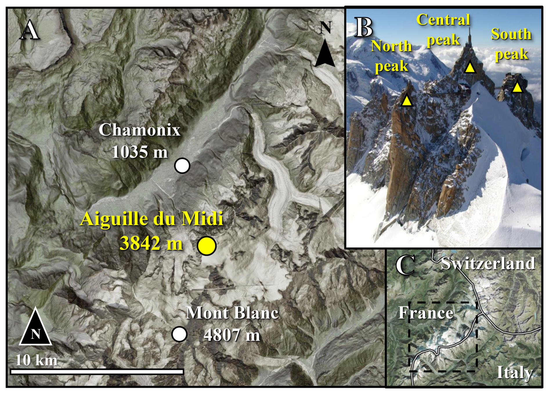
Figure 1 (A) Location of the Aiguille du Midi in the Mont Blanc massif. (B) view of the three peaks at Aiguille du Midi (Picture: S. Gruber). (C) Location of the Mont Blanc massif on the border of France, Italy and Switzerland. Maps provided by the Swiss Federal Office of Topography swisstopo.

Glaciers occupied about 100 km² in the late 2000s (Gardent et al., 2014) while permafrost is largely present above approximately 2600 m in N faces and 3200 m in S faces (Magnin et al., 2015a).

The combination of steepness, permafrost, and glacial dynamics results in highly active morphodynamics (Deline et al., 2015). Over the past decades, rockfall (volume > 100 m³) frequency has significantly increased (Ravanel and Deline, 2011), notably during the hot summers. The main cause has been suggested to be permafrost degradation (Ravanel et al., 2017; Legay et al., 2021; Magnin et al., 2023). Permafrost investigation started in the mid-2000s in the MBM, with the installation of various temperature sensors in AdM (Magnin et al., 2015b), including 10 m deep boreholes, which recorded a temperature increase of over 1 °C during the 2011–2020 decade (Magnin et al., 2024).

AdM has been chosen as a pilot site for alpine permafrost investigations because of its representativeness of high alpine rockwalls and its accessibility from Chamonix by a cable-car. Man-made tunnels, terraces, bridges, and an elevator allow the visitors to access different parts of the site. Since the hot summer of 2015, water flowing from the fractured tunnel walls has become a problem for the operating company (the Compagnie du Mont Blanc), leading to the installation of a drained metal plate ceiling to divert the flowing water and keep some parts of the tunnels dry for visitors.

2.2 Meteorological conditions in 2022 and 2023

As of 2024, in Europe, the years 2022 and 2023 were the third and second warmest years in record after 2020, respectively, with a mean annual air temperature (MAAT) about 1.1 °C above the 1991–2020 average (Copernicus Climate Change Service, 2023, 2024). Summer 2022 was the warmest summer ever recorded, outpacing the 1991–2020 average by 1.4 °C (Copernicus Climate Change Service, 2023). September 2023 was the warmest September on record (Copernicus Climate Change Service, 2023).

Air temperature (AT) and precipitation records in the town of Chamonix (France), located in the valley just north of AdM (Fig. 1), began in the early 20th century and are well-suited to characterize the local precipitation regime. At AdM, AT records started in 2007 but are affected by numerous gaps that sometimes last several months, making this data less reliable for multi-annual comparison.

Figure 2 shows AT and precipitation in Chamonix and at AdM for 2022–2023. Winter and early spring 2022 were markedly warmer and drier than in 2023, with mean AT at AdM about 1.4 °C higher and precipitation roughly half as much. A late-spring heat wave produced a record high AT in May 2022, while May 2023 was near average. Summer conditions were generally warmer in 2022, but an exceptional late-season heat wave occurred in September 2023, the warmest on record in Chamonix, whereas September 2022 was near normal. Overall, 2023 was wetter than 2022, mainly due to higher precipitation in spring and autumn.

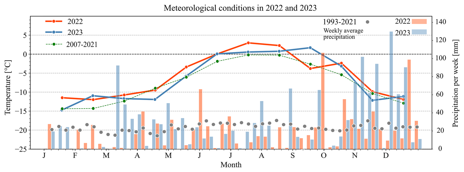
Figure 2 Monthly average air temperatures (lines) and weekly precipitation (bars) in 2022 (orange) and 2023 (blue). Air temperature was measured at the site in Aiguille du Midi (3842 m a.s.l.). Precipitation was measured in Chamonix (1042 m a.s.l.), since no reliable precipitation data is available at the high elevation site. Data provided by Météo France. The long-term average air temperature (2007–2021) is presented as a green thin dashed line. The long-term average weekly precipitation in Chamonix (1993–2021) is shown by gray circles.

In summary, 2022 was characterized by a very early but long-lasting and record-breaking summer heat wave, while 2023 was characterized by a late and record-breaking summer heat wave with significantly more precipitation than in 2022.

3 Methods

In April and May 2022, we installed a monitoring system to measure characteristics of water flowing through fractures in the roof of the tunnel in AdM (Figs. 3, 4).

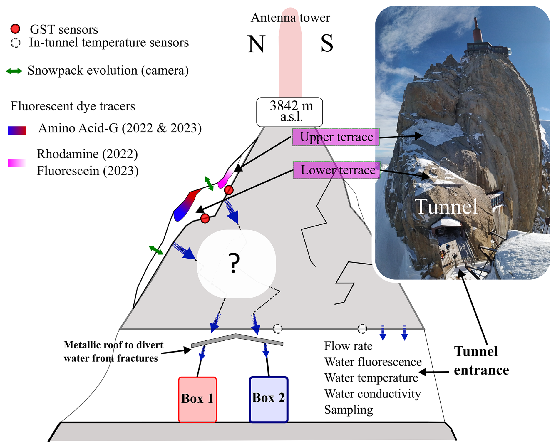
Figure 3 Sketch of the methodological approach to track and monitor water flows in the Aiguille du Midi central pillar. Note the location of the dye tracers in the snowpacks on the terraces above the water monitoring boxes.

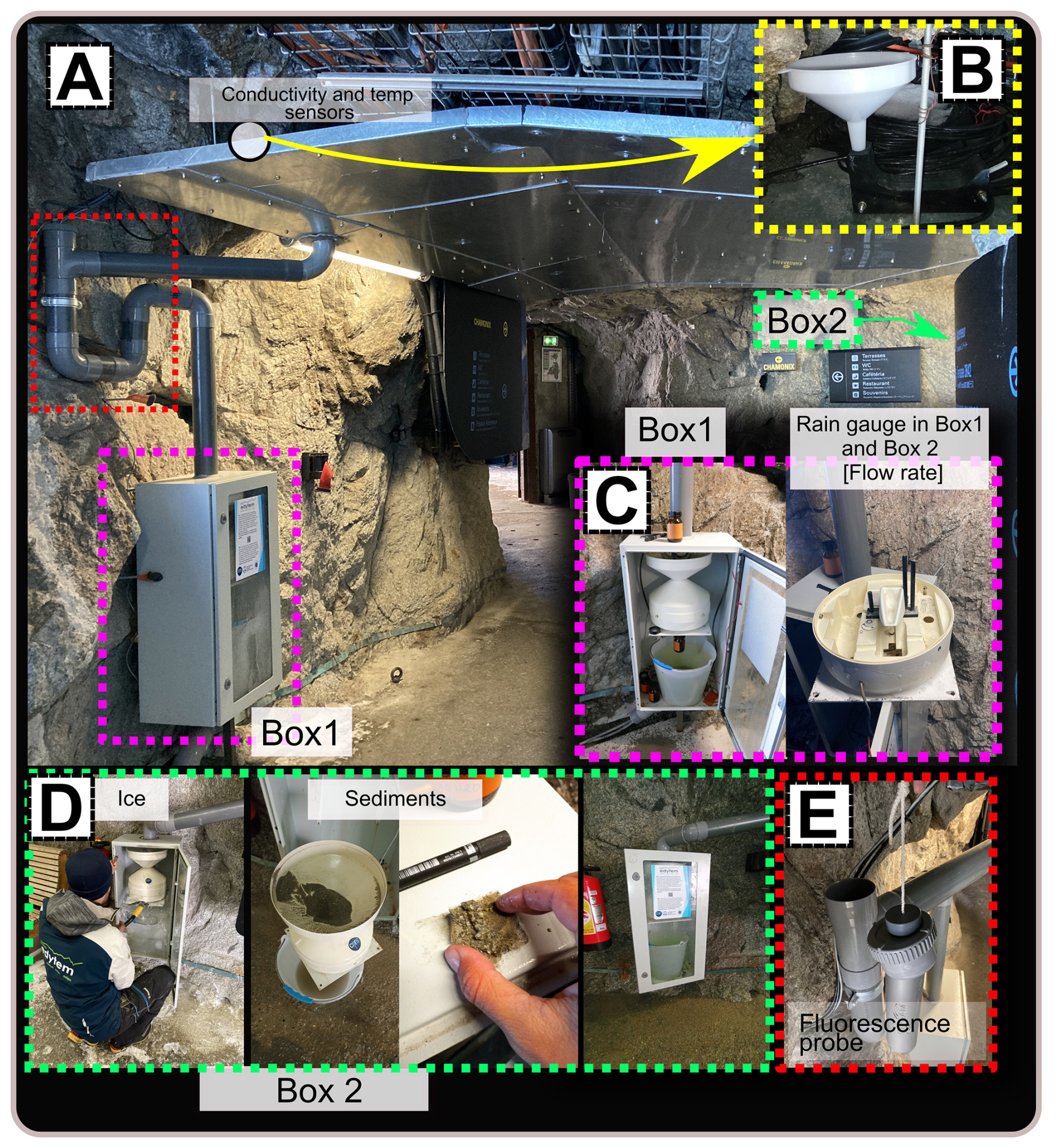
Figure 4 Real-time monitoring system in the tunnel. (A) The metal roof and Box 1 (pink dashed frame). (B) A 3D printed siphon that was placed directly under the water output from the fracture, equipped with temperature and conductivity sensors (yellow dashed frame). (C) Box 1 interior with rain gauge to monitor flow rate, a sampling bottle, and a bucket. (D) Box 2 with sediments (green dashed frame). (E) Fluorescence probe by TRAQUA located in a specially designed siphon for continuous real-time monitoring of the dye tracers.

3.1 Fluorescent dyes in the snowpack

Fluorescent dyes were inserted into the snowpack at the surface above the tunnel in two locations, directly above the fractures (Fig. 3), to trace the water source and rate of infiltration. In the 2022 season, two dye solutions were used: 20 L of sulphorhodamine-B (SRB) solution with a concentration of 0.001 g L⁻¹ and 20 L of amino acid G (AAG) with a concentration of 20 g L⁻¹. These solutions were prepared and carried in “Ondine^®” mineral water bottles by inserting the dye powders directly into the original mineral water, each with a volume of 5 L. The relatively low concentration of SRB was chosen to have a light but detectable pink color, far above the detection limit of the fluorimeter sensor.

In 2023, new solutions were prepared in the same manner, using 1.5 L bottles of “Ondine^®” mineral water. SRB was replaced by fluorescein dye (FLC), a much more soluble and detectable dye, to avoid confusion with SRB from the previous year. In total, 9 L of FLC solution with a concentration of 0.667 g L⁻¹ and 16 L of AAG solution with a concentration of 12.5 g L⁻¹ were prepared.

In both years of the study, tracers were injected into the snowpack at the same two locations on the north face of the central peak (Fig. 3). SRB in 2022 and FLC in 2023 were injected on the “upper” terrace of the face, which is located 18–24 m above the tunnel, while AAG was injected on the “lower” terrace, 7–12 m above the tunnel, in 2022 and 2023. The tracers were inserted in spring, before the flow started: on 11 May 2022 and 22 March 2023. We poured the solution in 5–10 points on each terrace and on the snowpack surface.

3.2 Ground surface temperature at the snow-rock interface

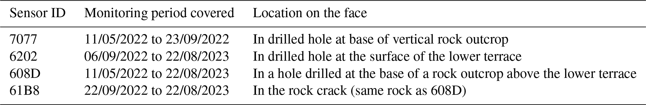
Four miniature temperature sensors (iButtons, Mouser^®) have been installed in holes drilled 5 cm into the rock surface, at the snow-rock interface, on the terraces where the fluorescent dyes were injected. The holes containing the coin-sized sensors were filled with gray polymer clay to insulate the metal sensors from direct solar radiation. The sensors monitored ground surface temperature (GST) at hourly time steps and over different periods (Table 1), but only one (#61B8) monitored the temperatures during both seasons.

Table 1 Miniature temperature sensors “iButtons” at the snow-rock interface.

Snow melting was identified as “zero-curtain” periods in GST (Fig. 5). These periods are characterized by stagnant GST at ∼0 °C (Hanson and Hoelzle, 2004; Staub and Delaloye, 2017). The complete melting of the snow is marked by the transition from dampened GST daily oscillations to positive and significant daily oscillations once the insulating snow layer has melted and solar radiation reaches the rock surface. As GST is measured at point-scale, it lacks spatial representativeness of the snow melting surface area. Thus, to complete this data, pictures were frequently taken during fieldwork in 2022 to document snow patch evolution. In 2023, an automatic camera was installed (Fig. 5) on a terrace of the North Pillar (See location on Fig. 1). From 1 March 2023 to 22 August 2023, it took 4 pictures a day of the north face of the Central Pillar, to monitor the snow patch evolution right above the water collection system. Pictures after 22 August 2023 are not usable because the protective glass was broken, and the pictures became blurred.

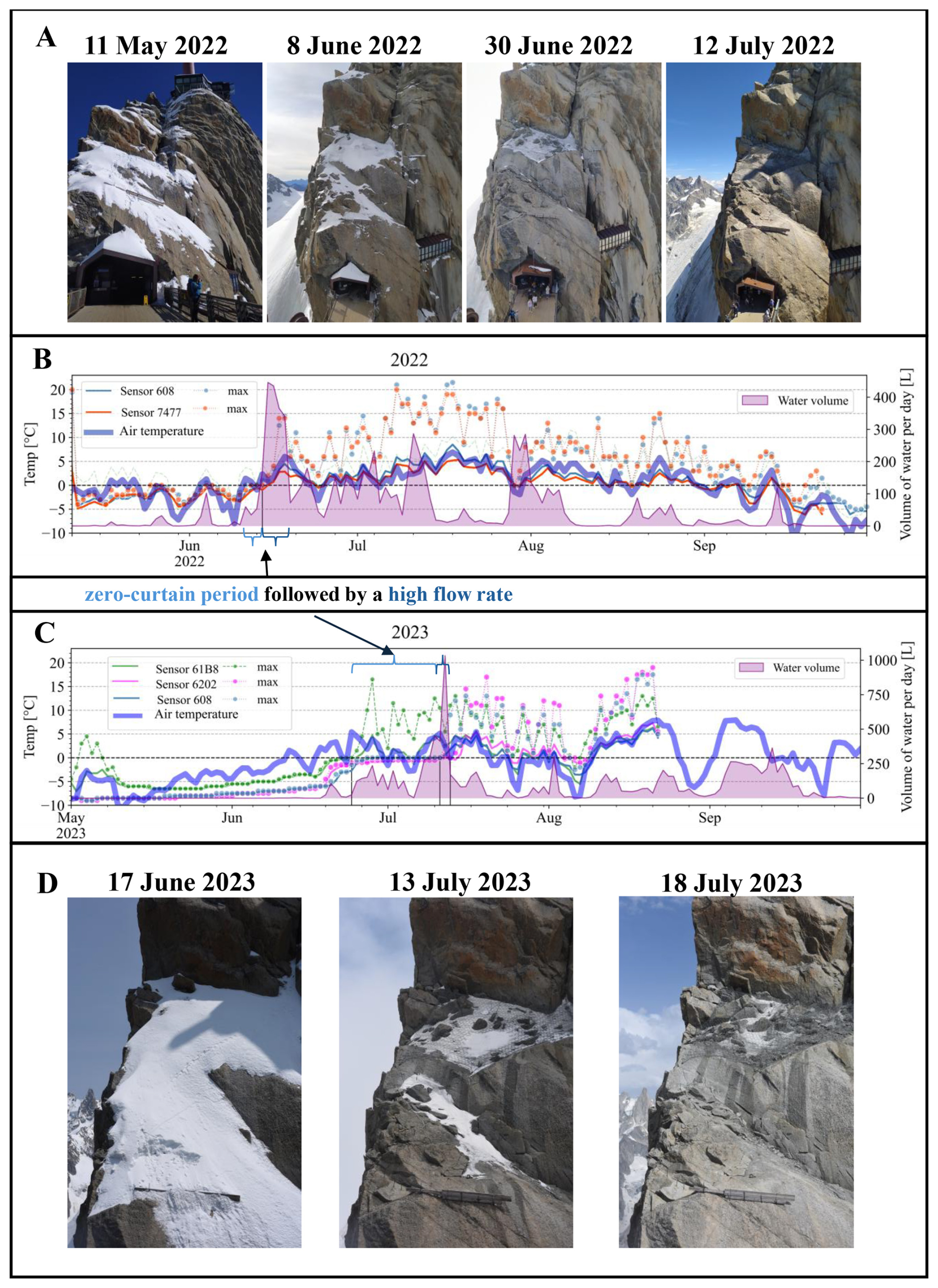
Figure 5 (A) Photos showing the evolution of the snow cover on the NE face during the snow melt season in 2022. (B, C) AT, GST measured on the NE face, above the tunnel entrance, directly above the monitoring system, and flow rate measured at the output from rock fractures in the tunnel wall (Box 1 + Box 2) in 2022 and 2023, respectively. Solid lines represent the daily average. Note the zero-curtain period, which marks the melting of the snowpack and the exposure of the rock surface to atmospheric heating. (D) Photos showing the evolution of the snow cover on the NE face during the snow melt season in 2023.

3.3 Water flows and temperature monitoring in the tunnel

We installed a real-time monitoring system in May 2022 in the west tunnel of the Central Pillar, to characterize the water flowing from fractures that cross the tunnel walls. We took advantage of an existing water diversion ceiling set up by the operating company (Fig. 4), made of a convex metallic plate that collects water drips and flows, and diverts them to two pipes, one on each side of the tunnel (east and west) to drain water outside. Preliminary observations revealed that water was mostly dripping from two adjacent fracture systems with a generally subvertical dip (70°, −90°) oriented toward north-west.

The instrumentation included two rain gauges that were installed on each pipe to measure water flow rate (L h⁻¹), in protective boxes (Box 1 on the west side and Box 2 on the east side). Water temperature (°C) and electrical conductivity (S cm⁻¹) were also monitored with sensors placed on the metallic roof, below the identified water drips. The sensors were submerged in a specially designed, 3D printed, siphon-shaped pipe (Fig. 4B) to maintain a high water exchange rate and a minimal water level for detection. As a conductivity benchmark, we measured a value of 9.2 µS cm⁻¹ from a melted snow sample collected on the 26 July 2023, which corresponds with known values for snowmelt samples (Brennan et al., 2020; Thompson et al., 2016). In addition, water fluorescence (arbitrary units) was monitored in real-time with a probe inserted in Box 1 to detect the specific emission spectrum of the dye tracer used: AAG and SRB in 2022 and AAG and FLC in 2023 (see Sect. 3.1 for dye spraying strategy). The fluorescence sensor installed in 2022 (GGUN FL-24) malfunctioned during the 2022 winter and was replaced by a new probe (STREAM model, TRAQUA^®) on the 31 May 2023 and was removed on 22 August several weeks after the last dye signal was detected.

Average values from the installed sensors were recorded every 10 min with a PC400 Campbell Scientific data logger. In addition, data from miniature temperature sensors (iButtons, Mouser^®) that were previously installed were used to monitor the tunnel wall (bedrock) temperature.

The site was visited weekly, excluding a short period from 25 July 2023 to 10 August 2023 because of a storm that prevented access, to retrieve data, take water samples and manual measurements on electrical conductivity, and to clean the rain gauge, since sediments sometimes accumulated (Fig. 4).

3.4 Water sampling in the tunnels and laboratory analysis

Water samples were collected weekly from Box 1 during the melting seasons of both 2022 and 2023. Other locations in the tunnel (labeled Box 2 and TNL) were sampled six times in 2022 and weekly in 2023. Samples were taken in 125 mL brown glass bottles. During the 2023 season, the electrical conductivity of each sample was measured directly after collection. The bottles were stored in a fridge to minimize biological activity and protect them from light.

Further high-resolution fluorescence analysis of the water samples was carried out in a laboratory, using a fluorescence spectrophotometer (Varian Cary Eclipse) to validate the real-time fluorimeter data. The samples were exposed to light whose wavelength spectrum matched the excitation spectrum of the dye tracers used in the experiment (AAG ex: 305 nm $/$ em: 447 nm, SRB ex: 555 nm $/$ em: 577 nm, FLC ex: 490 nm $/$ em: 510 nm). The emission vs. excitation wavelength plots were used to find peaks in emission distribution that corresponded to the presence of the dye tracers.

In addition to fluorescence analysis, we performed stable isotope analysis on 11 water samples to determine δ¹⁸O and δD values. Stable isotopes are widely used in hydrological studies to trace the origin and history of water, as their ratios are sensitive to fractionation during phase changes in the hydrological cycle. Such analyses can reveal important information about water sources (e.g. snowmelt vs. rainfall), transport pathways, and storage times. By comparing the measured isotopic signatures to the Global Meteoric Water Line (GMWL), we can assess whether the water follows typical meteoric patterns or has undergone secondary processes such as evaporation, mixing, or prolonged subsurface residence. Deviations from the GMWL can also indicate elevation effects or seasonal variations in precipitation, making isotope data a valuable complement to physical and chemical tracers in characterizing alpine hydrological systems.

3.5 Data analysis

We processed and analyzed the continuous time series data by developing codes in Python3 and MATLAB. All time series were filtered for erroneous values and linearly interpolated to evenly spaced time steps for consistency.

3.5.1 Recession curves analysis

Recession curves have been studied since the late 19th century (Brutsaert and Nieber, 1977; Tallaksen, 1995) and are commonly used in hydrology to interpret the flow behavior and characteristics of aquifers. A key advantage of this approach is that it allows the derivation of empirical, quantitative parameters that reflect the subsurface drainage. Following work by Boussinesq (1877), Maillet (1905) suggested an exponential analytical solution to describe aquifer drainage behavior:

$$\begin{array}{}\text{(1)}& Q\left(t\right)=Q_{\mathrm{0}}{e}^{-\mathit{\alpha }t},\end{array}$$

where Q is flow rate, t is time, Q₀ is peak flow rate, and α is the recession coefficient. To account for flood recession in a channelized flow, we opted for the general form suggested by Brutsaert and Nieber (1977) that is commonly used for river flood recessions (Brutsaert and Nieber, 1977; Krakauer and Temimi, 2011):

$$\begin{array}{}\text{(2)}& {\displaystyle \frac{\mathrm{d}Q}{\mathrm{d}t}}=-a{Q}^b,\end{array}$$

which can be integrated and solved for Q(t) as:

$$\begin{array}{}\text{(3)}& Q\left(t\right)=(Q_{\mathrm{0}}^{\mathrm{1}-b}-a(\mathrm{1}-b)t{)}^{\frac{\mathrm{1}}{\mathrm{1}-b}},\end{array}$$

where a and b are constant coefficients. Note that the integration of Eq. (2) in the case of b= 1 corresponds to the form of exponential decay as expressed by Eq. (1). Scandroglio et al. (2025) recently applied Maillet's law (Eq. 1) to analyze flow in fractures within a permafrost-affected rock wall in the Northern Calcareous Alps, at the German-Austrian border. Their study focused on a 55 m deep tunnel in karst limestones, where flow paths extend at least 55 m and possibly farther due to tortuosity. In contrast, in our study, flow is confined to widely open, sub-vertical granite fractures with path lengths ranging from 12 m (lower terrace) to 20 m (upper terrace). Additionally, while we define a flow event as the period between a well-defined rise and the following recession of the hydrograph, Scandroglio et al. (2025) defined an event as a flow period beginning with a sudden increase in discharge, independent of the starting value, and ending when the flow returns below a set threshold, potentially including several peaks. They applied a single best-fit curve to their entire dataset, which comprised 23 such high-flow events over eight years. Their approach is well suited to rain-controlled conditions. In contrast, our field site at 3840 m a.s.l. is dominated by snowmelt and thus strongly influenced by the diurnal solar cycle. We therefore identified 93 well-defined single-peak events for recession-curve analysis over two consecutive seasons. To capture temporal variations in flow rate, we developed an automated algorithm that fits a separate recession curve to each event, enabling to track changes in flow behavior over time (Figs. S2, S4). For each event, the algorithm identifies the recession limb as the interval between the last local maximum and the subsequent return to baseflow. It then isolates the concave segment of this limb (curvature > 0), which corresponds to the exponential decay, and fits the appropriate form of Eqs. (1) or (2). To ensure that only well-defined exponential recessions are included, events with regression fits yielding R²< 0.8 are discarded. This threshold retains 64 % of all detected events (93 out of 144) while excluding cases where noisy or multi-peak recession behavior prevents reliable fitting.

3.5.2 Moving window cross-correlation

To quantify the temporal relationship between flow rate, AT, and GST, we performed a moving-window cross-correlation analysis based on the Pearson correlation coefficient (PCC) (Pearson, 1920). For two time series x(t) and y(t), the PCC value (r) at lag τ was defined as:

$$\begin{array}{}\text{(4)}& r\left(\mathit{\tau }\right)=\mathrm{corr}\left(x\left(t\right),y\left(t+\mathit{\tau }\right)\right)\end{array}$$

where positive lag values (τ> 0) indicate that variations in x follow those in y after a delay τ. Lag times were evaluated in the range −12 to +12 h with a step of 1 h, consistent with the expected diurnal forcing of temperature and flow. The use of cross-correlation analysis to assess time-lagged relationships in hydrological time series is well established (e.g., Delbart et al., 2014).

This analysis was applied within successive 24 h windows starting at 00:00 CEST (UTC+2), without overlapping, corresponding to the dominant daily cycles observed in flow and temperature. A 24 h window length has been chosen as a compromise between diurnal variability resolution and statistical robustness of the correlation estimates.

Prior to analysis, all the time series (time step =10 min) were filtered using a 1 h moving average to reduce high-frequency instrumental noise. This smoothing window is substantially shorter than the dominant diurnal signal and does not affect the identification of lag times at hourly to multi-hour scales, but improves the stability of the correlation estimates.

To ensure that meaningful diurnal responses were analyzed, only days with a maximum flow rate exceeding 6 L h⁻¹ were included. This threshold excludes low-flow days dominated by noise or weak signals and focuses the analysis on periods with well-defined hydrographs.

The analysis was conducted over the entire flow season (mid-May to August 2022; June to September 2023).

4 Results

4.1 Water flow rate

Water flow is highly seasonal. In both years, water mostly flowed between May and October, with periods of sporadic and continuous flow that can last several weeks. The occurrence of water flows correlates with the occurrence of positive AT (Fig. 5).

In 2022, sustained periods of water flow were mainly observed from late May to mid-September, and in 2023, from mid-June to late September. The timing and magnitude of the flow differed between Box 1 and Box 2 (Fig. 6). In both years, water flow in Box 1 began several weeks earlier than in Box 2. In general, the amount of water in Box 2 increased throughout the summer season.

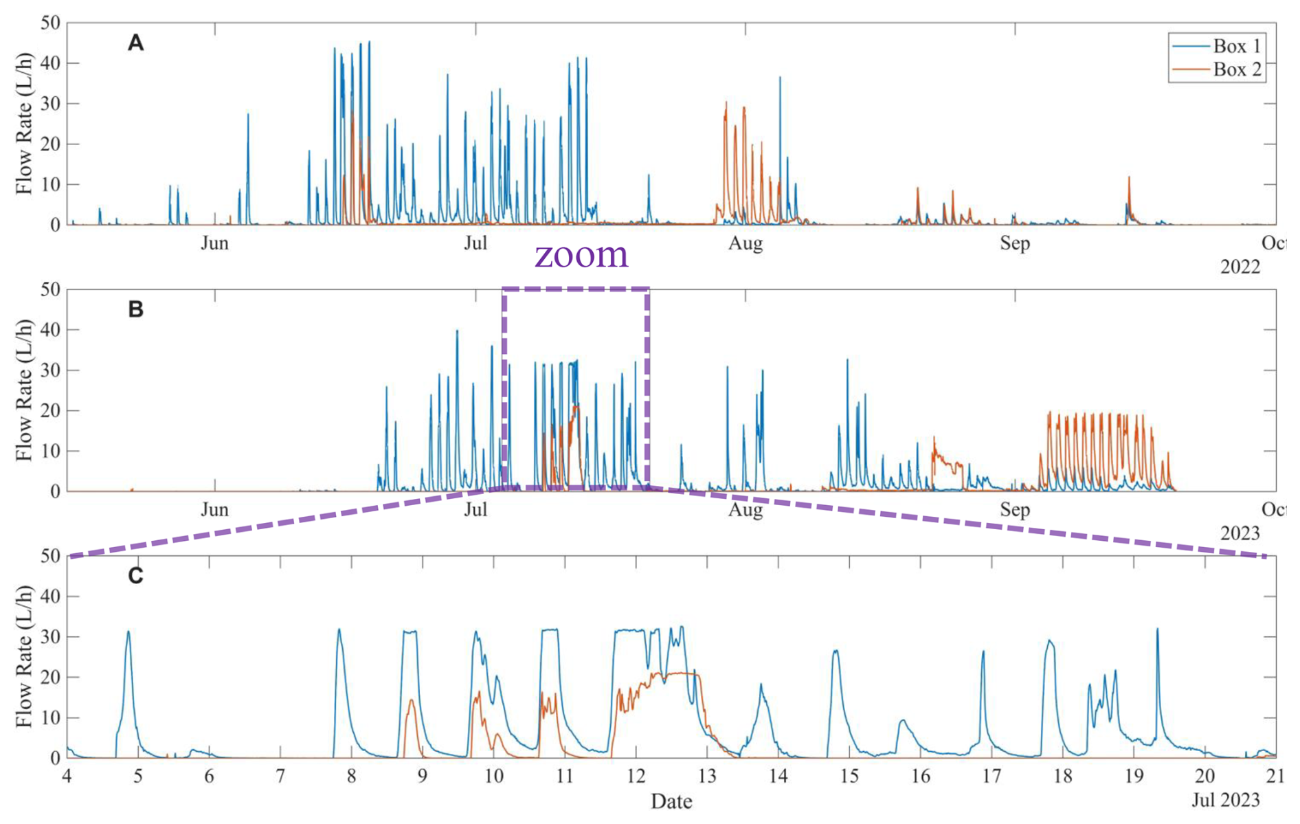
Figure 6 (A, B) Time series of flow rate in Box 1 (blue) and Box 2 (orange) during the 2022 and 2023 melt seasons, respectively. (C) Zoom window on the 4–21 July 2023 period.

In 2022, the total volume of water flowing through the monitoring system (Boxes 1 and 2) was 8001 L. About 70 % of this volume (5621 L) was collected in Box 1, while the remaining 30 % (2380 L) reached Box 2. 75 % of the total volume in Box 1 occurred between 11 June and 14 July (4216 L). Of the total flow volume in Box 2, 74 % flowed in two relatively short periods: 14–19 June (496 L) and 28 July–8 August (1257 L).

In 2023, the total volume of water flow was 11605 L, 45 % more than in 2022. Of this, 61 % (7079 L) flowed through Box 1, and 39 % (4526 L) in Box 2. 75 % of the total volume in Box 1 occurred between 19 June and 10 August (5309 L). In Box 2, almost the entire volume (95 %) flowed in three relatively short periods (3 to 18 d): 8–13 July (831 L), 22–25 August (611 L), and 1–18 September (2851 L).

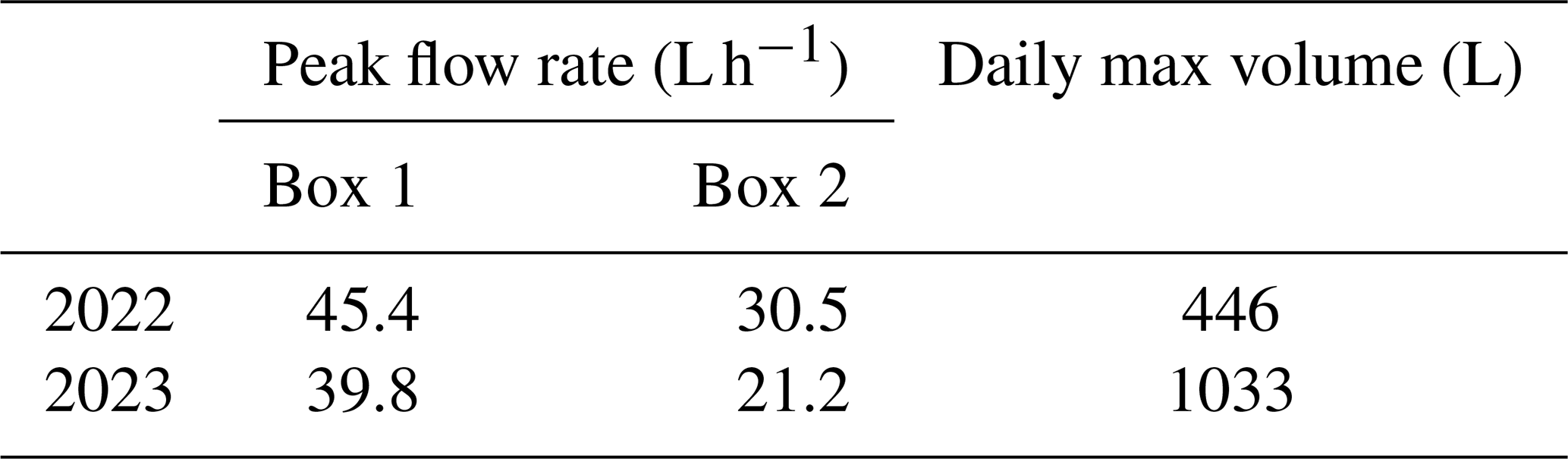
The observed flow rate presents daily cycles (Fig. 6) with peak flow rates, reaching an order of 10¹ L h⁻¹, generally occurring between 17:00 to 20:00 (Table 2, Fig. S1), and minimum flow rates two orders of magnitude lower (order of 10⁻¹ L h⁻¹) during the morning time.

Table 2 Time of day of the daily peak in flow rate, AT, and GST. The listed time ranges represent the 25 %–75 % quantile of daily peak timing.

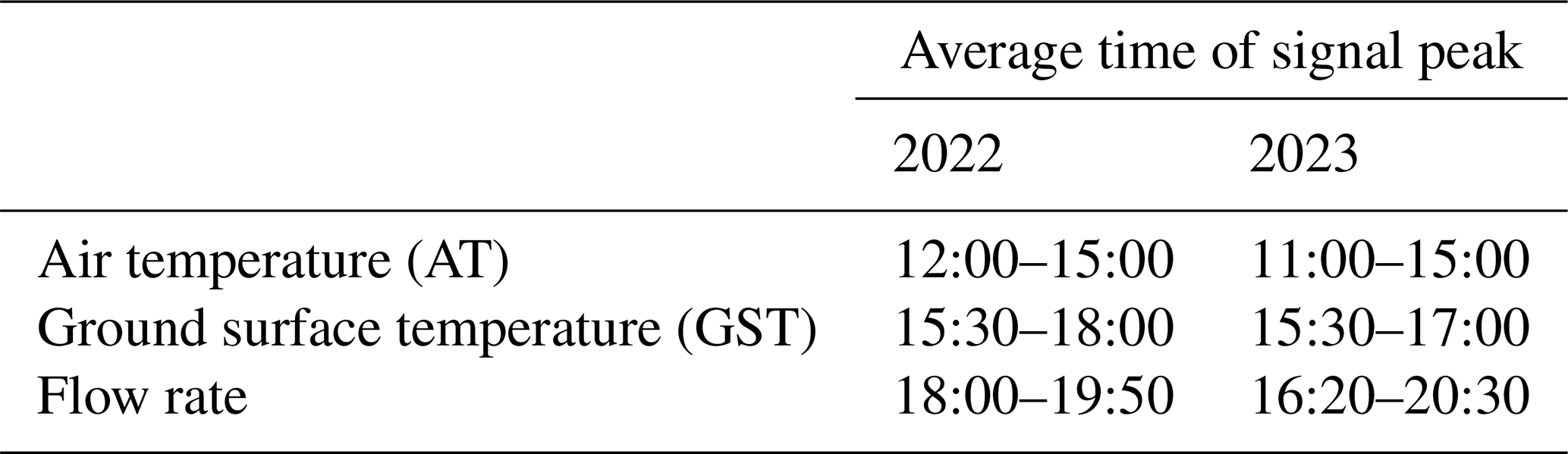
Results of a moving window cross-correlation show that daily flow rate oscillations are correlated with AT with a lag time of 3–9 h, and with GST with a lag time of 0–6 h. This lag time was found to be steady in both years of the experiment (Table 2, Fig. 8).

In 2022, the first flow in Box 1 was recorded on 15 May (1.1 L h⁻¹) and gradually increased, reaching continuous daily flows with peak values larger than 40 L h⁻¹ from 11 June to 14 July, after which flows were linked to rainfall. Box 2 showed its first significant flow (>10 L h⁻¹) on 15 June, with continuous daily oscillations lagging about 5 d behind Box 1. Maximum flow rates were 45 L h⁻¹ in Box 1 and 30 L h⁻¹ in Box 2, with a combined peak of 67 L h⁻¹ on 16 June.

In 2023, Box 1 exhibited continuous daily oscillations from 19 June, peaking at 40 L h⁻¹ on 28 June, interrupted by short cold spells, and resuming under positive AT and precipitation events (Fig. 6). Box 2 began daily flows between 8–13 July (up to 20 L h⁻¹) with a prolonged steady flow (5–12 L h⁻¹) from 22–25 August despite minimal precipitation. Maximum individual flows were 39.83 L h⁻¹ in Box 1 and 21.20 L h⁻¹ in Box 2, with combined peak flow of 54 L h⁻¹ on 12 July. Daily maximum volumes reached 446 L in 2022 and 1033 L in 2023 (Fig. 6).

Table 3 Flow rates peaks.

The exponential recession curves (Eq. 1) fit well with the observed daily events, with an average R² value of 0.93. Curves with R² values below 0.8 were omitted from the analysis, resulting in 93 events (Fig. 9). The a coefficient shows a clear decreasing trend in time from values of 7–10 to 5–8.5 in both 2022 and 2023 seasons (Fig. 9), while the b coefficient increases from values of b≈ 1 at the beginning of the melting season to values of b≈ 1.15 at the end of the season (Eqs. 2 and 3).

4.2 Snowpack evolution and water flow characteristics

Snowpack evolution is assessed through GST measurements at the snow-rock interface and using time-lapse pictures in 2023. Dampened daily oscillations in GST indicate the presence of a snowpack with a significant insulating effect. The melting period is generally visible as a zero-curtain period (i.e., persisting 0 °C conditions at the rock-snow interface) (Hanson and Hoelzle, 2004) that lasts from several days to several weeks.

Figure 5 displays the measured GST data at the rock-snow interface. In 2022, the dampened daily oscillations are revealed by the similar values of mean and maximum GST, and the zero-curtain period is nearly nonexistent. This could be related to the early heat wave in 2022 that accelerated snow melting. Nonetheless, the first water flow events in May and early June 2022 occurred when GST rose close to 0 °C, demonstrating a link with snow melting. The first significant water flow event in 2022, which is also the greatest one with values reaching over 400 L d⁻¹, coincides with the transition to positive GST around mid-June. Summer precipitation episodes are suggested when water flow events follow periods with limited water flow and positive GST and AT, such as in late July 2022. In 2023, the effect of snow cover on GST patterns is more evident, with an initial period of non-existent daily oscillations followed by a zero-curtain period until mid-July. The first flow events occurred during the onset of the snow melting period, with the highest peak of water flow reaching >1000 L d⁻¹ at the end of the zero-curtain period.

4.3 Fluorescence

4.3.1 Real-time fluorescence monitoring

In 2022, the real-time fluorescence sensor shows a strong signal of AAG that followed the very first flow events in mid-May 2022 (Fig. 7) and the sporadic flow events that followed it until 11 June 2022. The high AAG signal continued with the onset of continuous water flows around mid-June 2022, until the rapid decrease at the end of June. The disappearance of the fluorescent signal, despite the sustained water flow likely corresponds to the complete melting of the lower terrace snowpack that contained the AAG tracer, as seen in the photos from the time lapse camera (Fig. 5). A weak signal of AAG was detected until mid-July 2022 when both the fluorescence and flow rates diminished. This period of weak AAG signal in the water could indicate dilution with water from precipitation that occurred after the dye was inserted or another not-dyed source (either late snow or rain). No signal of the SRB tracer inserted in the upper ledge was found. This could be due to excess dilution of the tracer solution with the snowmelt water to concentrations that were below the sensor sensitivity. A second hypothesis is that snowmelt from the upper terrace did not reach the fracture. In 2023, AAG signal was also detected in the first water flows on 19 June. From the 24 June 2023 onwards, the signal of the FLC dye was detected alongside AAG, which likely confirms that the concentration in SRB was probably too low in 2022. The FLC signal is shorter than the AAG signal, with a single high peak in the last week of June followed by a rapid decrease to low values. This could be explained by the different pathways from the upper terrace snowpack through the fracture network, together with the effect of low dispersivity of FLC. The high peaks of AAG persisted continuously until 8 July. Afterward, both tracers remained in low concentrations until the end of July, suggesting that much of the winter and spring snow had melted by 27 July. That could mean that the time needed for the entire winter snowpack to infiltrate is slightly more than a month. After that, the water flowing from mid- to late July was either direct precipitation (rain and snow) or possibly meltwater from ice that predated the tracer insertion.

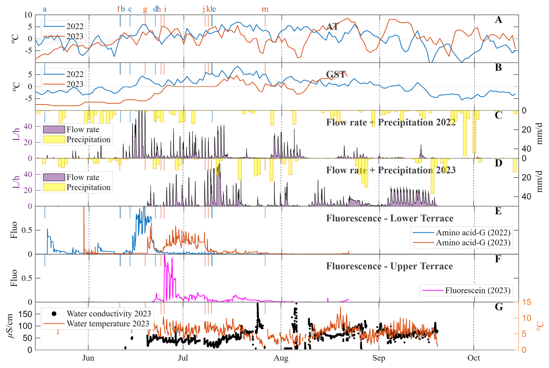
Figure 7 Annual time series. (A) Air temperature (AT) measured by Météo-France in Aiguille du Midi. (B) Ground surface temperatures (GST) measured using miniature temperature sensors (iButtons) at the rock surface on rock slope. (C–D) Flow rate measured in both box 1 + box 2 (purple) and daily precipitation measured in Chamonix meteorolocical station (Météo-France) (yellow bars). (E) Normalized fluorescence signal of amino acid-G dye tracer (2022 and 2023). (F) Normalized fluorescence signal of Sulphorodamine-B (inserted in 2022) and Fluorescein (inserted in 2023) dye tracers. The Sulphorodamine-B dye was never detected. (G) Water conductivity and temperature at the outlet of water from the fracture in the tunnel. Measurements in time steps without water flow were omitted from the plot. Labeled annotation at the top of panel (A) mark the following main events in 2022 (blue): a) first flow event in box 1, b) AT surpasses 0 °C, c) GST surpasses 0 °C + beginning of daily oscillations + first flow in box 2, d) amino acid G signal diminishes, e) last amino acid G signal, and 2023 (orange): f) AT surpasses 0 °C, g) first water flow event in box 1, h) beginning of daily oscillations, i) beginning of zero curtain, j) first flow in box 2, k) amino acid G signal diminishes, l) end of zero curtain, m) last amino acid G signal.

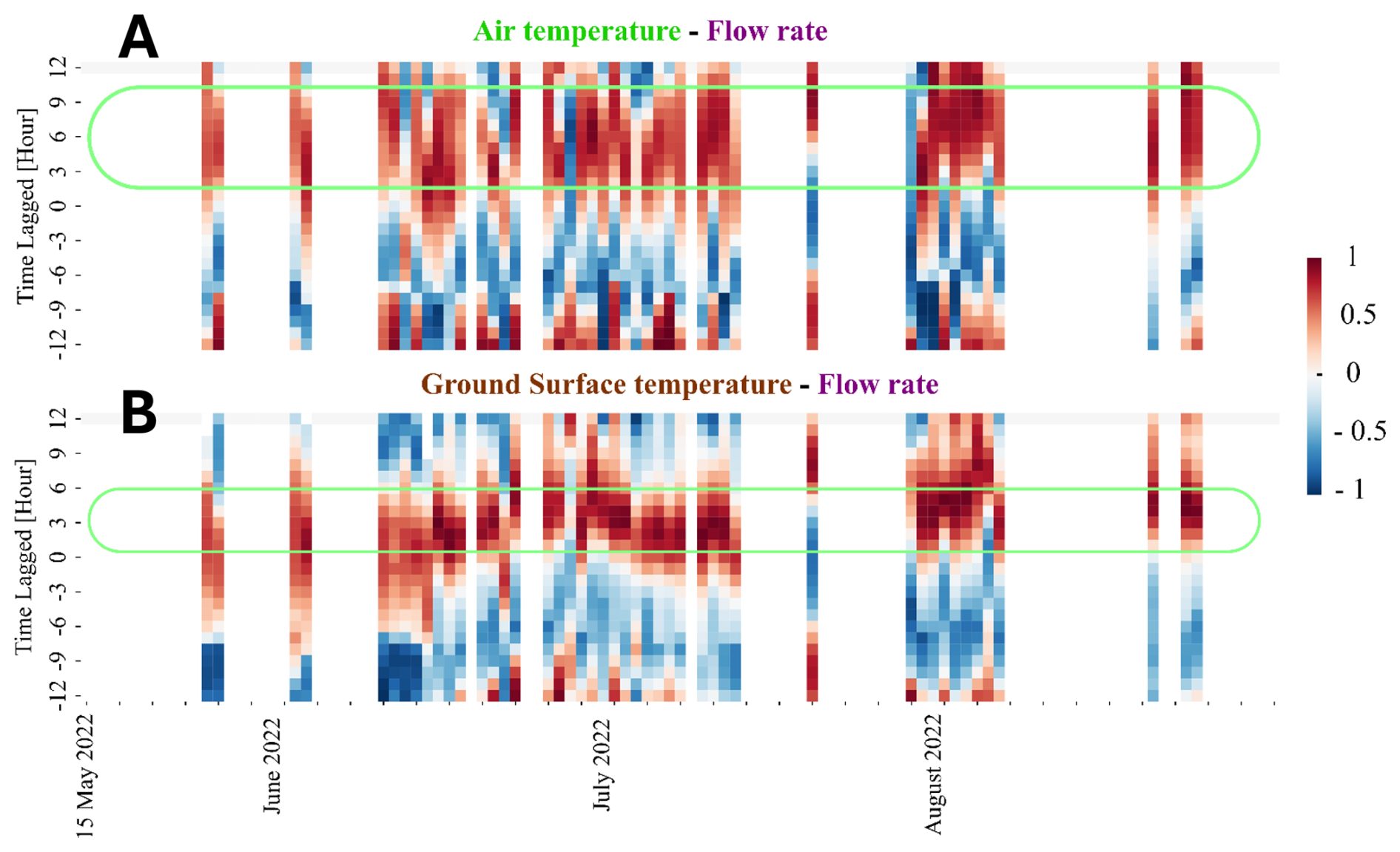
Figure 8 Results of moving-window cross-correlation analysis between the water flow rate and the (A) air temperature and (B) the ground surface temperature, during 2022 season. The horizontal axis represents the time (one strip per day), and the vertical axis represents the lag time, in hours. The color bar represents the value of the Pearson correlation coefficient (PCC) (1: high correlation, 0: no correlation, −1: reverse correlation). The green frame marks the range of lag times that show high PCC. Results of the cross-correlation analysis of 2023 season show similar results and can be found in the supplementary materials, in Fig. S3.

4.3.2 Fluorescence laboratory results

Additional analyses of water samples collected between May and mid-July 2023 from Boxes 1 and 2 and various fractures dripping into the tunnels of AdM were carried out using a high sensitivity spectrophotometer in the EDYTEM laboratory. The results are similar and confirm those found using the TRAQUA real-time sensor in Box 1. The signals for FLC and AAG show peaks at the same periods, i.e. at the end of the month of June and the beginning of July. The FLC signal is very short-lived, unlike AAG, which continues to appear for a longer period. Samples from other locations in the tunnel show no signal of any of the fluorescent dyes.

4.4 Stable isotopes

Analysis of oxygen and hydrogen isotopes in the water samples shows that δ¹⁸O and δD values range between −3.2 ‰ to −10 ‰ and −15 ‰ to −73 ‰ respectively (Fig. 10). Excluding two samples, the δ¹⁸O $/\mathit{\delta }$D ratio in all the water samples fall close to the global meteoric water line (GMWL) or align on a straight line parallel to the GMWL, likely because of a seasonal evolution of the local meteoric line from the GMWL (i.e. three samples taken on 22 September-labeled _22SEP). Two samples taken on 28 July 2022 from Box 2 deviate significantly below the GMWL (BOX2_28JUL – directly from the fracture, BCKT2_28JUL – from a 5 L bucket that collected the water from the fracture) (Fig. 10). This suggests that the water emerging from the fracture above Box 2 on that day was not of recent meteoric origin.

4.5 Water electrical conductivity

Electrical conductivity values are provided as maximum values per day of flow, after correction to a standard temperature of 25 °C. The electrical conductivity measurements from the 2022 season were unreliable due to the erroneous installation of the sensor. Therefore, only the 2023 results are presented and analyzed (Fig. 7). Overall, the conductivity values were far above the benchmark value measured in melted snow samples (9.2 µS cm⁻¹). On the continuous measurement (real-time monitoring system), the electrical conductivity of the water flowing into Box 1 remained relatively constant from mid-June to mid-July, with daily oscillations between 10–55 µS cm⁻¹ and a general decreasing trend. The daily oscillations correlate with flow rate in a reverse relation – when flow rate is high the conductivity decreases (Fig. 7). These values of conductivity correspond to the period of continuous cyclic flow rate in Box 1 that ended with the complete thaw of the winter snowpack. Interestingly, significantly higher conductivity values were measured at other locations in the tunnels. Conductivity measurements with values of 485 µS cm⁻¹ were taken in a tunnel wall under the west face of the central peak, from mid-July onwards, and 430 µS cm⁻¹ (measured in 2022) at another location in a tunnel under the north-east face of the central peak, near the exit of the cable car going to Pointe Helbronner (Italy).

4.6 Water temperature

During flow events, the water temperature measured in two locations at outputs from the fractures ranged between 0 and 13 °C with an average of 6.1 °C (Fig. 11). Measurements taken during periods without flow or subzero temperatures were removed from the analysis. Average GST and AT during the thawing season (15 May to 15 September) are close to 0 °C. Values measured at the rock surface in the tunnel walls, near the fractures, during flow events show an intermediate mean value of 3.0 °C.

5 Discussion

5.1 Water flows and weather conditions

Our results show rare evidence of highly effective surface-subsurface connectivity in steep permafrost-affected slopes, and strong weather signals in both seasonal and diurnal scales. There is a clear link between the timing of AT and GST becoming positive in the early summer months and the onset of water flow. The first flow events in the season, which appeared in early May (2022) and June (2023), display a clear signal of the dye tracer and are directly linked to snow melting occurring under positive AT in the relatively shaded north-exposed rock face.

In both years, the onset of water flow in the fractures occurred when the daytime AT reached values above 0 °C. This change in temperature to positive values directly induced the melting of the snow that was deposited during winter, and its infiltration into the fractures. The melting of the snowpack is demonstrated by the simultaneous detection of the fluorescent dye tracers injected into the snowpack and the zero-curtain effect observed in the GST (Figs. 5, 7). The melting accelerated when the rock surface was exposed to heat flux from the atmosphere and GST turned positive. From this point onwards, water flow behavior became more uniform, with regular daily oscillations, and reached the highest flow rates. Subsequently, after the exposure of the rock surface, some of the water in the fracture was directly from precipitation, which likely melted rapidly on the rock surface as the temperature increased, often above 0 °C. Each year, water flow in the fractures ceased when the temperature became negative again in autumn, with icicles appearing in the fractures.

Based on the 2-year monitoring, we conclude that water flow processes in high mountain rock faces are therefore seasonal, directly linked to the change in air and surface temperatures to above 0 °C during the summer period and below 0 °C during fall. The continuous detection of the dye, together with an analysis of time-lapse photos of the rock face and the shift of GST to positive values, show that snowmelt is the main source of water in the fractures during the early and main stages of flow, and contributes most of the water. This is consistent with similar observations reported by Scandroglio et al. (2025).

GST and AT also control flow rate oscillations on a daily time scale and are cross-correlated with a lag time of 3–9 and 0–6 h, respectively (Table 2, Figs. 8, S3). These lag times provide an estimation of the time taken for water to travel through the fracture system, and allow a rough approximation of flow velocity on the order of ∼10 m h⁻¹.

The observed acceleration in flow rate coincides with the heating of the rock surface to above 0 °C and points to a top-down thawing of the active layer (i.e. the near-surface layer that freezes and thaws through summer).

Nevertheless, the time lag between surface signal and water flow as well as the thawing of the active layer must be cautiously considered as it is possibly influenced by the open-system of the tunnel causing an open flow path and a thermal shortcut allowing for bottom-up heat transfer. In addition, the touristic infrastructure and human presence can contribute to internal heat sources, including heating systems, the elevator motor, and body heat from visitors (Fig. 11).

5.1.1 Heat waves effect

The contrast in summer conditions between 2022 and 2023 further illustrates the strong influence of weather conditions on the timing and characteristics of the water flow period (Sect. 2.2). This is well demonstrated by the effect of the early heat wave in spring 2022 that resulted in an early onset of water flows and the late heat wave in autumn 2023 that extended the water flow period much later in the season. The 2023 season was significantly wetter in terms of precipitation, and subsequently, more water flowed in the monitored fractures. However, comparing the monthly distribution of flow during the thawing season reveals that it was greatly influenced by the heat waves. Between May to mid-July, flow volume in 2022 was much higher than in the same period in 2023, as a result of the early and rapid thawing. Only in late August did the total volume of water flow surpass that of 2022. This raises an interesting point for future research on the influence of early vs. late water infiltration in permafrost rocks and the impact on hillslope processes. Assuming that water that infiltrates later in the season is warmer than the rock mass, and the infiltration paths contain less ice, it can potentially accelerate permafrost degradation and thickening of the active layer.

Compared to the less extreme spring temperatures in 2023, the rapid thaw in 2022 is evident in the GST data and in the absence of a zero-curtain period, which is clearly observed in 2023 (Figs. 5, 7). We suggest that during the early heatwave in 2022, there was less snow, the thawing was very rapid, and the latent heat was absorbed rapidly. This can be seen in Fig. 5, which shows less snow cover in min-June 2022 in comparison with mid-June 2023, and a large volume of water immediately after GST turns positive.

5.2 Water flow path conditions

Our results also indicate that an effective pathway exists within the fracture network through which the water released by snowpack melt can infiltrate at the end of spring. The early detection of fluorescent dye in the first flow events suggests a relatively rapid transfer from the surface to the fractures. Furthermore, when flow ceases at the end of autumn and icicles form at the fracture outlet, the observed flow appears to be unsaturated. In such cases, the unsaturated flow is likely routed through preferential pathways within the fracture system, which in turn suggests that at least part of the network remains open and able to convey meltwater during the following spring. However, we cannot overrule the possibility that the man-made space of the tunnel contributed to the unsaturated conditions. In natural conditions, if undrained conditions occur, water could accumulate in the fractures, refreeze inside them, and seal them off. Artificial prevention of ice accumulation can inhibit fracture development through ice segregation and the related cryostatic pressure (Draebing et al., 2014; Draebing and Krautblatter, 2019; Hales and Roering, 2007; Hallet et al., 1991; Matsuoka and Murton, 2008; Matsuoka and Sakai, 1999). Completing these water flow observations with crack-meters to measure fracture rheology would provide an interesting perspective to clarify the role of the tunnel. However, this would require identifying the fractures that are directly connected to the tunnel.

Interestingly, our monitoring system shows different but consistent timing of water flows in Boxes 1 and 2, despite them being located only a few meters apart (Fig. 6). One reason for the delayed flow in Box 2 could be linked to the location of the draining area closer to the colder north face, while the draining area of Box 1 is closer to the west face, which receives more solar radiation. Another explanation could be suggested based on the observed accumulation of sediments in Box 2, which was not observed in Box 1. The origin of the sand-size sediments observed in Box 2 is very likely from the erosion of the granite rock. This suggests that the fracture system drained to Box 2 is filled with sediments that reduce the hydraulic conductivity. However, once flow begins in Box 2, it responds directly to precipitation and positive AT and reaches high flow rates, similar to those measured in Box 1 (e.g. in September 2023, Figs. 6, 7). This supports the first hypothesis of different exposures to solar radiation. The effect of the sediments filling on the hydraulic conductivity is thus reduced in late summer, perhaps due to the thawing of ice-filled pores within the sediments filling. Alternatively, the sand and ice in the sub-vertical fractures might act as a partial plug that accumulates water above the infill. When the hydraulic head is high and the ice filling is thawing, the plug can break, allowing the sand to be transported, and causing a change in the flow regime (as it was observed in Box 2).

Based on the delayed onset of flow into Box 2 and the different flow behavior when compared with Box 1, we suggest that the two boxes collect two different flow pathways which have some common parts. As Box 1 and Box 2 are located approximately 3 m apart, we suggest that the fracture network is complex under the north face. Some parts of the network contain sand-size sediments, which probably explain the late and lower flow of Box 2. Other parts of the network lack sand filling and have a different hydraulic behavior. The effect of the sediment infill on fracture hydrology should be investigated further.

5.3 Deciphering possible water sources

According to the fluorescence data and the water flow timing, much of the collected water originates directly from recent snowmelt. This is also supported by the stable isotopes analysis of water samples from Box 1 (Fig. 10) which display values that are consistent with those reported in high-elevation mountain regions, such as the Alps (Lauber and Goldscheider, 2014), the Pyrenees (Herms et al., 2019), and Northern China mountains (Sun et al., 2016). It is also very likely that rain in late summer infiltrated the rock fractures and contributed to the flow. However, some data also hints at other possible sources of water. First, even the lowest values of electric conductivity of the water are far above the expected snow melt conductivity and they steadily rise with decreasing flow rate. The surprisingly high electric conductivity found in some samples collected from fractures (>400 µS cm⁻¹) can point to long residence times in the rock. Considering the results from the fluorescent dyes and the hydrological behavior, the flow path is very short (in both distance and time), thus ruling out a long exchange time between the surface water and the rock. It is possible that recent meteoric water was mixed with older water that was trapped as ice in the permafrost-affected rocks. This is also supported by the observed change in the shape of the recession curves over time (Fig. 9). The recession curves at the beginning of the melting season (May–June) show values of b≈ 1 and fit well with the exponential form that is expressed in Eq. (1). The early-season recession curves are also characterized by high values of a. Over time, the value of b increases linearly to a form better described by Eq. (3), while the value of the a coefficient decreases. This change in recession form (Fig. S4), from aquifer-type (Eq. 1) to channel-type (Eq. 3) can be explained by the thawing of ice in wide sub-vertical fractures that are likely to react more individually (rather than as a network) and enable rapid flow in the fractured granite. The decrease of a is non-trivial since one could expect that the drainage would be more efficient and with shorter recession time (i.e. higher a values) as the thawing of ice in the rock fractures progresses. We thus suggest that the observed decrease in a is due to a gradual change in the water source. As less water drains from the surface (after the complete thawing of the winter snow) and more water drains from the subsurface ice trapped in the fractures, the hydraulic gradient is reduced, and the duration of the recession is extended. Another evidence of a possible fossilized source can be seen in samples collected from Box 2 on 28 July (BOX2_28JUL, BCKT2_28JUL) which show an isotopic signal that is distant from the meteoric water line (Fig. 10). One possible explanation is an extended residence time within the fracture system, allowing for interactions with the surrounding rock. Water samples collected during the peak of summer, on July 28 (BOX2_28JUL, BCKT2_28JUL) and August 9 (BOX1_9AUG, BCKT2_9AUG), from both collection systems (Box 1 and Box 2) exhibit relatively enriched δ¹⁸O and δD values compared to those taken in early summer and fall. This enrichment may indicate the partial melting of seasonal snow. In contrast, two other samples from different locations within the AdM tunnels (TNL_9AUG and BRCK_28JUL), collected on the same dates do not show this enrichment. The observed δ¹⁸O and δD enrichment during summer is consistent with findings from the Alps (Lauber and Goldscheider, 2014; Novel, 1995).

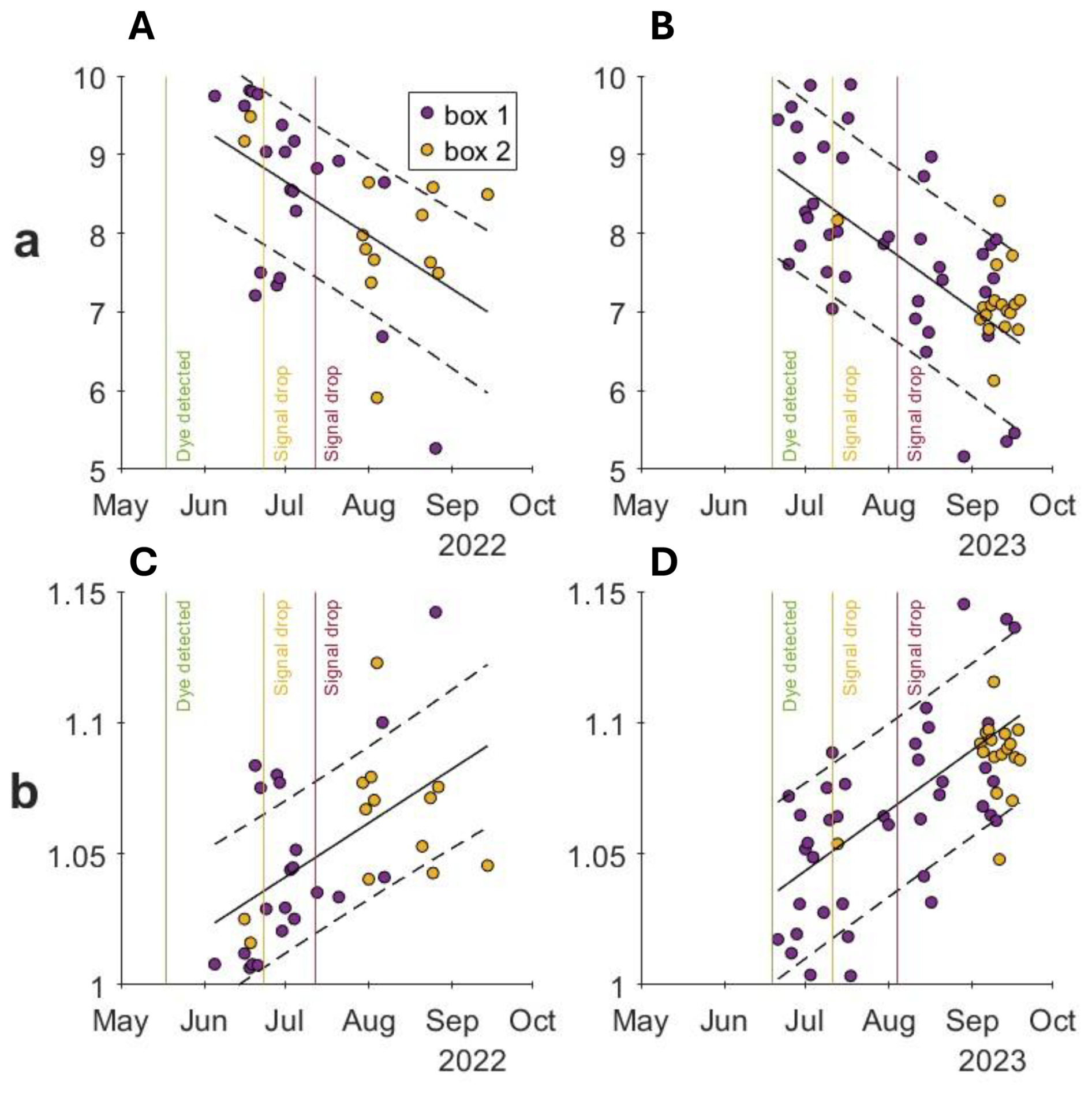
Figure 9 (A–B) values of the a coefficient of the recession curves of flow events in 2022 and 2023 in box 1 (purple circles) and box 2 (yellow circles). (C–D) values of the b coefficient of the recession curves of flow events in 2022 and 2023 in box 1 (purple circles) and box 2 (yellow circles. Values obtained from curves with R² values below 0.8 were omitted from the analysis. The black line is the linear regression of all the points (box 1 + box 2) with ±standard error (dashed black lines). The vertical lines indicate the timing of the detection of the fluorescent dye in the water that exits the fractures (green), the rapid drop of the signal intensity (orange), and the disappearance of the signal (red).

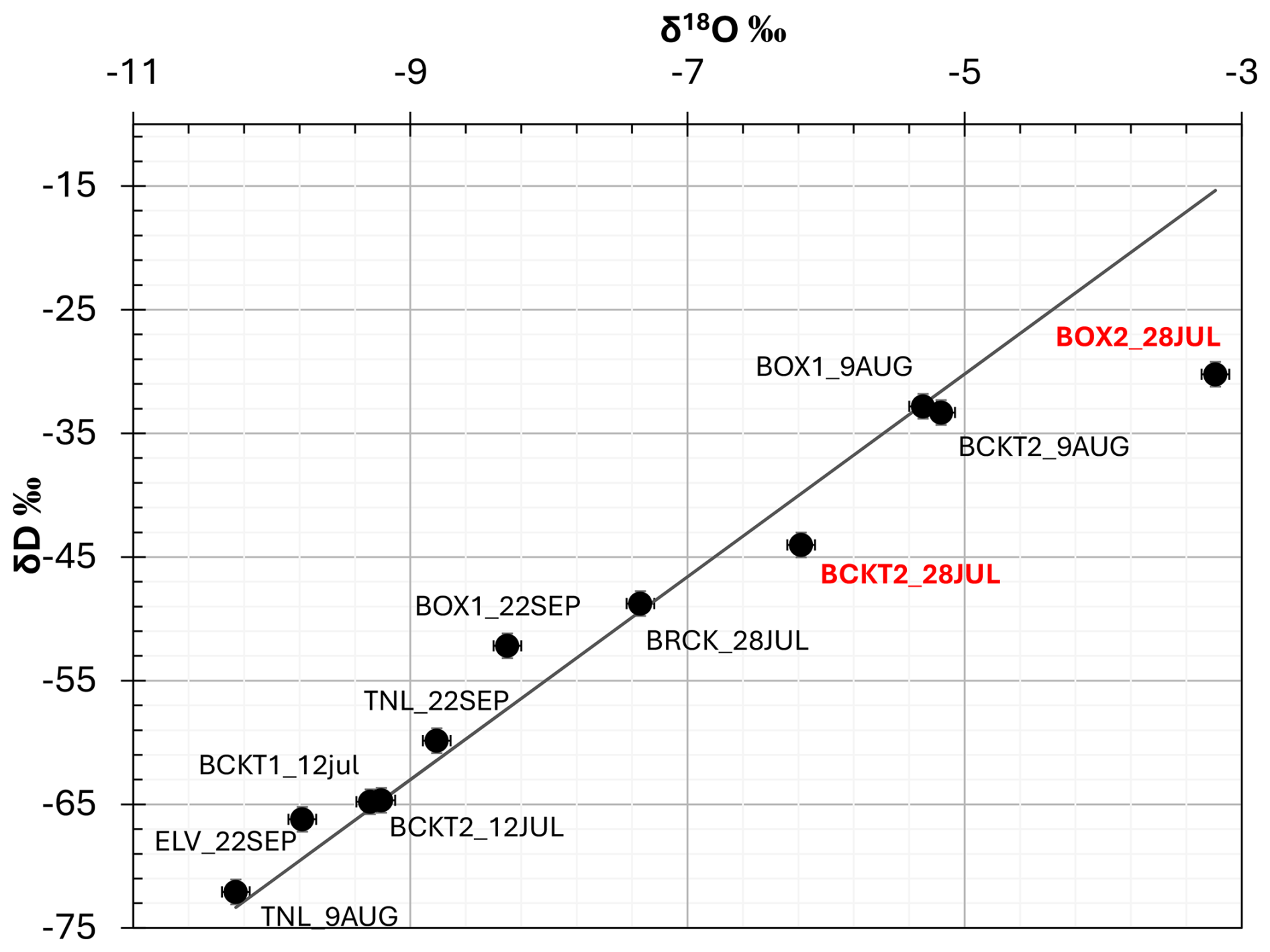
Figure 10 Stable isotopes δ¹⁸O and δD in water samples. Note the two outliers (labeled in red) from the global meteoric water line (GMWL, black line) in samples taken from Box 2 on 28 July 2022.

From a permafrost perspective, the thawing of large volumes of fossilized water in permafrost-affected rock could be related to a thickening of the active layer and degradation of high mountain permafrost – a regional phenomenon seen in recent decades in boreholes in the Alps and other mountain ranges (Magnin et al., 2024; Noetzli et al., 2024), but never observed directly in water samples from fractures.

The absence of a signal from SRB tracer in the water from the upper ledge could be due to excess dilution of the tracer solution with the snowmelt water, resulting in concentrations below the sensor sensitivity. In 2023, a different dye was used (FLC), with a significantly higher concentration (see Sect. 3.1), and was clearly detected, confirming that the absence of a SRB signal in 2022 was due to dilution.

5.4 Implications for alpine geomorphology, hydrogeology, and permafrost

The quantity, timing, and characteristics of water that infiltrates in the fractured, permafrost-affected rocks are important factors in many geomorphological, hydrological, and geomechanical processes. However, our understanding of the parameters controlling these factors is limited, as is the ability to measure them. For example, the timing and quantity of water availability from snowmelt are often estimated indirectly using numerical models of energy and water mass balance (Ben-Asher et al., 2023; Lehning et al., 1999; Leinauer et al., 2021) and snowpack physics (Lehning et al., 1999; Vionnet et al., 2012). However, the outputs of such models depend strongly on the meteorological forcing used to drive them, and on hydrogeological parameters that are usually poorly constrained. The results of this study provide direct observations that can help to reduce these uncertainties and improve our understanding of water availability for infiltration and its environmental controls.

The new information that we provide regarding water flow in permafrost rock fractures can also be used to improve coupled heat and water flow models, as it provides the parameters needed to calculate heat advection from the surface (flow rate and water temperature). The average water temperature measured during flow events is 6.1 °C (Fig. 11) (Magnin and Josnin, 2021).

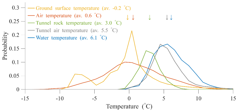
Figure 11 Probability distribution of temperatures monitored during flow events (blue), atmospheric ATs (orange), ground surface temperatures (yellow), tunnel wall (green), and tunnel air. All distributions show data from the thawing season in 2022 and 2023 (15 May–15 September). Note that the water temperature distribution (blue) shows only data when water flow was detected in the monitoring system, while the other temperature distributions represent the entire data within the thawing season. The arrows show the location of the mean values on the horizontal axis.

Several recent studies suggest that water-related processes are driving rockwall instability in mountain permafrost (Cathala et al., 2024; Gruber et al., 2004; Krautblatter et al., 2012; Magnin and Josnin, 2021). Analysis of 1152 rockfall events in the Mont Blanc massif between 2015–2021 (Magnin et al., 2023; Ravanel and Deline, 2013) shows that 96 % of the events occurred between June and September, with the highest numbers in July, before the maximum depth of the seasonal active layer was reached (Magnin et al., 2023), possibly due to enhanced water flows when snow melts in the early summer.

The cable car to AdM has been operating since the 1950s. The staff of the company operating the site reported that significant water flow from the fractures in the tunnel began in the particularly hot summer of 2015. While the reason for the initiation of the observed seasonal flow remains unclear, it is reasonable to suggest that it is related to the gradual heating of the rock mass in AdM and the development of the active layer that is observed in monitored boreholes in the site (Magnin et al., 2024). This suggests that the environmental conditions in AdM are in a transient state and have reached a threshold that triggers substantial water availability to fractures in the permafrost rocks.

5.5 Outlook and Future Directions

Future investigations could build upon this study by conducting more detailed chemical analyses of dissolved elements, which would help constrain water–rock interaction processes and potential solute sources. Characterizing the mineralogy and size distribution of sediments flushed from fractures could provide complementary evidence regarding transport pathways and mechanical erosion. Further stable isotope analyses, combined with absolute dating techniques (e.g., tritium–helium, radiocarbon, or noble gas methods), could enable a clearer distinction to be made between modern meltwater, rainfall, and contributions from older subsurface ice. Together, these approaches would refine our understanding of fracture-scale hydrology in steep permafrost rock walls and how sensitive it is to climate change.

6 Conclusions

This study presents novel, direct observations of water infiltration in a high mountain permafrost rock wall, providing rare field data on processes that are typically poorly understood and rarely monitored. A two-year monitoring system was installed inside man-made tunnels at the Aiguille du Midi (3842 m a.s.l.) in the Mont Blanc massif to track real-time water flow, temperature, electrical conductivity, and the infiltration of fluorescent tracers injected into the overlying snowpack. These measurements were then combined with GST and meteorological data to investigate the origin, timing, and dynamics of water flow in permafrost-affected fractured rock.

Our main findings are:

• Water flow in fractures is seasonal and begins when AT exceeded 0 °C. Steady flow with daily oscillations began when GST rose above 0 °C, which occurred several weeks (in 2022) or days (in 2023) after the initiation of flow.

• Fluorescent tracers were detected in the first water flow and in the subsequent flows until mid-summer. This confirms that the main source of water is snowmelt from the winter snowpack. During late summer, once the winter snowpack had disappeared, water flow was related to snow or rain events and did not show tracers signal.

• The daily peak flow rate shows short lag times relative to the peaks of air and ground temperatures (3–9 and 0–3 h, respectively), indicating rapid, unsaturated infiltration pathways.

• Evidence from electrical conductivity measurements, stable water isotopes, and analysis of recession curves suggests that water stored in the rock is contributing to the flow, possibly from the melting of older ice within the fracture system. Further investigation is needed to determine the origin of water with high electrical conductivity and a unique isotopic signature. However, if confirmed, it would provide direct evidence of the melting of fossil ice and permafrost degradation.

• Distinct flow regimes of flow collected from two nearby fractures in Boxes 1 and 2 demonstrate a heterogeneous fracture network with varying sediment infill. It reveals the existence of fractures directly linked to the surface on the one hand, and fractures with sand infill and likely ice fill with a longer transfer time on the other hand. Moreover, the hydraulic characteristics of the fractures show unsaturated flow with preferential paths at the end of each warm season before the active layer freezes again.

This work provides direct empirical evidence of how surface water infiltrates permafrost rock walls and interacts with the surface and internal fracture systems. These findings are crucial for the development of coupled hydro-thermal models and understanding how climate warming affects permafrost degradation, water pathways, and slope stability. This approach and its results can help future studies that aim to characterize hydrogeological processes in high-elevation rock fractures, identify early signs of geomorphic instability, and assess the vulnerability of alpine permafrost landscapes in the context of ongoing climate change.