Leveraging normalized data to improve point-scale estimates of precipitation–temperature scaling rates

Sub-daily to daily extreme precipitation intensities are expected to increase in a warming climate, consistent with the Clausius–Clapeyron (C–C) relationship, which predicts a ∼ 7 % increase in atmospheric moisture-holding capacity per °C of warming. Many studies have benchmarked observed extreme precipitation–temperature (P–T) scaling rates against this theoretical value, finding that globally averaged scaling rates of daily extreme precipitation are largely consistent with C–C, while hourly extremes have been observed to scale at rates greater than C–C. Significant challenges remain, however, in accurately estimating and interpreting P–T scaling rates, particularly at point scales. In this study, we use observational station-based data from the Upper Colorado River Basin to illustrate these challenges and propose methodological improvements. Specifically, we compare multiple approaches, including those using raw (non-normalized) and normalized data, to estimate P–T scaling for hourly and daily extreme precipitation. Model performance is assessed using a cross-validation framework. Our results demonstrate that when estimating P–T scaling rates using data pooled from multiple stations and/or months, it is essential to account for spatial and temporal climatological variability. We find that using normalized data allows us to more effectively leverage pooled data, and thus improve our estimates of P–T scaling rates.

1 Introduction

Climate change is expected to increase the intensity of extreme precipitation events lasting from sub-daily to daily timescales (Lenderink and van Meijgaard, 2008; Lenderink et al., 2011; Ban et al., 2015; Tabari, 2020; Abatzoglou et al., 2022; Ali et al., 2022; Chiappa et al., 2024; Marra et al., 2024; Haslinger et al., 2025). This increase can primarily be attributed to the increased moisture-holding capacity of a warmer atmosphere (Alduchov and Eskridge, 1996; Allen and Ingram, 2002; Lenderink and van Meijgaard, 2010; Huang and Swain, 2022; Gu et al., 2023; Trenberth et al., 2003; Rahat et al., 2024). The Clausius–Clapeyron (C–C) relationship defines the theoretical rate at which the moisture-holding capacity of the atmosphere scales with temperature. It states that there is approximately a 7 % increase in moisture-holding capacity of the atmosphere for every 1 °C increase in temperature. Due to the C–C relationship, as available moisture in the air column increases with warmer temperatures, intensities of extreme precipitation rates are also expected to increase (Panthou et al., 2014; Westra et al., 2014; Wasko et al., 2015; Myhre et al., 2019; Fowler et al., 2021; Gründemann et al., 2022; Harp and Horton, 2022; Donat et al., 2023).

Over the last couple of decades, a growing body of research has emerged concerning the estimation and application of precipitation-temperature (P–T) scaling rates (Lenderink and van Meijgaard, 2008; Berg et al., 2009; Lenderink and van Meijgaard, 2010; Lenderink et al., 2011; Ban et al., 2015; Prein et al., 2017; Fowler et al., 2021; Ali et al., 2022; Dollan et al., 2022; Marra et al., 2024). Many studies have used observations in an effort to better quantify P–T scaling rates (Jones et al., 2010; Lenderink et al., 2011; Utsumi et al., 2011; Ali et al., 2018; Wasko et al., 2018; Ali et al., 2021; Najibi and Steinschneider, 2023), while others have investigated P–T scaling rates using climate model data (Ban et al., 2015; Drobinski et al., 2018; Meresa et al., 2022; Donat et al., 2023; Jong et al., 2023; Martinez‐Villalobos and Neelin, 2023; Chiappa et al., 2024; Estermann et al., 2025; Higgins et al., 2025). Past efforts to better quantify and/or estimate P–T scaling rates can be further separated by the choices of temporal and spatial extents. Some researchers have concentrated on daily extreme precipitation (Utsumi et al., 2011; Ali et al., 2018; Yin et al., 2021), while others have focused on hourly extreme precipitation (Lenderink et al., 2011; Prein et al., 2017; Ali et al., 2021; Haslinger et al., 2025). Likewise, some scholars have investigated scaling rates at the global scale (Ali et al., 2018; Tabari, 2020; Tian et al., 2023), while others have targeted point or regional scales (Jones et al., 2010; Drobinski et al., 2018; Najibi et al., 2022; Martinez‐Villalobos and Neelin, 2023).

Estimates of P–T scaling rates have primarily been obtained by conditioning extreme precipitation on either 2-meter air temperature (i.e., dry-bulb temperature) (Jones et al., 2010; Utsumi et al., 2011; Panthou et al., 2014; Wasko et al., 2015; Prein et al., 2017; Li et al., 2023; Marra et al., 2024) or 2-meter dew point temperature (Lenderink and van Meijgaard, 2010; Zhang et al., 2017; Wasko et al., 2018; Najibi and Steinschneider, 2023). For the most part, studies which have used dew point temperature have found greater consistency and more robust relationships than when using air temperature (Lenderink and van Meijgaard, 2010; Lenderink et al., 2011; Ali and Mishra, 2017; Wasko et al., 2018; Barbero et al., 2018). This can be attributed to the fact that dew point temperature contains direct information on the available moisture in the atmosphere.

In addition to decisions concerning which data to use, prior research has also proposed a variety of methods to estimate P–T scaling rates. Two of the most widely used approaches are the binning method (Lenderink et al., 2011; Prein et al., 2017; Ali et al., 2018; Drobinski et al., 2018; Fowler et al., 2021; Gu et al., 2023; Tian et al., 2023) and quantile regression (Wasko and Sharma, 2014; Ali et al., 2018, 2021; Gu et al., 2023; Marra et al., 2024). Visser et al. (2021) effectively pointed out the adverse impact that sample size can play in the binning method, whereby there are many more samples in the central and often-recorded temperature (or dew point temperature) bins and many fewer samples in the bins for the tails of the temperature distribution. Given this issue of varying sample sizes across temperature bins, a number of prior studies have advocated for using quantile regression (Wasko and Sharma, 2014; Molnar et al., 2015; Ali et al., 2018), which fits a function to data in a specified quantile, such as the top 1 % of precipitation. Implementation of either of these methods often relies on data pooled from multiple stations and across different times of the year (Utsumi et al., 2011; Drobinski et al., 2018). Pooling data in this manner can leverage an increased sample size in an effort to improve the robustness of the estimated P–T scaling rates (Molnar et al., 2015; Ali et al., 2021). When using pooled data with either the binning method or quantile regression, it is important to also recognize that climatological differences in both time and space can be present in the data (e.g., California has more extreme daily precipitation in the winter, at lower dew point temperatures, than it does in the summer). Molnar et al. (2015) clearly showed this impact, by fitting a regression model to a sample of pooled data, and then comparing to regression fits which separate the same data by whether there was lightning or not. They found that the scaling rate of the raw, pooled data was nearly double that of the samples which were split by the occurrence lightning or no-lightning. Using pooled data, then, without accounting for these climatological differences, one runs the risk of inaccurately estimating the effective scaling rates. In light of this problem, some have advised using normalized or standardized data (Zhang et al., 2017; Visser et al., 2021). An additional control for seasonality was proposed by Zhang et al. (2017), where they used normalized data over the summer season.

Our work herein is built on the foundation of prior work (Zhang et al., 2017; Wasko and Sharma, 2014; Molnar et al., 2015; Visser et al., 2021). The aims of this paper are as follows. We begin by describing some common challenges or problems that must be addressed in order to effectively estimate and interpret P–T scaling rates. Next, we suggest a methodology to resolve many of those problems. Then, an exponential regression model is used to estimate P–T scaling rates under different modeling assumptions. Lastly, we use these estimated scaling rates to generate predictions of extreme hourly and daily precipitation through a cross-validated framework. The skill of these predictions is subsequently evaluated to determine which methods and/or assumptions provide the best performance.

2 Data

Hourly measurements of precipitation and dew point temperature for the Upper Colorado River Basin (UCRB) are obtained from the Global Historical Climatology Network – hourly (GHCN-hourly or GHCNH) dataset (Smith et al., 2011). Hourly data is used beginning at 00:00 UTC, 1 January 1951 and ending at 23:00 UTC, 31 December 2024. The dataset is relatively sparse until around the year 1999, when the density of the stations increases. The spatial distribution of these stations can be observed in Fig. 1a.

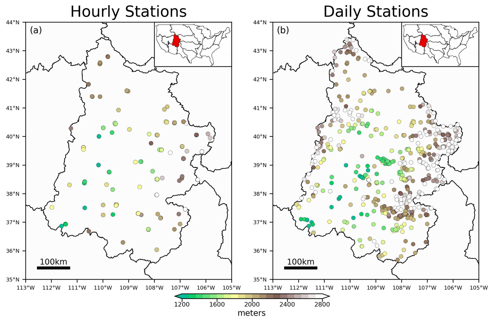
Figure 1 The hourly (a) and daily (b) distribution of stations across the Upper Colorado River Basin which are used in this study. The location of the study region is shown as the inset of the subplots alongside other large-scale hydrological basins across the contiguous United States. The color of the stations corresponds to the station elevation.

Daily measurements of precipitation are taken from the Global Historical Climatology Network – daily (GHCN-daily or GHCND) dataset (Menne et al., 2012). Most of these stations do not measure dew point temperature in-situ. Therefore, the ERA5 Reanalysis dataset (Hersbach et al., 2023) is used to provide dew point temperatures at the GHCND stations. For each GHCND station, the nearest ERA5 grid cell is found, and the corresponding time series of dew point temperatures are used for that station. This procedure is repeated for all of the GHCND stations in the UCRB. We use a common period of record for the hourly and daily data between 1 January 1951 through 31 December 2024. The distribution of the daily stations can be observed in Fig. 1b.

The hourly and daily datasets have been quality controlled to remove statistical outliers in both space (i.e., regional outliers) and time (i.e., temporal outliers). In our Supplement, we provide a comparison of the two quality-controlled datasets.

Throughout the paper, we use different data and/or indices. We begin by exploring the relationship between the raw (non-normalized) dew point temperature and raw precipitation data at the hourly resolution. Later in the paper, we rely on data at the station/month resolution, with one data point per station per month. For the hourly dataset, we find the maximum hourly precipitation amount at each station and for each month. For the duration of the paper, we refer to this value as Rx1hr. Also for the hourly dataset, we find for each station/month the concurrent dew point temperature which corresponds to the same time step as a given Rx1hr value. We also compute average monthly dew point temperature for each station/month. Likewise, for the daily dataset, we find the maximum daily precipitation amount at each station/month, referred to as Rx1day for the duration of the paper. Average monthly dew point temperatures are obtained from ERA5.

We additionally make use of normalized dew point temperature and precipitation data. Normalized anomalies of dew point temperature are computed as,

$$\begin{array}{}\text{(1)}& {\mathrm{DPT}}_{x,m,t}^{\ast }={\mathrm{DPT}}_{x,m,t}-{\stackrel{\mathrm{‾}}{\mathrm{DPT}}}_{x,m},\end{array}$$

where ${\mathrm{DPT}}_{x,m,t}$ is the average monthly dew point temperature (or concurrent dew point temperature) at station, x, month, m, and year, t, and ${\stackrel{\mathrm{‾}}{\mathrm{DPT}}}_{x,m}$ is the mean dew point temperature over the calibration time period at station, x, and month, m. Similarly, normalized anomalies of precipitation are computed as,

$$\begin{array}{}\text{(2)}& P_{x,m,t}^{\ast }={\displaystyle \frac{P_{x,m,t}}{{\stackrel{\mathrm{‾}}{P}}_{x,m}}}\times \mathrm{100},\end{array}$$

where $P_{x,m,t}$ is either Rx1hr or Rx1day at station, x, month, m, and year, t, and ${\stackrel{\mathrm{‾}}{P}}_{x,m}$ is the mean of the respective precipitation (either Rx1hr or Rx1day) time series over the calibration time period at station, x, and month, m. We only computed the normalized Rx1hr or Rx1day if the mean at station, x, and month, m, is greater than 1.0 mm. This helps us to avoid infinite or unrealistic values in the normalized data.

2.1 Evaluation Metrics Used for Validation

We evaluate model performance using the root mean squared error skill score (SS_RMSE). The skill score, SS_RMSE, is a function of the model and reference RMSE errors (RMSE_MOD and RMSE_CLIM, respectively). The RMSE_MOD is defined as,

$$\begin{array}{}\text{(3)}& {\mathrm{RMSE}}_{\mathrm{MOD}}=\sqrt{{\displaystyle \frac{\mathrm{1}}{n}}\sum _{i=\mathrm{1}}^n{\left(y_{\mathrm{mod},i}-y_{\mathrm{obs},i}\right)}^{\mathrm{2}}}.\end{array}$$

where y_obs and y_mod are the observed and the modeled precipitation values, respectively. Likewise, RMSE_CLIM, reflects the error associated with a baseline model which always assumes climatology (i.e., always assuming 100 % of normal, or equal to the climatological mean).

$$\begin{array}{}\text{(4)}& {\mathrm{RMSE}}_{\mathrm{CLIM}}=\sqrt{{\displaystyle \frac{\mathrm{1}}{n}}\sum _{i=\mathrm{1}}^n{\left(y_{\mathrm{clim},i}-y_{\mathrm{obs},i}\right)}^{\mathrm{2}}}.\end{array}$$

where y_clim contains the benchmark climatological precipitation values. The skill score can then be obtained as,

$$\begin{array}{}\text{(5)}& {\mathrm{SS}}_{\mathrm{RMSE}}=\mathrm{1}-{\displaystyle \frac{{\mathrm{RMSE}}_{\mathrm{MOD}}}{{\mathrm{RMSE}}_{\mathrm{CLIM}}}}.\end{array}$$

Skill scores of SS_RMSE above zero indicate that the model predictions are more skillful than climatology, while scores below zero indicate that the model is performing worse than climatology.

3 Methods

3.1 Common Challenges in Estimating P–T Scaling Rates

Our goal in this paper is to have a methodological approach that can more accurately estimate P–T scaling rates, and furthermore to use those estimates to make skillful predictions of extreme precipitation. We want to be able to estimate scaling rates with sufficient enough spatial and temporal resolution in order to say, for example, that a particular region (or station) in a given time of year (or month) can expect some average percentage increase in extreme precipitation provided that the region experiences, for example, +1 °C of warming in dew point temperature. The percentage increase per °C is our scaling rate and it will vary as a function of space (e.g., between stations or between grid cells) and time (e.g., between months of the year).

Without carefully managing the underlying data, one can incorrectly estimate and interpret P–T scaling rates. There are two primary concerns that must be addressed prior to using the data to estimate scaling rates:

1. Pooling raw (non-normalized) data of dew point temperatures and precipitation across multiple stations and/or months can lead to an inaccurate estimate of a scaling rate due to climatological differences that exist in both space (from station to station) and time (from month to month).

2. Data at hourly or daily resolutions cannot be assumed to be statistically independent in time.

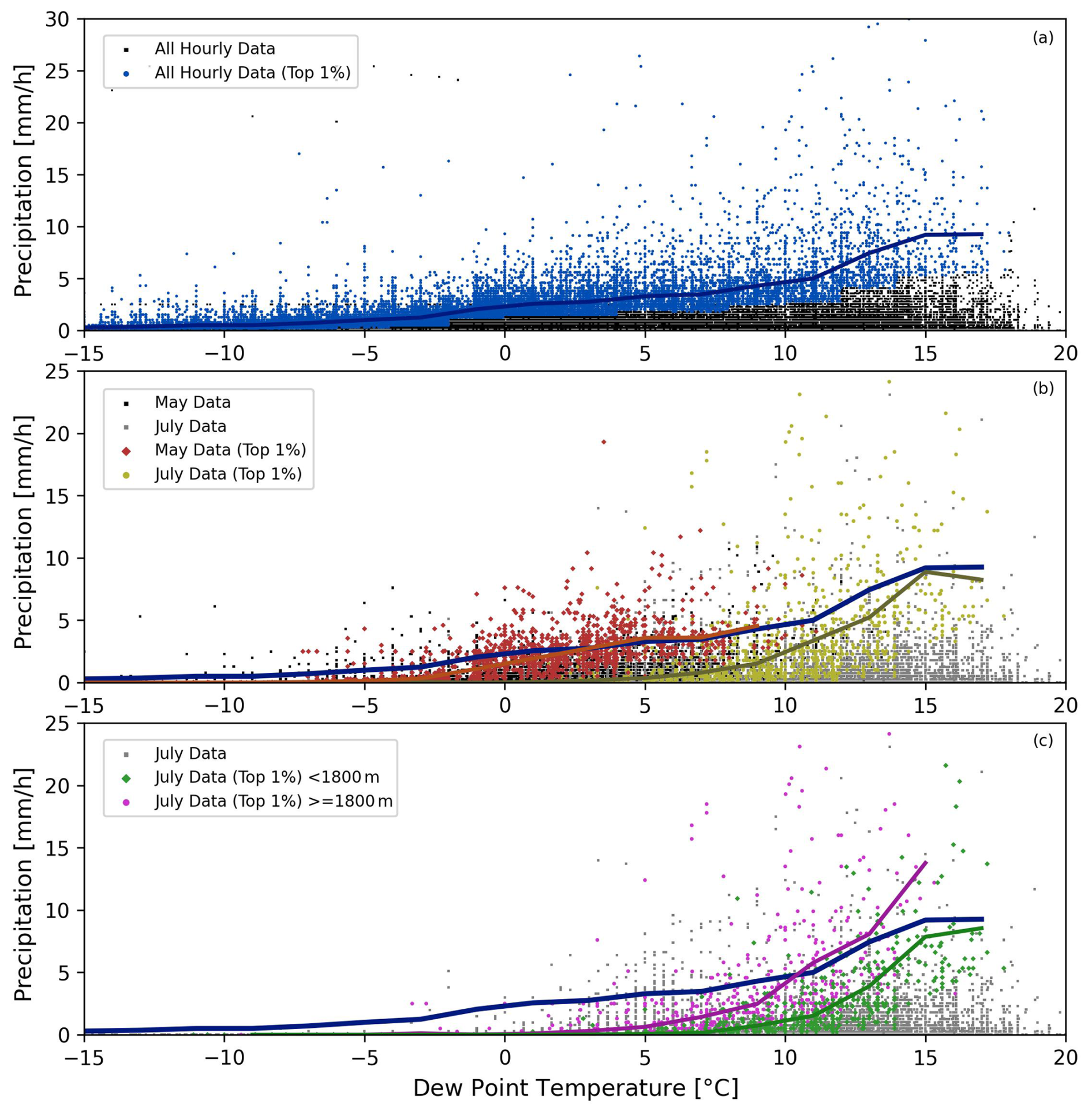
Figure 2 (a) All of the pairings of measured hourly precipitation along with the corresponding dew point temperature for the stations in the UCRB are plotted in the background as the black scatter points. The top 1 % of precipitation rates are plotted as the blue scatter points. The blue line is produced through the binning method, whereby the average of the top 1 % of precipitation rates are computed for each dew point temperature bin. Panels (b) and (c) use the top 1 % of precipitation, but where the top 1 % was found for each station and each month. Panel (b) shows the extreme precipitation for May (red points and the average is plotted as the red line) and for July (yellow points and line), using all of the stations in the UCRB. The average of the top 1 % from May and July can be contrasted to the blue line from panel (a). Panel (c) shows the difference between extreme precipitation in the month of July (i.e., top 1 %) using stations in the UCRB that are located below (green points and line) and above (magenta points and line) 1800 m in elevation.

In Fig. 2, we illustrate the first of the aforementioned challenges. While we primarily implement a quantile regression methodology throughout our paper, here we apply a binning method in order to more clearly show the problems of pooling raw (non-normalized) data from across space (e.g., different stations) and time (e.g., months). In Fig. 2a, we use all of the hourly data from all of the stations within the UCRB to look at pairs of dew point temperature and precipitation which are concurrent or collocated in time. The top 1 % of precipitation intensities are shown in blue for each dew point temperature bin (using a bin size of 2 °C and incrementing by 2 °C). One problem that can arise when finding the extreme precipitation values (e.g., the top 1 %), is that there can be certain months that are more extreme at the same dew point temperatures than other months. Similarly, there can be some stations that are more extreme at the same time of year, and at the same dew point temperatures, than other stations. We can test if this is the case by implementing the binning approach at the station/month level. So, for each station we can use all of the hourly data for a given month (all of the Julys for example). Then, we find the top 1 % of precipitation for each station/month at different dew point temperature bins. This gives us extreme precipitation amounts that are specific to every station, every month of the year, and every dew point temperature bin. We can then plot the influence of climatological differences across time as seen in Fig. 2b. Using these top 1 % of precipitation values that are derived at each station for each month, Fig. 2b illustrates how extreme precipitation differs between the month of May and the month of July. Within the same dew point temperature bin, for example, which is centered at 5 °C (between 4 and 6 °C), extreme precipitation is dramatically different between these two months. For the month of May, the average precipitation that falls in the top 1 % of this bin is 3.60 mm h⁻¹ (with 171 samples). In contrast, the average precipitation in the top 1 % of the same bin is 0.36 mm h⁻¹ for the month of July (with 252 samples). The average extreme precipitation in May at a dew point temperature of 5 °C is 10 times that of July (the distributions are statistically significantly different with a p < 0.01). Next, let us focus on the influence of climatological differences across space. In Fig. 2c, the top 1 % of precipitation values are plotted for the month of July, but the stations are split by elevation as being either below or above 1800 m. Again, we can use a bin, such as the one centered at 11 °C, to observe that even at the same dew point temperature and at the same time of year, certain stations exhibit more extreme precipitation than others. For stations above 1800 m, the average precipitation that falls in the top 1 % of this bin is 5.83 mm h⁻¹ (with 163 samples). In contrast, the average precipitation in the top 1 % of the same bin is 1.49 mm h⁻¹ for the stations below 1800 m (with 118 samples). For the month of July, the average extreme precipitation for stations above 1800 m and with a dew point temperature of 11 °C is 4 times that of stations below 1800 m (p < 0.01). These climatological differences in both time and space adversely influence the sampling frequencies, when applying a binning method or quantile regression using pooled raw (non-normalized) data. Some months will be sampled at higher rates, such as May as opposed to July. Similarly, some stations will be sampled at higher rates, such as stations above 1800 m in elevation as opposed to stations below 1800 m. This influence leads to inconsistent sampling, where some stations, at some times of year, might never be sampled from, while others are sampled at greater than our specified quantile (e.g., 1 %). As a result, we would estimate a scaling rate using data that more heavily weights certain stations at certain times of year. By sampling the top 1 % more heavily from stations above 1800 m in May versus stations below 1800 m in July, for example, we end up overfitting or underfitting the scaling rate to data at certain locations and at certain times of the year.

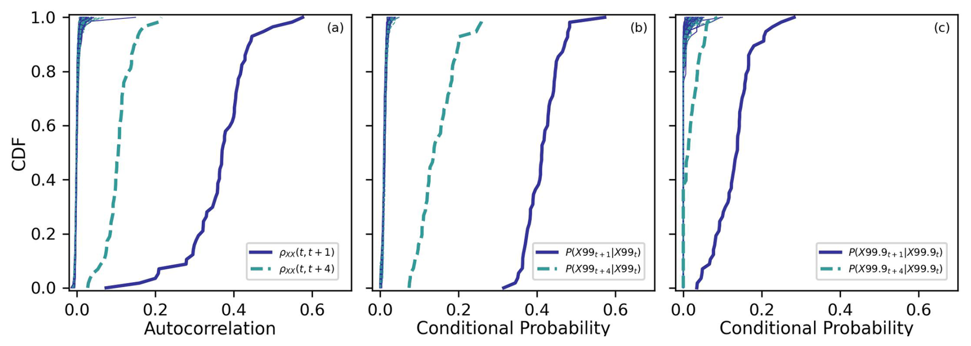
Figure 3 (a) Empirical cumulative distribution functions (CDFs) of the lagged-1 and lagged-4 h autocorrelations from the stations in the UCRB are plotted as the blue solid and light blue dashed lines, respectively. CDFs from randomly generated time series are seen as the thin lines on the left. (b) Empirical CDFs of the lagged-1 and lagged-4 h conditional probabilities are shown for extreme precipitation. For each station, the probability of an extreme precipitation (in this panel, this is the top 1 %) event is followed by another extreme precipitation event 1 or 4 h later are plotted as the blue solid and light blue dashed lines, respectively. (c) Same as panel (b) except using the top 0.1 % instead of top 1 % of precipitation.

Moving to the next issue, the data used in Fig. 2 cannot be considered to be statistically independent in time. The data from one time step at a given station is not independent of the data at the next time step at the same station. Due to this lack of data independence, the effective sample sizes are actually much less than what is suggested in Fig. 2. We can show the issue with statistical independence in two different ways using the hourly precipitation data. First, we can compute the temporal autocorrelation of the data for each station. We do this using two different lagged time steps, where we compute lagged-1 and lagged-4 h autocorrelations. The lagged autocorrelations for all of the stations in the UCRB, which have been sorted, are plotted as empirical cumulative distribution functions (CDFs) in Fig. 3a as the thicker lines on the right. Next, we test whether these distributions are statistically significantly greater (or shifted to the right) from what we would expect by chance. We generate 1000 randomly sampled time series for all stations. At each station, bootstrapping is used to randomly create a time series of data points drawing from the empirical distribution of data points from that station. The CDFs of the stations from these randomly generated time series are seen as the thinner lines on the left side of Fig. 3a. Precipitation data which is separated by less than 4 h cannot be considered to be statistically independent of one another (p < 0.01). In Fig. 3a, all of the hourly precipitation data is used, including zeros, and as a result it does not provide information specifically related to the independence of extreme precipitation events. Therefore, we can next compute conditional probabilities for extreme precipitation values. Let us first focus on precipitation events which fall in the top 1 %. For each station, we find all of the cases where if precipitation at hour, t, was in the top 1 %, then what was the probability that hour, t+1, or hour, t+4, was also in the top 1 %. The thicker lines in Fig. 3b show the CDFs of these two conditional probabilities across the stations. Again, we find the conditional probabilities of the extreme precipitation data to be greater than randomly generated data (p < 0.01). One can note that the lagged-1 conditional probability of the data is approximately 40 times what we would expect by chance (compare 0.4 as the approximate average of the thick blue line versus 0.01 as expected by chance). Figure 3c shows the results using the top 0.1 % of precipitation, where again we find that extreme precipitation events cannot be considered independent of one another over time periods of less than 4 h. As one continues to increase the duration of time between extreme precipitation events, beyond 4 h for example, then those events begin to exhibit more statistical independence from one another. When it comes to conditional probabilities, we find for data in the UCRB, that the data on average approaches statistical independence for events separated by approximately 12 h for the top 0.1 % and approximately 24 h for the top 1 %.

Figure 4 (a) Normalized concurrent dew point temperature anomalies are plotted along with normalized Rx1hr precipitation. (b) Normalized monthly average dew point temperature anomalies are plotted along with normalized Rx1hr precipitation. The correlation coefficients between the data points in each panel are seen in the upper-right corners.

There are two other notable points to discuss here. First, when applying a binning method, one must additionally take care with respect to the various sample sizes across different bins. For this reason, we implement a methodology which fits an exponential regression model to the monthly precipitation maxima Rx1hr and Rx1day. Second, there is the issue of whether or not to use dew point temperature data which is concurrent in time with the Rx1hr or Rx1day precipitation value. Our primary goal in this paper is to devise an effective method of estimating scaling rates where they can be used to predict expected changes in extreme precipitation given changes in dew point temperatures. Estimating concurrent relationships between dew point temperature and extreme precipitation for a region in a given season is often done with knowledge of when exactly the extreme precipitation events have already taken place. In that case, the dew point temperature is found corresponding to the same hour of the extreme precipitation amount that fell in the top specified quantile, such as 1 %. However, if we have a projected change in our hourly dew point temperature distribution without prior knowledge of when the most extreme precipitation event happened, we cannot say ahead of time at which hour, or dew point temperature, the most extreme precipitation event will take place. It is possible that the most extreme hourly precipitation rate can be concurrent with any of the dew point temperature values within the distribution from that station/month. Considering a distribution of 744 hourly values of dew point temperature at a given station in July, which of these hourly dew point temperatures do we use as our predictor of extreme precipitation? We cannot know exactly which hourly dew point temperature value corresponds with the extreme precipitation amount, and therefore our predictor can ultimately be thought of as a shift in the mean of the distribution over the month. In fact, using monthly averages of dew point temperatures instead of concurrent dew point temperatures can even enhance the statistical relationship, or predictive power, between our predictor and our predictand. Both Zhang et al. (2017) and Marra et al. (2024) have previously explored using predictor data which is not concurrent with extreme precipitation. Zhang et al. (2017) used only wet-days to compute an average seasonal dew point temperature, while Marra et al. (2024) used average daily temperatures. Figure 4a plots the normalized concurrent dew point temperature anomalies along with normalized Rx1hr precipitation. Figure 4b plots the normalized monthly average dew point temperature anomalies along with normalized Rx1hr precipitation. One can observe in the case of the UCRB, that there is a stronger statistical relationship (indicated by the difference in correlation coefficients between Fig. 4a and b) between the monthly average dew point temperature and Rx1hr than the concurrent hourly dew point temperature. For these reasons, we use the monthly average dew point temperatures as our predictor of Rx1hr and Rx1day precipitation.

3.2 Proposed Approach for Estimating P–T Scaling Rates

In the prior section, we pointed out a number of problems that can adversely influence our estimation of P–T scaling rates. For our modeling approach, we use data at the resolution of one value per station per month. This gives us data that exhibits a greater degree of statistical independence than data at the hourly or daily resolution. Next, as we illustrated in Fig. 2, raw or non-normalized can lead to over- or undersampling certain stations and/or months. This is due to the fact that there are climatological differences in time and space, and some stations in some months will on average have more extreme precipitation events than other stations and/or months, even at the same dew point temperature. By normalizing the data, we provide a more homogeneous framework for dealing with different types of precipitation (Berg and Haerter, 2013; Molnar et al., 2015). It is therefore advisable to normalize the data, following Eqs. (1) and (2), prior to estimating any P–T scaling rates.

Our approach uses an exponential regression model. Previously, we have shown some of the problems that can arise when using pooled, non-normalized data and which also lacks statistical independence. We therefore fit a exponential regression model between monthly average dew point temperatures and Rx1hr, or Rx1day if we are using the daily dataset. The model fit minimizes the least-squares over the following exponential function:

$$\begin{array}{}\text{(6)}& y=a\cdot b^x,\end{array}$$

where x contains monthly-averaged dew point temperature anomalies, from the array DPT^∗ (or DPT if using non-normalized data), a is a multiplicative offset, b is interpreted as our scaling rate, and y would be either the normalized (or non-normalized) values from Rx1hr or Rx1day. The model fit is performed using the optimize function contained in Python's Scipy package.

3.3 Predicting Extreme Precipitation

Consider a synthetic example where we were to fit the model to normalized data from Eqs. (1) and (2). Given that the model is fit to the normalized data, the value of a would approximately equal 100 (which is 100 % of normal, this value ultimately depends on the distribution and the skewness of the data), and consider the value of b is found to be 1.08 (i.e., the scaling rate is 8 % °C⁻¹). With this example, and given a +2 °C average monthly dew point temperature anomaly, we would predict Rx1hr (or Rx1day) to be 116.6 % of normal.

Predictions of Rx1hr and Rx1day are performed using leave-one-year-out cross validation over the period 1951–2024. For the daily dataset, which has sufficient data coverage throughout the period of record, we additionally perform a two-fold cross validation with the data being split into two equal time periods, with the first period being 1951–1987 and the second period being 1988–2024. We have four models that we use to make predictions and evaluate model performance. These are in increasing complexity, (1) always assuming 100 % of normal, (2) fitting the exponential model from Eq. (6) to the normalized data and always assuming a C–C scaling rate of 7 % °C⁻¹ (i.e., this fits Eq. (6) to solve for a when b is fixed to a value of 1.07), (3) fitting the exponential model from Eq. (6) to the raw (non-normalized) data, and (4) fitting the exponential model from Eq. (6) to the normalized data. Through this procedure of implementing different modeling approaches with different data, we can determine which approach provides the best performance. With regard to the fourth model, we also investigated fitting the exponential model to standardized anomalies (i.e., z-scores, or standard deviations from the mean). Using standardized data in the model produced very similar results to what we found using the normalized data (not shown). However, our proposed approach of using normalized data benefits from having less complexity and provides more easily interpretable scaling rates expressed as % °C⁻¹.

We can use the fourth model (i.e., fitting Eq. 6 to normalized data) from the prior paragraph to briefly outline our procedure to produce leave-one-year-out cross-validated predictions of Rx1hr. For each year, the average monthly dew point temperatures (DPT^∗ from Eq. 1) and Rx1hr precipitation (P^∗ from Eq. 2) are computed using only the calibration years which exclude the year for which we are going to make model predictions of the anomalous Rx1hr. Likewise, the model is fit using Eq. (6) to the data from the calibration years, and model predictions are produced for the given validation year. For each validation year in turn, we additionally retain the observed precipitation anomalies computed using mean values of Rx1hr calculated from the current set of calibration years. These observed anomalies will be used in our model evaluation. Then, we step to the next year until we have covered the entire time period, 1951–2024. For the two-fold cross validation scenario, the average monthly dew point temperatures (DPT^∗ from Eq. 1) and Rx1day precipitation (P^∗ from Eq. 2) are first computed using the calibration years 1951–1987. The model is fit using Eq. (6) to the data from these calibration years, and predictions are produced for the validation period 1988–2024. Then, data from the years 1988–2024 is used for calibration, and the years 1951–1987 are predicted.

Each of the last three models (models 2–4 listed above), use a range of spatial and temporal extents over which to fit the model and make predictions. This is done to observe if, and to what extent, the pooling of data across different stations and/or months can improve the estimated P–T scaling rates and the associated predictions. We use four spatial extents where we pool data from: (1) only the station being predicted, (2) stations within a 50 km radius of the station being predicted, (3) stations within a 100 km radius of the station being predicted, and (4) all of the stations that fall within the entire region (in our case, the UCRB). Similarly, we use four temporal extents where we pool data from: (1) solely the month being predicted (i.e., 1-month window), (2) a 3-month window centered about the month being predicted, (3) a 5-month window centered about the month being predicted, and (4) all 12 calendar months.

Figure 5 Comparing the model fit using non-normalized versus normalized data. The data points correspond to all of the stations in the UCRB and using a 3-month window corresponding to the winter and summer seasons. Panel (a) plots all of non-normalized values of average monthly dew point temperature plotted against Rx1hr for the December–January–February winter season. The model fit using Eq. (6) is plotted as the black line. Panel (b) is the same as panel (a) except using normalized data. Panels (c) and (d) are the same as panels (a) and (b) except for the June–July–August summer months. Panels (e)–(h) are the same as panels (a)–(d) except now using Rx1day instead of Rx1hr.

In Fig. 5, we can observe the process of model fitting to non-normalized versus normalized data. In these cases from Fig. 5, we use all of the stations in the UCRB (i.e., spatial extent number 4), and a 3-month temporal window (i.e., temporal extent number 2). The top row of subplots (Fig. 5a–d) show the relationship between either non-normalized, or normalized, average monthly dew point temperatures and Rx1hr precipitation. This is shown using the data from the winter (December–January–February) and summer (June–July–August) seasons. The bottom row shows the same as the top row, except using daily data (i.e., Rx1day). One can observe substantial differences in model fitting when we are controlling for climatological differences (using normalized data) and when we are not (using non-normalized data). A prime example of this is illustrated by Fig. 5e and f. The same data, with the same number of data points, is used in both of these cases. However, the values in Fig. 5f have been normalized using Eqs. (1) and (2). Without applying this normalization, we miss the fact that stations at higher elevations climatologically experience lower dew point temperatures while also experiencing climatologically greater Rx1day precipitation. We find that the elevation of the daily stations is correlated with the values of average Rx1day over the time period during the winter season with a correlation coefficient of 0.69, with the average Rx1day for stations centered about 3000 m in elevation (between 2750–3250) being more than double that of stations centered about 1500 m (between 1250–1750). Without controlling for climatological differences in space, which is the case in Fig. 5e, we end up conflating these climatological differences with the scaling rate. After normalization, we observe a positive scaling rate as seen in Fig. 5f. To produce the different sets of model predictions of Rx1hr and Rx1day, the procedure outlined in Fig. 5 is performed using a cross-validated framework, for the C–C, non-normalized, and normalized models. In addition, for each model case, we iterate through the four spatial and temporal extents. Model predictions which rely on the raw, non-normalized data initially provide predictions as non-normalized values of Rx1hr precipitation (i.e., mm per hour). These modeled values are subsequently normalized using Eq. (2) prior to model evaluation.

4 Results

4.1 Evaluating Model Performance

The underlying empirical-statistical relationship between the normalized average monthly dew point temperature and normalized Rx1hr is plotted for all stations and all months in Fig. 6a. In Fig. 6b, the individual leave-one-year-out cross-validated predictions of Rx1hr are plotted versus observed Rx1hr. The predicted Rx1hr in Fig. 6b are produced using the normalized data model with a spatial extent of 100 km and a 3-month temporal window. While individual predictions of Rx1hr and Rx1day precipitation are produced, as depicted in Fig. 6b, the individual values themselves exhibit large fluctuations due to natural variability. This is due to the fact that we are solely conditioning changes in extreme precipitation on changes in dew point temperature. Given the large variability of the individual values themselves, we evaluate model performance as the average change in Rx1hr or Rx1day precipitation given specified average monthly dew point temperature anomalies ranging between −3 °C below normal to +3 °C above normal. At each dew point temperature anomaly, we compute the mean extreme precipitation anomaly centered about that dew point temperature anomaly. We use a 1 °C window, with 1 °C increments, and find the modeled and observed extreme precipitation distributions corresponding to dew point temperature anomalies −3, −2, −1, 0, +1, +2, and +3 °C. Model performance evaluates how well the predicted mean shifts in the normalized extreme precipitation align with the observed mean shifts. In Fig. 6c, we can look more specifically at the Rx1hr anomalies for each of these dew point temperature anomalies using the summer months June–July–August. The orange points show, for example, the Rx1hr values that fall within the one degree window centered about a +1 °C anomaly. The empirical CDFs corresponding to different dew point temperature anomalies, along with the means of those distributions, are shown in Fig. 6d. This provides us with seven mean observed Rx1hr precipitation anomalies (as % of normal) as a function of the seven dew point temperature anomalies for the 3-month window centered about July. We can similarly compute the seven mean predicted Rx1hr precipitation anomalies for this case (not shown). We then perform the same procedure for all 12 months of the year. By doing that, we have 84 predicted versus observed mean Rx1hr anomalies for the different dew point temperatures and for the different months of the year. These values are plotted in Fig. 6e. In the case of this model (i.e., normalized data with 100 km spatial extent and a 3-month temporal window), the RMSE of the model is 6.4. The benchmark model RMSE, which always assumes climatology (always 100 % of normal) is 21.9. Using Eq. (5), we find our SS_RMSE is 0.71. The same procedure is performed separately for Rx1hr and Rx1day using predictions from the C–C model, the non-normalized model, and the normalized model, and where in each model case the four different spatial and temporal extents were implemented.

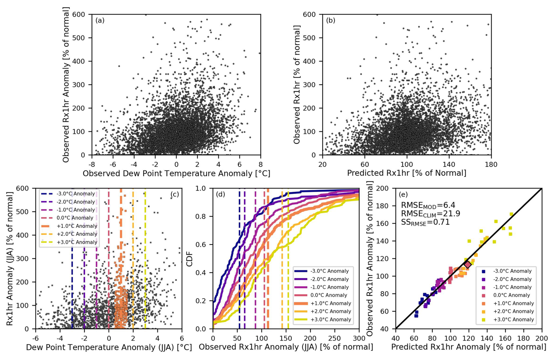
Figure 6 Panel (a) plots the relationship between the normalized average monthly dew point temperature (our predictor) and normalized Rx1hr (our predictand) for all stations and all months. Panel (b) plots the individual cross-validated predictions of Rx1hr versus observed Rx1hr using the normalized data model with a spatial extent of 100 km and a 3-month temporal window. In panel (a), our predictor corresponds to the x-axis, while in panel (b) our cross-validated predictions corresponds to the x-axis. The values along the y-axis of both panels (a) and (b) are the observed Rx1hr anomalies and they are the same in each panel. (c) Dashed lines show the different dew point temperature anomalies over which the mean predicted versus observed Rx1hr anomalies are evaluated. This panel shows the observed data for the 3-month window centered about July. The orange points show the distribution of Rx1hr along the y-axis corresponding to a +1 °C dew point temperature anomaly. (d) The empirical CDFs, for the different distributions corresponding to different temperature anomalies, are plotted as the lines. The dashed lines show the mean shift of the observed distributions. The thicker orange dashed line shows along the x-axis the observed mean shift in Rx1hr (i.e., average of orange points from panel (d)) given the example case of a +1 °C dew point temperature anomaly. Panel (e) plots all of the seven predicted mean versus observed mean Rx1hr precipitation anomalies for the 12 months of the year, giving us 84 points. The larger orange diamond corresponds to the example case illustrated in panels (d) and (e).

4.2 Model Performance

In Fig. 7a, we show the range of model skills, SS_RMSE, using leave-one-year-out cross validation for the 16 possible iterations of spatial-temporal extents using the C–C model, the non-normalized model, and the normalized model. Figure 7a plots the skills of the cross-validated Rx1hr predictions for the three different models. In the case of Rx1hr, the best obtained skill score is 0.45 for the C–C model, 0.66 for the non-normalized model, and 0.71 for the normalized model. The dotted black line in Fig. 7a are the skill scores obtained from 1000 randomly generated predictions (or simulations), where each individual set of predictions can be analogously compared or contrasted to the points along the x-axis in Fig. 6b, for example. These random predictions follow the same modeling framework used by the other models, especially as it comes to computing anomalous values through cross-validation, except we do not perform any actual model fitting. Instead, for each year and for one set of predictions, we randomly select a year from the calibration period to be used as the predicted values. Through this process, we successfully preserve the spatio-temporal covariance of the observational data in our randomized simulations. We can then test how skillfully one can randomly predict Rx1hr (or Rx1day), when the randomized predictions exhibit the same spatio-temporal covariance structure as the underlying data. The best obtained skill of the 1000 randomly generated predictions is 0.09. As a result, the best performing skill scores from all three models are found to be statistically significantly better than both climatology and what we would expect by chance (p < 0.01). If it is not already clear, we want to stress at this point, that all of the models, whether a randomized set of predictions, the C–C model, the non-normalized model, or the normalized model, all have access to exactly the same data to produce the cross-validated predictions. The models only differ in how they make use the data (e.g., non-normalized versus normalized) and what assumptions are made (e.g., C–C always assumes 7 % °C⁻¹). In Fig. 7b–d, we observe in what combinations of spatial and temporal extents each respective model sees its maximum skill score. We observe fairly uniform positive skill for the C–C model in Fig. 7b, with small variations present due to a changing sample size between different spatial and temporal extents. For the non-normalized model (Fig. 7c), its optimal skill is found to correspond to using the 50 km spatial extent along with the 1-month temporal window. One can clearly observe the skill decrease for the non-normalized model as the data is pooled from further away in both space and time. When pooling data from the entire UCRB region and using all of the data throughout the year (i.e., the bottom-right grid cell in Fig. 7c), the skill is less than half of what it is in its optimal case, or 0.30 versus 0.66. This is primarily due to the fact that the non-normalized model includes pooled data with very different climatologies in time and space. Another reason is that we are mixing different scaling rates across time and space, where each station can be considered to have a certain scaling rate for a given time of the year, such as July. For this second reason, we also see a decrease in skill for the normalized model when pooling data from the largest spatial and temporal extents (see Fig. 7d). However, the normalized model is able to leverage data from larger spatial and temporal extents in order to improve the skill with respect to using non-normalized data. The maximum skill of the normalized model is 0.71 and corresponds to the grid cell bounded by the yellow box (this case was also illustrated in Fig. 6b and e). A t-test between the model errors (as depicted about the one-to-one line, for example, in Fig. 6e) that are associated with the optimal skill scores between the non-normalized and normalized models show the normalized model provides statistically significantly better skill than the non-normalized model (p < 0.01). Figure 7e–h show the same as Fig. 7a–d except evaluating the model performance in predicting Rx1day precipitation. Generally, the results follow the same pattern with the optimal model skills for the three models being 0.63, 0.74, and 0.81, respectively. What is apparent now, is that the skill of the non-normalized model immediately begins to degrade as any amount of data pooling is performed. The non-normalized model provides the best results when the calibration data is used from only the station and month being predicted. The drop off in skill for the non-normalized model, which uses pooled data, is even more profound that what we observed for Rx1hr (Fig. 7c). Using data with a 100 km spatial extent and a 5-month temporal window, for example, gives worse skill than climatology (see the corresponding light red grid cell in Fig. 7g). Please refer again to Fig. 5e–h, to observe the impact that controlling for climatological differences in space and time can have on model fitting. The maximum skill of the normalized model is again bounded by the yellow box in Fig. 7h, and this skill is again found to be statistically significantly better than the optimal non-normalized skill score (p < 0.01).

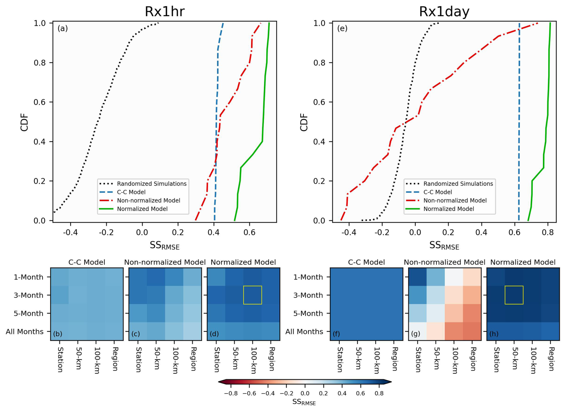
Figure 7 Panel (a) plots the skills as empirical CDFs of the leave-one-year-out cross-validated predictions of Rx1hr for the three different models: C–C, non-normalized, and normalized. The CDFs are comprised of the skills from the different possible iterations of the spatial and temporal extents. Additionally, the CDF of 1000 randomized simulations is shown as the black dotted line. Panels (b), (c), and (d) show the skill scores as a function of model (corresponding to panel title), spatial extent (x-axis), and temporal extent (y-axis). The maximum skill achieved is highlighted with the bounded yellow box. Panels (e)–(h) are the same as panels (a)–(d), except showing the skills in predicting Rx1day.

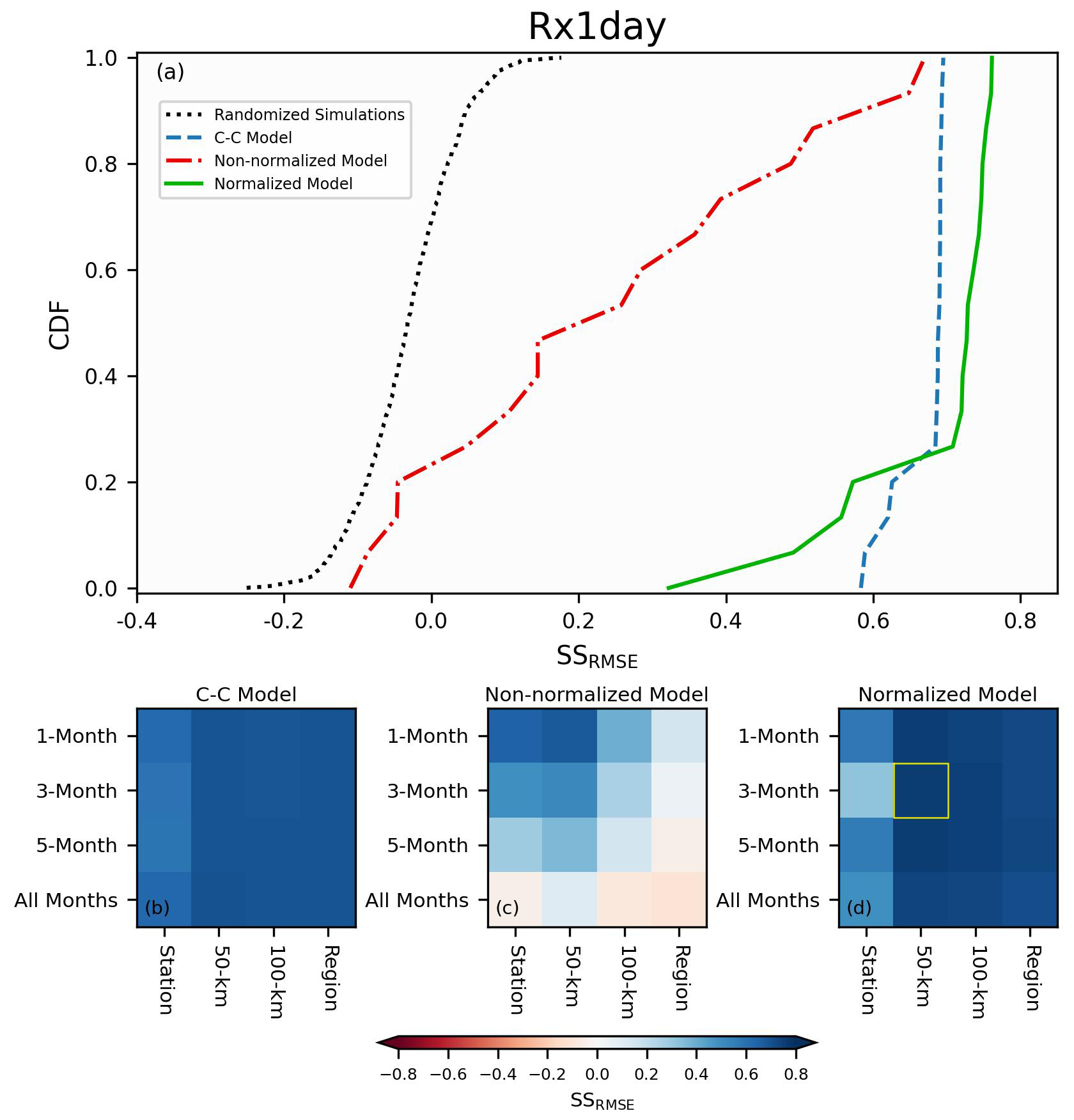
Figure 8 Panel (a) plots the skills as empirical CDFs of the two-fold cross-validated predictions of Rx1day for the three different models: C–C, non-normalized, and normalized. The CDFs are comprised of the skills from the different possible iterations of the spatial and temporal extents. Additionally, the CDF of 1000 randomized simulations is shown as the black dotted line. Panels (b), (c), and (d) show the skill scores as a function of model (corresponding to panel title), spatial extent (x-axis), and temporal extent (y-axis). The maximum skill achieved is highlighted with the bounded yellow box.

Figure 8 shows the same results as Fig. 7, except we now predict Rx1day using two-fold cross validation. In this case of the two-fold cross validation, the best obtained skill score is 0.68 for the C–C model, 0.66 for the non-normalized model, and 0.76 for the normalized model. These values are quite similar to what we obtained and plotted Fig. 7e–h for the leave-one-year-out cross validation, especially seen in the fact that we can still leverage normalized data to improve the predictions of Rx1day precipitation. This result provides a better understanding as to how well the methodology can apply in the context of a changing climate. With the results from Fig. 7 alone, one might misinterpret that the skill we observe is entangled with the trends in the underlying data. However, the results from Fig. 8 show that is not the case, and that the method can successfully produce skillful predictions over multi-decadal lengths of time.

4.3 Estimated Scaling Rates

With regard to the models that we evaluated, our model which uses normalized data is found to provide the best cross-validated skill. For Rx1hr, the best model performance was using a 100 km spatial window and a 3-month temporal window. While for Rx1day, the best model performance was using a 50 km spatial window and a 3-month temporal window. We then use the normalized data with these respective model parameters governing the spatial and temporal extents to estimate the scaling rates for each station and each month of the year. The top row of panels in Fig. 9a plots the scaling rates of Rx1hr at each station for each month of the year. In Fig. 9b, we plot the scaling rates of Rx1day at each station for each month of the year. In Fig. 9c, a boxplot shows the distribution of scaling rates for both Rx1hr and Rx1day for each month of the year. The median scaling rates for both Rx1hr and Rx1day, in the winter months, exhibit sub C–C (i.e., < 7 % °C⁻¹). Additionally, the wintertime Rx1day is found to scale more strongly, on average, than Rx1hr. On the other hand, the median scaling rates in the summer months exhibit super C–C (> 7 % °C⁻¹). In contrast to the winter, the summertime Rx1hr scales more strongly, on average, than Rx1day. Some stations in the summer months exhibit scaling rates that are approximately triple the C–C scaling rate. The median P–T scaling rates for Rx1hr, as a function of month, range between 4.6 % °C⁻¹ for January and 17.0 % °C⁻¹ for June. While for Rx1day, the scaling rates range between 5.2 % °C⁻¹ in December to 12.9 % °C⁻¹ in June.

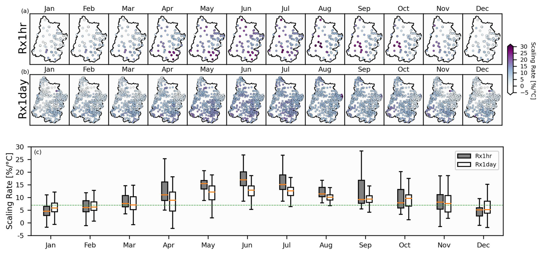
Figure 9 The top row (a) plots the scaling rates of Rx1hr at each station for each month of the year. (b) Same as panel (a) except for Rx1day. Panel (c) uses a boxplot to show the distribution of the scaling rates as a function of Rx1hr or Rx1day along with the month of the year. In panel (c), each box, median, and whiskers are constructed using the scaling rates from all of the stations in the UCRB corresponding to that month and either Rx1hr or Rx1day. The gray boxplot for July, as an example, is constructed using the scaling rates from the stations in the “Jul” panel in panel (a).

5 Conclusions

Using point-scale station data from the Upper Colorado River Basin, this study begins by illustrating some common challenges in estimating P–T scaling rates. Our aim, herein, has not been to provide a comprehensive overview of every existing methodology related to P–T scaling rates, but rather to focus on some of the prevailing challenges confronting scaling rate estimation along with some proposed solutions. We find that there are two primary challenges that require careful consideration prior to implementing any estimation of scaling rates. These are: (1) using pooled data across multiple stations and/or months, without normalization, can lead to inaccurately estimating the scaling rate due to climatological differences that exist in both space (from station to station) and time (from month to month), and (2) the statistical independence of the data in time.

Drawing upon prior research (Wasko and Sharma, 2014; Zhang et al., 2017; Molnar et al., 2015; Visser et al., 2021), we propose a strategy which reduces the impact of these two problems. Our approach relies on using average monthly dew point temperatures as a predictor of Rx1hr and Rx1day precipitation. We then implement a regression model which fits an exponential function between these two variables for a multitude of cases. For each precipitation variable, such as Rx1hr, we make cross-validated predictions using three models and compare the model error with respect to if we had always assumed climatology. The three models are: (1) always assuming C–C scaling, (2) using the data without normalization, and (3) using the data with normalization. Additionally, we make the cross-validated predictions using a range of spatial and temporal extents. We find that both the non-normalized and normalized models are capable of providing better predictions of Rx1hr and Rx1day than either relying on climatology or the C–C scaling rate. Furthermore, the normalized data model is able to more effectively leverage pooled data when compared to the non-normalized data model. As a result, the best model performances are obtained through the normalized model for both Rx1hr and Rx1day. In the case of the UCRB, we find optimal performance using normalized data along with a 3-month temporal window and approximately a 50 to 100 km spatial extent. Regarding the non-normalized model, it is clear that the best performance is achieved when using very narrow windows of spatial and temporal extents, such as using only data from the station itself for a given month (i.e., which uses all the years for that station and that month). Given the relatively sparse hourly dataset, we found the non-normalized model is able to leverage data from adjacent stations up to 50 km away, but the performance degrades with attempts to pool data from further away in space or time. For the daily dataset, which has increased data coverage, the best performance of the non-normalized model is found without implementing any data pooling. After normalizing the data, however, we can more effectively pool temporally and spatially adjacent data, and as a result we improve our estimates of our scaling rates and the associated predictions of precipitation extremes. We should note that our methodology has assumed that the scaling rates are stationary over our period of record, which appears to be a good assumption if we compare the results of leave-one-year-out and two-fold cross validation cases for Rx1day. Our paper's focus has been to illustrate the value of normalizing data in an effort to more accurately estimate P–T scaling rates. However, future research can focus on investigating whether or not scaling rates can be considered stationary. Another issue worth mentioning is the potential impact of the measurement precision of the precipitation data (Ali et al., 2022). In this study, we used data at a measurement precision of 0.1 mm. However, we did additionally try rounding our precipitation data to the nearest 1.0 mm prior to normalization, and this was not found to noticeably impact our results. Lastly, while our proposed method is capable of modeling either positive and negative scaling rates, it is not capable of handling cases where the normalized data experiences a transition between positive to negative scaling, or vice-versa.

Using our best performing model, which uses normalized data pooled from 100 km or 50 km (for Rx1hr and Rx1day, respectively) and a 3-month window, we finally show the scaling rates at each station for each month of the year. The scaling rates associated with daily extreme precipitation, Rx1day, are found to exhibit less variability throughout the year than scaling rates associated with hourly extreme precipitation, Rx1hr. The median of the June scaling rates, for Rx1hr, is more than triple the median of the January scaling rates. Substantial variability is seen in the scaling rates across both space and time, and as a result it is advisable that one estimates a unique P–T scaling rate at every given station (or grid cell if using gridded data) and for every given time of year (such as a month).

In this study, we have achieved skillful cross-validated predictions of extreme Rx1hr and Rx1day precipitation in the UCRB by fitting an exponential model to normalized data. By applying this methodology to other regions of the world, we can gain a more detailed and comprehensive understanding of how P–T scaling rates vary across space and time. This information is essential in our efforts to improve our preparedness regarding extreme precipitation.