Different tracer, different bias: using radon to reveal flow paths beyond the Window of Detection

Slug tracer experiments have greatly advanced our understanding of solute transport in streams. Breakthrough curves (BTCs) from these experiments are biased toward faster flow paths, highlighting the need for alternative tracers to cover longer timescales. The radioactive tracer radon (²²²Rn) is increasingly used to quantify transit times in subsurface transient storage zones, capturing durations of up to 21 d. However, it remains unclear whether calibrating transient storage models (TSMs) with radon yields longer subsurface timescales of transit times than calibrating them with slug tracers such as sodium chloride (NaCl). To address this, we conducted radon measurements and NaCl slug tracer experiments in Oak Creek (Oregon, USA) and jointly and individually calibrated TSM parameters with both tracers. We applied parameter identifiability analysis and used information theory to evaluate how the two tracers constrain model parameters. Our results show that TSM calibration with both radon and chloride increases parameter information compared to TSM calibration with either tracer alone. This suggests that incorporating radon into calibration improves estimates of solute transport in future studies. However, when calibrating the TSM with only radon measurements, all resulting parameters of the TSM were non-identifiable. This non-identifiability arises because radon activity in streams remains at steady-state and is highly sensitive to the location and amount of groundwater inflow, as well as contributions of flow paths from subsurface transient storage zones. As a result, radon measurements are biased toward longer-timescale flow paths, limiting their applicability to uniquely constrain solute transport parameters in TSM calibration without complementary slug tracers.

1 Introduction

The time a water parcel spends in river corridors is a key variable controlling biogeochemical processes and the ecological functioning of streams (Harvey and Gooseff, 2015; Ward and Packman, 2019). In environmental systems, the combined distribution of these timescales for many parcels of water is called transit time distributions (TTDs). Empirical studies of TTDs in streams typically rely on solute tracer experiments (e.g., Stream Solute Workshop, 1990), which involve releasing a known mass of solute tracer into the stream and measuring its concentration over time, i.e., the breakthrough curve (BTC), at a downstream location (Day, 1976). Despite their widespread use, solute tracer experiments are biased toward measuring faster flow paths within TTDs due to the “window of detection” (WoD). The WoD refers to the longest temporal scale of tracer-labelled flow paths that contribute to measurable tracer concentrations distinguishable from the background concentration (Harvey et al., 1996; Wagner and Harvey, 1997; Ward et al., 2023), ultimately defining the longest timescales that can be observed in a given study. Despite decades of research (Harvey and Bencala, 1993; Wagner and Harvey, 1997), measuring flow paths with timescales beyond the WoD remains challenging. This challenge leaves critical gaps in our understanding of solute transport in streams when relying solely on BTCs and underscores the need for new approaches to capture these overlooked timescales.

Solute tracer studies are often evaluated by calibrating transient storage models (TSMs) to match empirical BTCs. In their simplest forms, TSMs assume a uniform, steady-state, one-dimensional flow, modeled using the advection-dispersion equation (ADE), while also accounting for first-order mass transfer between the advective flow and a storage zone (Bencala and Walters, 1983; Gooseff et al., 2008). Extensions allow for implementing non-uniform groundwater inflow via lateral inflow terms (Runkel et al., 1998). Water in the storage zone is delayed relative to the main channel flow and is located in surface transient storage zones within the channel (Nordin and Troutman, 1980), either due to eddies and turbulence caused by in-stream obstructions (Jackson et al., 2013) or in subsurface transient storage zones (i.e., the hyporheic zone; Bencala and Walters, 1983; Cardenas and Wilson, 2007). The parameter values derived from TSMs provide a means of comparing solute transport within a single stream or across multiple streams (Runkel, 2002). Despite the widespread use of TSMs, their application often produces contradictory results (Ward and Packman, 2019) due to two fundamental issues. First, model parameters are frequently non-identifiable. In streams where exchange between advective flow and storage zones is not minimal, non-identifiability may arise when multiple parameter combinations yield equivalent model performance. One approach to addressing this issue has been the application of parameter identifiability analysis. Previous studies highlighted the importance of incorporating identifiability analysis when calibrating TSMs with BTCs to enhance certainty in model parameters (Bonanno et al., 2022; Camacho and González, 2008; Kelleher et al., 2013; Wagner and Harvey, 1997; Wagener et al., 2002). In addition to identifiability analysis, adding observations is another commonly used strategy for reducing parameter uncertainty and improving model constraints (e.g., Nearing and Gupta, 2015). Research has demonstrated that incorporating additional tracer observations in TSM applications enhances the accuracy of solute transport estimations (Briggs et al., 2009; Neilson et al., 2010a, b).

The second fundamental issue leading to contradictory results from TSMs is that they can only fit observed solute tracer data, meaning they do not account for flow beyond the WoD. This limitation is critical, as a growing body of research highlights the presence of flow paths that exceed the duration of experiments using instantaneous tracer injections (hereafter “slug tracer experiments”; e.g., Ward et al., 2023). Specifically, tracer mass that is released but remains unrecovered (i.e., “lost”) within the WoD may either follow flow paths that exceed the duration of slug tracer experiments or bypass the downstream sampling location entirely by traveling through subsurface pathways (e.g., Covino and McGlynn, 2007; Payn et al., 2009). These subsurface flow paths can occur at multiple scales, exhibiting a wide range of transport times and distances (Cardenas, 2008). These subsurface flow paths play a crucial role in buffering temperature signals before returning to the channel (Briggs et al., 2022; Wu et al., 2020) and serve as reservoirs of exchange for shorter hyporheic flow paths that may mix with this water before re-entering the main channel (Payn et al., 2009). Some studies suggest that adapting study designs can effectively trace the entire continuum of subsurface flow paths, including large-scale exchange along the river corridor (Covino et al., 2011; Mallard et al., 2014; Ward et al., 2023). However, measuring flow paths beyond the WoD at the reach scale remains challenging when calibrating TSMs with “traditional” measurements of solute tracer concentration.

The naturally occurring radon (²²²Rn) may present an opportunity as a tracer to enhance our measurements of flow paths longer than the WoD. Radon has frequently been used to estimate transit times in subsurface transient storage zones (Cranswick et al., 2014; Frei et al., 2019; Gilfedder et al., 2019; Lamontagne and Cook, 2007; Pittroff et al., 2017) and to quantify groundwater inflows into streams (Cook et al., 2006; Cook, 2013). Radon is a radioactive noble gas that is produced through the decay of radium-226 (²²⁶Ra), a parent isotope found in radium-bearing minerals in streambeds (Sakoda et al., 2011). As ²²⁶Ra decays, radon activity increases until secular equilibrium, which occurs when radon production equals its decay. This equilibrium also defines the maximum achievable radon activity based on the availability of radium-bearing minerals. For radon, secular equilibrium is established after approximately 21 d, which is about seven times its half-life of 3.18 d (Krishnaswami et al., 1982). Secular equilibrium is maintained in aquifers because they are typically closed systems, preventing radon from readily escaping into the atmosphere. Radon activity in groundwater can exceed 100 000 Bq m⁻³ (Cecil and Green, 2000), whereas surface water activity is usually several orders of magnitude lower due to atmospheric degassing. When surface water exchanges with subsurface transient storage zones and contacts radium-bearing minerals in the streambed, radon activity increases as a function of the time spent in the subsurface transient storage zone. As a result, radon activity in streams offers insights into the duration that water parcels remain in the subsurface (i.e., in contact with radium-bearing minerals), particularly for transit times of less than 21 d. Subsurface transit times of up to 21 d exceed those measured in slug tracer experiments, where transit times usually range from minutes to hours.

The goal of this study is to quantify flow paths of different timescales at the reach scale using measurements of solute tracer and naturally occurring radon. We expect that calibrating the TSM with radon and determining the model parameters will result in longer timescales of flow paths and, in turn, larger transient storage areas compared to calibration with “traditional” slug tracer data. To test this expectation, we address the following questions:

• How do the values of model parameters and their identifiably differ when calibrating a TSM with only radon or chloride for the same study reach?

• How do parametric values and parameter identifiably change when jointly calibrating a TSM with radon and chloride, compared to calibrating each tracer alone?

To answer these questions, we apply a coherent mathematical framework to radon and slug injections of sodium chloride (NaCl). This approach is motivated by previous catchment-scale studies showing that applying the same model framework to different tracers yields comparable insights into hydrological transport processes (e.g., Rodriguez et al., 2021; Wang et al., 2023). To ensure a coherent mathematical framework for both NaCl and radon, we adapt the transient storage model OTIS (“One-Dimensional Transport with Inflow and Storage model”, Runkel, 1998) by incorporating radon-specific processes such as degassing. We then jointly and individually calibrate the model with slug tracer (chloride) and radon data. We perform a global sensitivity analysis approach to assess parameter identifiability. Finally, we apply information theory to quantify the information gained from joint and individual calibration of the TSM with these tracers.

2 Materials and Methods

2.1 Field site and experiments

We carried out slug tracer experiments and radon measurements in August 2023 in a 578 m long segment of Oak Creek (44°36^′29.16^′′ N, 123°19^′56.05^′′ W) in Oregon (USA) (Cargill et al., 2021; Katz et al., 2018; Milhous, 1973). Oak Creek mainly features basaltic lithology and stream sediments consist of cobble to gravel-sized weathering products of these basalts. We subdivided the selected Oak Creek segment into five reaches with lengths between 67 and 140 m (Fig. 1). Each reach length was at least 20 times the Wetted Channel Width. This was done to ensure thorough mixing of the tracer and solutes across both the width and depth of the channel, thereby minimizing spatial variability and potential biases due to reach selection (Becker et al., 2023; Day, 1977). We equipped the upstream and downstream location of each reach with conductivity loggers (CTD Diver from Eijkelkamp Soil & Water and Levelogger of Solinst, both with an accuracy of ±1 % for conductivity, ±0.1 °C for temperature, and ±0.5 cm for the water pressure). We prepared NaCl solutions using one gallon (3.8 L) of stream water and studied each reach by conducting a slug tracer injection both upstream and downstream. The amount of NaCl varied between 500 and 2500 g and was adapted for each injection location to ensure that the tracer signal at the reach's downstream location was elevated by at least 50 µS cm⁻¹ above the background concentration. We determined the injection locations to ensure lateral and vertical mixing of stream water with the injected solution of solute tracers by the time the tracer entered each study reach (Payn et al., 2009; Ward et al., 2013). After tracer injection, we measured electrical conductivity (EC) every 5 s and normalized it to 25 °C. We then corrected for background EC of the stream and corrected EC to chloride concentrations based on EC-concentration regression lines (R²=0.99). Discharge was calculated from the resulting BTCs using dilution gauging (Kilpatrick and Cobb, 1985). Additionally, we determined the mass recovery of the injected tracer from the BTCs of the upstream and the downstream injection to quantify the amount of NaCl tracer mass lost during the experiment (Payn et al., 2009).

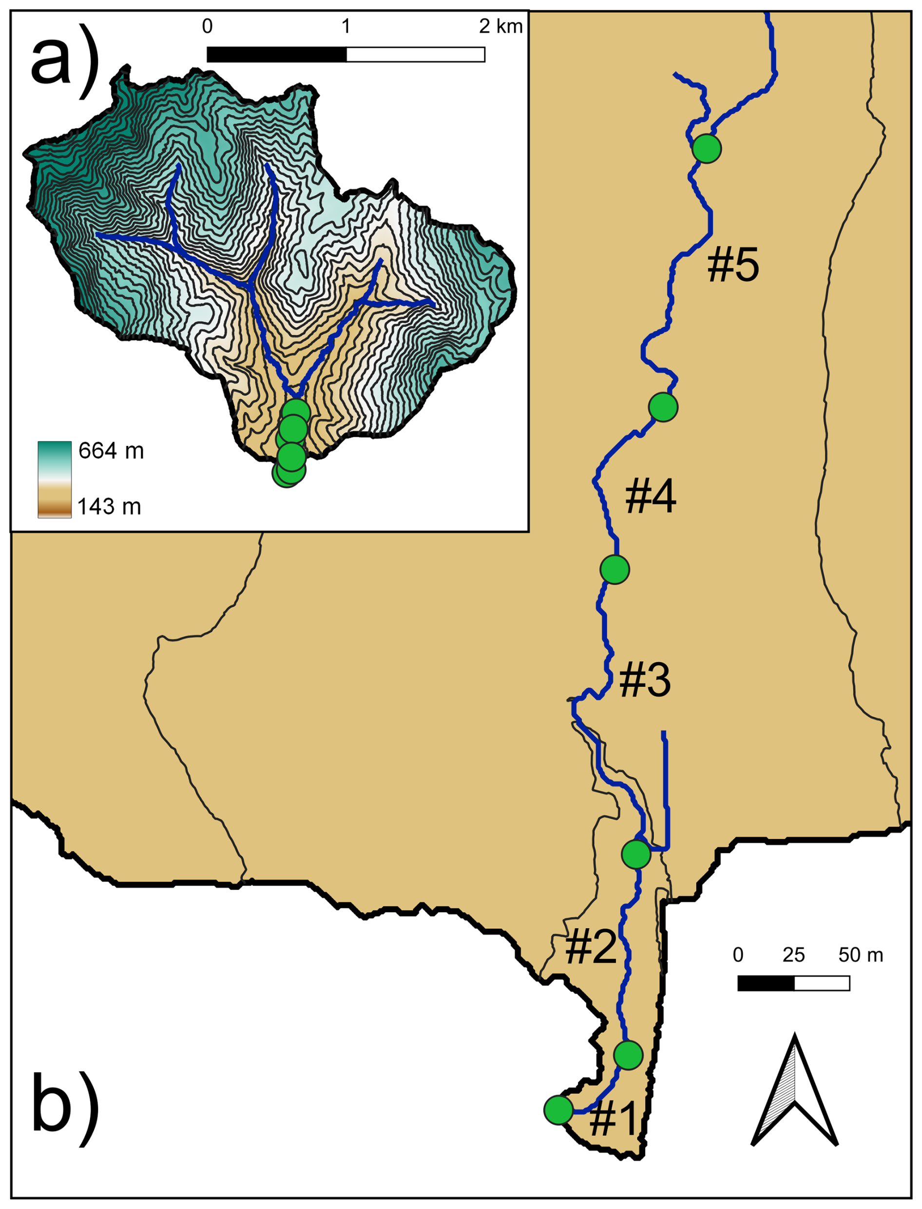
Figure 1 (a) Map of the Oak Creek catchment, with colors indicating elevation. Green markers denote tracer measurement locations. (b) Close-up view, where labels (#1–#5) represent reaches between these measurement locations.

Radon sampling sites were co-located with BTCs observations, collected one day before the slug tracer injections. We filled one-liter amber glass bottles with stream water in the thalweg and tightly closed the bottles beneath the water surface to prevent degassing during sampling. The water samples were analyzed using a large dome, large detector RAD7 device (Durridge Company, Inc.). We employed a closed air loop approach as outlined by Lee and Kim (2006). Each one-liter water sample underwent degassing with the integrated pump of the RAD7 to strip the dissolved radon into the air phase. Subsequently, radon in the air of the closed-loop was counted up to six times over 30 min with the integrated detector of the RAD7. The resulting average value of the repeated radon measurements was corrected for the time between sampling and measurement to account for radioactive decay. Radon measurements were then multiplied by an empirical correction factor to adjust for differences in degassing between one-liter samples and the reference volume of the RAD H₂O method (250 mL).

We determined the maximum radon activity that can be achieved based on the available radium-bearing minerals of Oak Creek (i.e., the radon activity reached at secular equilibrium). For this purpose, we selected two locations at Oak Creek and collected five sediment samples from each location. Subsequently, these sediment samples were merged into two bulk samples to reduce the potential for small-scale spatial heterogeneity in radon activity in the stream sediment, and to ensure representative sediment samples. We then conducted incubation experiments with stream sediment and radon-free water (after Corbett et al., 1997, 1998; Peel et al., 2022). After incubating the bulk sediment samples for at least 21 d inside gas-tight two-liter containers, we analyzed the water from these samples using the closed-loop approach with the RAD7, as described previously for the surface water samples. We assumed the same mineralogical composition of the aquifer and the streambed sediment. This means the radon activity at secular equilibrium represents both the radon activity of the groundwater and the highest achievable activity along subsurface flow paths.

2.2 Transient storage modelling

Solute transport parameters are commonly determined by calibrating TSMs against measured BTCs. TSMs describe the combined effect of flow velocity and dispersion on solute transport in a one-dimensional steady flow domain (Taylor, 1922, 1954), dilution (or enrichment) of solutes from lateral groundwater inflow, and additionally consider a first-order mass exchange of solutes between the surface and a finite-size, completely-mixed transient storage zone. The partial differential equations of the TSM are (Bencala and Walters, 1983):

$$\begin{array}{}\text{(1)}& \begin{array}{rl}{\displaystyle \frac{\partial C}{\partial t}}& =-{\displaystyle \frac{Q}{A}}{\displaystyle \frac{\partial C}{\partial x}}+{\displaystyle \frac{\mathrm{1}}{A}}{\displaystyle \frac{\partial }{\partial x}}\left(AD{\displaystyle \frac{\partial C}{\partial x}}\right)+{\displaystyle \frac{q_{\mathrm{I}}}{A}}(C_{\mathrm{I}}-C)\\ & +\propto \left(C_{\mathrm{TS}}-C\right),\\ & {\displaystyle \frac{\mathrm{d}{C}_{\mathrm{TS}}}{\mathrm{d}t}}=-\propto {\displaystyle \frac{A}{A_{\mathrm{TS}}}}\left(C_{\mathrm{TS}}-C\right)\end{array}\end{array}$$

where C is the observed tracer concentration above the background concentration [M L⁻³], t is time [T], Q the discharge in the stream channel [L³ T⁻¹], A the channel's cross-sectional area [L²], x the distance [L], D the longitudinal dispersion coefficient [L² T⁻¹], q_I the groundwater inflow into the stream channel [L³ L⁻¹ T⁻¹], α the transient storage exchange coefficient [T⁻¹], C_TS the solute concentration in the transient storage zone [M L⁻³], and A_TS the cross-sectional area of the transient storage zone [L²].

The model formulation above does not account for key processes affecting radon activity, as radon activity changes due to radioactive decay, degassing, and production in the transient storage zone (Cook, 2013; Frei and Gilfedder, 2015). Therefore, we implemented additional radon specific processes in the one-zone TSM as follows:

$$\begin{array}{}\text{(2)}& \begin{array}{rl}{\displaystyle \frac{\partial C}{\partial t}}& =-{\displaystyle \frac{Q}{A}}{\displaystyle \frac{\partial C}{\partial x}}+{\displaystyle \frac{\mathrm{1}}{A}}{\displaystyle \frac{\partial }{\partial x}}\left(AD{\displaystyle \frac{\partial C}{\partial x}}\right)+{\displaystyle \frac{q_{\mathrm{I}}}{A}}\left(C_{\mathrm{I}}-C\right)\\ & -\mathit{\lambda }C-{\displaystyle \frac{k}{d}}C+\mathit{\alpha }\left(C_{\mathrm{TS}}-C\right)\\ & {\displaystyle \frac{\mathrm{d}{C}_{\mathrm{TS}}}{\mathrm{d}t}}=-\propto {\displaystyle \frac{A}{A_{\mathrm{TS}}}}\left(C_{\mathrm{TS}}-C\right)-\mathit{\lambda }{C}_{\mathrm{TS}}+\mathit{\gamma }\end{array}\end{array}$$

where λ [T⁻¹] is the radioactive decay rate [(0.18 d⁻¹ for radon), k [L T⁻¹] the gas exchange velocity, d [L] the stream depth, and γ [M L⁻³ T⁻¹] the production of radon in the transient storage zone. In the absence of radon-specific processes (k=0, λ=0 and γ=0), Eq. (2) reduces to the TSM described in Eq. (1).

2.3 Numerical implementation of radon-specific processes in OTIS

The “One Dimensional Transport with Inflow and Storage” (OTIS) model (Runkel, 1998) is one of the most commonly used implementations of the TSM. OTIS uses a Crank-Nicolson numerical scheme to solve the TSM. We adapted the existing code of OTIS (written in FORTRAN 77) to simulate radon activity. Hereafter, we will refer to the implementation of the TSM that considers radon-specific processes as OTIS-R (R for radon; Bacher et al., 2025).

2.4 Model calibration

We used measured chloride concentrations and radon activity to calibrate the model parameters of the TSM. The calibration was done in a Monte Carlo approach to assess the model performance for different combinations of parameter values (after Kelleher et al., 2013; Ward et al., 2017). We refer to a single combination of calibrated parameter values as a “parameter set”. The same parameter sets were tested for both tracers to evaluate model performance for each tracer. The model performance was evaluated using the normalized root mean squared error (nRMSE). We performed this normalization to enable a relative comparison of both tracers. We conducted three different calibration approaches, each with 200 000 iterations. The model parameters were sampled using Latin Hypercube Sampling (LHS), a method that employs stratified sampling while retaining the simplicity and objectivity of fully random sampling (Helton and Davis, 2003). In all three calibration approaches, we calibrated D, α, and A_TS by sampling them from a defined parameter range (Table 1). We sampled parameter values of D, α, and A_TS uniformly from a log10 transformed space to ensure approximately equal representation for each order of magnitude within the parameter space (Kelleher et al., 2013; Ward et al., 2017). We extracted the 1 % and 10 % with the lowest values for the nRMSE of the parameter sets and considered them as behavioral parameter sets (Beven and Binley, 1992). We selected these behavioral thresholds to ensure consistency with previous solute transport studies (e.g., Bonanno et al., 2022; Kelleher et al., 2019; Wagener et al., 2002; Ward et al., 2013, 2017; Wlostowski et al., 2013). Since we tested the same combinations of parameter values in the TSM for both tracers, the intersection of the behavioral parameter sets from both tracers reflects the parameter sets obtained when the model is calibrated with both tracers together. This indicates that when the behavioral parameter sets for both tracers are identical, the choice of tracer does not affect estimates of solute transport. We refer to this intersecting set as the “joint calibration”. In contrast, other parameter sets were included in the behavioral set for only one tracer but not the other. These sets represent parameterizations that result in acceptable model performance for a single tracer, but are not robust in simulating both tracers simultaneously. We refer to these as the “individual calibration”. The behavioral parameter sets were used for all subsequent analysis and calculations.

Table 1 Calibration parameters used in OTIS-R. Parameter ranges are shown for those that were calibrated.

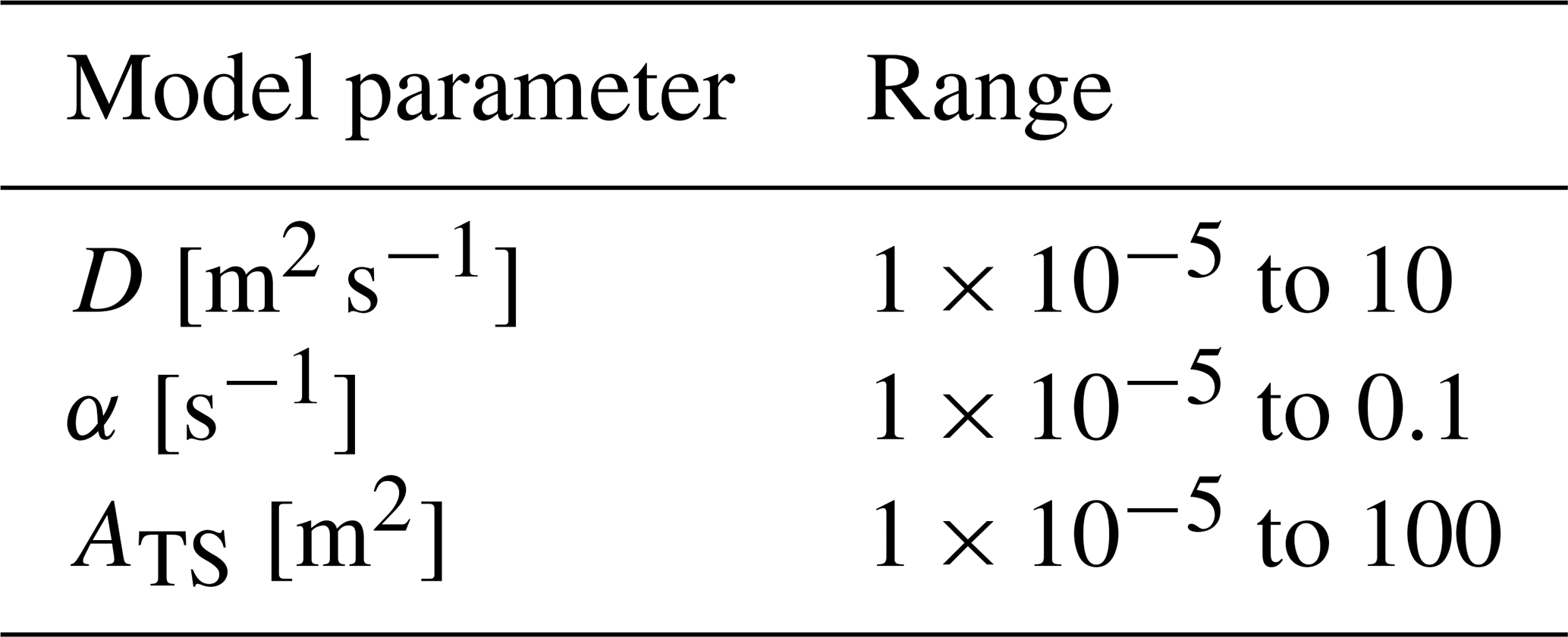
Model parameters other than those calibrated – including the stream velocity (v), the cross-sectional area (A), the production term of radon in the storage zone (γ), and the gas exchange velocity (k) – were calculated before calibration. This reduces potential issues of equifinality with TSMs (Knapp and Kelleher, 2020). We calculated v by dividing the stream length by the arrival time of the concentration peak of the downstream BTC, and calculated A from v and Q after the calibration approach. This choice was motivated by findings from Bonanno et al. (2022), who showed that A_TS and α are often not identifiable when v is calibrated instead of calculating v by dividing the stream length by the arrival time of the concentration peak of the downstream BTC. We calculated the radon production term γ as the product of the decay constant (0.18 d⁻¹) and the measured equilibrium radon activity (Gilfedder et al., 2019). This approach assumes that radon production occurs only in the subsurface transient storage zone of the stream. However, radon may also increase when stream water interacts directly with the streambed surface. For the gas exchange velocity, we relied on gas tracer experiments previously conducted at the same stream section as our study at Oak Creek (Cargill et al., 2021). We scaled the gas exchange coefficients for SF₆ reported by Cargill et al. (2021) to radon (Jähne et al., 1987; Raymond et al., 2012). We tested two different gas exchange velocities for each run of our three calibration approaches to quantify the uncertainty of degassing in calibration of the TSM. The gas tracer experiments by Cargill et al. (2021) were conducted at three different discharge conditions (0.05, 0.1, 1.07 m³ s⁻¹). We used values from the experiments conducted during the lowest and highest discharges for parameterization. This resulted in one model setup with a low gas exchange value and another with a high gas exchange value. Hereafter, we will refer to these different values used for parameterization as k_low (k₆₀₀=206 d⁻¹) and k_high (k₆₀₀=290 d⁻¹).

2.5 Evaluating parameter sensitivity, certainty, and interactions

After model calibration, we evaluated the parameter identifiability of the behavioral parameters through sensitivity, certainty, and interactions analysis. We refer to a parameter set as “identifiable” when the values of the model parameters are sensitive, certain, and do not have any parameter interactions. The parameter identifiability analyses include the visual inspection of (I) nRMSE vs. parameter plots (Wagener et al., 2003), (II) cumulative parameter distribution plots (Kelleher et al., 2019), (III) posterior distribution plots (Wagener et al., 2002; Ward et al., 2017), (IV) scatter plots of the behavioral parameters, and V) calculation of the Shannon entropy for the posterior distribution of model parameters as metric for certainty (sensu Rodriguez et al., 2021, Sect. 2.6). In the nRMSE vs. parameter plots, parameters needed to exhibit a distinct peak of performance in nRMSE to be categorized as sensitive. Furthermore, the cumulative distribution functions (CDFs) of the top 1 % or 10 % of results (behavioral parameters) had to visibly deviate from the 1:1 line (representing a uniform distribution) to be categorized as sensitive. The probability density functions (posterior distributions) had to be peaked and narrow to categorize parameters as certain.

The posterior distribution of parameters is represented by the histogram of behavioral parameter sets and their performance (nRMSE). This histogram was created by dividing the parameter values into 15 equally sized bins, where the bar height illustrates the likelihood of a parameter falling within a specific bin. Certain parameters exhibit higher variation in likelihood across different parameter values. In the scatter plots, narrow and constrained values of two model parameters indicate identifiable parameters. Parameter interactions are visible through changes in the value of one parameter relative to changes in another within the parameter space. These interactions are visually depicted as a curve in the parameter space, suggesting that variations in parameter 1 result in corresponding variations in parameter 2.

For a quantitative measure of the parameter sensitivity that underpins the visual inspections, we applied the two-sample Kolmogorov–Smirnov (K–S) test that calculates the maximum distance K and the corresponding p-value between two cumulative distribution functions:

$$\begin{array}{}\text{(3)}& \left[K,p\right]=max|F\left(P_{\text{behavioral}}\right)-F\left(P_{\text{non-behavioral}}\right)|\end{array}$$

where F(P_behavioral) and F(P_{non-behavioral}) are the cumulative distribution functions of a parameter P for the behavioral and non-behavioral parameter sets, respectively. The K–S test thus expresses the degree of sensitivity for a parameter. We grouped parameter sensitivity into four different categories following the approach of Ouyang et al. (2014): highly sensitive (K>0.2; p-value ≤ 0.05), moderately sensitive $\mathrm{0.1}\le K\le \mathrm{0.2}$; p-value ≤ 0.05), poorly sensitive (K<0.1; p-value ≤ 0.05) and non-sensitive (p-value > 0.05). Moreover, we calculated the non-parametric Spearman rank correlation coefficient (p_spearman) using a significance threshold of 0.05 to quantitatively assess the non-linear interactions between different model parameters observed in the scatter plots.

2.6 Evaluating information content of model parameters

We evaluated parameter certainty using the information content, calculated as the Shannon entropy of the posterior distributions of model parameters (Cover and Thomas, 2006; Loritz et al., 2018). Rodriguez et al. (2021) applied this approach in a catchment-scale study. The posterior distribution is the probability density function of the behavioral parameters sets. The Shannon entropy reads:

$$\begin{array}{}\text{(4)}& H\left(X|T\right)=-\sum _{k=\mathrm{1}}^{n_{\mathrm{I}}}f\left(I_k\right){\log }_{\mathrm{2}}f\left(I_k\right)\end{array}$$

where H describes the Shannon entropy and X the parameter of interest. T is the tracer, for which behavioral parameter sets were extracted. The tracer could either be radon, chloride or a combination of both ($H\left(X\right|(\mathrm{radon}\bigcap \mathrm{chloride}))$). We binned the parameter values into 15 bins of equal size, similar to visual inspection of the posterior distribution of the parameter certainty. The rationale for choosing 15 bins was that the resulting histograms visually revealed the underlying structure of the parameter values without introducing uneven features, such as spiky histograms. The height of each bin describes the likelihood of the parameter being located in this specific bin. n_I [–] signifies the number of intervals (bins), and f(I_k) [–] describes the probability of the parameter X falling within the interval I_k. f(I_k) describes the probability of the parameter X to take a value in an interval I_kfor the posterior distribution (either radon, chloride, or a combination of both) or the prior distribution (none of those). Smaller values of H show that the posterior distribution is not flat and that it is more certain than a uniform prior distribution.

Furthermore, we evaluated the information gain from the prior to the posterior distribution of model parameters when the TSM was calibrated with radon and chloride separately, as well as for both tracers together. In this context, the prior distribution describes the uniform distribution of all parameters prior to parameter calibration. The minimum and maximum values for this distribution are defined through the parameter range from which these parameters were sampled (Table 1). The information gain quantifies how much information the tracers add to the model parameters when calibration of the model was conducted with these tracers separately and with both tracers together. We evaluated the information gain from prior to posterior distributions for each model parameter using the Kullback-Leibler divergence D_KL (Rodriguez et al., 2021):

$$\begin{array}{}\text{(5)}& D_{\mathrm{KL}}\left(X|T,X\right)=\sum _{k=\mathrm{1}}^{n_{\mathrm{I}}}f\left(I_k\right){\log }_{\mathrm{2}}{\displaystyle \frac{f\left(I_k\right)}{g\left(I_k\right)}}\end{array}$$

where g(I_k) [–] is the probability of the parameter X to fall in the interval I_k in the prior distribution. Higher values of D_KL (in bits) show a higher information gain from prior to posterior parameter distribution during calibrating the model (Rodriguez et al., 2021). Summing values of the Kullback-Leibler divergence for all TSM parameters yields the total information on solute transport from that tracer.

2.7 Accounting for groundwater inflow in TSM calibration

Radon activity in streams varies with the amount of inflowing groundwater, as radon activity differs significantly between groundwater and surface water (Cook, 2013). Small changes in the amount of inflowing groundwater may lead to differences in model performance. To account for this, we either calibrated or calculated groundwater inflow within three different calibration approaches, in addition to calibrating D, α, and A_TS. These approaches to handling groundwater inflow were selected to assess how varying values of groundwater inflows affect model performance. For the first calibration approach (Q_fix), we calculated the groundwater inflow by dividing the difference of discharge between the upstream and downstream BTCs by the reach length. In the second calibration approach (Q_LHS), discharge was calibrated as model parameter, like D, α, and A_TS, before calculating groundwater inflow. For each reach, discharge was sampled from a normal distribution, because Schmadel et al. (2010) reported that discharge measurement errors follow a normal distribution. We used the calculated discharge as the mean of the normal distribution and assumed that its standard deviation represents the uncertainty of dilution gauging. In the third calibration approach (Q_out), we directly calibrated groundwater inflow, whereas discharge was not calibrated. The direct calibration of groundwater inflow allows us to calculate gross water fluxes along reaches. This is because OTIS, and by extension OTIS-R, accounts for water mass balance under steady state by parameterizing groundwater inflow using the following equation:

$$\begin{array}{}\text{(6)}& {\displaystyle \frac{\partial Q}{\partial x}}=I-O\end{array}$$

where I [L² T⁻¹] is the gross water inflow and O [L² T⁻¹] the gross water outflow from the stream into the groundwater. The discretized form of this equation, with ΔQ describing the difference of discharge between the upstream and downstream BTCs and Δx the reach length, can be expressed in terms of q_out [L³ T⁻¹ L⁻¹] rather than O. In the first and second calibration approaches, gross water outflow was assumed to be zero. These gross water fluxes are commonly derived from calculating the mass loss of BTCs relative to the injected tracer mass (i.e., “channel water balance”; Payn et al., 2009). For all three calibration approaches, the measured equilibrium radon activity was used as the activity of the groundwater inflow.

Additionally, radon activity in streams depends on the location of the groundwater flow (Cook, 2013). Assuming groundwater inflow as either discrete or linear in the TSM might therefore lead to different simulated radon activity and, in turn, to different calibrated parameter values to achieve a good fit between simulated and measured radon activity. To test this, we calibrated the TSM with radon activity for the downstream-most reach in three different model setups. In each setup, we assumed different locations of groundwater inflow along the selected reach (upstream-most point, mid-point, and downstream-most point in the study reach). The sub-reach with the groundwater inflow attributed to a 1 m long subdivision and at a magnitude equal to the total net increase in stream flow along the study reach (i.e., all groundwater inflow in a single location, representing a focused discharge of groundwater into the stream, like that attributable to a geologic discontinuity or fracture). For each of the three model setups, we ran the model 200 000 times and calibrated the model parameters (D, α, A_TS, discharge) following the same procedures as the prior model fitting. We then compared calibrated model parameters among the different model setups and applied identifiability analysis to the behavioral parameter sets (1 % and 10 %). Subsequently, we applied the Levene test for equality of variance to compare the distributions of the model parameters from the different model setups (upstream, middle, downstream), using a p-value of 0.05 for determining statistical significance. Although we expect groundwater inflow to primarily affect radon activity in streams, we also calibrated TSM parameters in three model setups that varied in groundwater inflow locations using chloride concentrations. This was motivated by the assumption that chloride-free groundwater, as commonly assumed in TSMs, dilutes chloride concentrations in streams.

3 Results

3.1 Tracer concentration in Oak Creek

BTCs (Fig. S1) showed a distinct peak concentration at both the upstream and the downstream locations of the study reaches, thereby meeting a key requirement for the calibration of the TSM. Radon activity in groundwater was 23 times higher than in surface water, providing the necessary contrast for quantifying groundwater inflows into the stream. Stream radon activity ranged from 285 (±22) Bq m⁻³ to 337 (±26) Bq m⁻³ with the highest activity was observed at reach #2 (Table S1).

3.2 Information content and information gain for model parameters

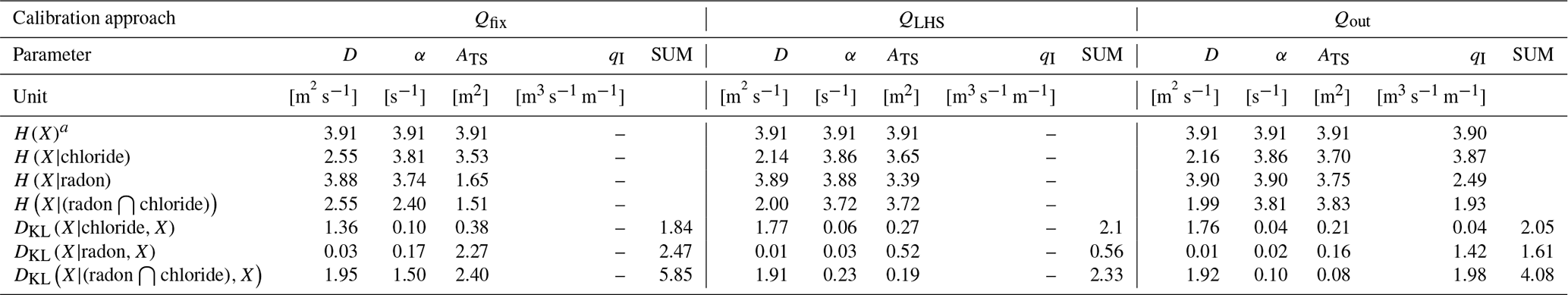
TSM calibration with both tracers resulted in higher values of the Kullback-Leibler divergence and thus more information on model parameters compared to calibration with chloride or radon alone ($D_{\mathrm{KL}}\left(X\left|\right(\mathrm{radon}\bigcap \mathrm{chloride}),X\right)\mathit{>}{D}_{\mathrm{KL}}\left(X|\mathrm{chloride},X\right)$ and $D_{\mathrm{KL}}\left(X\left|\right(\mathrm{radon}\bigcap \mathrm{chloride}),X\right)\mathit{>}{D}_{\mathrm{KL}}\left(X|\mathrm{radon},X\right))$ (Table 2). When calibrating the TSM with each tracer alone, chloride provided more information on model parameters than radon ($D_{\mathrm{KL}}\left(X|\mathrm{chloride},X\right)\mathit{>}{D}_{\mathrm{KL}}\left(X|\mathrm{radon},X\right))$. The only exception occurred in the calibration approach with fixed groundwater inflow (Q_fix). Values of the Kullback-Leibler divergence of individual parameters varied depending on the tracer used for calibration. In general, chloride provided more information on D but little information on groundwater inflow q_I, whereas radon provided more information on groundwater inflow q_I but less on D.

Calibrating the TSM with both tracers increased certainty in model parameters compared to using chloride and radon alone. This is evident in values of the Shannon entropy of the model parameters, which show that the posterior distributions became narrower ($H\left(X\left|\right(\mathrm{radon}\bigcap \mathrm{chloride})\right)\mathit{<}H\left(X\right)$; (Table 2)). Similarly, TSM calibration with each tracer alone increased certainty in the model parameters ($H\left(X|\mathrm{radon}\right)<H\left(X\right)$ and $D_{\mathrm{KL}}\left(X\left|\right(\mathrm{radon}),X\right)\mathit{>}\mathrm{0}$ and ($H\left(X|\mathrm{chloride}\right)<H\left(X\right)$ and $D_{\mathrm{KL}}\left(X\left|\right(\mathrm{chloride}),X\right)\mathit{>}\mathrm{0}$).

Table 2 Shannon entropy H and Kullback-Leibler divergence D_KL for the prior and posterior distributions of model parameters (D, A_TS, α and the groundwater inflow q_I) resulting from joint ($H\left(X\right|\mathrm{radon}\bigcap \mathrm{chloride})$; $D_{\mathrm{KL}}\left(X\right|(\mathrm{radon}\bigcap \mathrm{chloride}),X)$) and individual (H(X|chloride); H(X|radon); D_KL(X|chloride); D_KL(X|radon))) calibration of the TSM with chloride and radon. Results from all three calibration approaches are shown here, which differ in how groundwater inflow was calibrated (Q_fix, Q_LHS, and Q_out). For simplicity, only the results of the top 10 % behavioural parameter sets from the low-degassing model setup (k_low) with radon are shown here for reach #1. Results for reaches #2–#5 can be found in the supporting information (Table S2).

3.3 Parameter sensitivity and certainty

Parameter sensitivity and certainty depended on the tracer used for calibration. When the TSM was calibrated with chloride, D showed high sensitivity, whereas groundwater inflow was largely insensitive (Table 3). Calibrating the TSM with radon resulted in no sensitivity to D but high sensitivity to groundwater inflow. The sensitivity and certainty of A_TS and α in simulations depended both on the tracer used for calibration and the approach used to calibrate groundwater inflow (Figs. 2, 3, 4, Tables 3, S3). Calibration with chloride consistently resulted in high parameter certainty and moderate to high sensitivity for A_TS and α. In contrast, calibration with radon yielded moderate to high sensitivity of A_TS and α when groundwater inflow was fixed (Q_fix). A_TS and α became insensitive when groundwater inflow was included as a direct calibration parameter (Q_out) or calculated from calibrated discharge (Q_LHS). A comparison of model performance showed that the nRMSE values of behavioral parameter sets were lower when calibrating with radon than with chloride (Fig. 2).

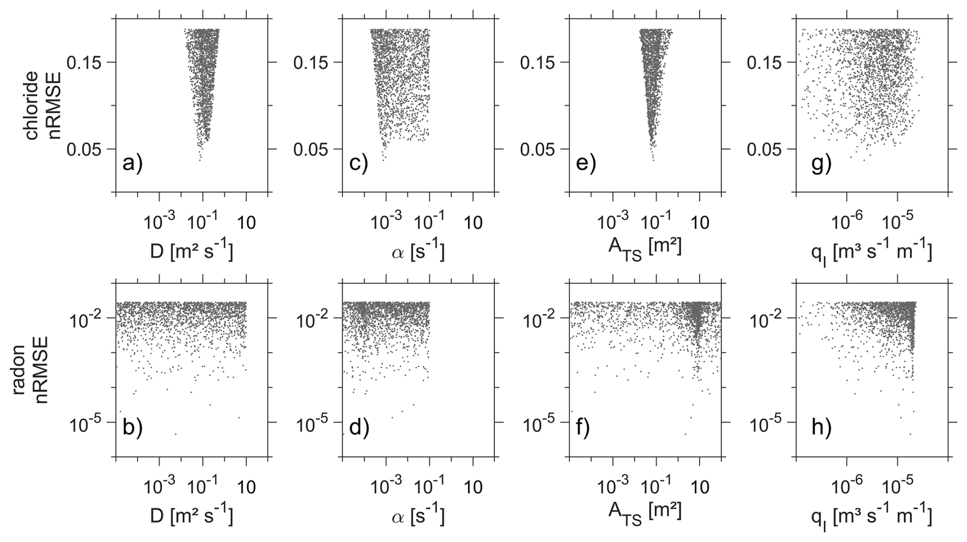
Figure 2 Parameter values (D, α, A_TS, and the groundwater inflow (q_I)) plotted against the corresponding normalized root mean square error (nRMSE) values. The figure shows the best 1 % of model runs from calibrating the TSM with chloride (top row) and radon (bottom row) using the calibration approach in which groundwater inflow q_I was calculated from calibrated discharge (Q_LHS). The model runs shown are from reach #1. For radon, we present the k_low model setup only.

Table 3 Overview of the sensitivity based on the K–S test for all model parameters (D, α, A_TS, and the groundwater inflow (q_I)) from the individual calibration of the TSM with chloride and radon. The terms “high”, “moderate”, “poor”, and “non-sensitive” refer to the classification of parameter sensitivity based on the K-value and p-value (see Sect. 2.6), following the methodology of Ouyang et al. (2014). Results from all three calibration approaches are shown here, which differ in how groundwater inflow was calibrated (Q_fix, Q_LHS, and Q_out). Results are presented for all reaches, but only for the 1 % behavioral parameters. For simplicity, we show the k_low model setup for calibrating the TSM with radon only.

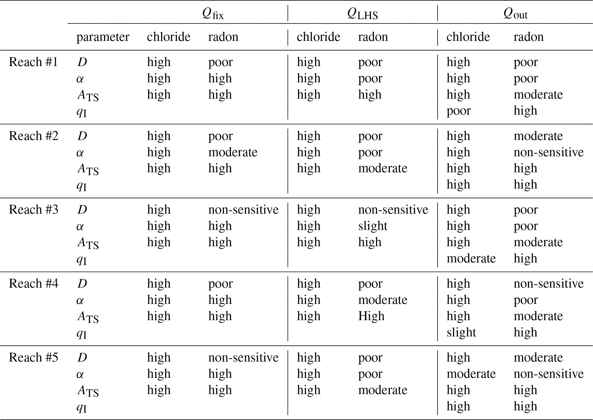
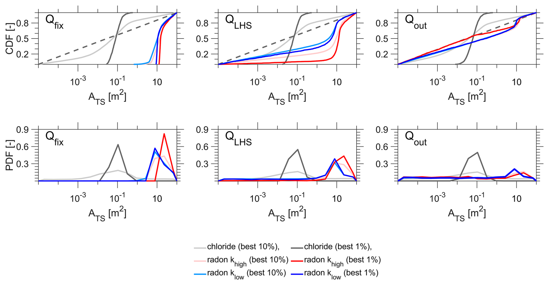
Figure 3 Cumulative distribution plots (upper row) and posterior distribution plots (lower row). Each plot shows A_TS results based on the best 1 % and best 10 % parameter sets from the individual calibration. We present results from the calibration approach where groundwater inflow was fixed (Q_fix), calculated from calibrated discharge (Q_LHS), and directly calibrated (Q_out). Non-behavioral A_TS parameters in the top row are shown with a grey dashed line. For simplicity, we show the results from reach #1 only.

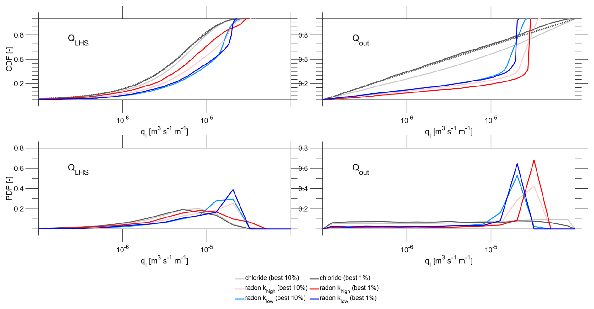
Figure 4 Cumulative distribution plots (upper row) and posterior distribution plots (lower row). Each plot shows groundwater inflow (q_I) results based on the best 1 % and best 10 % parameter sets from the individual calibration. We present results from the calibration approach where groundwater inflow was fixed (Q_fix), calculated from calibrated discharge (Q_LHS), and directly calibrated (Q_out). Non-behavioral q_I parameters in the top row are shown with a grey dashed line. For simplicity, the results from reach #1 are shown only.

3.4 Parameter interactions

We found no parameter interactions when the TSM was calibrated with chloride, with only a few exceptions (Fig. 5, Table S4). Calibration with chloride resulted in a narrower range between the minimum and maximum values of the behavioral parameters, thereby better constraining parameter values. In contrast, when the TSM was calibrated with radon, parameters were tightly constrained only when others in the same set were less constrained (Fig. 5). For example, groundwater inflow was tightly constrained at higher values within the behavioral parameter range, but A_TS values for these groundwater inflow values remained unconstrained. Conversely, when A_TS values were tightly constrained at higher values, groundwater inflow values associated with them were unconstrained.

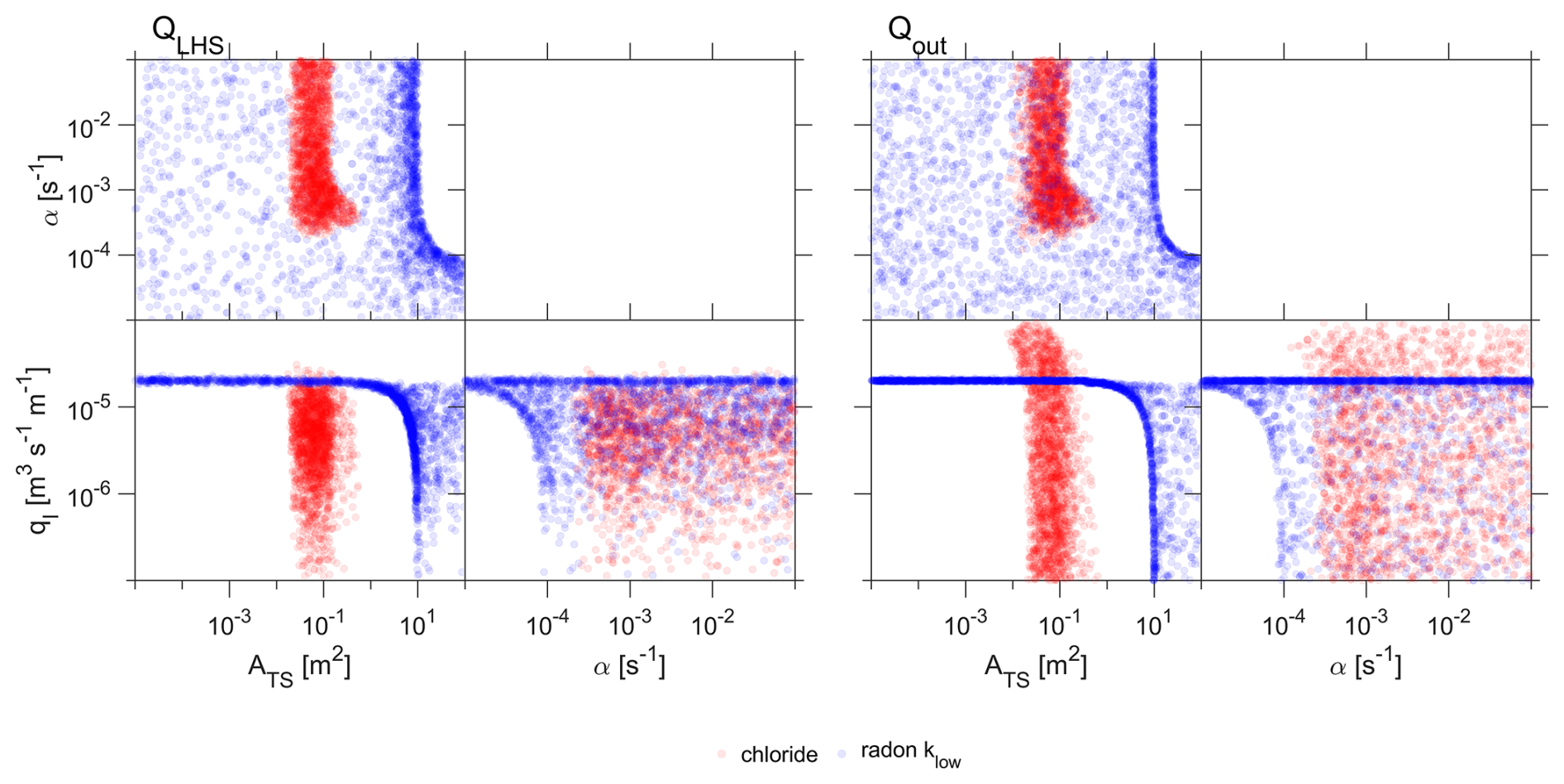
Figure 5 Scatter plots of the best 1 % model parameters (A_TS, α and q_I) from calibrating the TSM with radon (blue) and chloride (red) alone. Calibration with chloride resulted in constrained parameter values. When the TSM was calibrated with radon, parameter values were tightly constrained only when others in the same set were less constrained. We show the calibration approach where the groundwater inflow was calculated from calibrated discharge (Q_LHS) and the calibration approach where the groundwater inflow was directly calibrated (Q_out). For simplicity, only the results from calibrating the TSM with radon in the k_low model setup are shown. The parameter D is not included, as it was neither certain nor sensitive in calibrating the TSM with radon.

3.5 The effect of different locations of groundwater inflow on parameter interactions

We found significantly different distributions of the behavioral parameters dependent on the different locations of groundwater inflow (upstream-most point, mid-point, downstream-most point model setups) independently of which tracer was used for calibration (Figs. 6, 7). Calibrating the TSM with chloride resulted in constrained parameters when the inflow was located at the upstream-most point or mid-point (Fig. 7). In contrast, parameter interactions became evident when inflow was at the downstream-most point. When the TSM was calibrated with radon and groundwater inflow was set at the upstream-most point, A_TS was tightly constrained at higher values within the behavioral parameter range. However, the groundwater inflow values remained unconstrained for these higher A_TS values. In contrast, parameter values were less constrained when inflow was set at the downstream-most point.

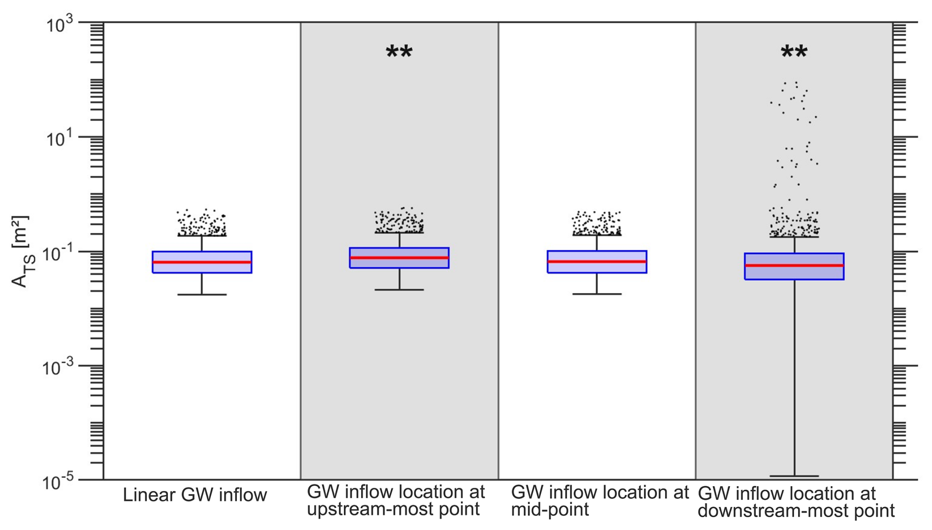
Figure 6 Distributions of behavioral A_TS values from model setups with varying groundwater inflow locations, each calibrated with chloride only. The model setup labelled “linear groundwater (GW) inflow” refers to the calibration approach where the groundwater inflow was calculated from the calibrated discharge (Q_LHS). The red line is the median of the distributions, while black dots highlight outliers. Asterisks and the grey areas show a significant difference between the variance of the parameter distributions compared to the setup with linear groundwater inflow. Results are shown for the best 1 % behavioral model parameters and reach #1 only.

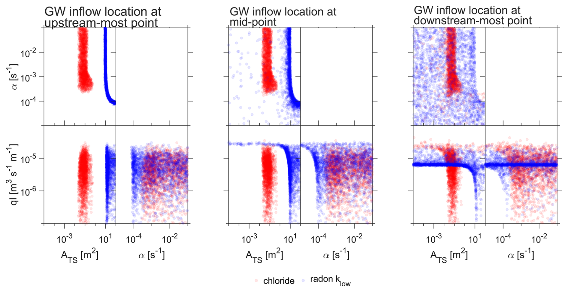
Figure 7 Scatter plots of the best 1 % behavioral model parameters (A_TS, α and the groundwater inflow q_I) from calibrating the TSM with radon and chloride alone. Three different model setups are presented that differ in the location of the groundwater inflow along the reach (upstream-most point, mid-point, downstream-most point model setups). For simplicity, results from calibrating the TSM with radon in the k_low model setup are shown only.

3.6 Gross water fluxes from the TSM calibrated with radon and chloride

Discharge gradually increased in the downstream direction and ranged from 9.5 to 12 L s⁻¹ across all reaches (Fig. 8a). However, not all reaches exhibited this increase; specifically, discharge decreased in reaches #1 and #4. Gross loss and gain revealed spatial variability across reaches. Reaches #1 and #4 were characterized by higher gross losses compared to remaining reaches (Fig. 8b). Notably, gross water flux could only be derived from calibrating the TSM with radon and not with chloride.

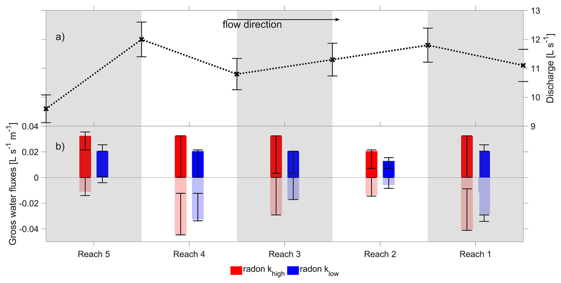
Figure 8 (a) Discharge values upstream and downstream of each reach [L s⁻¹] with 95 % confidence intervals. Discharge was calculated from BTCs using dilution gauging. (b) Gross water fluxes [L s⁻¹ m⁻¹] for each reach, derived from calibrating the TSM with radon measurements (Q_out). Both degassing model setups are shown (blue and red) and transparent bars highlight negative water fluxes. Bar heights correspond to the mode of the posterior distribution for the calibrated q_I and calculated q_out values. Error bars show the 95 % confidence interval of the posterior distribution.

4 Discussion

4.1 Calibrating TSMs with multiple tracers better constrains model parameters

Calibrating the TSM with chloride provides more information on solute transport than calibrating with radon because chloride is particularly informative on D (Table 2). Previous studies have shown that D mainly affects the rising limb of BTCs (e.g., Kelleher et al., 2013; Wlostowski et al., 2013). This highlights that a tracer with a distinct rising concentration limb, such as chloride, is necessary to identify D. Radon, by contrast, provides more information on groundwater inflow and A_TS than chloride (Table 2) due to its higher activity in groundwater compared to surface water. Because chloride concentrations are lower in groundwater compared to surface water, groundwater inflow simply dilutes chloride concentrations in the stream without adding additional information on inflow. In summary, the most information on solute transport is obtained by using both tracers jointly because each tracer contributions uniquely. Joint calibration with radon and chloride improves certainty in solute transport estimates compared to calibrating with either tracer alone. We therefore recommend calibrating TSMs with multiple tracers to improve estimates of solute transport in future studies.

This recommendation aligns with recent calls for joint calibration of hydrological models with multiple tracers. For example, Neilson et al. (2010b) demonstrated that calibrating a TSM with both temperature and slug tracer data provides more insights into solute transport and exchange compared to calibrating the TSM with temperature alone. At the catchment scale, Rodriguez et al. (2021) demonstrated that jointly calibrating a storage selection function with deuterium and tritium reduced uncertainty in model parameters compared to calibrating with either tracer alone. Notably, the authors used a different quality criterion for behavioral parameter selection than we did. Rodriguez et al. (2021) used distinct threshold values for each tracer to obtain a comparable number of behavioral parameter sets due to differences in sampling frequency, and thus dataset length, between deuterium and tritium. In contrast, we selected the best 1 % and 10 % of parameter sets as behavioral to remain consistent with previous solute transport studies (e.g., Kelleher et al., 2019; Wagener et al., 2002; Ward et al., 2013, 2017; Wlostowski et al., 2013). This selection resulted in a lower nRMSE for radon compared to chloride (Fig. 2), thus carrying more weight in the joint calibration. Therefore, the conclusion that joint calibration of the TSM with radon and chloride yields more information than calibration with either tracer alone is partly influenced by the quality criterion for parameter sets and, ultimately, by subjective modeling decisions – a well-known challenge in hydrology (e.g., Beven and Binley, 1992).

4.2 The role of groundwater inflow for parameter identifiability

The sensitivity of radon to the amount and location of groundwater inflow makes it difficult to obtain narrow, well-constrained estimates for groundwater inflow, A_TS, and α, when calibrating TSMs with radon alone. The sensitivity to the amount of groundwater inflow is evident in the calibration approach where groundwater inflow was calculated from calibrated discharge (Q_LHS; Fig. 5). Discharge was sampled within the uncertainty range of measurements (95 % confidence interval from dilution gauging). Even within this range, varying groundwater inflow values led to wide, unconstrained values of A_TS and α. This suggests that constraining groundwater inflow, A_TS, or α with radon calibration alone will remain challenging unless at least one of these parameters is independently constrained. Deriving narrow, well-constrained TSM parameters is also restricted due to the sensitivity of radon to the location of groundwater inflow. This is shown by different parameter interactions across model setups that vary in the location of groundwater inflow (Fig. 7). For example, when groundwater inflow occurs at the downstream-most point in the study reach, radon activity increases there, where measured radon activity is used for calibration. A shorter distance between inflow and this point means less time for radon degassing. With less degassing time, only smaller and better constrained groundwater inflow values can close the radon mass balance and achieve a good fit between simulated and measured radon activity. However, these constrained groundwater inflow values lead to less-constrained A_TS and α estimates, since different combinations of these parameters can still close the radon mass balance. Therefore, spatial variability in groundwater inflow hampers precise constraints A_TS and α when using radon alone for model calibration.

Spatially heterogeneous groundwater inflows have been documented across various streams and attributed to transitions in valley structure (Mallard et al., 2014; Cartwright and Gilfedder, 2015; Payn et al., 2009; Pittroff et al., 2017; Somers et al., 2016), geological fractures (Genereux et al., 1993; Glaser et al., 2020), or subsurface textural heterogeneities (Fleckenstein et al., 2006). Groundwater inflows at discrete stream locations are common (Sophocleous, 2002). However, their effect on the identifiability of TSM parameters has not been explored. Previous research has instead highlighted the critical role of degassing when simulating radon activity (e.g., Atkinson et al., 2015; Gilfedder et al., 2019). For example, Schubert et al. (2020) incorporated degassing tests alongside radon measurements to quantify groundwater inflow using a numerical mass balance approach with transient storage parameters. They found that calibrated groundwater inflows exceeded the net increase in discharge, attributing this outcome to spatial variability in degassing rates. In our study, the two degassing parameterizations did not affect model performance (e.g., Figs. 3 and 4). Instead, differences in groundwater inflow locations along the reach resulted in different model parameters in behavioral parameter sets. Although our study site differs from Schubert et al.'s (2020), both models assume linear groundwater inflow along the reach. Therefore, the overestimation of calibrated groundwater inflows by Schubert et al. (2020) may also result from spatial variability in groundwater inflows along their study reach, which causes radon increases that require higher calibrated groundwater inflow values. Similarly, Cook et al. (2006) reported an overestimation of groundwater inflow to the Cockburn River, Australia, by almost 70 % compared to actual flow measurements. The authors concluded that including exchange with subsurface transient storage zones is essential when simulating radon activity. An underlying assumption of their model approach was linear inflow along the reach, similar to Schubert et al. (2020). In light of our findings, we suggest that the overestimation found by Cook et al. (2006) may instead be due to spatial variability in groundwater inflows, rather than solely the omission of exchange with subsurface transient storage zones in their radon mass balance. Therefore, our findings emphasize that the spatial variability of groundwater inflow location should be explicitly accounted for in future radon-based studies. This consideration may challenge the common perception that radon mass balances can be fully closed solely by including exchange with subsurface transient storage zones.

Notably, our results show that spatially heterogeneous groundwater inflows also affect the identifiability of α and A_TS when calibrating the TSM with chloride concentrations (Fig. 6). Previous studies reported uncertainty in α estimates from the behavioral parameters when calibrating TSMs with chloride concentrations (Kelleher et al., 2013; Wagener et al., 2002; Wlostowski et al., 2013). These studies linked the uncertainty to differences in stream-specific characteristics. Our findings provide a more detailed explanation: the spatial variability in groundwater inflow along streams. We thus suggest further research to understand how groundwater inflow affects chloride concentrations and, consequently, the identifiability of parameters in TSM calibration. Future studies on solute transport with chloride should first identify groundwater inflow locations before selecting a reach for slug tracer injections. This could be done by incorporating spatially resolved piezometers and hydraulic head measurements along streams, as implemented in the study design of Harvey and Bencala (1993) and Bonanno et al. (2023). Alternatively, temperature surveys (distributed temperature sensing; “DTS”), which provide high spatial and temporal resolution data on longitudinal groundwater inflows (Krause and Blume, 2012), could be used.

4.3 Radon is biased toward large spatial-scale subsurface flow paths

Spatially variable gross water gains exceeding net discharge from TSM calibration with radon suggest that the water balance of Oak Creek is affected by stream–subsurface water exchange that is occurring at multiple spatial scales. Previous studies have shown that large spatial-scale subsurface flow paths, that are subsurface flow paths originating from further upstream of the stream reach, play a critical role in explaining water mass balances in streams (e.g., Payn et al., 2009; Stanford and Ward, 1993; Ward et al., 2023). Unlike chloride, radon uniquely labels these flow paths (Fig. 9, arrow C), which would be undetectable if chloride were used. This unique labeling underpins the superior sensitivity of radon in revealing subsurface flow paths and highlights its novel contribution to understanding the role of these flow paths in stream water balances. Conceptually, this labeling capacity of radon is reflected in measured steady state activity at both the upstream and downstream ends of the reach before the slug tracer experiment began. Steady state activity indicates that the measured radon activity includes subsurface water parcels pre-labelled with radon prior to the experiment. Thus, large spatial-scale subsurface flow paths from further upstream also contribute to measured radon activity at the downstream end of the reach (Fig. 9, arrow C), along with groundwater inflow and temporally shorter flow paths (Fig. 9, arrows A, B, and E; McCallum et al., 2012). In contrast, chloride is injected as a distinct input signal (Dirac injection) at the upstream end of the reach and thus only reveals flow paths between locations of injection and measurement (Fig. 9, arrows A and B). This inherent bias of chloride injections toward labeling timescales within the WoD complements the bias of radon toward large spatial-scale subsurface flow paths, underscoring the value of using both tracers together. However, despite these novel insights on large spatial-scale flow paths from calibrating TSM with radon, such paths are not explicitly represented in the TSM. Instead, they are indirectly accounted for through the calibration of groundwater inflow. This indirect consideration may lead to an overestimation of groundwater inflow values during calibration. Such overestimation reduces certainty in the A_TS and α parameters and causes interactions among groundwater inflow, A_TS, and α. Although radon's sensitivity to large spatial-scale subsurface flow paths provides valuable insights, it therefore also introduces bias in constraining transient storage parameters in TSMs.

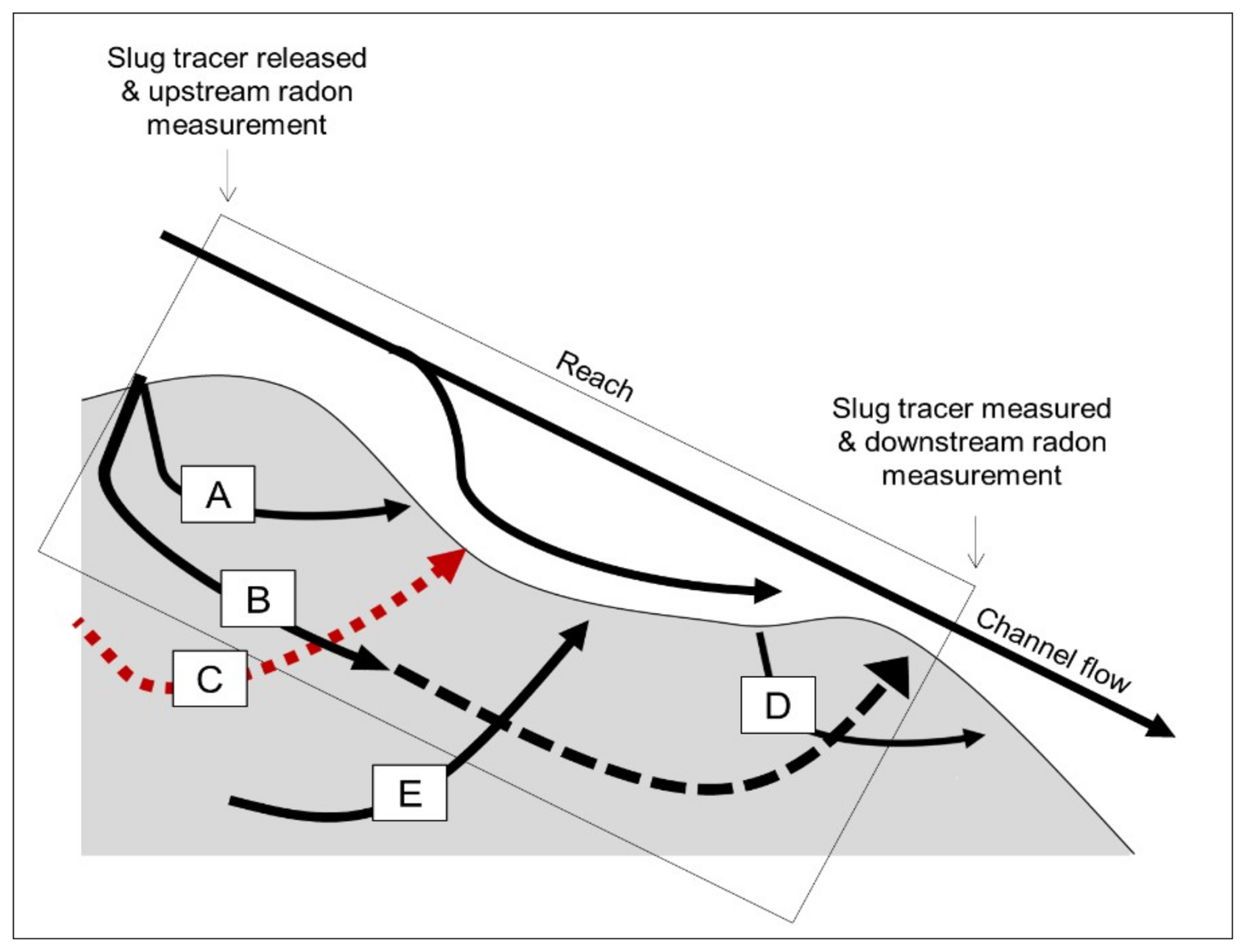
Figure 9 Conceptual figure of flow paths in streams. The box shows the reach of investigation. A is a flow path that is labelled by the tracer at the upstream location and returns within the WoD. B is a flow path with timescales longer than the WoD, where transit times exceed the duration of the tracer experiment, as indicated by the dashed arrow. C is a subsurface flow path entering the hyporheic zone upstream of the reach. This flow path is characterized by subsurface transit times shorter than 21 d and radon activity that has not yet reached secular equilibrium. This flow path can be identified by radon but not by chloride concentration, which explains the red coloration. D is a flow path that bypasses the downstream end of the reach. E is a groundwater flow path with transit times longer than 21 d and radon activity at secular equilibrium. Flow path C is conceptually excluded from the TSM, which is why it is highlighted with a red dashed arrow (Figure adapted from Payn et al., 2009).

4.4 Implications and future research

The improved parameter identifiability through joint TSM calibration with radon and chloride may be a critical step toward enhancing the physical realism of TSMs and providing more reliable estimates of solute transport. This is important because past studies found that the relationships between TSM parameters and hydrologic drivers are often contradictory (Ward and Packman, 2019; Bonanno et al., 2022). We envision that future studies will derive model parameters by jointly calibrating TSMs across diverse environments and hydrologic conditions. This approach can help clarify how model parameters vary with hydrologic drivers. To advance this goal, studies should compare streams across varying scales and geological settings to determine how these differences affect calibration outcomes when radon is included. Through such comparative studies, researchers could test our expectation that streams with higher radon activity, typically smaller-order streams with granite-rich geology, will yield greater certainty for groundwater inflow q_I and improved model performance when TSMs are jointly calibrated with radon and chloride. This greater certainty for q_I might result from the larger difference in radon concentration activity between groundwater and stream water. Furthermore, future research could jointly calibrate TSMs with radon and tracer data from constant rate injections. This approach would test whether radon captures temporally longer flow paths than those detected by constant rate but not by slug tracer injections.

For future research with radon on gross exchange fluxes, we recommend constraining the transient storage parameter by considering surface (e.g., pools) and subsurface transient storage zones (e.g., hyporheic zones) in TSM evaluations (e.g., Choi et al., 2000). This distinction might be critical because only surface storage contributes to radon degassing, whereas radon activity increases mainly in the subsurface storage and, to a lesser extent, in surface storage. These storage-specific processes are not fully captured by using a single storage zone, as implemented in OTIS-R, instead of two. We selected the one-zone storage model because this setup aligns conceptually with most established radon models (e.g., Cook et al., 2006; Frei and Gilfedder, 2015) and many TSM calibration with slug tracers (e.g., Bonanno et al., 2023). To our knowledge, no prior radon study has considered two storage zones, highlighting a promising opportunity for future research. We also recommend incorporating additional discharge measurements to reduce measurement errors. This is important because the calibrated gross exchange fluxes for Oak Creek fall within the confidence interval of changes in net discharge (Fig. 8). Therefore, caution is needed when interpreting these fluxes. By following these recommendations, future studies may unlock radon's full potential as a tracer. This will enable deeper insights into the continuum of subsurface flow paths beyond the WoD of slug tracer injections. Experimental setups could, for instance, measure radon activity alongside BTCs at several downstream locations from the point of injection (e.g., Ward et al., 2023), thereby supporting the assessment of large spatial-scale subsurface flow paths from slug tracer injections. Studies focusing on understanding the turnover of chemical compounds along large spatial-scale subsurface flow paths could benefit from incorporating radon as an additional tracer. This is especially relevant for slower chemical degradation processes, such as denitrification, which are more likely to occur along flow paths with longer timescales (sensu Jimenez-Fernandez et al., 2022) which radon may help resolve.

5 Conclusions

The goal of this study was to quantify flow paths of different timescales at the reach scale using measurements of chloride concentration and naturally occurring radon. To achieve this, we calibrated a transient storage model (TSM) with each tracer individually and with both jointly. Our results show that TSM calibration with chloride yields identifiable, narrower parameter values, while calibration with radon does not result in identifiable parameters. The lack of identifiability with radon is due to steady-state activity of radon in the stream, the tracer's sensitivity to the amount and location of groundwater inflow, and to large-scale subsurface flow paths, demonstrating radon's bias toward flow paths with longer temporal timescales. We found that joint calibration of a TSM with both tracers provided the most information on parameters of the TSM compared to calibrating it with either tracer alone. Based on these findings, we recommend that future studies incorporate both radon and chloride when calibrating the TSM to improve estimates of solute transport. Furthermore, with an adapted sampling and modeling strategy, we see significant potential in incorporating radon in future studies to unlock its full potential in revealing flow paths with longer timescales than those traced by slug tracer injections.