Thermobaric circulation induced by cabbeling in a deep freshwater lake: a conceptual 1D model

Numerical lake models are a powerful tool to optimize water management and mitigate changes due to climate change. Hence, detailed implementation of lake specific processes is crucial to ensure optimal results. However, common numerical lake models have so far omitted the effect of thermobaricity despite its significant influence on deep water circulation in deep lakes. The thermobaric effect is based on the temperature dependence of the compressibility of water. As a consequence, deep water can be significantly colder than 4 °C and deep water renewal becomes complex. For a proper investigation, numerical models can be appropriate tools to display and understand such processes better. Inspired by Lake Shikotsu, which is an excellent example for the influence of thermobaricity, we developed a simplified 1D model for thermobaric effects. Here, we used in situ density to replace potential density for stability considerations such as the Brunt-Väisälä frequency. To prevent any competing influences and isolate thermobaric effects, we excluded any external forcing except for the surface temperature input. Accordingly, we excluded salinity, chose a cylindrical bathymetry without shallow areas, and omitted any inflows. Therefore, the model reproduced deep water circulation solely based on thermal forcing at the surface. We were able to identify key features of the deep water circulation: (1) cabbeling occurs at the intersection of the temperature profile with the T_md (temperature of maximum density) line due to diffusion and induces thermobaricity driven deep water circulation, (2) this deep water circulation cell is detached from the surface, but can extend over hundreds of meters to the lake bed, (3) the deep water stays isothermal, (4) and after the winter stratification the temperature profile aligns with the T_md line. Additionally, we investigated the influence of previous deep water renewal events and the current surface temperature on the deep water circulation. Our results emphasize the feasibility and necessity of the implementation of thermobaricity in numerical lake models by basing stability (Brunt-Väisälä frequency) on in situ density.

1 Introduction

Across all climate zones, lakes and reservoirs are undergoing changes due to climate change (Adrian et al., 2009; Sun et al., 2025) and heavy human impact (Søndergaard and Jeppesen, 2007; Weyhenmeyer et al., 2024). These water bodies provide central services such as water and food supply, energy production, flood prevention, and space for recreation. In particular, the provision of high quality drinking water is becoming an increasing challenge that humanity has to deal with (Delpla et al., 2009). This accounts globally and awareness is growing. Hence, to ensure optimal management of lakes and reservoirs in the future, proper knowledge of processes and the prediction of changes are crucial. Numerical modeling of lakes serves as a central tool to predict future development and optimize management strategies (e.g. Weber et al., 2019; Mi et al., 2022) to restore and maintain a healthy ecological state of our natural environment. Good management can help adapt our strategies and mitigate the influences of climate change and direct human impact at least in part (e.g. Winton et al., 2019; Regev et al., 2025).

Numerical models for lakes are often based on assumptions originating from oceanography. As a consequence, the inclusion of lake specific properties of limnic waters can improve simulations of lakes fundamentally. This spans from using local weather conditions to implementing lake specific solute compositions in density functions (Pawlowicz and Feistel, 2012; Moreira et al., 2016). In this paper, we want to demonstrate the necessity of including the temperature dependence of the compressibility in the water properties, which is called thermobaricity (McDougall, 1987). Thermobaricity has so far not been dealt with in the commonly used lake models. However, some ocean models changed to in situ density when they changed to the new ocean standard TEOS-10 (IOC et al., 2010), which includes the effect.

The effect of thermobaricity is based on the temperature dependence of the compressibility of water (which is tantamount to the pressure dependence of the thermal expansion of water, ${\partial }^{\mathrm{2}}{\mathit{\rho }}_{\text{in-situ}}/(\partial \mathit{\theta }\partial p)$) (McDougall, 1987). For pure water, this leads to a decrease of the temperature of maximum density T_md from approximately 3.98 °C at atmospheric pressure by about 0.02 °C bar⁻¹ (Chen and Millero, 1977). For instance, pure water at the pressure of 500 m depth has its temperature of maximum density at about 3 °C. Ultimately, water colder than 3.98 °C is less dense than slightly warmer water at the surface but denser from a certain depth where T_md is low enough. As a consequence, we find deep water significantly colder than 3.98 °C in deep lakes of the temperate climate zone (e.g. Carmack and Weiss, 1991; Crawford and Collier, 1997; Boehrer et al., 2009, 2013; Carmack and Vagle, 2021; Carmack et al., 2024).

Also connected to the temperature of maximum density, the process of cabbeling differs from thermobaricity (McDougall, 1987; Carmack and Weiss, 1991; Grace et al., 2023a, b). Cabbeling occurs where mixing of two water parcels across the temperature of maximum density results in even denser water, which itself drives convective circulation, e.g. in the case of thermal bars (Ivey and Hamblin, 1989; Shimaraev et al., 1993). Although deep water renewal in deep lakes experiencing surface water temperatures below 3.98 °C is controlled mainly by thermobaricity, also cabbeling may be involved in the deep mixing and deep water formation.

The vertical progression of cold surface water to the abyss is complex and the depiction of density differences becomes difficult as the convenient property of potential density, namely having one reference pressure, is lost when thermobaricity is dealt with. For proper stability considerations, the densities of two vertically separated water parcels need to be compared at intermediate identical pressure conditions, i.e. at the pressure at which the two water parcels are and interact (Ekman, 1934). For this, the adiabatic change of the water parcels from their origin towards the comparison pressure has to be considered (Osborn and LeBlond, 1974). We show that using in situ density for stability considerations including thermobaricity is a proper approach if this adiabatic change is considered.

External forcing by strong winds as driving force for the deep water renewal has been discussed (e.g. Weiss et al., 1991; Boehrer et al., 2013). Here, these winds push cold water beyond the compensation depth, where it becomes denser than the ambient water, and from there it can proceed sinking due to its higher in situ density up to a depth with equally dense water. Killworth et al. (1996) and Piccolroaz and Toffolon (2013) created models to describe such deep water renewal in Lake Baikal. They used wind as external forcing to represent downwelling under conditions of thermobaricity. While Killworth et al. (1996) used a two dimensional model to include the wind in combination with a one dimensional model for vertical tracer distributions, Piccolroaz and Toffolon (2013) parametrized the wind forcing to calculate the forced downwelling before assessing the stability. In contrast to them, we excluded forced plume downwelling while allowing for cabbeling to present the existence of thermobaricity controlled deep water mixing that is purely one dimensional and not driven by wind. Additionally, we wanted to emphasize the possibility of directly using in situ density for stability considerations to include thermobaricity in lake models by comparing two water parcels at a common depth. Piccolroaz and Toffolon (2013) also used a common depth for comparison but only considered the adiabatic change in in situ temperature, while we could avoid this additional calculation by referring to potential temperatures only.

In our model, we wanted to ensure that there was no interference of other effects with the effects of thermobaricity and no misinterpretation of thermobaric effects as secondary effects of other driving forces. Therefore, we decided to keep everything at the minimum complexity to depict the thermobaric effects as well isolated as possible. Consequently, we considered a cylindrical water domain without lateral gradients (on the considered length scale) for our 1D model. We prohibited shallow areas for the formation of waters of different properties, valleys to guide submerged flows, horizontal gradients at the surface, and geothermal heating at the bottom. Additionally, we implemented pure water properties (no salinity). Lake Shikotsu, Hokkaido, Japan, served as our inspiration, because thermobaric stratification has been documented there (Boehrer et al., 2008, 2009). Hence, we chose the temperature range and size of the basin accordingly, hoping that our numerical 1D model would manage to reproduce water circulation patterns and temperature profiles with some similarities to Lake Shikotsu. As we had presumed that the deep water circulation in this lake could be understood as a one dimensional circulation, we believed that our parsimonious model should represent the fundamental features there. Nevertheless, we did not expect too close similarity, since we abstained from including any detailed information of bathymetry or forcing. Even though Lake Shikotsu is a particularly nice representation of thermobaricity and the necessity of including this effect is obvious, we hope to convince the readers of the importance of including temperature dependent compressibility (thermobaricity) in numerical models, if they want to have a realistic simulation of deep water movements in lakes with deep water temperatures close to the temperature of maximum density.

2 Methods

2.1 Inspiration

Our 1D model was inspired by Lake Shikotsu, Hokkaido, Japan. This lake is located in the temperate zone and consistently experiences surface water temperatures below 3.98 °C during winter. It is a volcanic caldera lake of collapse type, formed by the great eruption of Shikotsu Volcano about 40 000 years ago. Because of that, the lake has a roughly cylindrical shape, very steep sidewalls, and a maximum depth of 360 m (Fig. 1a). Boehrer et al. (2008, 2009) investigated the deep water circulation and its dependency on thermobaricity. The temperature profiles, measured in 2005, clarify this dependency (Fig. 1b). They cross the T_md line during the winter stratification and resemble the T_md line above this intersection shortly after the end of the winter stratification. At the same time, the deep water temperature below the intersection stays isothermal throughout. The conductivity profiles are also presented (Fig. 1c). The very steep sidewalls and comparatively small horizontal extent of the lake, as well as its symmetric shape, suggest a rather one dimensional governance of the system. Missing shallow areas along the shore and the uniform slope without any trenches make the accumulation and downwelling of cold water plumes induced by external forcing unlikely.

Figure 1 Location, bathymetry, potential temperature, and conductivity profiles from 2005 of Lake Shikotsu. (a) shows the location of Lake Shikotsu in Japan (red dot), (b) presents the bathymetry map of Lake Shikotsu (created by editing GSI (Geospatial Information Authority of Japan) Tiles (https://maps.gsi.go.jp/development/ichiran.html#lake, last access: 23 October 2025)), (c) shows potential temperature profiles from 2005 and the temperature of maximum density T_md, and (d) electrical conductivity profiles normalized to 4 °C (compare Boehrer et al., 2009) for the same dates as in (c) (data from Boehrer et al., 2008, 2009).

2.2 Density and stability

The density of water parcels can be calculated at every pressure and is referred to as in situ density ${\mathit{\rho }}_{\text{in-situ}}={\mathit{\rho }}_{\text{in-situ}}\left(T,p\right)$ in this paper. If a parcel is moved adiabatically to a different reference pressure than its current position one can speak of potential density ρ_pot=ρ_pot(T). In general, ${\mathit{\rho }}_{\text{in-situ}}\left(T,p_{\mathrm{ref}}\right)={\mathit{\rho }}_{\mathrm{pot}}\left(T\right)$ holds for a given reference pressure p_ref if the used formulation accounts for the compressibility and its temperature dependency and uses potential temperature to account for the adiabatic change. In this paper, we follow the usual oceanographic and limnological practice of defining ρ_pot at atmospheric pressure (though sometimes other pressure references have been recommended for use, e.g. Ekman, 1934; Osborn and LeBlond, 1974).

To start with, the sound speed c is directly connected with the compressibility of water β_S by

$$\begin{array}{}\text{(1)}& {\mathit{\beta }}_{\mathrm{S}}={\displaystyle \frac{\mathrm{1}}{{\mathit{\rho }}_{\text{in-situ}}}}{\left({\displaystyle \frac{\partial {\mathit{\rho }}_{\text{in-situ}}}{\partial p}}\right)}_{\mathrm{S}}={\displaystyle \frac{\mathrm{1}}{{\mathit{\rho }}_{\text{in-situ}}\cdot c^{\mathrm{2}}}}\end{array}$$

(Meschede, 2015), where p is the pressure and the index S indicates an adiabatic process, and therefore represents the temperature dependency of the compressibility (thermobaricity). Hence, we used this to obtain a formulation of the in situ density. According to Eq. (1), the sound speed can be expressed by

$$\begin{array}{}\text{(2)}& {\displaystyle \frac{\mathrm{1}}{c^{\mathrm{2}}}}={\left({\displaystyle \frac{\partial {\mathit{\rho }}_{\text{in-situ}}}{\partial p}}\right)}_{\mathrm{S}}.\end{array}$$

From Eq. (2) the in situ density can be derived as

$$\begin{array}{}\text{(3)}& {\mathit{\rho }}_{\text{in-situ}}={\mathit{\rho }}_{\mathrm{pot}}+\underset{\mathrm{0}}{\overset{p}{\int }}{\displaystyle \frac{\mathrm{1}}{c^{\mathrm{2}}}}\mathrm{d}p.\end{array}$$

Here, in situ density and sound speed depend on temperature, salinity, and pressure while potential density, here with the reference pressure of 0 bar at the water surface, only depends on temperature and salinity. In our approach, we exclude salinity to prevent distraction by competing effects. Hence, salinity is disregarded in the following and we use the formulations of Tanaka et al. (2001) for potential density and Belogol'skii et al. (1999) for sound speed. We are fully aware that for limnic water the solutes must be included in the water properties for the calculation of density (Boehrer et al., 2010; Moreira et al., 2016) and sound speed when salinity is considered for a fully realistic representation.

Equation (3) is then further simplified by applying a linear approximation for $\frac{\mathrm{1}}{c^{\mathrm{2}}}$ with respect to pressure

$$\begin{array}{}\text{(4)}& {\displaystyle \frac{\mathrm{1}}{c^{\mathrm{2}}\left(p\right)}}=mp+n,\mathrm{with}m={\displaystyle \frac{\partial \frac{\mathrm{1}}{c^{\mathrm{2}}\left(p\right)}}{\partial p}}\mathrm{and}n={\displaystyle \frac{\mathrm{1}}{c^{\mathrm{2}}\left(p=\mathrm{0}\right)}}.\end{array}$$

We used the surface and bottom values for linearization of the modeled depth range up to 360 m (compare Sect. 2.3). Hence, the maximum deviation occurs at mid depth, regardless of the temperature. For the interesting temperature range close to the temperature of maximum density T_md, between 3 and 4 °C, a maximum deviation of $\mathrm{2.13}\times {\mathrm{10}}^{-\mathrm{12}}{\mathrm{s}}^{\mathrm{2}}{\mathrm{m}}^{-\mathrm{2}}$ of the sound speed occurs for 3 °C. This deviation is small relative to the change of $\frac{\mathrm{1}}{c^{\mathrm{2}}}$ with respect to temperature or pressure, which are in the order of ${\mathrm{10}}^{-\mathrm{9}}{\mathrm{s}}^{\mathrm{2}}{\mathrm{m}}^{-\mathrm{2}}$.

The final formulation of the in situ density is

$$\begin{array}{}\text{(5)}& {\mathit{\rho }}_{\text{in-situ}}\left(T,p\right)={\mathit{\rho }}_{\mathrm{pot}}\left(T\right)+{\displaystyle \frac{p^{\mathrm{2}}}{\mathrm{2}}}{\displaystyle \frac{\partial \frac{\mathrm{1}}{c^{\mathrm{2}}\left(T,p\right)}}{\partial p}}+{\displaystyle \frac{p}{c^{\mathrm{2}}\left(T,p=\mathrm{0}\right)}}.\end{array}$$

While we clearly distinguish between ρ_in-situ(T,p) and ρ_pot(T), we only use potential temperature T (and never in situ temperature T_in-situ; differences would be in the range of 1 mK in the presented case). In this case, potential temperature is the appropriate quantity to use due to the used density formulation. Also, the differences to conservative temperature as used in TEOS-10 are small in the interesting temperature range and there is essentially no production of potential temperature during mixing when salinity is excluded (compare Fig. 2a in McDougall, 2003).

With the explicit formulation of the in situ density it is now possible to compare neighbouring water parcels at the same pressure to check for density differences. Similarly, the Brunt-Väisälä frequency of a displaced water parcel can be calculated by subtracting the adiabatic density change due to pressure changes from the water column (in situ) density gradient: the Brunt-Väisälä frequency is positive (the water column is stable) when the adiabatic density change of the displaced water parcel exceeds the surrounding water column (in situ) density change (Peeters et al., 1996). This is done straight forward by using the in situ density as

$$\begin{array}{}\text{(6)}& \begin{array}{rl}{N}^{\mathrm{2}}& =-{\displaystyle \frac{g}{{\mathit{\rho }}_{\text{in-situ}}}}\cdot \left({\displaystyle \frac{\partial {\mathit{\rho }}_{\text{in-situ}}}{\partial z}}-{\displaystyle \frac{\partial {\mathit{\rho }}_{\text{in-situ}}}{\partial p}}{\displaystyle \frac{\partial p}{\partial z}}\right)\\ & =-{\displaystyle \frac{g}{{\mathit{\rho }}_{\text{in-situ}}}}{\displaystyle \frac{{\mathit{\rho }}_{\text{in-situ}}\left(T_{i+\mathrm{1}},p_{i+\mathrm{1}}\right)-{\mathit{\rho }}_{\text{in-situ}}\left(T_i,p_{i+\mathrm{1}}\right)}{z_{i+\mathrm{1}}-z_i}},\end{array}\end{array}$$

where z is the depth and the indices indicating the layer of the quantity of the corresponding water parcel. Hence, the adiabatic compensation of the pressure difference formally results in comparing ρ_in-situ of the two water parcels at a common local pressure, which is known as the adiabatic leveling method (Bray and Fofonoff, 1981; Millard et al., 1990). For simplicity, we chose the depth of one of the water parcels as common pressure.

2.3 Numerical model

We created a simple 1D model to conceptually simulate deep water circulation under consideration of thermobaricity. The model domain consisted of 180 layers of 2 m each, which resulted in a maximum depth of 360 m. The values were motivated by Lake Shikotsu because this kind of deep water renewal is suspected to have a significant influence in this lake (compare Fig. 1c). The lateral extent of the layers was not specified, but the volume and hence the horizontal extent of all layers was considered equal. Lateral gradients were excluded by the one dimensional design of the model domain (Boehrer et al., 2008) and no exchange of the water column with the lake bed was assumed. The model started with an homogeneous temperature profile.

Our intention was the demonstration of thermobaricity. Hence, in contrast to common lake models, we removed the atmospheric forcing at the lake surface. Instead, we used surface water temperature as a (Dirichlet) boundary condition (Boehrer et al., 2000) while we did not allow any exchange at the lake bottom (no-flux boundary condition) to exclude geothermal heating and subsurface flows. As a consequence, the numerical model was exclusively forced by temperature, and resulting density differences, in the surface layer of the model. The exclusion of other driving forces prevented their interference with and the misinterpretation of thermobaricity driven effects.

In the model, each time step consisted of (1) setting the surface temperature to the prescribed surface temperature input, (2) diffusion through the water column, and (3) a stability check and resulting mixing in this specific order.

2.3.1 Surface temperature input

First for each time step, the surface temperature was set to the surface temperature input. As input, the annual surface temperature from Lake Shikotsu was repeated over seven years which is the total length of the simulation. To include the effect of day-night variation, the time step was set to 1 h. The surface temperature from Lake Shikotsu was measured at a depth of about 1.5 m with one measurement every minute from 18 October 2023 to 8 May 2024 with a temperature sensor RBRsolo³ T (RBR, Canada), which includes temperatures significantly colder than 4 °C during the winter (compare Fig. 3). We decided to use real surface data to keep heat exchange with the atmosphere in a realistic range. The surface temperature series was then linearly interpolated from May 2024 to October 2023 to a duration of one year and then repeated over seven years. Although surface temperatures during the summer are unrealistically represented by the linear interpolation, the thermobaric effect is unaffected by temperatures above 4 °C and the summer temperatures are much warmer.

2.3.2 Turbulent diffusion

Turbulent diffusion was applied on the water column to account for general small scale water movements. We chose a constant value for the whole water column to ensure that interference with the circulation pattern is not possible. To include turbulent diffusion while keeping the model processes as simple as possible we chose a simple volume exchange method. This was realized by exchanging half of the volume of each layer equally with both neighbouring layers (one quarter up, one quarter down) and homogenizing each layer correspondingly, which is described for temperature as

$$\begin{array}{}\text{(7)}& T_{t,i}={\displaystyle \frac{\mathit{\nu }}{\mathrm{2}}}{T}_{t-\mathrm{1},i-\mathrm{1}}+\left(\mathrm{1}-\mathit{\nu }\right)T_{t-\mathrm{1},i}+{\displaystyle \frac{\mathit{\nu }}{\mathrm{2}}}{T}_{t-\mathrm{1},i+\mathrm{1}},\end{array}$$

where the indices indicate the corresponding timestep and layer, respectively, and ν being the exchange fraction, the exchanged part of the volume of each layer. This exchange results in a diffusivity of $D\left(\mathit{\nu }\right)=\frac{l\cdot \mathrm{0.5}\mathit{\nu }l}{t}$ (Eq. A4, see Appendix A). Hence, the amount of diffusion can be controlled by the time step size t, layer size l, and the prescribed exchange fraction. Also, the stability criterion for explicit diffusion schemes $D<\frac{\mathrm{1}}{\mathrm{2}}\frac{{\left(\mathrm{\Delta }x\right)}^{\mathrm{2}}}{\mathrm{\Delta }t}$, here Δx=l and Δt=t, holds for $\mathrm{0}<\mathit{\nu }<\mathrm{1}$. For the value used (v=0.5), the scheme implements a diffusion of about $\mathrm{2.7}\times {\mathrm{10}}^{-\mathrm{4}}{\mathrm{m}}^{\mathrm{2}}{\mathrm{s}}^{-\mathrm{1}}$ (estimated with Eq. A4), which is roughly in the expected order of magnitude (e.g. Saber et al., 2018) and similar to values used in other model studies of thermobaric deep water circulation (Piccolroaz and Toffolon, 2013; Wood et al., 2023). For more details on the chosen diffusivity and its limitations see Appendix A and Sect. 4.2, respectively.

2.3.3 Stability check

After the diffusion was applied in each time step, the water column was checked for stability. The water column was regarded as stable if the in situ density gradient was larger than the adiabatic change of the in situ density

$$\begin{array}{}\text{(8)}& {\displaystyle \frac{\partial {\mathit{\rho }}_{\text{in-situ}}}{\partial z}}>{\left({\displaystyle \frac{\partial {\mathit{\rho }}_{\text{in-situ}}}{\partial z}}\right)}_{\mathrm{S}}\end{array}$$

(Peeters et al., 1996). With discretization this criterion condenses to

$$\begin{array}{}\text{(9)}& {\mathit{\rho }}_{\text{in-situ}}\left(T_{i+\mathrm{1}},p_{i+\mathrm{1}}\right)>{\mathit{\rho }}_{\text{in-situ}}\left(T_i,p_{i+\mathrm{1}}\right),\end{array}$$

again a comparison at the pressure of the lower layer. Equation (9) is used to compare neighbouring layers locally and check for stability, where we added a very small threshold of ${\mathrm{10}}^{-\mathrm{9}}\mathrm{kg}{\mathrm{m}}^{-\mathrm{3}}$ to prevent small mixing artifacts during stable summer stratification. This stability check is similar to the stability algorithm used by Piccolroaz and Toffolon (2013) except that we directly calculate densities at the same pressure with potential temperature instead of calculating the change in in situ temperatures and then calculating the densities. Equation (9) is iteratively applied bottom up. If the stratification is stable, there is no action and the next upper layer is checked. However, if water in the lower layer is less dense than in the upper, the layers are mixed and the temperatures of the two layers are averaged. The mixed layers are then iteratively compared and mixed with all layers below in the water column until they are stable again. Then again, the next upper layer is checked. If the layers are unstable up to the temperature controlled surface layer, the temperatures of all corresponding layers are set to the prescribed surface temperature. By doing so, all instabilities are removed over the whole water column in each time step.

2.3.4 Model workflow

For demonstration, Fig. 2 illustrates the operation of the model processes on an exemplary winter temperature profile for one time step. While convection driven by surface temperature has widely been dealt with we focus for now on the region where the temperature profile intersects with the T_md line. After setting the uppermost layer onto the surface temperature (1), turbulent diffusion mixes the water column (2). Close to T_md, where the temperature profile intersects the T_md line, the temperature profile T_t=1 changes to T_t=2 due to diffusion. The temperature in layer i is now closer to T_md than before: $T_{\mathrm{md}}<T_{\mathrm{2},i}<T_{\mathrm{1},i}$ (vertical cabbeling since $T_{\mathrm{1},i-\mathrm{1}}<T_{\mathrm{md},i}<T_{\mathrm{1},i}=T_{\mathrm{1},i+\mathrm{1}}$). Next, the water column is checked for stability and mixed (representing convection) if unstable (3). Coming from temperature profile T_t=2, the water column is unstable for layer i and i+1, since $T_{\mathrm{md},i+\mathrm{1}}<T_{\mathrm{2},i}<T_{\mathrm{2},i+\mathrm{1}}$ compared at layer i+1, and they are mixed. The same condition holds for the next layer below compared to the temperature of the mixed layers and so on. Eventually, the isothermal lower water column is mixed to the bottom (or a certain depth where lower temperatures are present in the temperature profile T_t=2) and the temperature profile T_t=3 has developed. At the same time, conventional instabilities at the surface are erased as well. It should be noticed, that the model does all stability calculations with the densities as explained above. Interestingly, the heat transport through the T_md line results in a stabilizing effect above and a destabilizing effect below T_md.

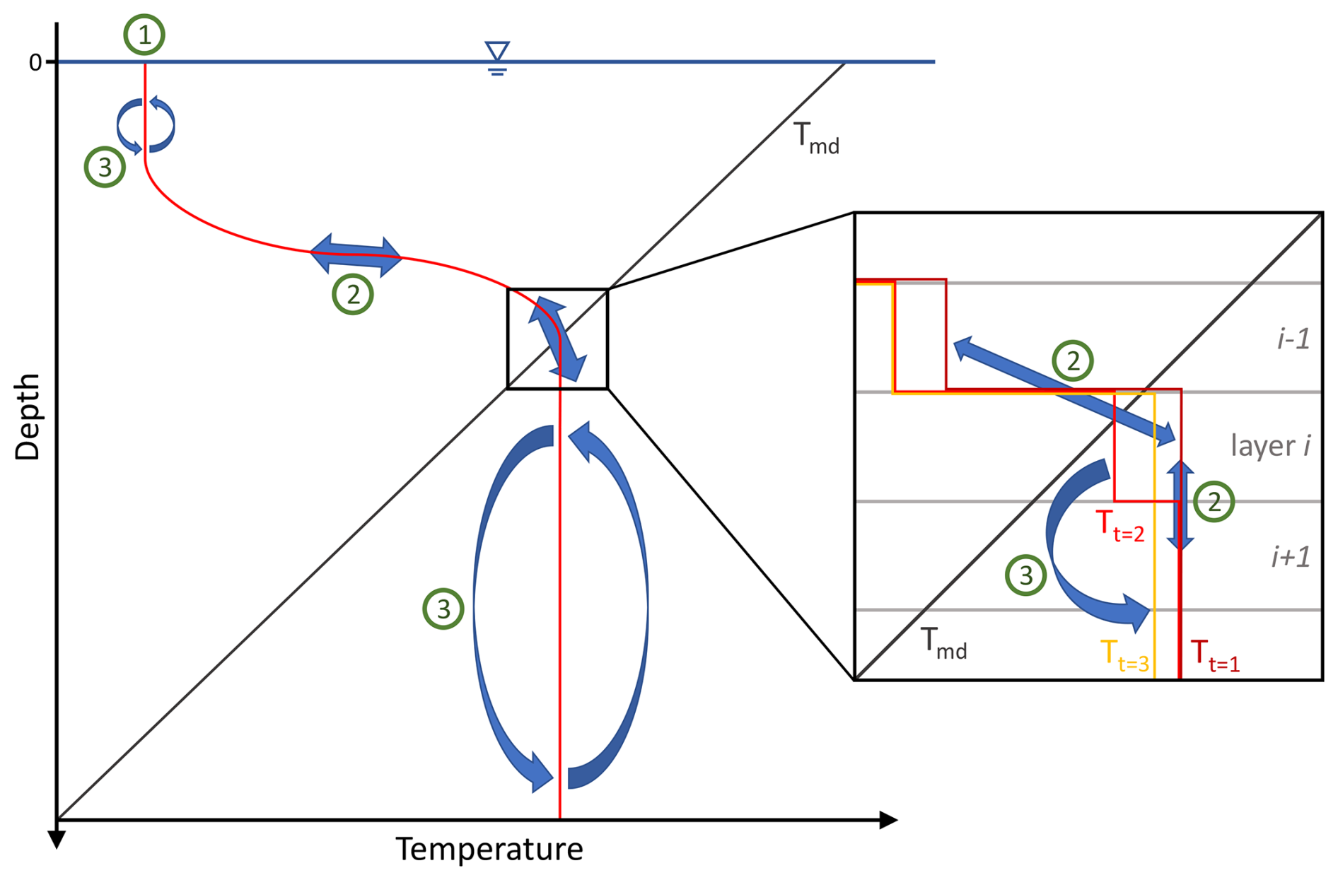
Figure 2 Model processes operating on an exemplary winter temperature profile during one time step. The processes of controlling the surface temperature (1), turbulent diffusion (2), and mixing due to instability (3) are numbered in the order they occur. The zoomed in window shows the temperature profile at the intersection with the T_md line between (1) and (2): T_t=1, (2) and (3): T_t=2, and after (3): T_t=3. For a detailed description see the text.

We demonstrated the model processes using the temperature profiles instead of potential or in situ density, because the densities are both not suitable for visualization. Potential density would always refer to a non-local, usually atmospheric, pressure which would not indicate changes in the stability due to pressure effects. In situ density is depicting the pressure influence and the small changes in the temperature after mixing only induce hardly visible changes in the gradient of the in situ density. In contrast to that, using temperature profiles in combination with depicting the T_md line readily enables illustrating instabilities. Also, the temperature is the key driver for this type of deep convection.

To demonstrate that thermobaric conditions form from an isothermal starting profile of 4.2 °C and remain thereafter, we ran the model for seven years. Hence, we can use later years when thermobaric conditions have established to discuss the resulting circulation features. In addition, two more runs were done by changing the input surface temperature in the fourth year by adding and subtracting 0.4 °C, respectively. They provide an impression of the stability of thermobaricity and the effect of variable winters on deep water renewal.

3 Results

The model is driven by the input of the surface temperature. We follow the ocean convention of referring to hydrostatic pressure of 0 bar at the water surface. The simulated temperatures at mid depth (18 bar) and the bottom (35 bar) are also displayed for the entire simulation time (Fig. 3). At mid depth, the temperature rises during the summer stratification and follows the surface temperature to a temperature slightly below 4 °C during autumn and winter indicating deep water circulation. This temperature is also equal to the temperature at 35 bar, where only little temperature variation can be observed during the simulation except for the first winter, because the starting temperature profile was set to 4.2 °C.

Figure 3 Temperature logs at different depths. The logs show the temperature progression of the controlled surface temperature (0 bar) and at depths of 18 and 35 bar over the entire simulation period.

3.1 Temperature profiles

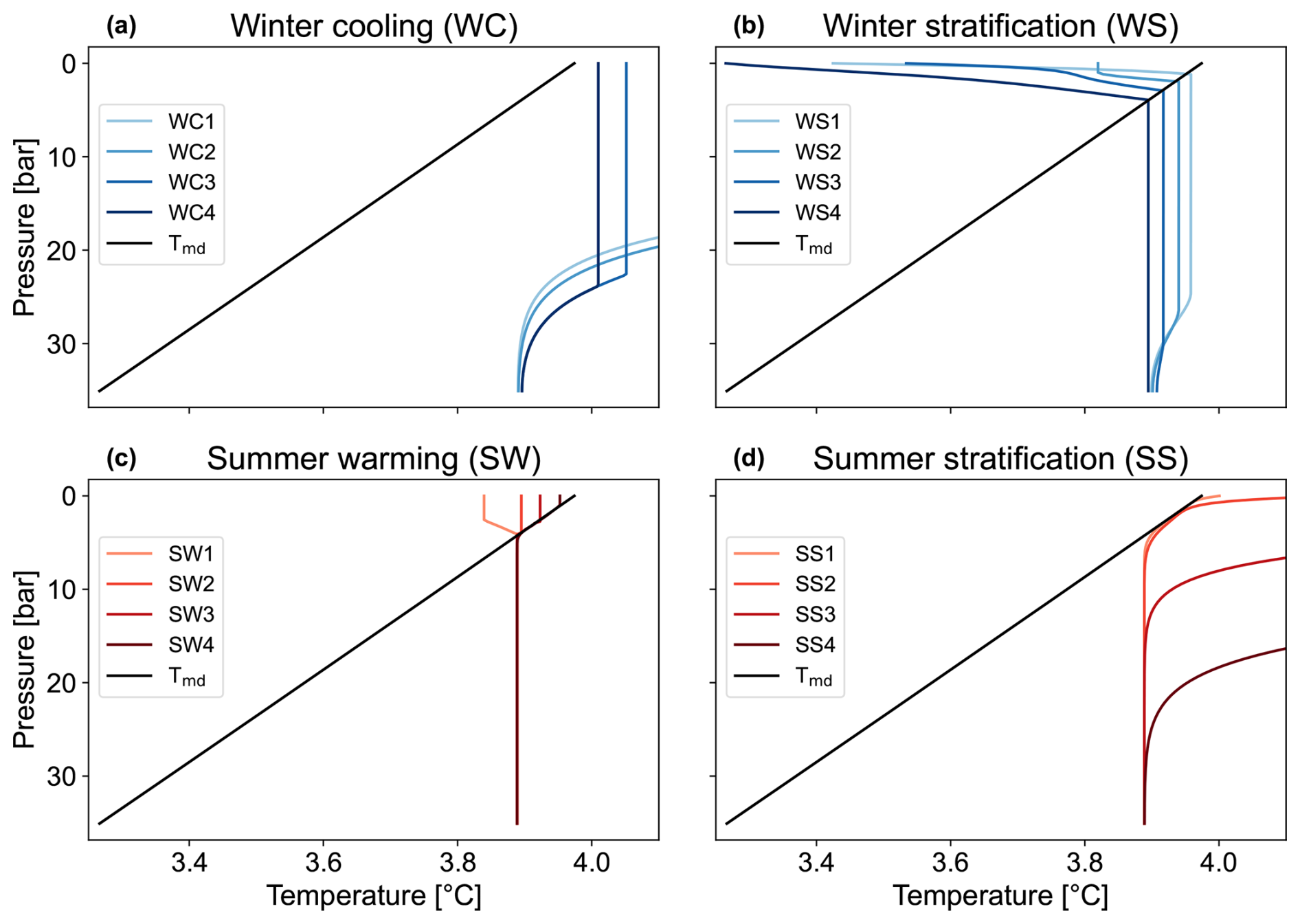
For the discussion of typical thermobaric circulation features, we refer to the fourth year of simulation, as we considered the first three years as possibly affected by the initial conditions. We divide the year into typical stratification phases: winter cooling (WC), winter stratification (WS), summer warming (SW) and summer stratification (SS). The order of these phases is oriented on the starting point of the simulation, which is in October, the beginning of the measured surface temperature input. Figure 4 exhibits four exemplary temperature profiles for each phase.

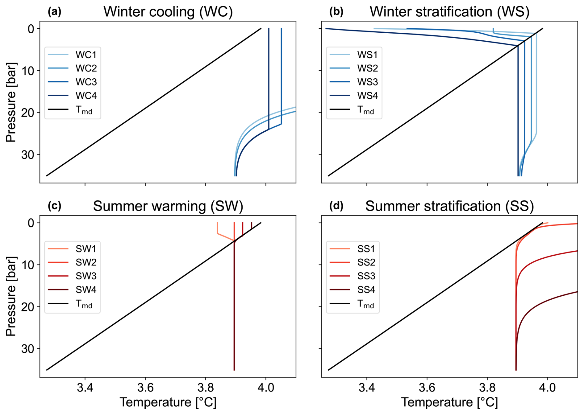
Figure 4 Temperature profiles of the fourth year of the simulation period. The selected temperature profiles are split into four plots for clarity. (a) contains profiles from the winter cooling (WC) phase, (b) from the winter stratification (WS) phase, (c) from the summer warming (SW) phase, and (d) from the summer stratification (SS) phase. Their points in time are marked in Fig. 5. Additionally, all plots include the temperature of maximum density T_md.

The four exemplary profiles of the winter cooling (WC1: 12 November, 20:00 UTC; WC2: 29 November, 12:00 UTC; WC3: 7 January, 01:00 UTC; WC4: 7 January, 10:00 UTC) are shown in Fig. 4a. During this phase, the surface water cools rapidly and circulates the water below to a depth where colder temperatures still stabilize the water column. Additionally, due to the high surface temperatures compared with the deep water temperatures, the deep water is still subject to warming (compare WC1 and WC2 with WC3 and WC4). This behavior continues until the surface water reaches the temperature of maximum density T_md at the surface, which is approximately 3.98 °C. From that point on, the inverse winter stratification begins.

During the winter stratification, the surface water is further cooled and it stratifies inversely (compare profiles in Fig. 4b: WS1: 21 January, 14:00 UTC; WS2: 29 January, 07:00 UTC; WS3: 20 February, 14:00 UTC; WS4: 19 March, 16:00 UTC). This means that close to the surface colder water floats on warmer water due to its lower density. Inverse stratification is stable to the point where the temperature profile intersects the T_md line. Here, water mixes across T_md due to diffusion and produces denser water (Grace et al., 2023a, b). This diffusion induced cabbeling can only occur because of the change of T_md with depth, i.e. thermobaricity. The denser water then circulates the water column below due to thermobaricity to the depth where lower temperatures stabilize the water column. Since the surface water is further cooled in this phase, cold temperatures diffuse downwards to the intersection with T_md. This deepens the intersection and ever colder water mixes into the deep water. Eventually, the bottom layer is replaced by colder water from above and the circulation extends to the deepest point. Hence, the intersection with T_md controls the deep water temperature. Short intermediate warming events at the surface (e.g. WS2) induce small mixing cells at the surface, similar to the winter cooling, but do not influence the deep water mixing cells or their progression. The winter stratification comes to an end when the surface temperature starts to rise significantly.

During the summer warming (profiles in Fig. 4c: SW1: 2 April, 20:00 UTC; SW2: 3 April, 09:00 UTC; SW3: 3 April, 13:00 UTC; SW4: 3 April, 21:00 UTC) the inverse stratification gets erased by the rising surface temperatures. Since the surface layer temperature is below 3.98 °C, the warming surface water mixes the colder water below due to the higher density and we see a homogenized surface layer. From the moment when the surface layer temperature exceeds the deep water temperature (SW2), cabbeling comes to an end. The circulation of the deep water stops and a stable density stratification establishes along T_md above the isothermal deep water (SW3 and SW4).

The following summer stratification (profiles in Fig. 4d: SS1: 6 April, 13:00 UTC; SS2: 11 April, 14:00 UTC; SS3: 4 June, 08:00 UTC; SS4: 7 October, 08:00 UTC) starts as soon as surface temperatures exceed 3.98 °C. Stable density stratification can establish from the surface. Early in this phase, the temperature profile follows the T_md line from the surface into the depth where T_md is equal to the uniform deep water temperature. However, during the summer period, diffusive transport from the surface increases the temperature in ever deeper water top down.

3.2 Convective mixing

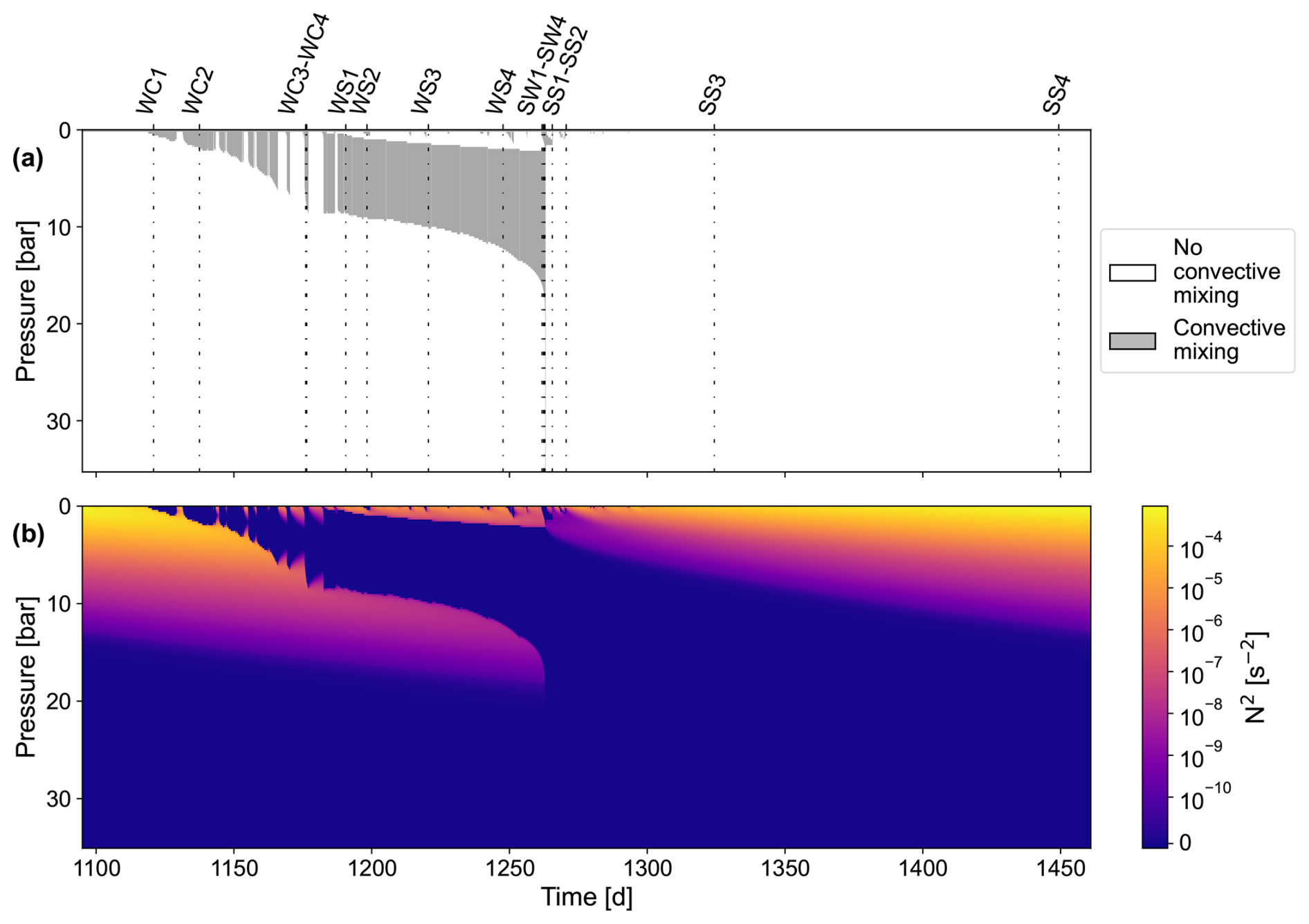
In autumn, cooling at the surface drives vertical convection due to instabilities in the water column (Fig. 5a) the same way as if thermobaricity was not included. The surface temperature is decreasing and the convective mixing extends vertically to the depth where the surface temperature is equal to the current temperature at this depth. This depth also decreases due to the colder surface temperatures (compare WC1-4 in Fig. 4a). The convective mixing is interrupted from short rewarming events but is always connected to the surface.

Figure 5 Convective mixing cells and stability of the fourth year of the simulation period. (a) shows the convective mixing cells and the points in time of the profiles shown in Fig. 4 are marked with dash-dotted lines. (b) depicts the corresponding Brunt-Väisälä frequency, calculated with Eq. (6).

Before reaching the bottom, temperatures at the surface fall below 3.98 °C and the stable inverse stratification terminates the circulation at the surface. Hence, the convection cell detaches from the surface (Fig. 5a). As it is permanently overlain by colder temperatures, no interruptions happen due to small rewarming events. These small rewarming events only induce additional small convective mixing cells at the surface, which are well separated from the deep circulation cell. Moreover, the deepening of the intersection of the temperature profile with the T_md line (compare WS1-3 in Fig. 4b) leads to a deepening of the upper end of the deep circulation cell. Finally the convection cell reaches the bottom (compare WS4 in Fig. 4b).

The convection in the deep water layers stops when the conditions for cabbeling disappear. This happens when surface temperatures rise above deep water temperatures (SW2 in Fig. 4c). The two convective mixing cells, the convective mixing at the surface and the deep water circulation, remain well separated. Afterwards, the deep convection stops and only the surface convective mixing cell remains in place (compare SW3 and SW4 in Fig. 4c), even though its depth decreases due to the change of T_md with depth. Below the T_md line, the warmer surface water is less dense than the colder deeper water, which limits the extent of the surface convective mixing cell.

After the surface temperature crosses 3.98 °C, only short intermittent cooling events can induce small surface convective mixing cells. In general, the water column becomes more stable and no convective mixing occurs until the end of the yearly cycle in September (compare SS1-4 in Fig. 4d).

3.3 Stability

The display of convection cells (Fig. 5a) is instructive for understanding vertical transport, but a quantitative approach to stability is desirable. Potential density is not applicable and in situ density is dominated by compression and hence does not provide much visual insight into stability either. However, we showed that the Brunt-Väisälä frequency can be calculated (Eq. 6, Fig. 5b). The convection cells can be identified as areas of stability 0 s⁻². They are sharply separated from areas of higher stability. Starting in October, the water column becomes unstable from the surface due to decreasing surface temperatures. Short rewarming events partly restabilize the unstable part at its upper end and diffusion does so at its lower end. After the detachment of the convection cell from the surface, a stable layer develops at the surface. Its lower end corresponds to the depth where the temperature profile intersects with the T_md line. The surface convective mixing cells originating from rewarming events can be identified by destabilized parts at the surface. After the deep convection ceases and the summer stratification sets in, the whole water column stabilizes due to the increasing surface temperatures and diffusion. Besides that, a marginally stabilized part remains close to the bottom for a long period. Towards the end of the summer stratification, it also becomes increasingly stable due to diffusion.

3.4 Simulation with potential density

To demonstrate the effect of thermobaricity, we conducted the exact same simulation as in Sect. 2.3 only substituting in situ density ρ_in-situ with potential density ρ_pot (i.e. neglecting thermobaric effects). We used the formulation of Tanaka et al. (2001) for ρ_pot as before. Cabbeling was included as an instantaneous destabilizing effect by setting the surface temperature equal to T_md in one time step for every transition of maximum ρ_pot, which is equivalent to the surface water temperature crossing 3.98 °C. Neglecting thermobaric effects change the size and the period of convective mixing cells and the water column stability fundamentally (Fig. 6). There is only one significant period of overturn after the summer stratification culminating in a brief complete overturn when surface temperatures cross T_md and go into winter stratification. Due to the missing change of T_md with depth there is no cabbeling during the winter stratification below the surface and no successive downwards circulation that would be further driven by thermobaricity. Another brief moment of deep overturn occurs when surface temperatures go into summer stratification, again crossing T_md. The small convective mixing cells at the surface still occur due to their origin from small rewarming events which are unaffected by the thermobaric effect.

Figure 6 Convective mixing cells and stability of the fourth year of the simulation period for the simulation using potential density ρ_pot instead of in situ density ρ_in-situ (compare Fig. 5). (a) shows the convective mixing cells and (b) depicts the corresponding Brunt-Väisälä frequency, calculated with Eq. (6).

3.5 Interannual variations

To check the effect of interannual variability for the simulation using in situ density, we added two more runs by elevating or lowering the surface temperature of the fourth year of the simulation period by 0.4 °C, respectively. Increasing the surface temperature leads to a weaker convective mixing during winter (Fig. 7b). A shorter and warmer cold period leads to less cold water at the surface. Hence, the intersection of the temperature profile with the T_md line deepens less and the deep water circulation is weakened. Depending on the strength of this change, convective mixing may not reach the bottom (compare Fig. 7b). Consequently, the temperature of the deep water is increased in the following winter and the convective mixing reaches the bottom earlier in that year.

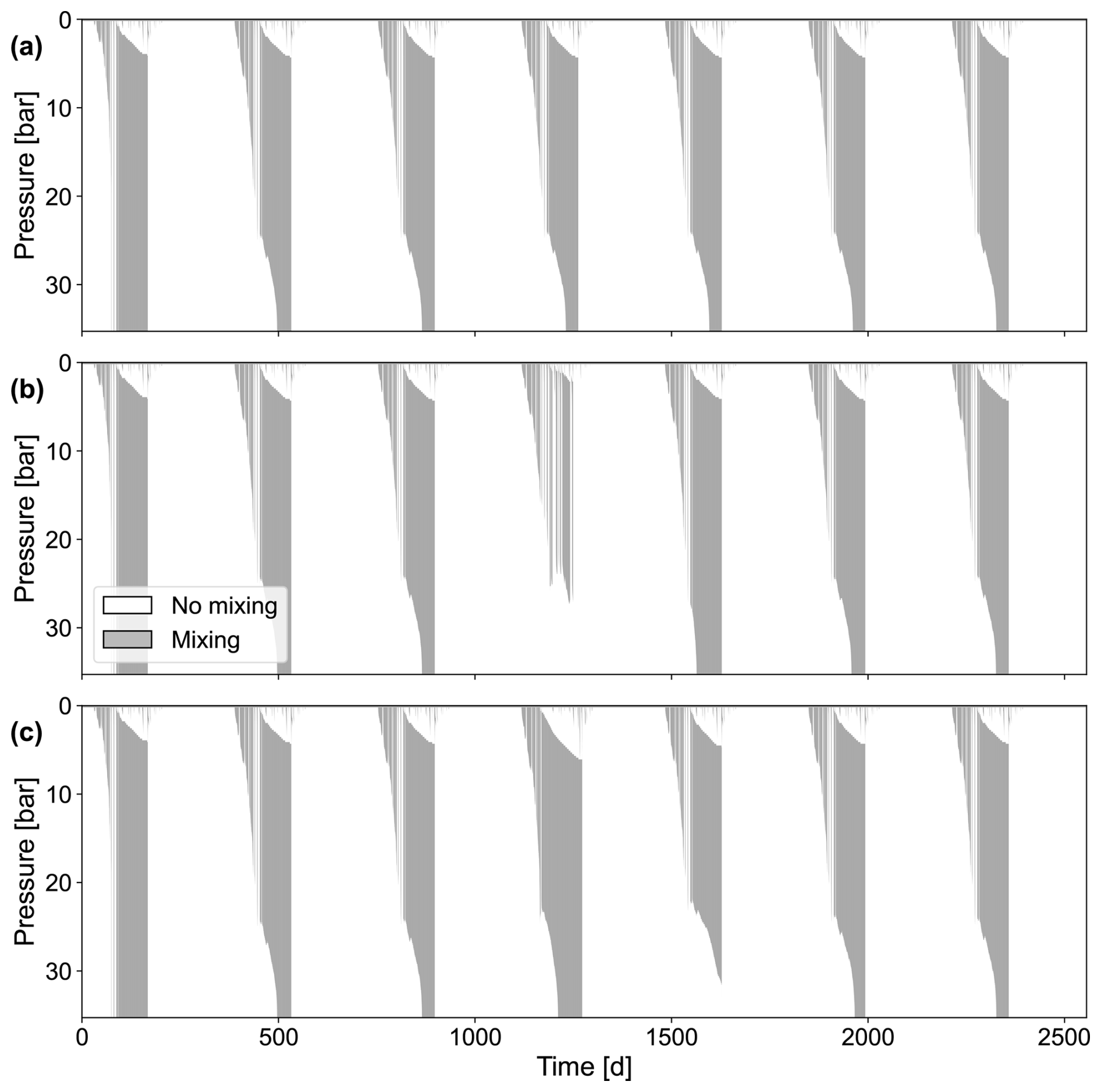
Figure 7 Mixing cells over the entire simulation period for three variants of surface temperature input. The surface temperature of the fourth year of the simulation period was (a) not modified, modified by (b) +0.4 °C, and (c) −0.4 °C.

In contrast, decreased winter temperatures enhance the convective mixing during winter (Fig. 7c). The colder temperatures and prolonged cold period leads to further deepening of the intersection of the temperature profile with T_md. Therefore, colder water is convectively mixed into the deep water and at the end of the deep circulation period colder isothermal deep water has been formed. As a result, the following year with the original surface temperature input has a less deep convective mixing cell since the colder deep water impedes deep convective mixing to the bottom (compare Fig. 7c).

In general, the variations in the surface temperature of successive years are in interplay with each other. They can either reinforce (e.g. a prior strong summer stratification and current cold winter period) or weaken (e.g. a prior weak summer stratification and current cold winter period) each other. Therefore, the model not only exhibits the different behavior of the convective mixing phases based on the variations in the forcing, the surface temperature, for the manipulated year, but also the dependency on the prior history. In general the stratification returns to normal after only a few years.

4 Discussion

With our numerical approach we intended to demonstrate (a) the effect of thermobaricity on a simple one dimensional system and (b) the proper representation of thermobaricity by stability considerations based on in situ density. Key features of this idealized thermobaric system were (1) diffusion induced cabbeling at the intersection of the temperature profile with the T_md line and its control of the deep water temperature by thermobaricity driven downwelling, (2) the period when surface water and deep water convection cells are separated, (3) the isothermal deep water, as well as (4) the alignment of the temperature profile with the T_md line in the upper water shortly after the winter stratification.

Despite the simplicity of our numerical approach, the key features (1)–(4) are remarkably clearly visible in the temperature profiles of Lake Shikotsu in 2005 (Fig. 1). The basic agreement of these features show that these thermobaric features in Lake Shikotsu (and other deep lakes with deep water temperatures below 3.98 °C) can be understood and basing stability considerations on in situ density can represent thermobaric effects.

We also tested the resilience of the thermobaric stratification against interannual variability. The simulations demonstrated the dependence of the deep water circulation on the surface temperature as driving force. They also showed that this type of circulation was quite resilient against disturbances and returned to the usual circulation pattern within two or three years. Of course, this is largely dependent on the many simplifications made in the model. Even though the general behavior is rather probable to stay similar, changes in the governing influences of the circulation would modify the systems responses so that a more comprehensive model would be needed for detailed investigations.

4.1 Previous lake models

To our knowledge only a few lake models have tackled the deep water circulation based on thermobaricity and all of them have focused on the wind induced displacement of cold surface water. Only Weiss et al. (1991) mentioned the possibility of mixing across T_md (vertical cabbeling) contributing to deep water circulation in just one sentence while apart from this also only focusing on wind induced downwelling in the very complex system of Lake Baikal. Walker and Watts (1995) created a three dimensional model to investigate the plume downwelling of displaced cold surface water based on thermobaric instabilities. Even though they mentioned the influence of turbulent diffusivity on creating instable conditions around the intersection of the temperature profile around T_md they did not expect the diffusivity to be responsible for deep water renewal on its own. Hence, they chose to focus on wind induced water displacement solely and only considered storm surge actions or internal waves as driving forces. Furthermore, Killworth et al. (1996) used a two dimensional and a one dimensional model to describe tracer measurements and the circulation in Lake Baikal. Here, their measurements indicated the newest water being at the bottom instead of isothermal deep water. This led them to focus on wind induced single plume downwelling of cold surface water as this is apparently more dominant than purely one dimensional vertical cabbeling induced mixing.

In contrast to the previous models, Farmer and Carmack (1981) applied a one dimensional mixing layer model to Babine Lake. They identified similar stratification phases as our model shows for Lake Shikotsu. However, Babine Lake experienced strong winds mixing the whole water column actively during the early inverse winter stratification before the ice cover set in. Nevertheless, during the mixing period the isothermal deep water successively cools down while the intersection of the temperature profile with the T_md line decreases, similar to our model. Farmer and Carmack (1981) associate this development to conditional instabilities induced by perturbations such as internal waves. But as our model shows mixing across T_md in form of vertical cabbeling may also contribute especially considering the similarities of the development of the temperature profiles. Additionally, Babine Lake demonstrates that for deeper lakes with ice cover the process of vertical cabbeling could be of more significance.

The more recent one dimensional model by Piccolroaz and Toffolon (2013) created for Lake Baikal also focuses on wind induced downwelling by using a resorting algorithm based on the initial surface water displacement by wind. Since they use Chen and Millero (1986) as equation of state and compare the densities based on the in situ temperature of the water parcels at the same pressure in their stability algorithm, we are convinced that their model in principle includes the vertical cabbeling as well. The presence of vertical cabbeling is simply not observable because of the much more dominant and overlying wind induced plume downwelling in Lake Baikal. Similarly, Wood et al. (2023) modified and applied this model to Crater Lake. They purely focus on the three dimensional thermobaricity driven deep downwelling as the influence of vertical cabbeling is also superimposed but presumably present.

4.2 Limitations and future development

A critical part of this parsimonious model is the exclusion of every external forcing except the surface temperature input. With the used input the heat balance of the lake with the atmosphere is considered. This also comes into play when the upper water column is mixed and the unstable water column is connected to the surface. In that case, the whole water column is set to the surface water temperature. This could lead to enormous heat fluxes in the model if the surface temperature input is not connected to measurements. By using measurements from Lake Shikotsu, we assumed the surface temperature values also represents the mixed epilimnion temperature well enough which ensures realistic temperatures for a mixed upper water column connected to the surface.

Nevertheless, more detailed influences of solar radiation and its penetration into the lake, also influenced by the turbidity, on the mixing of the epilimnion are ignored. Even though those influences are crucial for an comprehensive investigation of a lake, they do not influence the observed thermorbaric deep water circulation significantly due to the disconnection of the upper and lower mixing cells visible in the model as well as in Lake Shikotsu itself. Similarly, other aspects like wind, salinity, inflows, geothermal heating, and also the bathymetry itself would be needed for a comprehensive model. Those influences can induce or control different mixing or stratification patterns like e.g. submerged flow or salinity based stratification creating a double diffusive regime with geothermal heating. These processes could interfere or even totally overlay the observed one dimensional cabbeling induced themobaric deep circulation. In case of including salinity it would also become revelevant to consider conservative temperature instead of potential temperature (McDougall, 2003) which may need some adaption to be applied for lakes (e.g. Pawlowicz and Feistel, 2012, if TEOS-10 is used). Lake Shikotsu presents an good example of most of those influences being at least not dominant or even almost absent (Boehrer et al., 2009) which is why we decided to exclude them in the present model.

One external forcing that still plays an important role even in Lake Shikotsu is the wind. Measurements propose the absence of large wind induced downwelling as in for example Lake Baikal (Piccolroaz and Toffolon, 2013) due to the isothermal deep water (see Fig. 1b). However, the extend of the well mixed epilimnion is largely influenced by the amount of wind, especially during the inverse winter stratification. Hence, the wind also directly influences the depth at which the temperature profile intersects with the T_md line and therefore also the deep water temperature. To create a more realistic model it would be necessary to implement the wind to recreate the correct intersection depth and also check for potential, but seemingly rather weak if even present, wind forced downwelling as Piccolroaz and Toffolon (2013) do. The latter was explicitly excluded to ensure the visibility of the pure one dimensional effect of thermobaricity which is totally disconnected from wind in its basic characteristics and occurrence since cabbeling across the T_md line occurs even for the smallest diffusivity. To at least partly account for the wind enhanced mixing of the epilimnion and a corresponding deepening of the intersection of the temperature profile with the T_md line we chose a rather high background diffusivity.

The applied constant background diffusivity had a value of about $\mathrm{2.7}\times {\mathrm{10}}^{-\mathrm{4}}{\mathrm{m}}^{\mathrm{2}}{\mathrm{s}}^{-\mathrm{1}}$ to ensure a good visibility of the different phases of the one dimensional mixing without distancing too far from realistic values. More details on the chosen value and its influence on the model results are given in Appendix A. Basically, a different value of the constant diffusivity does not change the general behaviors of the present process but only determines how deep the cold/warm temperatures get in winter/summer. Nonetheless, a more realistic diffusivity should vary in space and time during the simulation to account for stratification in summer and winter and represent certain areas with higher turbulence like the well mixed surface layer. Those different areas would also influence the temperature gradient of the water column which could interfere with thermobaric controlled mixing, which is why we excluded spacial changes. Additionally, the diffusivity in our model is not time implicit. A time implicit diffusivity would ensure a more time realistic behavior of the model in general. Nevertheless, by exchanging parts of the water of each cell with the neighbouring layers to account for turbulent diffusion mixing across T_md is enabled, which is the only necessary characteristic of diffusion to enable one dimensional thermobaric circulation.

The mixing of unstable parts of the water column is also not time implicit. Currently, all unstable connected layers are equally mixed during one time step. This prevents realistic time scales and the correct development of the unstable water column parts, especially below the intersection of the temperature profile and the T_md line. Again, the change in this dynamic would change neither the occurrence nor the basic characteristic of the cabbeling induced thermobaric circulation. Still, if a time (and space) realistic circulation model is required time implicit formulations of diffusivity and active mixing as well as kinetic energy considerations are needed. This becomes even more important if more external influences, potentially varying in time and space, like inflows and geothermal heating are included.

In general, this one dimensional parsimonious model was meant to elucidate the purely one dimensional cabbeling induced thermobaric downwelling as well as emphasize the implementation of thermobaricity, for example by using in situ density for stability considerations. For a more comprehensive model including other important processes in lakes that interfere or even overlay the one dimensional thermobaric circulation other more elaborate models are needed and using in situ density can only be a first step. To generally incorporate a comprehensive thermodynamic concept and implement thermobaricity TEOS-10 would be a good way (see also Appendix B), which can be adapted to lakes. Additionally, other models, especially ocean models, start to or already include thermobaricity as well. Delft3D, being an ocean model that is also applicable to lakes, being one example of it. For future work it is planned to use Delft3D to simulate Lake Shikotsu in a more comprehensive way and analyze the system including the one dimensional thermobraic mixing.

5 Conclusions

In this paper, we presented an approach for implementing the effect of thermobaricity into a numerical model using in situ density instead of potential density. We created a simplified 1D model excluding any external forcing except the surface temperature. Below the surface layer, dynamics were exclusively driven by diffusion induced cabbeling around T_md and successive vertical convective mixing controlled by thermobaricity below, until stable density stratification was achieved. Moreover, we reduced the complexity to a minimum by omitting salinity, using horizontal homogeneity (one dimensional), a cylindrical bathymetry without shallow areas, and excluding any inflows or geothermal heating. Hence, the thermobaric effects could be displayed without competing influences. To remain in a realistic range and have a good chance to reproduce thermobaric effects, we used Lake Shikotsu as inspiration and used its maximum depth and surface temperature as input.

The model was able to conceptually characterize key features of the deep water circulation. It elucidated different phases of vertical mixing and presents the possible vertical and temporal extent of convection cells. Generally, the deep water circulation differed fundamentally from the conventional understanding (i.e. the mixing behavior when thermobaric effects are excluded) as well as from the wind forced downwelling including thermobaricity. During winter stratification, vertical cabbeling occurred at the intersection of the temperature profile with the T_md line due to diffusion which differs from the usual horizontal cabbeling at thermal bars. The vertical cabbeling then induced convective mixing below driven by thermobaricity which cools the deep water (compare Fig. 2). This convection cell was disconnected from the surface and extended into a depth where the temperature was equal to T_md at the intersection or to the bottom. The depth of the intersection of the temperature profile with the T_md line deepens with time due to ongoing cooling from above and associated cabbeling induced mixing of the deep water and therefore determines the resulting deep water temperature and the lower extent of the circulation cell. This circulation behavior was not only influenced by the current surface temperature but also by the previous history of deep water renewal events. For instance, colder winter enhanced deep water circulation but led to weaker convective mixing in subsequent years.

In summary, this simplified model exhibits the necessity and the feasibility of including thermobaricity in the simulation of deep water circulation and the existence of the one dimensional process of cabbeling induced thermobaric deep water circulation. This can be achieved by the implementation of in situ density (instead of potential density) for stability considerations. Despite the fact that this parsimonious approach could nicely reproduce the typical circulation features induced by thermobaricity, we are fully aware that a realistic representation of processes in Lake Shikotsu requires a proper lake model with complete forcing, time implicit formulations of diffusivity and mixing, and accurate bathymetry. Hence, the proper solution for future lake modeling is the appropriate inclusion of stability considerations based on in situ density into established lake models or to adapt comprehensive thermodynamic concepts including thermobaricity like TEOS-10. This feasible approach will provide new insights into deep water formation in thermobarically stratified lakes such as Lake Shikotsu and will improve the modeling of complex deep water renewal processes that are linked to thermobaricity as they occur in many large lakes.

Appendix A: Diffusivity analysis

To choose a suiting background turbulent diffusivity to be able to adequately visualize the observed cabbeling induced thermobaric circulation while staying in a reasonable range, we made several runs with different exchange fractions, listed in Table A1, for the chosen time step and layer size of 1 h and 2 m, respectively. We applied a homogeneous starting temperature profile of 5 °C with the lowest layer having 4 °C. By choosing this starting profile we ensured a stable water column over the whole simulation period of one year where we hold a constant surface temperature of also 5 °C so that only diffusion would play a role.

Table A1 Used exchange fractions, corresponding time steps and resulting diffusivities.

Figure A1 Temperature profiles for different applied exchange fractions at different time steps. The simulation setup is described in the text. The shown time steps for the corresponding exchange fractions are listed in Table A1. The gray dashed line indicates the depth at which the diffusivity values were evaluated.

Temperature profiles for the different applied exchange fractions for different time steps are given in Fig. A1. We chose the time steps to ensure an appropriate development of the temperature profile that is neither too close to the starting conditions nor too equally distributed since we still controlled the surface temperature. Those temperature profiles can then be used to calculate the diffusivity D using the following time step and Fick's second law

$$\begin{array}{}\text{(A1)}& {\displaystyle \frac{\partial T}{\partial t}}=D{\displaystyle \frac{{\partial }^{\mathrm{2}}T}{\partial z^{\mathrm{2}}}},\end{array}$$

here applied for the temperature T, with t and z being the time and depth, respectively. Using Eq. (A1) the diffusivity can be determined by

$$\begin{array}{}\text{(A2)}& D={\displaystyle \frac{\partial T}{\partial t}}{\left({\displaystyle \frac{{\partial }^{\mathrm{2}}T}{\partial z^{\mathrm{2}}}}\right)}^{-\mathrm{1}},\end{array}$$

with the discrete form of Eq. (A2) being

$$\begin{array}{}\text{(A3)}& D={\displaystyle \frac{T_{i,t+\mathrm{1}}-T_{i,t}}{\mathrm{\Delta }t}}{\left({\displaystyle \frac{T_{i+\mathrm{2},t}-\mathrm{2}{T}_{i+\mathrm{1},t}+T_{i,t}}{{\left(\mathrm{\Delta }z\right)}^{\mathrm{2}}}}\right)}^{-\mathrm{1}},\end{array}$$

with i representing the corresponding layer, Δz=2 m the layer thickness/layer distance, t the corresponding time step, and Δt=1 h the time step size. We evaluated the diffusivity values at a depth of 20 bar. Similarly to the time steps, we chose the depth to be neither too close to the surface boundary nor to the turning point of the temperature profile. The determined diffusivity values for the corresponding exchange fractions are listed in Table A1 and shown in Fig. A2. To describe the dependency of the diffusivity on the exchange fraction we propose the correlation

$$\begin{array}{}\text{(A4)}& D\left(\mathit{\nu }\right)={\displaystyle \frac{l\cdot \mathrm{0.5}\mathit{\nu }l}{t}},\end{array}$$

again with the layer size of l=2 m and time step size of t=1 h, which is also shown in Fig. A2.

Figure A2 Correlation of the diffusivity and the exchange fraction. The black crosses represent the diffusivities for the given exchange fractions and time steps (compare Table A1). The black line represents Eq. (A4).

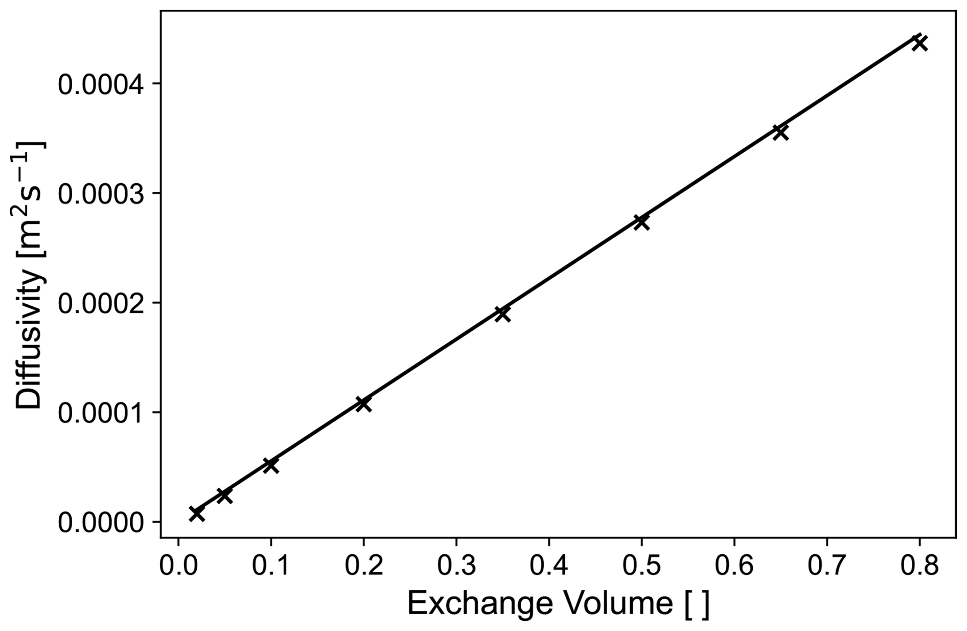
The proposed correlation seems to be a good estimation of the diffusivity values given the current model setup. For other time steps and different depths the diffusivity values can differ from this linear correlation but generally maintain their magnitude. However, the further the profiles develop from the starting profile and the better the selected depth is separated from the boundaries and the turning point the closer the calculated values get to the proposed correlation. Hence, we decided to use this correlation to estimate our background diffusivity which results in a value of $\mathrm{2.7}\times {\mathrm{10}}^{-\mathrm{4}}{\mathrm{m}}^{\mathrm{2}}{\mathrm{s}}^{-\mathrm{1}}$ for ν=0.5. This diffusivity value leads to a good visualization of the different mixing phases in the model while also being in the order of magnitude of previously used values in models for thermobaric circulation like Piccolroaz and Toffolon (2013) with $\mathrm{5}\times {\mathrm{10}}^{-\mathrm{5}}{\mathrm{m}}^{\mathrm{2}}{\mathrm{s}}^{-\mathrm{1}}$ for Lake Baikal and Wood et al. (2023) with about $\mathrm{1}\times {\mathrm{10}}^{-\mathrm{4}}{\mathrm{m}}^{\mathrm{2}}{\mathrm{s}}^{-\mathrm{1}}$ to $\mathrm{2}\times {\mathrm{10}}^{-\mathrm{3}}{\mathrm{m}}^{\mathrm{2}}{\mathrm{s}}^{-\mathrm{1}}$ (compare their Fig. 2) for Crater Lake.

To demonstrate that the general mixing behavior does not change for different diffusivity values, we present the simulation results for an exchange fraction of ν=0.05, which corresponds to a diffusivity of $\mathrm{2.4}\times {\mathrm{10}}^{-\mathrm{5}}{\mathrm{m}}^{\mathrm{2}}{\mathrm{s}}^{-\mathrm{1}}$ (which is the same order as in Piccolroaz and Toffolon, 2013), as an example (see Figs. A3 and A4). Depicted are the results for the 22nd year instead of the fourth year because the simulation needs more years until the initial conditions do not significantly effect the mixing patterns anymore because of the smaller diffusivity.

Figure A3 Similar to Fig. 4 but with an exchange fraction of ν=0.05 and the 22nd year shown.

Figure A4 Similar to Fig. 5 but with an exchange fraction of ν=0.05 and the 22nd year shown.

In general, the patterns of the mixing phases are similar to the simulation with an exchange fraction of ν=0.5. Due to the lower diffusion there is less deepening of the stratified surface layers in winter and summer. Accordingly, the intersection of the temperature profile with the T_md line is less deep in winter and the deep circulation cell starts closer to the surface. Hence, less cold water is circulating into the deep water and the bottom water is warmer compared to higher diffusivity values. This is why the deep circulation cell reaches the bottom only for a really short period. Because of the small threshold in the stability check the circulation does not necessarily reach the bottom every year for such low diffusivities since not enough heat is transported into the deep water during summer stratification. For larger diffusivity values the deep mixing would be enhanced correspondingly instead. However, the effect of diffusion inducing cabbeling at the intersection of the temperature profile with the T_md line and following deep circulation driven by thermobaricity still occurs for every chosen exchange fraction. Only the extend of the different mixing phases varies. Hence, we chose ν=0.5 for the best representation of all mixing phases while applying a diffusivity value of an adequate magnitude.

Appendix B: Using TEOS-10

Figure B1 Similar to Fig. 4 but using the density formulation of TEOS-10.

Figure B2 Similar to Fig. 5 but using the density formulation of TEOS-10.

To emphasize the fact that TEOS-10 (IOC et al., 2010) incorporates thermobaricity also in our simplified model we made the same simulation as in the main part but using the density formulation of TEOS-10 for the in situ density comparison in the stability algorithm and considered the conversion from potential temperature to conservative temperature. The latter, however, does practically not play a role in the mixing behavior, as it can be seen in the results (compare Figs. B1 and B2). The differences in the two temperatures are small in the temperature range of interest and since we excluded salinity essentially no production of potential temperature occurs during mixing (compare Fig. 2a in McDougall, 2003). For implementation of TEOS-10 we used McDougall and Barker (2011).

The results are similar to using Eq. (5) as simplified formulation for the in situ density for the simulation. Hence, generally using any appropriate in situ density to include thermobaricity may be a good option for adaptation of more extensive models already including certain thermodynamic considerations. However, TEOS-10 provides a powerful comprehensive thermodynamic framework taking care of conservative quantities especially if salinity is included. If desired, TEOS-10 can be adopted easily and applied to lakes (using e.g. Pawlowicz and Feistel, 2012, if salinity is included).