Enhanced Markov-type Categorical Prediction with geophysical soft constraints for hydrostratigraphic modeling

Accurately characterizing hydrostratigraphic structures is essential for reliable groundwater flow and transport modeling. Due to limited borehole coverage and geological complexity, uncertainty analysis plays a vital role in supporting robust hydrogeological modeling. Traditional geostatistical approaches such as Multiple-Point Statistics (MPS), offer flexibility in reproducing complex geological patterns and uncertainties, but they are computationally demanding, may struggle to maintain stratigraphic consistency, and can be difficult to apply in practice. Alternatively, the Markov-type Categorical Prediction (MCP) framework has a better computational efficiency and enforces stratigraphic ordering. However, its effectiveness is challenged in areas with sparse borehole data. To address this limitation, this study presents an enhanced MCP approach that incorporates airborne electromagnetic (AEM) geophysical data as soft probabilistic constraints on lithology occurrence. A tunable parameter controls the relative contribution of geophysical and geological information, allowing for flexible data integration within the simulation process. The approach is tested on both synthetic and real-world cases. Synthetic experiments of different scenarios demonstrate that incorporating geophysical constraints improves lithological prediction accuracy, particularly when combined with borehole data. In the field application from Egebjerg, Denmark, we demonstrate how a statistical relationship between lithology and resistivity can be derived by integrating SkyTEM data with borehole lithological logs and depth information. That relation is then combined with conditional probabilities from training images extracted from a 3D interpreted model, using the MCP framework. The results show that the integrated approach enhances the generations of complex geological features, such as buried valleys, especially in areas with limited direct observations. By embedding geophysical information into the MCP framework, the method combines the spatial consistency and stratigraphic ordering of MCP with the extensive coverage and subsurface sensitivity of geophysical data. This integration overcomes a key limitation of MCP and enables more reliable simulations in regions where direct subsurface observations are limited, providing a practical and adaptable tool for improving geological modeling in groundwater studies.

1 Introduction

In hydrogeological modeling, uncertainty analysis is essential to account for the incomplete knowledge of subsurface conditions and to support robust decision-making in water resource management, contamination risk assessment, and infrastructure planning (e.g. Feyen and Caers, 2006; Hermans et al., 2023). Subsurface environments are inherently heterogeneous and data available for modeling, such as borehole logs, are typically sparse and unevenly distributed in space. Without explicitly quantifying uncertainty, predictions based on deterministic models risk to misrepresent hydrogeological processes and may lead to ineffective or even damaging management strategies (Koch et al., 2014; Vilhelmsen et al., 2019). This is particularly true when deterministic models are used as the basis for groundwater flow and solute transport simulations, where small inaccuracies in hydrostratigraphic structure can lead to significant deviations in predicted flow paths, travel times, and contaminant breakthrough curves (Dai et al., 2017; Zuo et al., 2023; Song et al., 2019). By incorporating uncertainty into the simulation of geological heterogeneity, geostatistical approaches provide not only plausible geological scenarios but also essential input for ensemble-based hydrogeological forecasting, which is one type of probabilistic approach that relies on multiple realizations to assess model uncertainty (e.g. Enemark et al., 2024; Hermans et al., 2015).

In constructing geostatistical models, borehole data are the most commonly used conditioning data because they provide direct observations of subsurface lithology (Boyd et al., 2019; Madsen et al., 2021). However, the cost, time, and logistical constraints of drilling often result in insufficient borehole coverage, especially at greater depths or in poorly accessible regions (Bongajum et al., 2013; Madsen et al., 2022). In contrast, geophysical exploration methods, such as electrical resistivity tomography (ERT) or airborne transient electromagnetic (AEM) surveys, offer a cost-effective way to obtain relatively high-density spatial coverage (e.g. Maurya et al., 2023; Prikhodko et al., 2024). Although geophysical data do not directly measure lithology, they provide property contrasts (e.g., in resistivity) that, after inversion and interpretation, can be statistically linked to hydrofacies distributions (Michel et al., 2020; Pirot et al., 2017).

Within geostatistical modeling, constructing a reliable hydrostratigraphic model typically requires integrating multiple sources of information, including hard data (e.g. borehole observations), probabilistic constraints (e.g. resistivity models derived from inverted airborne geophysical measurements), and prior geological knowledge about spatial variability and continuity, typically expressed through the form of a covariance model or training image (TI) (He et al., 2014; Høyer et al., 2017; Barfod et al., 2018). Each of these sources contributes complementary information: boreholes offer detailed but localized information, geophysical data provide indirect insights into large-scale hydrostratigraphic architecture, and TIs capture prior geological knowledge and spatial continuity. Combining them leads to more robust and geologically realistic models (Barfod et al., 2018; Jha et al., 2014). However, this integration is not straightforward, as it requires a quantitative understanding of the relationships between different data types. Without careful treatment, combining data of varying resolution, quality, and interpretability may lead to overinterpretation or underutilization of valuable information (Levy et al., 2024).

Multiple-Point Statistics (MPS) has become a widely used geostatistical method in hydrostratigraphical modelling. MPS uses Training Images (TIs) to quantify the spatial variability and reproduce complex geological patterns that cannot be captured by traditional two-point geostatistics (Guardiano and Srivastava, 1993; Mariethoz and Caers, 2014). In recent years, several studies have explored introducing probabilistic spatial constraints, including geophysical models, into MPS frameworks. For example, Barfod et al. (2018) demonstrated that conditioning MPS simulations with airborne electromagnetic data significantly improved the delineation of buried valleys in Denmark. Madsen et al. (2021) proposed treating uncertain geological interpretations as probabilistic constraints, comparing MPS and Gaussian simulation methods, and showed that MPS produced more geologically plausible and connected realizations. Hermans et al. (2015) developed a full MPS-based inversion framework that used ERT data both to falsify prior geological scenarios and to locally constrain groundwater simulations, showing the strength of MPS in quantifying uncertainty and integrating multiple data types. Lochbühler et al. (2014) demonstrated that tomographic images can be used to condition multiple-point statistics facies simulations, thereby improving the structural consistency of simulated geological models. Despite these advances, several challenges remain, MPS methods are computationally expensive and highly sensitive to TIs that are geologically realistic and representative of the entire site (He et al., 2014; Levy et al., 2024). A TI of limited extent can lead to biased simulations that misrepresent key structural features. Most existing MPS approaches, such as Direct Sampling (Meerschman et al., 2013), still treat soft or geophysical data in a heuristic manner, through secondary TIs rather than probabilistic conditioning (e.g., Lochbühler et al., 2014), so they cannot explicitly address non-stationarity within a probabilistic framework. Many existing implementations of geostatistical simulation, such as MPS-based methods, cannot enforce explicit geological transition rules, for instance those arising from successive sedimentary deposition processes, which means that they may fail to represent stratigraphic relationships accurately, particularly those relevant to spatial shifts in facies proportions or variations in layer thickness. Both limitations are critical when simulating subsurface structures for groundwater flow and transport modeling (Cordua et al., 2016; Kim et al., 2017).

A recently applied geostatistical approach by Benoit et al. (2018), known as Markov-type Categorical Prediction (MCP), provides an alternative framework to traditional MPS for simulating categorical geological units. MCP uses bivariate transition probabilities derived from a TI. One of the key advantages of MCP is that it reduces the dependence on high-quality or highly repetitive TIs, which can be a limiting factor in some MPS implementations (Allard et al., 2011). When key features in the TI are sparse, irregular, or unique, MPS may struggle to reproduce them consistently, potentially leading to artificial discontinuities or oversimplified realizations (Barfod et al., 2018). By contrast, MCP operates on a different principle. Rather than trying to reproduce entire patterns from the TI, MCP uses pairwise transition probabilities between units to capture the likelihood of one unit being adjacent to another (Benoit et al., 2018). This approach allows MCP to extract essential geological information in a non-stationary fashion without needing a complete TI. Furthermore, MCP remains computationally efficient, even when simulating models with a large number of lithological categories because it avoids high-order pattern scanning or search-tree construction. One of MCP's strengths is its ability to strictly respect geological rules when certain transitions between units are geologically impossible. For example, if a specific lithological unit is never observed directly above another in the training data, MCP ensures that this configuration will not appear in the simulated model based on zero bivariate probability of these two units (Benoit et al., 2018). Yet, previous applications of the MCP framework have relied almost exclusively on hard conditioning data, such as borehole lithology. In settings where such data are sparse, the method often defaults to random simulation, which can result in geologically unrealistic outputs (Benoit et al., 2018). However, MCP offers greater transparency and flexibility in conditioning, making it well suited for the integration of soft information derived from geophysical inversion models, as we have demonstrated before on 2D synthetic data in Guo et al. (2024). The present work extends the MCP framework by incorporating geophysical soft constraints into the simulation process, weighted through the principle of permanence of ratios (Isunza Manrique et al., 2023). Applied to a real-world 3D geological setting, this integration enables a comprehensive quantitative evaluation of uncertainty reduction and improved geological realism, particularly in areas that are poorly constrained by hard data.

This paper is organized as follows. Section 2 introduces the principles of the Markov-type Categorical Prediction (MCP) framework and outlines its extension for integrating geophysical soft constraints. Section 3 presents the results in two parts. In Sect. 3.1, a synthetic test case is developed, where a true lithological model with multiple layers is defined and conductivity values are assigned using a Gaussian random field. Airborne electromagnetic data are simulated via 1D forward modeling and subsequently inverted using a 1D inversion scheme. The resulting inverted conductivity model is then statistically linked to the true lithology to derive a stochastic relationship, which is incorporated into the MCP framework as an additional constraint. Section 3.2 applies the proposed approach to a real-case study in Egebjerg, Denmark. Bivariate transition probabilities are computed from multiple 2D transects extracted from a 3D interpreted geological model and merged using the Extended Logistic Opinion Pool (ELOP) method to ensure directional consistency. The resulting representative transition probabilities serve as priors for MCP simulations along all transects, enabling the construction of a coherent 3D lithological model. Two representative transects, located in areas with shallow boreholes, are selected for detailed analysis to evaluate the added value of geophysical constraints. Borehole lithology, borehole depth information, and inverted resistivity from AEM data are statistically linked, and this relationship is combined with MCP probabilities through a tunable integration parameter. Finally, constrained MCP simulations are performed to generate multiple lithological realizations, allowing uncertainty quantification and assessment of geophysical constraints. Section 4 discusses the key methodological implications and insights derived from these extended MCP framework applications.

2 Methodology

2.1 Markov-Type Categorical Prediction

Markov-Type Categorical Prediction (MCP) is a probabilistic approach to generate categorical geological models that effectively maintains spatial relationships in a computationally efficient fashion. Within the MCP framework, it is assumed that the influence of neighboring categories on the target location can be captured through individual transition probabilities from the target to each neighbor, with independent interactions among the neighbors themselves. This conditional independence assumption simplifies computations by considering that the categorical states of neighboring points are independent once the category at the target location is known. Although a simplification, it has been shown to produce accurate and unbiased predictions in some geostatistical applications (Benoit et al., 2018).

Given a set of known categories $i_{\mathrm{1}},i_{\mathrm{2}},\mathrm{\dots },i_n$ at neighborhood locations $x_{\mathrm{1}},x_{\mathrm{2}},\mathrm{\dots },x_n$, the conditional probability of category i₀ at an unsampled location x₀ is calculated as: (Allard et al., 2011):

$$\begin{array}{}\text{(1)}& P_{i_{\mathrm{0}}|i_{\mathrm{1}},\mathrm{\dots },i_n}^{\mathrm{MCP}}={\displaystyle \frac{p_{i_{\mathrm{0}}}\prod _{k=\mathrm{1}}^n{p}_{i_k|i_{\mathrm{0}}}}{\sum _{i_{\mathrm{0}}=\mathrm{1}}^I{p}_{i_{\mathrm{0}}}\prod _{k=\mathrm{1}}^n{p}_{i_k|i_{\mathrm{0}}}}}={\displaystyle \frac{p_{i_{\mathrm{0}}}^{\mathrm{1}-n}\prod _{k=\mathrm{1}}^n{p}_{i_k,i_{\mathrm{0}}}}{\sum _{i_{\mathrm{0}}=\mathrm{1}}^I{p}_{i_{\mathrm{0}}}^{\mathrm{1}-n}\prod _{k=\mathrm{1}}^n{p}_{i_k,i_{\mathrm{0}}}}},\end{array}$$

where i₀ is the category being predicted, i_k are the observed categories in the neighborhood of x₀, and I is the total number of possible categories (e.g., lithological units). Given a set of observed categories $\mathit{\{}{i}_{\mathrm{1}},i_{\mathrm{2}},\mathrm{\dots },i_n\mathit{\}}$ at neighborhood locations $\mathit{\{}{x}_{\mathrm{1}},x_{\mathrm{2}},\mathrm{\dots },x_n\mathit{\}}$, the bivariate probabilities $p_{i_k,i_{\mathrm{0}}}$ quantify the likelihood of co-existence between two categorical states. The marginal probability $p_{i_{\mathrm{0}}}$ represents the prior likelihood of category i₀; in this study, it is defined as the mean proportion of each lithology observed in the training image.

A key step in MCP implementation involves defining the spatial range of the search neighborhood (x_n) around each estimation point. This range is a user-defined parameter that can be tuned to balance spatial continuity and computational cost. Following Benoit et al. (2018), we adopted an octant-based search strategy with at least one neighbor per octant, resulting in up to eight conditioning data per location.

The MCP approach requires a representative TI, from which the bivariate probabilities P(i_k,i₀) are derived and used in Eq. (1). These probabilities describe the likelihood of observing a pair of categories (i,j) separated by a specific lag h, and they are computed directly from the TI. To compute the bivariate probability between categories i at location x and category j at location x+h, we use the cross-indicator covariance:

$$\begin{array}{}\text{(2)}& P\left(I\right(\mathit{x}),J(\mathit{x}+\mathit{h}\left)\right)=E\left[I\right(\mathit{x}\left)J\right(\mathit{x}+\mathit{h}\left)\right],\end{array}$$

where I(x) and J(x+h) are binary indicator functions defined as I(x)=1 if the category at location x is i, and 0 otherwise. Similarly, J(x+h) takes value one if j is observed at point x+h. The expectation is taken over all valid pairs of grid nodes separated by vector h in the TI. The estimation of the probabilities is efficiently handled by a method by Marcotte (1996), which relies on the fast Fourier transform to calculate correlations accross multiple spatial lags.

The method is implemented using a sequential simulation framework, where categorical values are assigned iteratively based on the computed conditional probabilities using Eq. (1). The simulation begins with a blank grid, except for available hard data (e.g., borehole observations) . At each iteration, a location x_i is selected following a random path. If sufficient neighboring points are found within the defined octant-based search range, the conditional probability for each possible category at that location is computed using the bivariate transition probabilities. If no neighbors are available, the simulation falls back to using marginal probabilities alone derived from the training image. Once the conditional probability distribution is determined, a category is sampled using random sampling, and the simulated value is assigned to the location. The newly simulated point then is added to the conditioning neighborhood and contributes to the estimation of subsequent nearby nodes. This process continues until the entire simulation domain is completed, resulting in a single categorical realization. The procedure can be repeated multiple times to generate an ensemble of realizations, which can then be used for uncertainty analysis.

A distinctive feature of MCP is its zero-forcing property, which guarantees that if a bivariate probability between two categories is zero, the corresponding category transition over a considered distance is completely restricted in the generated realizations (Allard et al., 2011). This property makes MCP particularly suitable for modeling stratigraphic sequences where ordering constraints must be preserved (Benoit et al., 2018). However, in regions with limited conditioning data, MCP may revert to using marginal probabilities when neighborhood information is insufficient, which can lead to the occurrence of geologically incompatible transitions. To address this, a post-processing correction procedure is introduced in Sect. 2.4 to enforce geological consistency in the final simulations.

2.2 Integration of geophysical data

Geophysical data can provide additional constraints to geostatistical simulations by linking lithological categories with physical properties (Hermans et al., 2015). In the present study, a stochastic resistivity-lithology relationship is established by deriving conditional probabilities from inverted resistivity models. Unlike most previous MPS-based approaches, which typically overlook the spatial degradation of geophysical resolution, our method explicitly incorporates both the smoothing effects of regularized inversion and the loss of resolution with depth into the probabilistic framework (Hermans and Irving, 2017; Hermans et al., 2015; Barfod et al., 2018; Deleersnyder et al., 2023). These probabilities represent the likelihood of observing specific lithological classes given the resistivity values at corresponding locations.

To integrate this information with the categorical constraints from the MCP framework, the permanence-of-ratios principle is applied. This principle assumes that the relative influence of different data sources can be preserved through a ratio-based formulation. The intermediate quantities used in this formulation are defined as follows (Journel, 2002; Isunza Manrique et al., 2023):

$$\begin{array}{}\text{(3)}& \begin{array}{rl}& a={\displaystyle \frac{\mathrm{1}-P\left(A\right)}{P\left(A\right)}},b={\displaystyle \frac{\mathrm{1}-P\left(A\right|B)}{P\left(A\right|B)}},\\ & c={\displaystyle \frac{\mathrm{1}-P\left(A\right|C)}{P\left(A\right|C)}},x={\displaystyle \frac{\mathrm{1}-P\left(A\right|B,C)}{P\left(A\right|B,C)}},\end{array}\end{array}$$

where P(A) represents the marginal probability of lithology A, P(A|B) is the conditional probability of lithology A based on MCP constraints B, and P(A|C) reflects the conditional probability of lithology A given the geophysical data C, which is derived from inverted resistivity models through lithology–resistivity calibration. For the synthetic case, this relationship is established using the complete training image, whereas for the real-field application, it is calibrated using borehole lithological data. The final joint probability $P\left(A\right|B,C)$, conditioned on both sources, is obtained using the following proportionality:

$$\begin{array}{}\text{(4)}& {\displaystyle \frac{x}{b}}={\left({\displaystyle \frac{c}{a}}\right)}^{\mathit{\tau }}.\end{array}$$

Solving for $P\left(A\right|B,C)$ yields:

$$\begin{array}{}\text{(5)}& P\left(A\right|B,C)={\displaystyle \frac{a^{\mathit{\tau }}}{a^{\mathit{\tau }}+b\cdot c^{\mathit{\tau }}}}.\end{array}$$

Here, the exponent parameter τ controls how strongly the model emphasizes differences between the components a and c. As τ increases, the contrast between these terms becomes more pronounced, allowing the model to more clearly favor the source (prior or geophysical) with the stronger signal. This enables flexible adjustment of the relative influence of geophysical data, depending on the level of confidence in its relationship to the target property.

During the sequential MCP simulation, for each unsimulated node, the conditional probability P(A|B) is first computed using Eq. (1), based on the bivariate transition probabilities inferred from neighboring lithological categories. This MCP-based probability is then combined with the geophysically derived conditional probability P(A|C) through the permanence-of-ratios formulation (Eq. 5), yielding the joint probability $P\left(A\right|B,C)$. The resulting distribution $P\left(A\right|B,C)$ is subsequently used as the sampling distribution to assign the lithofacies at that node.

Once the joint probabilities are computed for all categories and locations, multiple realizations of the subsurface lithology are generated using the sequential simulation framework of the MCP algorithm. The integration of resistivity based probabilistic information serves to guide the categorical simulation toward geologically plausible outcomes that also honor the spatial patterns suggested by the geophysical data.

To better evaluate the uncertainty of added geophysical constraints in our MCP simulations, we computed entropy maps which measure the diversity of predicted lithology categories at each location based on the Shannon entropy (Pirot et al., 2022) across realizations.

The entropy at each grid location (i,j) was calculated using Shannon's entropy to quantify the uncertainty in lithological prediction:

$$\begin{array}{}\text{(6)}& H\left(Z_{i,j}\right)=-\sum _{l=\mathrm{1}}^L{p}_l(i,j)\log \left(p_l(i,j)+\mathit{\epsilon }\right)\end{array}$$

where H(Z_i,j) denotes the entropy at location (i,j), L is the total number of lithology classes, p_l(i,j) is the empirical probability of class l at location (i,j) based on the realizations, and ε is a small constant added to prevent numerical issues when $p_l(i,j)=\mathrm{0}$.

2.3 General Workflow

The general workflow of the MCP framework incorporating geophysical data constraints is as follows (Fig. 1). Case-specific workflows for the synthetic and real-field applications are presented later to highlight differences in data sources and processing steps.

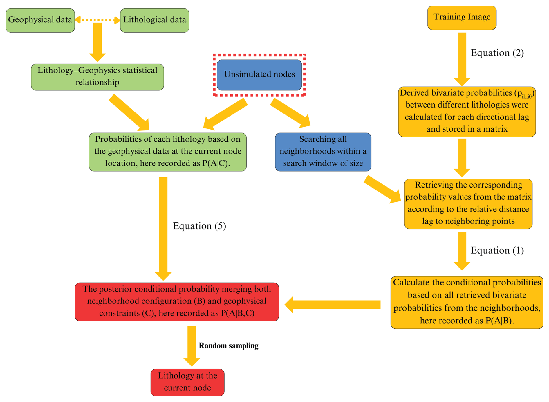
Figure 1 Workflow for the MCP framework constraint with geophysical data. Blue boxes represent the operational steps at the current unsimulated node. Green boxes represent the processing of geophysical data and its statistical calibration with lithology. Yellow boxes illustrate the extraction and integration of prior geological information from TIs for MCP calculations. Red boxes indicate the final probabilistic merging and categorical simulation steps.

2.4 Post-processing

Although the MCP framework has the property to preserve stratigraphic ordering through directional transition probabilities, violations may still occur in practice. Such inconsistencies can arise during the early stages of simulation, when no neighboring points are yet available and the algorithm must rely solely on marginal probabilities. Besides, in scenarios where borehole (hard) data are sparse, larger weight is assigned to the geophysical soft constraints, thus these may inadvertently steer the simulation toward geologically unrealistic category choices. To ensure geological plausibility and spatial continuity in the final realizations, two correction rules are implemented to identify and resimulate inconsistent cells.

1. Neighborhood consistency check: Each simulated cell is compared with its 24 current neighbors within a 5×5 window. If fewer than 9 neighbors had the same lithological category as the center cell, it is marked as inconsistent and is resimulated again.

2. Vertical consistency check: This rule enforces stratigraphic order by checking the relative of lithological units. For each cell, up to 6 cells directly above it are evaluated. If at least one of those upper neighbors represented older lithologies (had a higher category number), the current cell is flagged as violating geological logic and marked for resimulation.

Once inconsistent cells are identified through the rules above, they were removed and resimulated again. Then, all successfully simulated values from previous iterations are retained and treated as hard conditioning data in the sequential simulation approach. This means that as the correction process progresses, the MCP framework becomes increasingly guided by a growing set of accepted values, which helps to stabilize the simulation and maintain spatial consistency. If no inconsistent cells are identified in a given iteration, the simulation is considered consistent and the process is terminated. Otherwise, the procedure is repeated until either the number of incorrect cells remains unchanged for three consecutive iterations or a maximum of 40 iterations is reached. At that point, the final simulation result is accepted.

3 Results

3.1 Synthetic case

To validate the integration of geophysical constraints into the MCP framework, a synthetic case study was designed. This experiment aimed to assess the ability of the integrated approach to accurately reproduce lithological structures under different data availability conditions. By integrating geophysical data into the MCP simulation process, we evaluate the method's capacity to reduce uncertainty and improve geological realism prior to real-world applications.

The complete workflow of the synthetic case is summarized below and visually illustrated in Fig. 2:

1. A manually synthetic three-layer lithological model is constructed on a 2D 80×50 grid. The training image (TI) used in the synthetic case corresponds to this simplified three-layer model, containing three categorical facies.

2. A Gaussian random field is used to generate spatially correlated conductivity values within each lithology, based on the mean and standard deviation values in Table 1.

3. Synthetic AEM data are generated from the conductivity model from Step 2 with the 1D TDEM forward modelling routine available in the SimPEG package (Heagy et al., 2020).

4. The synthetic AEM data are then inverted using a 1D deterministic inversion. The inversion employed a smoothness-constrained regularization scheme, generating an inverted conductivity model.

5. The bivariate probabilities are derived from the synthetic training image, which are then used to calculate the conditional probabilities for the MCP function as in Eq. (1). In the constrained scenarios, a single borehole located X=8 m is introduced as hard conditioning data.

6. A stochastic resistivity–lithology relationship is derived by linking the inverted conductivity values to the true lithology classes at each grid cell (Hermans and Irving, 2017). This represents an idealized setting in which lithology and inverted resistivity data are fully co-located, and the resulting relationship is integrated into the MCP framework following the approach outlined in Sect. 2.2.

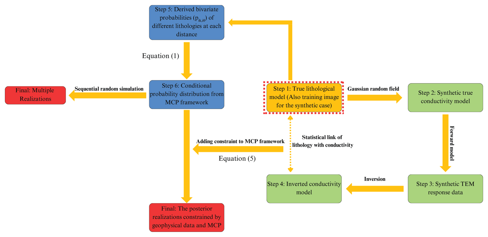
Figure 2 Workflow for the synthetic case. The yellow box represents the true synthetic lithological model, while green boxes denote the generation and inversion of geophysical data to derive conductivity constraints. Blue boxes represent the sequential steps of the MCP framework, including the extraction of bivariate probabilities from the training image. The red boxes indicate the final simulation outcomes, providing a direct comparison between the baseline realizations using pure MCP and the posterior realizations generated from the extended MCP framework with integrated geophysical constraints.

3.1.1 Model Setup

The synthetic lithological model consists of three distinct lithological units, as shown in Fig. 3 (left). The associated electrical conductivity model (right) is generated by assigning values to each lithology located at each grid cell using a Gaussian random distribution. This process corresponds to an isotropic Gaussian covariance model, with the correlation length controlled by the standard deviation of the filter. The specific parameters used for each lithology, including mean, standard deviation, and correlation length, are summarized in Table 1.

Table 1 Conductivity parameters assigned to each lithological layer in the synthetic model.

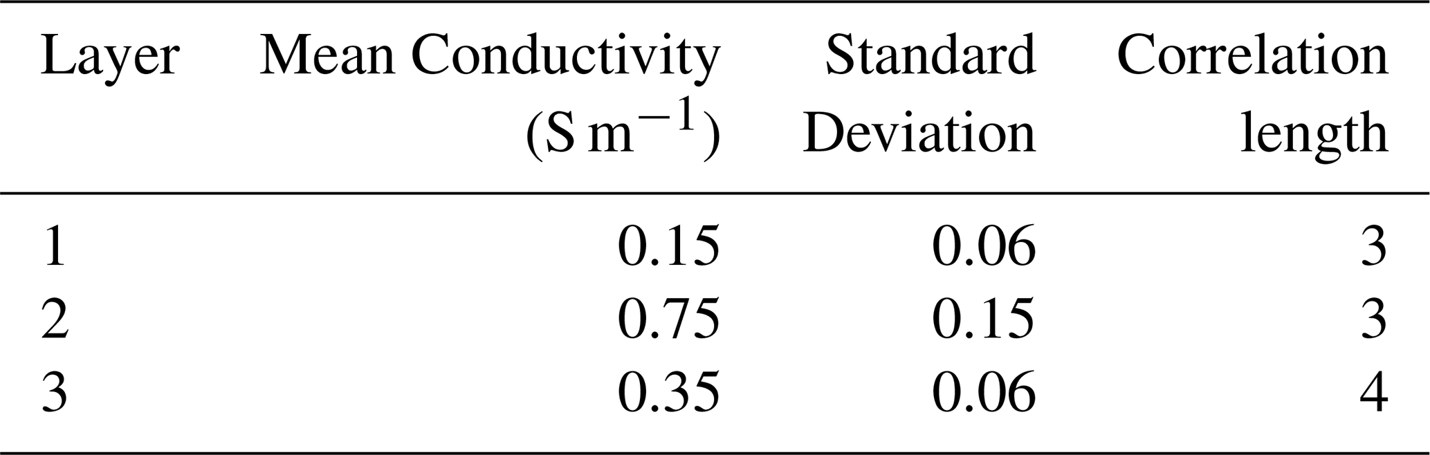
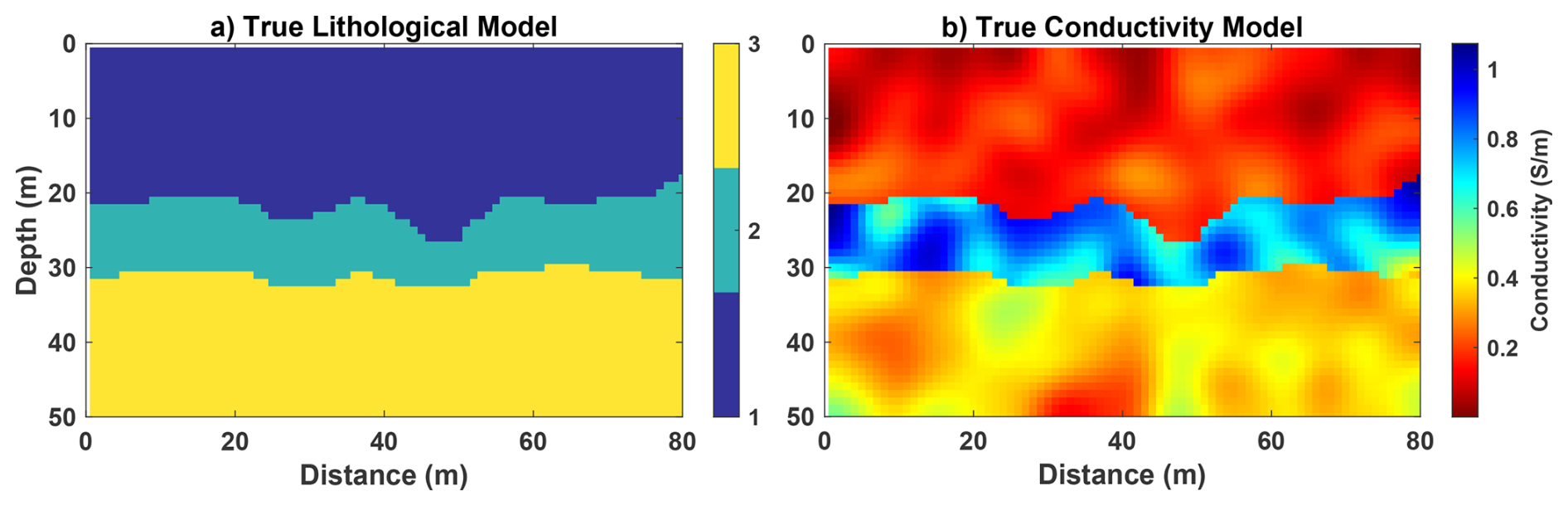
Figure 3 (a) Synthetic lithological model. (b) Synthetic conductivity distribution generated from the Gaussian random field.

3.1.2 Geophysical Forward and Inversion Modelling

The TEM responses were generated using a 1D layered forward modelling routine based on the synthetic lithological model. A circular loop transmitter positioned at 20 m height with a step-off waveform and was simulated using 21 logarithmically spaced time channels between 10⁻⁵ and 10⁻² s. A multiplicative Gaussian noise level of 2 % was added to the synthetic data to simulate realistic measurement noise.

For the inversion, the subsurface was discretized using 30 logarithmically spaced layers with thicknesses ranging from 0.5 to 5 m, reflecting the decreasing vertical resolution characteristic of TEM systems. The model parameters were defined in log-conductivity space to ensure positivity.

The data misfit was formulated as a weighted L₂ norm,

$$\begin{array}{}\text{(7)}& {\mathit{\varphi }}_d\left(\mathit{m}\right)={∥\mathbf{W}\left({\mathit{d}}_{\mathrm{obs}}-{\mathit{d}}_{\mathrm{pred}}\left(\mathit{m}\right)\right)∥}_{\mathrm{2}}^{\mathrm{2}},\end{array}$$

where m denotes the vector of log-conductivity model parameters, d_obs and d_pred(m) are the observed and predicted TEM responses, and $\mathbf{W}=\mathrm{diag}(\mathrm{1}/\mathit{\sigma })$ is the data weighting matrix with $\mathit{\sigma }=\mathrm{0.02}\left|{\mathit{d}}_{\mathrm{obs}}\right|$.

To stabilize the inversion, the objective function was augmented with a Tikhonov regularization term (Constable et al., 1987), combining zero-order and first-order vertical smoothness constraints:

$$\begin{array}{}\text{(8)}& {\mathit{\varphi }}_m\left(\mathit{m}\right)={\mathit{\alpha }}_s\Vert \mathit{m}{\Vert }_{\mathrm{2}}^{\mathrm{2}}+{\mathit{\alpha }}_x\Vert \mathrm{\nabla }\mathit{m}{\Vert }_{\mathrm{2}}^{\mathrm{2}},\end{array}$$

with α_s=0.01 and α_x=1.0. The trade-off parameter λ, which balances data fit and smoothness, was estimated from the dominant eigenvalue of the approximate Hessian to ensure consistent scaling.

The inverse problem is solved by minimizing the objective function:

$$\begin{array}{}\text{(9)}& \mathit{\varphi }\left(\mathit{m}\right)={\mathit{\varphi }}_d\left(\mathit{m}\right)+\mathit{\lambda }{\mathit{\varphi }}_m\left(\mathit{m}\right),\end{array}$$

where the optimization is performed using a projected Gauss–Newton Conjugate-Gradient (GNCG) algorithm. The resulting recovered and true models are shown in Fig. 4.

These inverted profiles are then statistically linked to the true lithology by evaluating the joint occurrence frequencies between conductivity and lithology classes across the grid. From this, we compute the conditional probability of lithology given conductivity, denoted as P(A|C), which is used as the soft geophysical constraint in the MCP framework:

$$\begin{array}{}\text{(10)}& P\left(A\right|C)={\displaystyle \frac{P(A,C)}{P\left(C\right)}},\end{array}$$

where P(A,C) is the joint probability distribution obtained from co-occurrence counts in the synthetic grid, and P(C) is the marginal probability of conductivity.

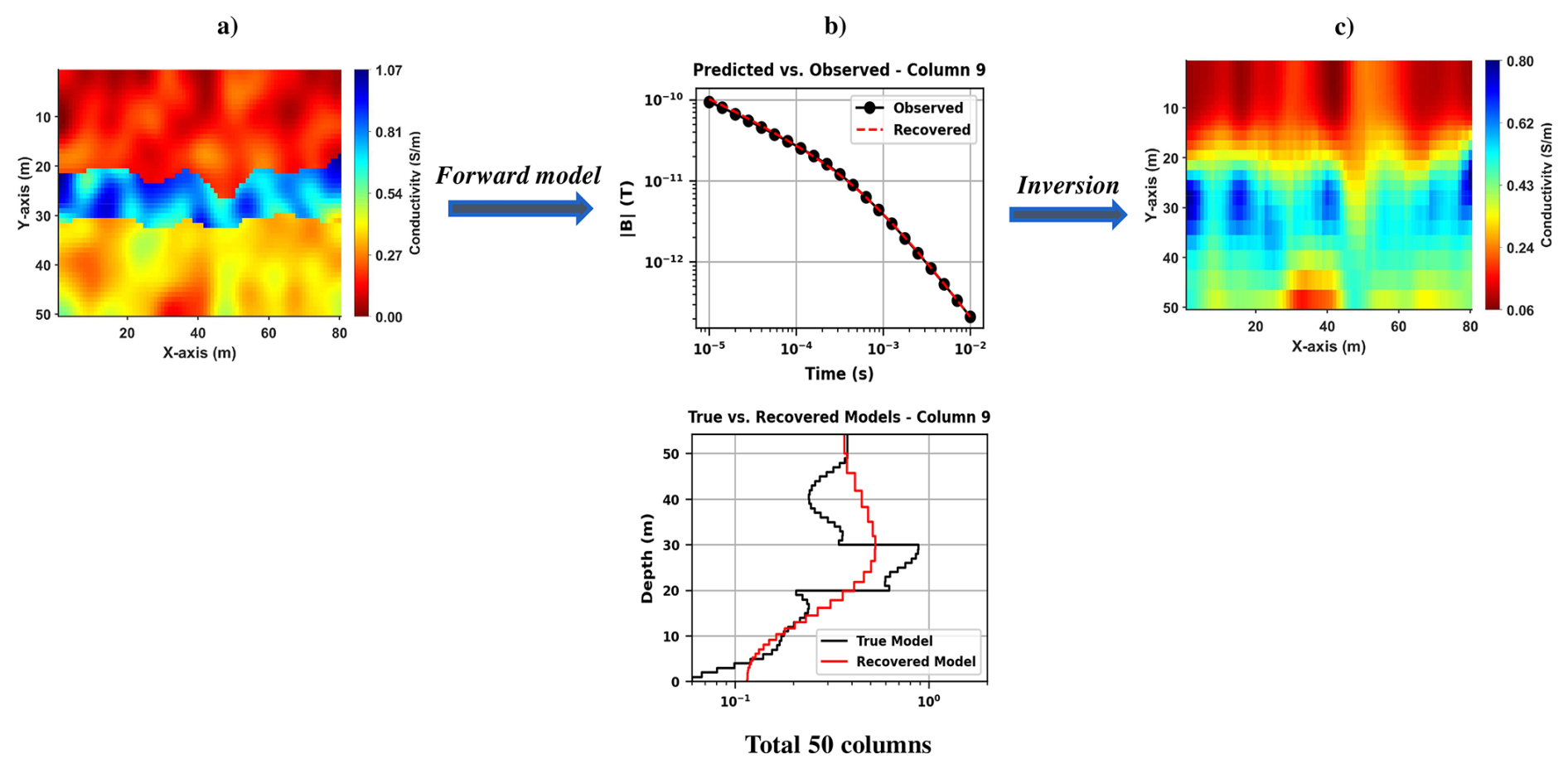
Figure 4 (a) True synthetic conductivity model constructed over 50 vertical soundings (columns) using random Gaussian distribution. (b) Both observed and recovered TEM responses for example of Column 9, and comparison between the true and inverted conductivity profiles (bottom). (c) Final stitched 2D conductivity section obtained by combining 1D inversion results for all columns.

3.1.3 Four simulation Scenarios

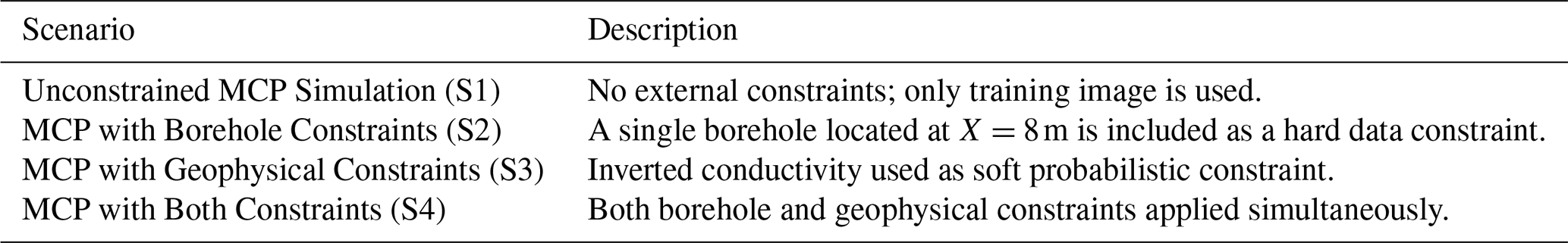
To evaluate the influence of different conditioning data types on the MCP framework, we designed four simulation scenarios whether or not incorporate borehole data and geophysical constraints in varying combinations (Table 2), which isolates the respective and combined impacts of boreholes and inverted geophysical data on lithological prediction.

Table 2 Simulation scenarios evaluated in the synthetic case.

For each scenario, 100 realizations were generated to assess the variability and consistency of the predicted lithological structures.

3.1.4 Synthetic Results

To evaluate how different constraints affect simulation results, we focus on the probability of predicting lithology category 2 across all realizations. In the synthetic case, no post-processing step is applied. Layer 2 was selected because it represents the central unit in this model, offering an indirect view on overlying and underlying layers. The results of the four scenarios are summarized in Fig. 5, which shows three realizations from each scenario, along with the probability distribution of lithology 2 based on 100 simulations.

In the first scenario at Table 2, no conditioning data were applied and the simulations were entirely driven by the spatial patterns from the training image. This led to considerable variability between realizations and a poor representation of the true model. Adding a single borehole in the second scenario significantly improved the simulation near the borehole. The model showed higher certainty in the vicinity of the hard data, and the predicted lithologies more closely matched the true values at those points. However, further away from the borehole, uncertainty remained high. The third scenario, which only introduced geophysical constraints, resulted in better large-scale continuity of the lithological units. Since the inverted resistivity model provides spatially distributed information, the simulation was able to capture broader geological trends, even though some details between the second and third layer remained somewhat uncertain, which reflects the loss of resolution with depth for TEM data. In the final scenario, where both borehole and geophysical constraints were used, the simulation achieved the best overall performance. The combination of point-based hard data and spatially distributed soft information led to more accurate and geologically consistent results. The realizations were more stable across the entire domain, and the predicted lithological patterns closely followed the structure of the synthetic true model.

In conclusion, the synthetic results from Fig. 5 demonstrate the complementary roles of hard and soft conditioning data. Borehole constraints effectively suppress simulation artifacts and enforce stratigraphic consistency, whereas geophysical constraints improve structural resolution, particularly in the delineation of transitional layers such as layer 2. However, when applied in isolation, soft constraints may lead to overconfident yet geologically implausible realizations. This emphasizes the need to integrate both data types within the MCP framework to achieve simulations that are both structurally accurate and geologically realistic. Moreover, although MCP has the property of enforcing hydrostratigraphical ordering, the incorporation of soft constraints from geophysical data may still result in local violations of this ordering. Therefore, in the following real-field application, a post-processing step, as described in Sect. 2.3, is necessary to ensure geological plausibility.

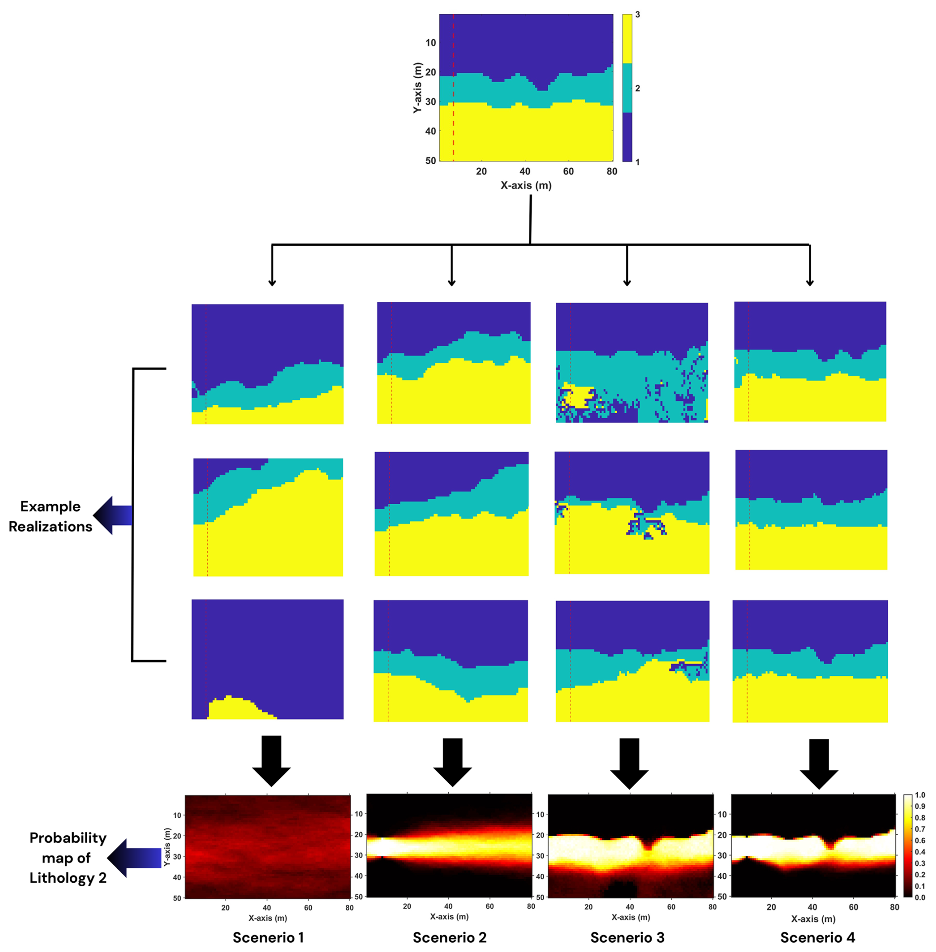
Figure 5 Example realizations (top three rows) and probability distribution of lithology 2 (bottom row) based on 100 simulations under four constraint scenarios (no post-process step for synthetic case).

3.1.5 Sensitivity analysis of the geophysical constraint

As demonstrated in the previous results, realizations generated using the MCP framework alone strictly adhere to geological ordering constraints. However, in regions lacking hard conditioning data, the simulations tend to revert to more uniform or overly smoothed patterns. In contrast, realizations influenced solely by geophysically derived conditional probabilities exhibit greater local variability but often lack spatial coherence. To explore this trade-off, a sensitivity analysis for the parameter τ (which governs the relative influence of geophysical data in Eq. (5) was conducted.

Introducing the Jaccard similarity index, J(S,R), which quantifies the overlap between the true model dataset S and a single realization R:

$$\begin{array}{}\text{(11)}& J(S,R)={\displaystyle \frac{|S\cap R|}{|S\cup R|}}.\end{array}$$

Based on this definition, the corresponding Jaccard dissimilarity is defined as:

$$\begin{array}{}\text{(12)}& U(S,R)=\mathrm{1}-J(S,R),\end{array}$$

which reflects the degree of mismatch between two categorical maps. To assess the overall variability across multiple realizations, the averaged Jaccard dissimilarity is computed as:

$$\begin{array}{}\text{(13)}& \stackrel{\mathrm{‾}}{U(S,R)}={\displaystyle \frac{\mathrm{1}}{n}}\sum _{i=\mathrm{1}}^{n}U(S,R_i).\end{array}$$

Figure 6 presents the Jaccard dissimilarity for the different importance of geophysical data introduced, reinforcing the effectiveness of moderate geophysical weighting. As shown in Fig. 6, the averaged Jaccard dissimilarity decreases as τ increases to a certain point, indicating an improved agreement between the simulations and the true model. The minimum dissimilarity is achieved at τ≈3, beyond which further increases in τ do not significantly improve model accuracy and may even lead to a little bit over-reliance on potentially noisy geophysical data. However, once τ becomes sufficiently large, the influence of varying τ values on the simulation results stabilizes. These results indicate that assigning a relatively high geophysical weighting τ within the MCP framework can lead to improved agreement with the true lithological model. Although excessive weighting may introduce minor inconsistencies, the overall performance remains good. This finding provides the guidance for the following real-field applications in areas with sparse borehole data, where assigning a relatively higher geophysical weight may effectively enhance model performance.

Figure 6 Sensitivity of weight of geophysical constraint in MCP via averaged Jaccard dissimilarity.

3.2 Real-case application

3.2.1 Study area

The study area is located near Egebjerg in Jylland, Denmark, and covers approximately 150 km² (Fig. 7). It is situated in a glacially influenced landscape characterized by a complex subsurface geological setting, where buried valleys, discontinuous aquitards, and interbedded sand and clay units contribute to significant spatial heterogeneity. The surface geology is primarily composed of clayey tills, with terrain elevations reaching over 160 m above sea level (Madsen et al., 2022). The study area has been interpreted using a stratigraphic model comprising 14 hydrostratigraphic units, ranging from Quaternary sediments to Danian limestone (Table 3). This parameterization follows the standard stratigraphic framework adopted in the national Danish hydrostratigraphic model (Jørgensen et al., 2010a). In particular, Layers $\mathrm{5},\mathrm{6},\mathrm{7},\mathrm{8}$ and 9 in Table 3, which consist of Quaternary sand and clay deposits, are commonly found within buried valley structures and are known to exhibit irregular thicknesses and discontinuities (Jørgensen et al., 2010b; Sandersen and Jørgensen, 2017). These features present challenges for the subsurface modeling due to their highly variable nature and the limited availability of deep conditioning data.

Borehole lithological information was obtained from the Danish national borehole database, Jupiter, which includes 794 boreholes within the study area (Hansen and Pjetursson, 2011). However, approximately 78 % of these boreholes are shallower than 50 m (Ter-Borch, 1991). To complement the limited borehole coverage, airborne transient electromagnetic (TEM) data from the SkyTEM system were utilized. These data were acquired along flight lines spaced 150 to 250 m apart, providing dense spatial coverage across much of the area (Madsen et al., 2022; Sørensen and Auken, 2004).

Table 3 Lithological layers in the catchment with descriptions (adapted from Madsen et al., 2022).

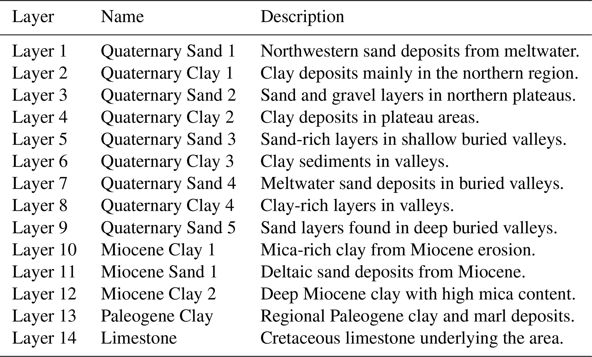
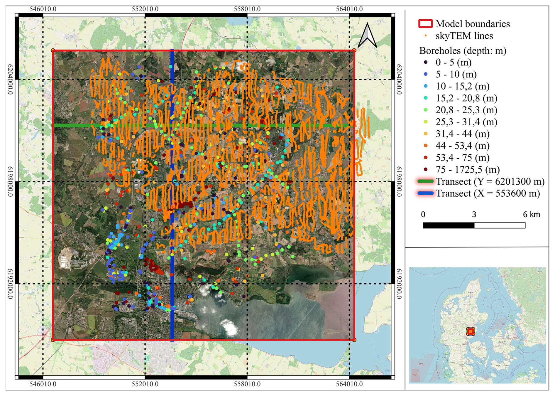
Figure 7 Distribution of boreholes and SkyTEM flight lines in the study area near Egebjerg, Denmark. The airborne electromagnetic data provide dense spatial coverage across the region in the central and northeastern parts. The red frame outlines the boundary of the previously established 3D model, which is used as a reference model for training image extraction. Borehole data are mostly shallow, with the majority of boreholes reaching depths of less than 50 m. Two highlighted transects X=553 600 UTM and Y=6 201 300 UTM were selected for detailed analysis. Both transects include segments with limited borehole data coverage. (Base map © OpenStreetMap contributors 2026, distributed under Open Database License (ODbL) license).

3.2.2 Interpreted model and selection of TIs

The 3D geological model of the study area was established by a cognitive hydrostratigraphic model, which integrates borehole data, geophysical surveys and geological interpretations (Enemark et al., 2022; Madsen et al., 2022). This model serves as a reference for training image generation and uncertainty assessment. This 3D geological model as shown in Fig. 8 is originally a layer-based model without regular discretization in the vertical direction. In this study, we impose a uniform grid on the model domain, with horizontal extents from X=546 600 to 564 300 m and Y=6 188 700 to 6 205 700 m in 100 m intervals, and vertical discretization from elevation Z=80 to −100 m in 5 m intervals. Structurally, the hydrostratigraphic model consists of 13 geological boundaries that separate six aquifers (primarily Quaternary and Miocene sands) from seven aquitards (composed mainly of clays and marls). These layers presented at Table 3 extend from the top-limestone surface, which ranges from −120 m elevation in the north, to −550 m in the south, to the terrain surface (Jørgensen et al., 2010b; Ter-Borch, 1991). Figure 8 shows the 3D interpreted model along with representative 2D transects. This model is used as the basis for extracting training images, which are then used to constrain the MCP simulations and guide the generation of realistic geological realizations.

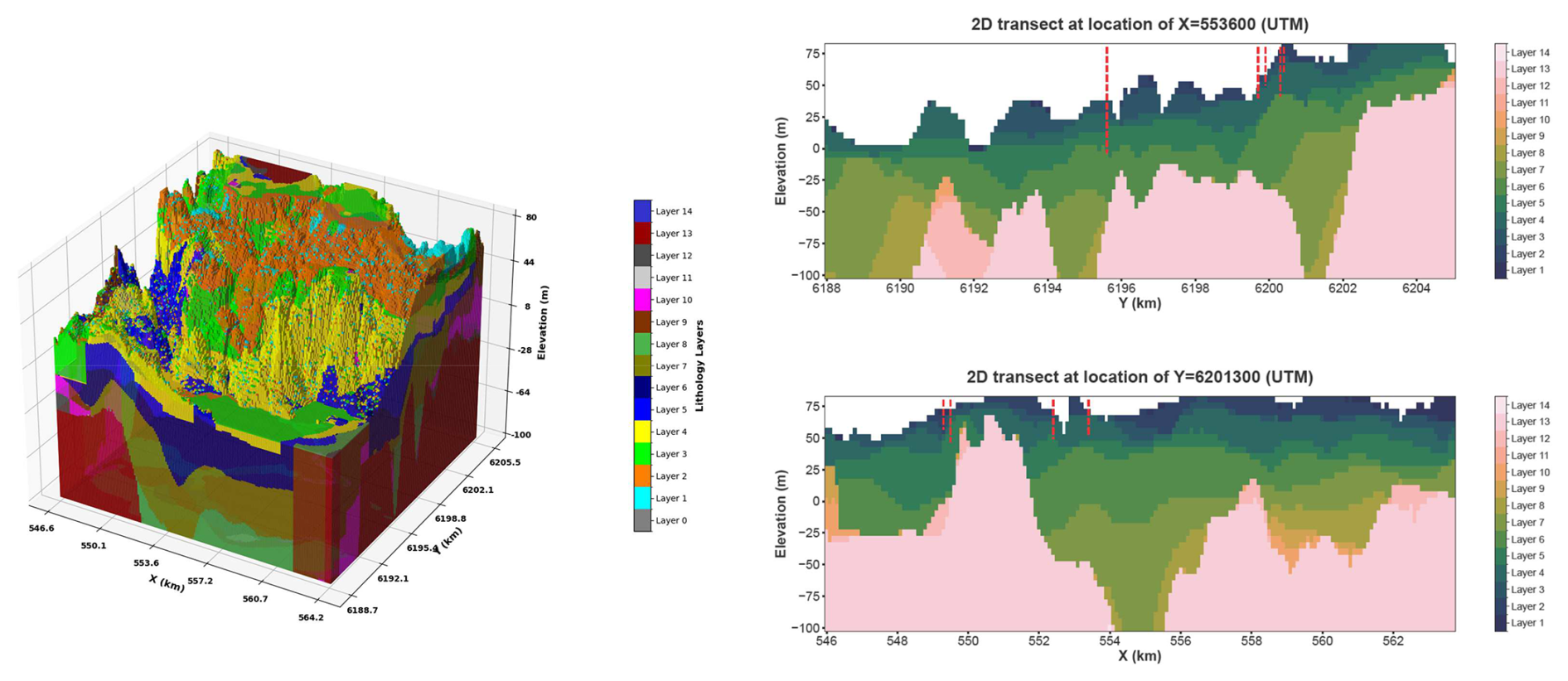
Figure 8 Interpreted 3D geological model used as prior information for training image extraction (left), selected 2D transect at X=553 600 m (right top), and selected 2D transect at Y=6 201 300 m (right bottom) used for detailed MCP simulation analysis. Red dashed lines indicate borehole locations and their depth extent.

The TI plays a central role in the MCP framework, as it is used to derive the bivariate transition probabilities $p_{i_k,i_{\mathrm{0}}}$, which describe the spatial relationships between lithological categories. Since a complete 3D TI is often unavailable in practice, we instead extract 2D transects from the interpreted 3D model. The transects are extracted every 400 m along both the x and y directions, resulting in 45 slices in the x direction and 43 in the y direction. This uniform sampling provides homogeneous coverage of the entire study area, ensuring that the main spatial variability and layering patterns present in the prior geological model are adequately represented. These 88 transects are then used to derive the bivariate transition probabilities required by the MCP algorithm.

To integrate the spatial information from the different individual transects into a single representative set of bivariate probabilities, we apply the Extended Logistic Opinion Pool (ELOP) method (Satopää et al., 2014). ELOP combines multiple probability estimates in a statistically consistent way, enabling the aggregation of directional spatial patterns while preserving variability.

$$\begin{array}{}\text{(14)}& \widehat{p}={\displaystyle \frac{{\prod }_{i=\mathrm{1}}^N{p}_i^{w_i}}{{\prod }_{i=\mathrm{1}}^N{p}_i^{w_i}+{\prod }_{i=\mathrm{1}}^N(\mathrm{1}-p_i{)}^{w_i}}},\end{array}$$

where p_i represents the bivariate probability derived from each individual 2D transect, and w_i is the corresponding weight assigned to each bivariate probability, here equal weights are assigned to all transects.

The resulting unified 2D probability dataset is then used as input for MCP simulations across the entire model domain. Figure 9 shows an example of the integrated bivariate probability distribution P(i,j) at different locations, where both i and j correspond to lithology 12, constructed from all 88 extracted transects using the ELOP function. Hence, the integrated bivariate probability serves as prior spatial information for all transects of the 3D model and enables the construction of a full 3D lithological simulation by applying the MCP framework across each transect sequentially.

Two 2D transects are extracted from the interpreted 3D geological model: one aligned along X=553 600 m and the other along Y=6 201 300 m. These transects are selected in zones characterized by limited borehole coverage and variable SkyTEM data availability, which are typical of areas where conventional modeling approaches often struggle to represent complex geological features. The spatial variability along these transects, especially the presence of buried valleys and heterogeneous stratigraphic transitions, provides a interesting test case for the MCP framework. While MCP has demonstrated robust performance in synthetic cases with relatively uniform stratigraphy (Benoit et al., 2018), its effectiveness in capturing highly variable geological features in real-world applications depends heavily on the quality and density of available constraints.

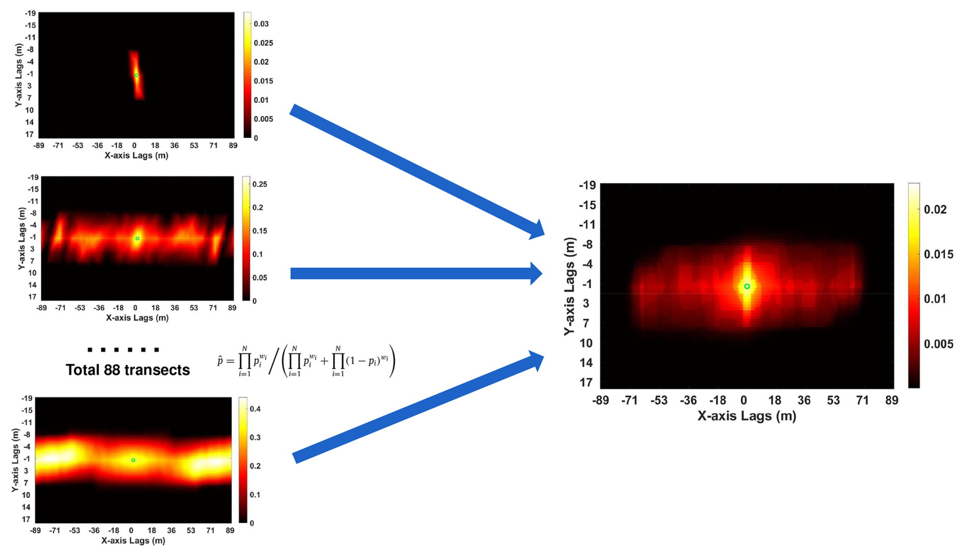
Figure 9 Bivariate transition probabilities P(i,j), where i and j represent the 14 lithological layers, were derived from 88 transects extracted from the 3D interpreted model. These were then merged into a single generalized 2D bivariate probability distribution using the Extended Logistic Opinion Pool (ELOP) method. This unified distribution can be applied across all 2D transects. Shown here is an example for P(12,12) illustrating the spatial relationship aggregated from all 88 transects.

3.2.3 Geophysical data

For this case, we used the existing resistivity model obtained from the inversion of SkyTem data to characterize the subsurface structure. The TEM data were collected along flight lines spaced between 150 and 250 m, providing comprehensive spatial coverage. Data acquisition involved transmitting electromagnetic pulses into the ground, with the subsequent decay of induced currents measured to detect variations in electrical resistivity (Sørensen and Auken, 2004). Early-time decay measurements provided high-resolution information for shallow depths, while later-time measurements offered insights into deeper geological layers, enabling investigations down to depths exceeding 300 m. SkyTEM is particularly well-suited for this application due to its high spatial coverage, its sensitivity to both shallow and deep conductive structures, and its ability to detect subtle resistivity contrasts in layered sediments (Jørgensen et al., 2010b; Sandersen and Jørgensen, 2017).

Unlike the synthetic case, where a 1D inversion was used, the TEM data were inverted using the Laterally Constrained Inversion (LCI) method (Auken et al., 2005), which applies lateral constraints to ensure continuity between adjacent soundings, resulting in more geologically consistent resistivity profiles (Madsen et al., 2022). This is especially important in areas with only few available boreholes, as it reduces inversion artifacts and noise (Høyer et al., 2015; Jørgensen et al., 2015). Moreover, to honor the original field data, we have derived the statistical relation between lithology and resistivity ($\mathrm{\Omega }\mathrm{m}=\mathrm{1}/\left(\mathrm{S}{\mathrm{m}}^{-\mathrm{1}}\right)$), instead of conductivity as in Sect. 3.1.

To establish a statistical relationship between borehole information and the inverted resistivity model, resistivity values along each borehole depth profile are first estimated by applying linear interpolation using measurements from nearby SkyTEM flight lines (Fig. 10). As shown in Fig. 10c, the resistivity distributions associated with different lithological classes exhibit significant overlap. This makes it challenging to distinguish between lithologies based on resistivity alone. To improve it, depth is introduced as an additional conditioning dimension. To estimate conditional probabilities of lithology given resistivity, the interpolated resistivity values are statistically linked with lithological classifications and depth values from the boreholes. This is formulated as:

$$\begin{array}{}\text{(15)}& P(\text{lithology}\mathrm{|}\text{depth},\text{resistivity})={\displaystyle \frac{P(\text{lithology},\text{depth},\text{resistivity})}{P(\text{depth},\text{resistivity})}}\end{array}$$

However, since the study area contains only a few deep boreholes, direct sampling of conditional probabilities from sparse data can introduce considerable noise and lead to unstable estimates. To address this, and to ensure a more robust and continuous estimation of the borehole–resistivity relationship, Kernel Density Estimation (KDE) is employed instead of simple histogram based sampling (Manrique et al., 2024). By modeling the joint probability distribution in a continuous probabilistic framework, KDE helps smooth out local variability, thereby yielding more reliable conditional probabilities in data-sparse zones. The KDE bandwidth is determined using the normal reference rule, a standard data adaptive bandwidth selection method that computes the bandwidth from the sample covariance and the number of data points in each lithology class (Hall et al., 1991). The resulting conditional probability distributions for each lithological unit are shown in Fig. 11.

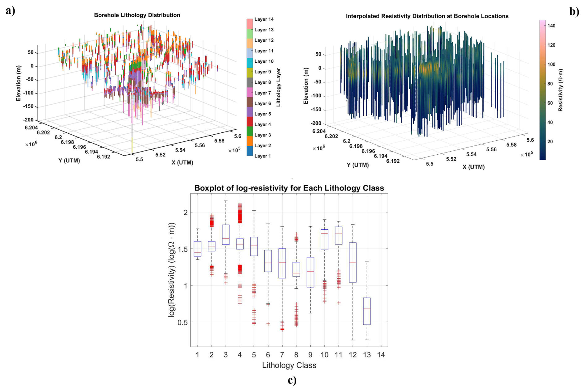
Figure 10 (a) Lithological information of each borehole. (b) Inverted resistivity values are interpolated along the borehole locations. (c) Inverted resistivity distribution with each lithology type based on interpolated resistivity values.

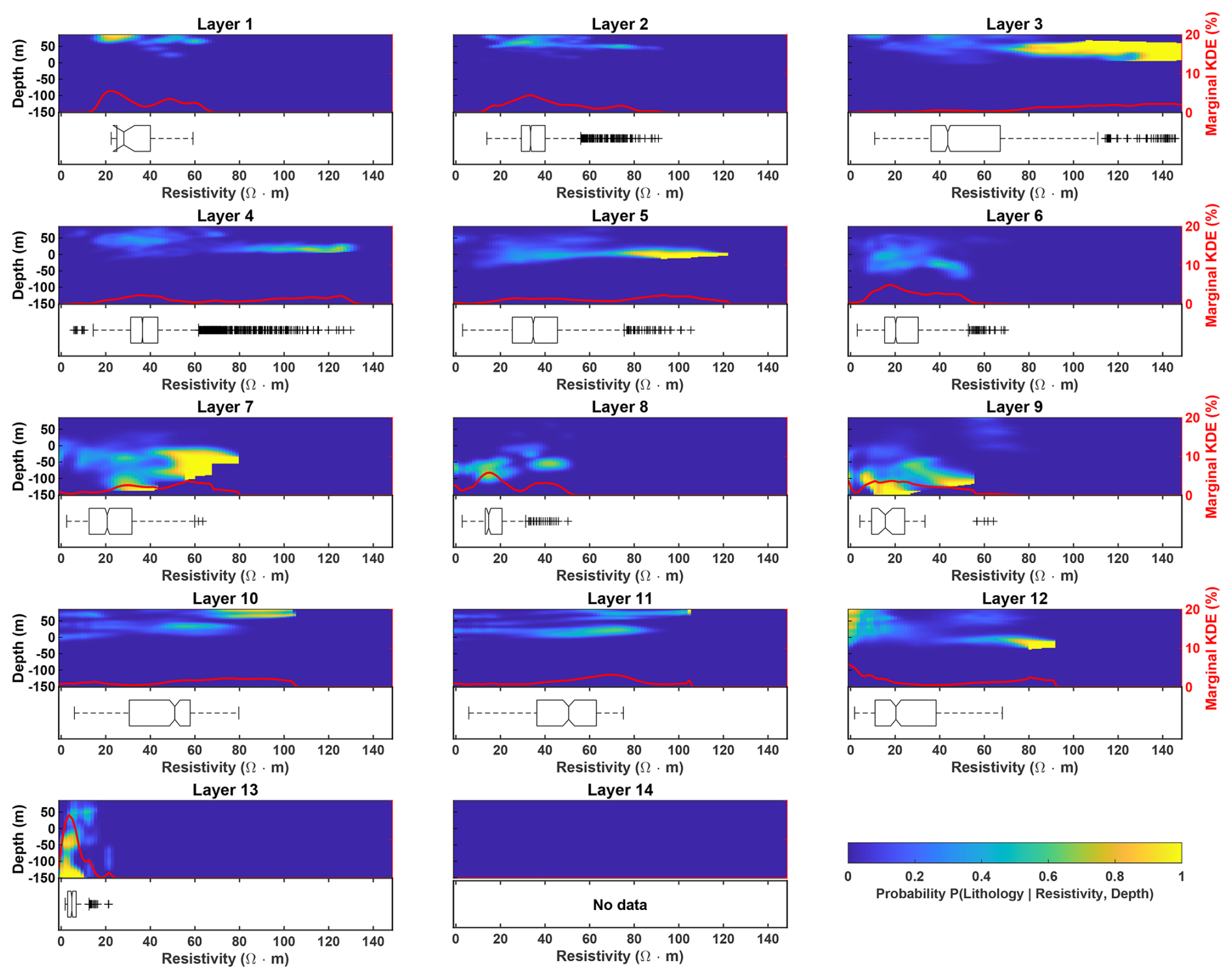
Figure 11 The heatmaps present the smoothed probabilistic distributions of each lithological layer estimated via KDE, conditioned on resistivity and depth. The red lineplot in each subplot represents the global normalized marginal probability of lithology conditioned solely on resistivity, derived from the KDE results. The boxplots below each heatmap display the distribution of resistivity values at each layer based on inverted geophysical data at borehole locations.

3.2.4 Workflow for the field case

The modeling workflow for the real-case application is summarized and illustrated in Fig. 12. The first step is to extract prior geological information from different transects of a 3D interpreted model, which are used to derive bivariate transition probabilities that represent spatial relationships between lithological units. The second step involves deriving a stochastic relationship that links borehole lithologies and their depths with resistivity values interpolated from the inverted model at borehole positions, using the neighboring TEM soundings. The final step is to integrate both geological expert knowledge represented by the TI and geophysical information using the permanence-of-ratios principle (Eq. 5) within the MCP framework. In this specific application, a weighting factor of τ=0.11 is assigned to the MCP prior term (b). This fixed value was chosen to balance the contribution of the prior knowledge, acknowledging that the reliability of MCP-derived probabilities is spatially constrained due to the relatively shallow borehole coverage (<50 m). This adjustment is determined through an iterative trial-and-error process and enables the generation of geologically realistic lithological realizations constrained by both borehole and geophysical data.

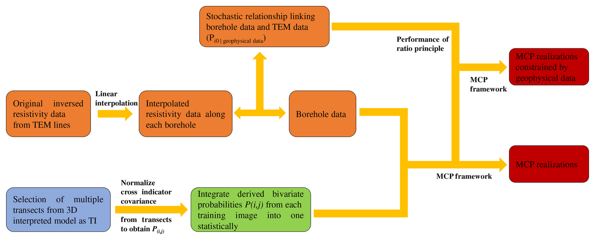
Figure 12 Workflow for the real-world field application in Egebjerg, Denmark. The orange boxes represent the processing of geophysical data and the derivation of stochastic relationships between lithology and resistivity at borehole locations. The purple and green boxes denote the selection of multiple 2D transects from the 3D interpreted model to statistically integrate bivariate transition probabilities. The red boxes indicate the final simulation outcomes, enabling a direct comparison between baseline MCP realizations and posterior realizations generated from the extended MCP framework with integrated geophysical constraints.

3.2.5 Simulation results of real-case study

The simulation results for the selecting transects are presented for two scenarios: (i) using only the training image and borehole data, and (ii) incorporating additional geophysical constraints derived from interpolated resistivity profiles.

Figures 13 and 14 present two example realizations for each scenario at both two transects, more realizations can be seen in Appendix A. As shown in Figs. 13a–b and 14a–b, in the absence of geophysical constraints and with limited hard data (borehole) support, the MCP simulations tend to produce more simplified and uniform stratigraphic configurations. This tendency is particularly evident in the limited presence of buried valley features, typically associated with Layers 5 to 9. These valley layers are poorly delineated, with simulated transitions between lithologies appearing diffuse and inconsistent with the expected buried valley morphology. The associated entropy maps (Fig. 15) for two transects indicate the tendency of all simulations to produce overly uniform or vertically stacked layers in regions lacking hard conditioning data. Nevertheless, the MCP framework still effectively maintains the stratigraphic ordering of lithological units, ensuring that the simulated realizations respect the geological age relationships encoded in the training image and conditioning data.

By contrast, when geophysical constraints are introduced (c–d of Figs. 13 and 14), the simulations demonstrate markedly improved spatial variation and yield realizations that are more geologically consistent and closely match the existing reference model (right of Fig. 8). Buried valleys, in particular, are more clearly defined, and the geometries of Layers 5–9 show better agreement with the interpreted stratigraphy. In particular, based on the probability maps of each layer obtained from 100 simulations at Figs. 16 and 17, Layer 7 are more spatially continuous and correspond well with high-resistivity zones from the inverted AEM data. The probability distributions also reflect this improvement, with values often exceeding 0.8 in areas where a specific layer is expected to occur, indicating higher model confidence. The entropy maps (Fig. 15) further confirm that the inclusion of AEM resistivity data enables sharper delineation of complex subsurface features and significantly improves lateral continuity across stratigraphic boundaries.

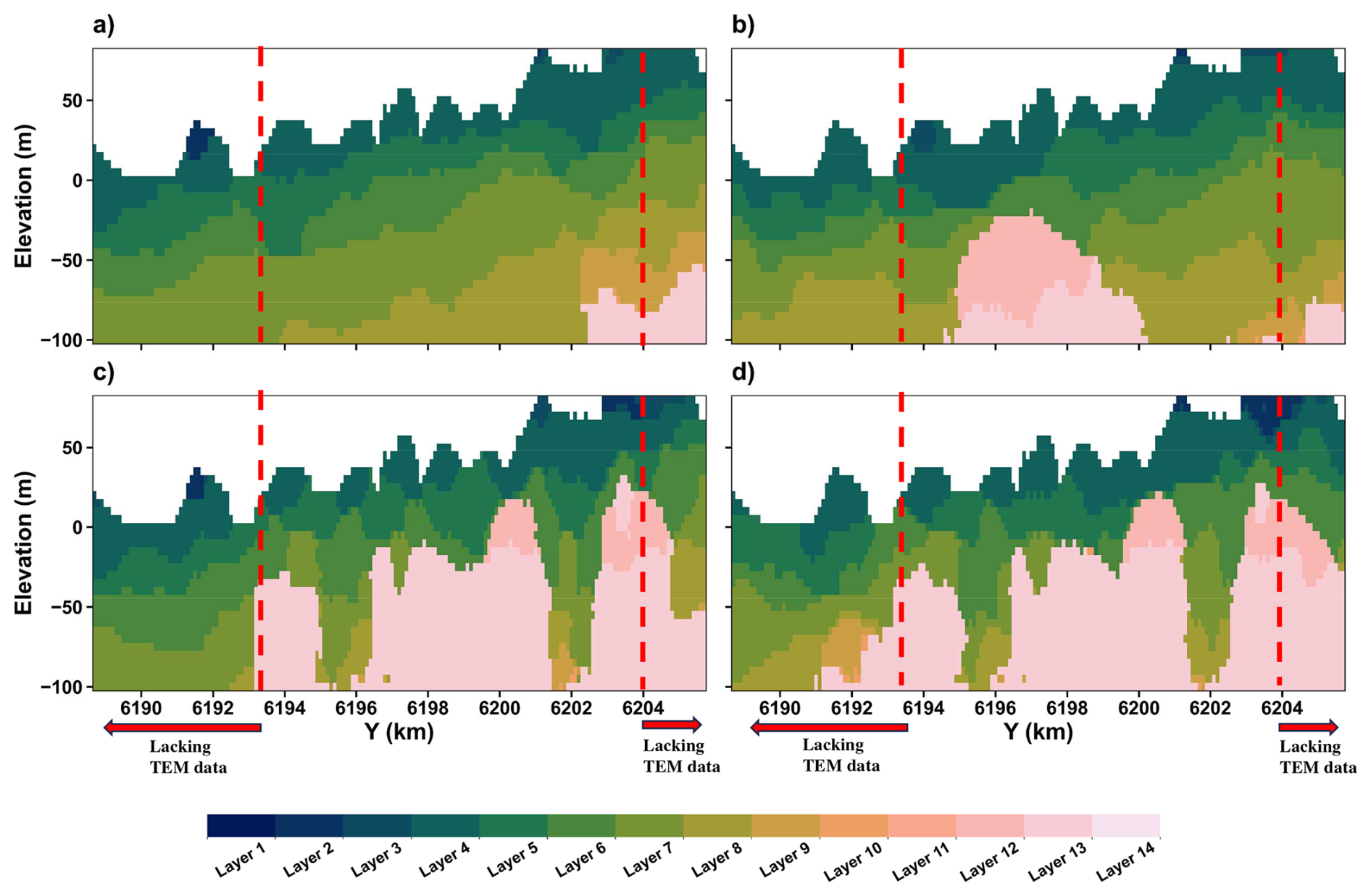
Figure 13 Modeling performance at transect of X=553 600 (UTM), red dash lines represents the boundary of existence of TEM data: (a, b) wo example realizations from MCP simulation without geophysical constraint. (c, d) Two example realizations from MCP simulation adding geophysical constraint.

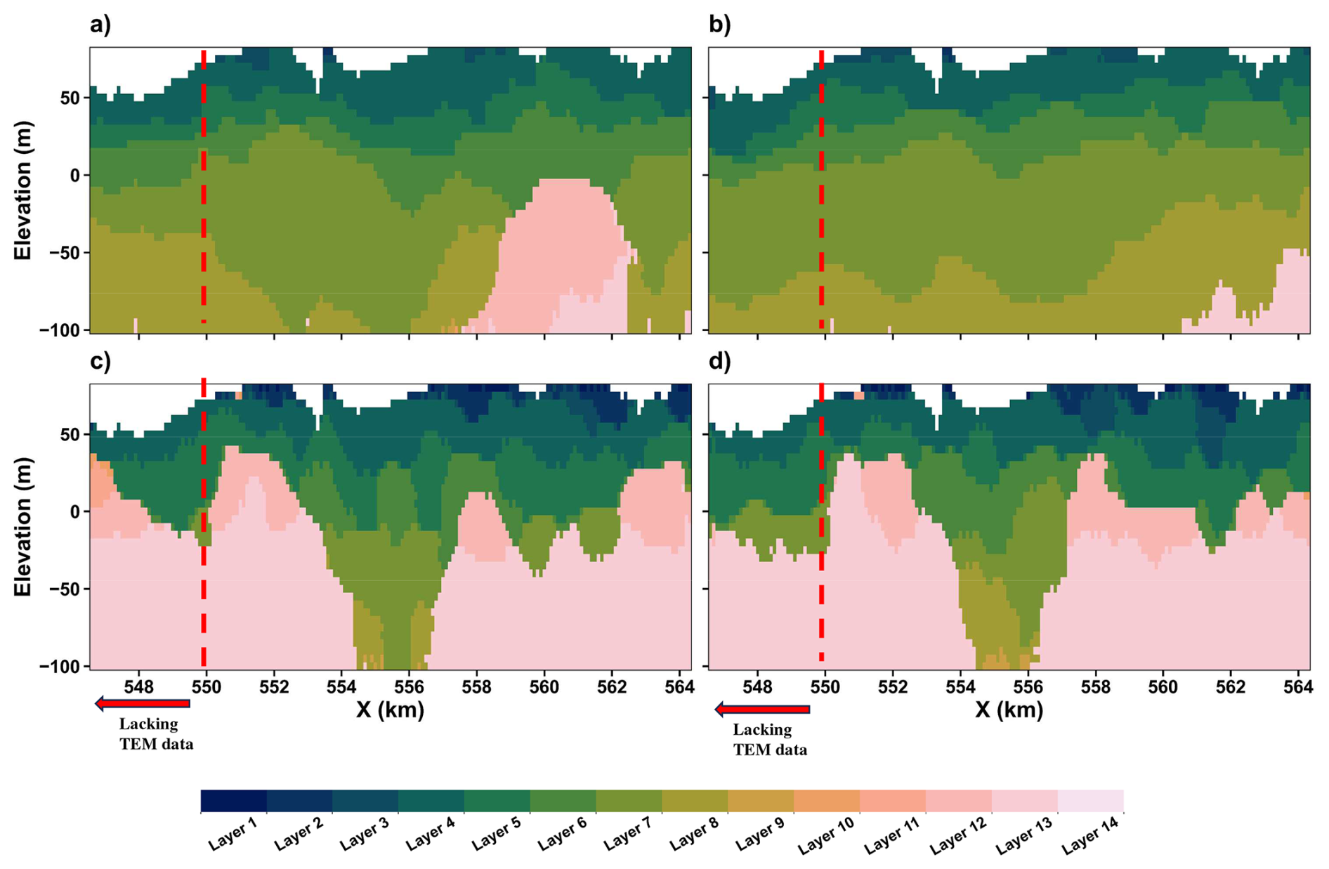
Figure 14 Modeling performance at transect of Y=6 201 300 (UTM), red dash lines represents the boundary of existence of TEM data: (a, b) Two example realizations from MCP simulation without geophysical constraint. (c, d) Two example realizations from MCP simulation adding geophysical constraint.

The entropy maps (Fig. 15) provide insight into the spatial distribution of predictive uncertainty across the model domain. In areas where lithological predictions are consistent across realizations, entropy values are low, whereas higher entropy reflects increased variability between simulated outcomes. As expected, laterally continuous units, such as the deeper clay layers, are generally associated with low entropy, indicating that these structures are well constrained by the available data. In contrast, higher entropy is mainly observed along the boundaries of buried valleys. These zones correspond to abrupt lithological transitions and complex erosional geometries that are difficult to resolve precisely, particularly in the absence of deep borehole information. Importantly, the concentration of higher entropy along valley boundaries suggests that the buried valley geometry is being identified, while uncertainty remains confined to geologically plausible transition zones rather than being distributed randomly across the model. When geophysical constraints are incorporated, the entropy patterns become more spatially structured, with low entropy dominating the continuous clay units and higher values restricted to valley boundaries. Without geophysical constraints, entropy remains high over much larger portions of the domain, and the buried valley structure is poorly expressed. Thus, the entropy maps complement the lithology realizations by demonstrating that the soft constraints help recover the buried valley feature, while also revealing how uncertainty is distributed consistent with expectations based on the geological information.

It is important to note that the impact of geophysical constraints is not uniform across the transects as can be seen in the spatial distribution of boreholes and SkyTEM flight lines in the study area (Fig. 7). In areas where resistivity data coverage is dense, the MCP realizations show significant reductions in uncertainty and more geologically plausible transitions. However, in peripheral regions or at the edges of the model domain where resistivity coverage is sparse or absent (see indicated areas on Fig. 15, uncertainty remains high, and the model reverts to patterns driven primarily by the TI. What distinguishes the MCP framework, however, is its ability to transition smoothly between data-constrained zones and prior-based inference through its probabilistic treatment. This is made possible by its sequential simulation process, where simulated values in well-constrained areas are progressively used as new conditional data for simulating the remaining parts of the model. This mechanism allows local observations to gradually influence larger domains, providing a probabilistically coherent integration of observed data and prior geological structure.

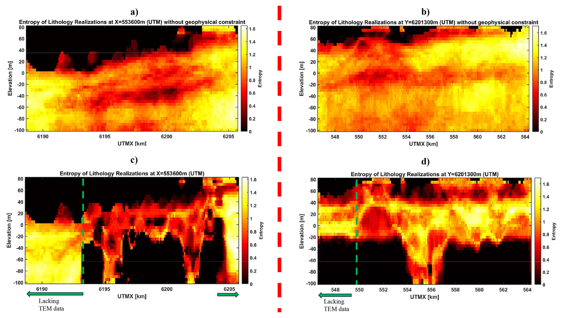
Figure 15 Uncertainty analysis based on entropy values, green dashed lines represent the boundary of existence of TEM data: (a, c) Entropy maps based on MCP realizations along the transect at X=553 600 (UTM). (a) shows the case without geophysical constraints, while (c) shows the case with geophysical constraints. (b, d) Entropy maps based on MCP realizations along the transect at Y=6 201 300 (UTM). (b) shows the case without geophysical constraints, while (d) shows the case with geophysical constraints.

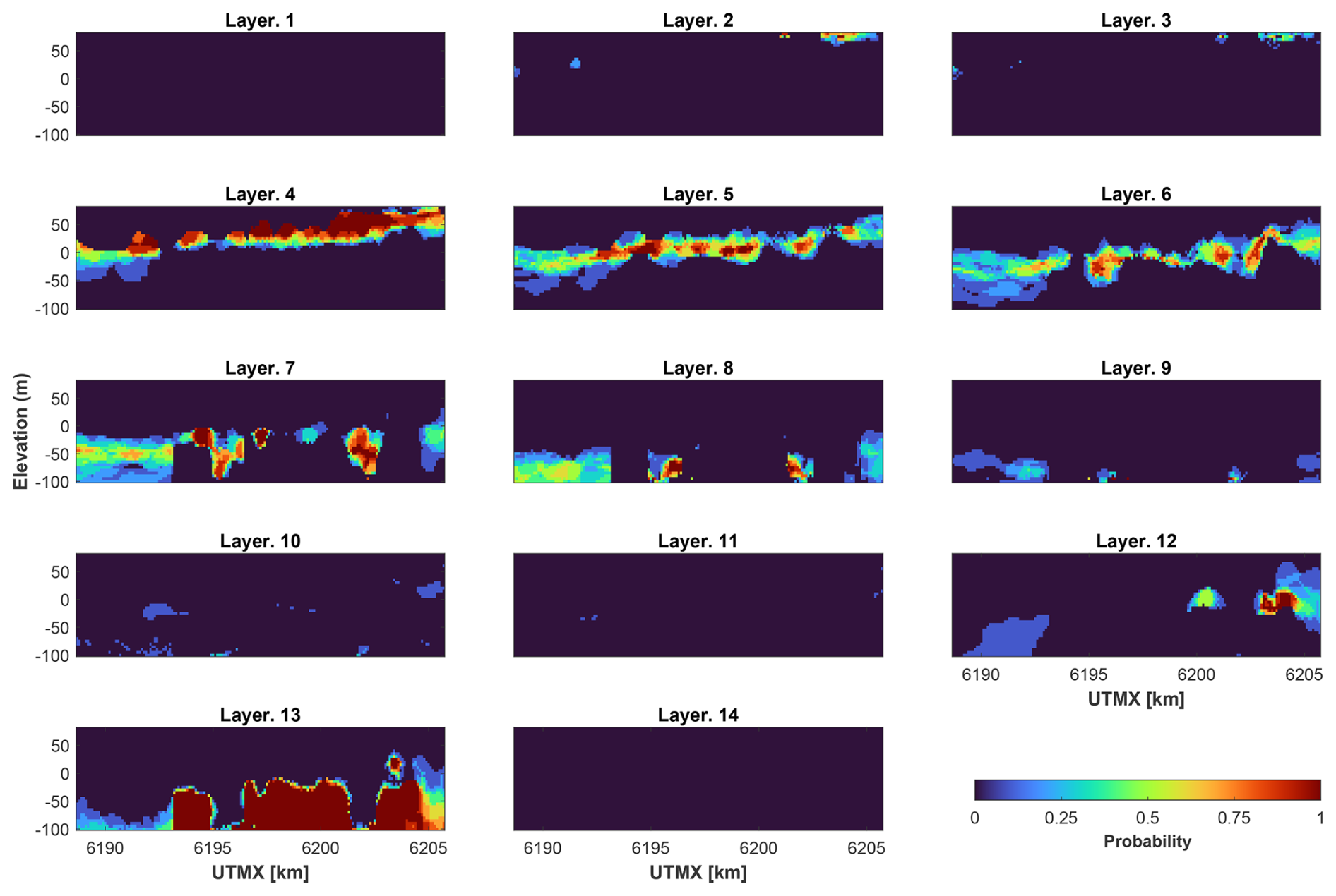
Figure 16 Probability distribution of each lithological layer in each pixel from 100 MCP simulations with geophysical constraints for transect of X=553 600 (UTM).

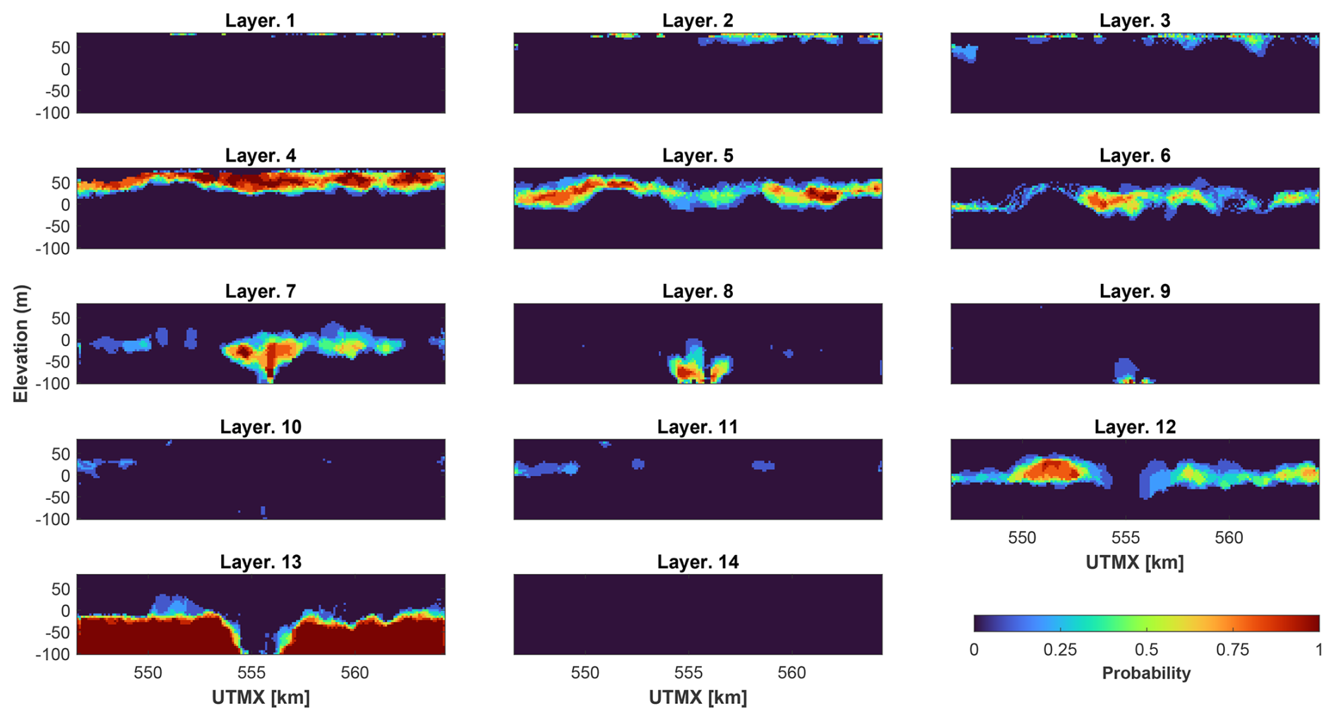
Figure 17 Probability distribution of each lithological layer in each pixel from 100 MCP simulations with geophysical constraints for transect of Y=6 201 300 (UTM).

4 Discussion

To better understand how our novel MCP framework with geophysical constraints better captures lithological proportions, a comparison plot was produced using the transect at Y=6 201 300 m as an example (Fig. 18). It evaluates the consistency and variability in the simulated lithology proportions across multiple realizations, and how these compare with the TIS and the lithological composition of the target transect. The overall facies proportions derived from the TIs are generally comparable to those realizations obtained with geophysical constraints, suggesting broad consistency in global distributions. However, several lithological units show noticeable inconsistencies between the simulated proportions and those derived from the TIs. For example, Layer 4 and Layer 12 are clearly overrepresented in the MCP realizations compared to their occurrence in the TIs. This overestimation is likely influenced by a few deep boreholes in the transect area, causing a strong local constraint during simulation. In contrast, Layers 6, 7 and 8 appear to be underrepresented in the simulations. These lithologies are associated with deep valley structures in the geological model. However, due to the limited number of deep boreholes in these areas, the available hard conditioning data are sparse or entirely absent. In the absence of geophysical data, the probability values derived from the framework are insufficient to capture and preserve the complex geometry of these buried valleys. The framework tends to favor a more uniform stratification, leading to a reduced occurrence of these deeper facies in the realizations (Benoit et al., 2018). Nevertheless, the integration of geophysical constraints helps to simulate these structures. While it does not significantly alter the proportions, it successfully limits unrealistic deviations and maintains reasonable spatial consistency in the valley zones.

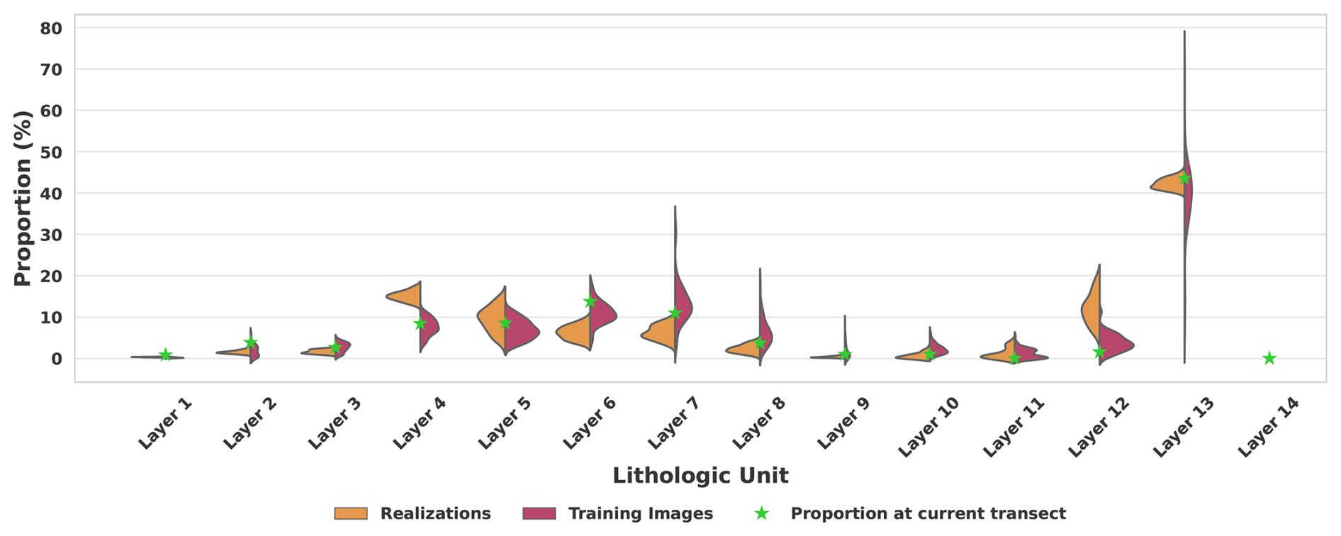
Figure 18 The orange bars on the left side show the distribution of proportions across multiple MCP simulation realizations with constraint from geophysical data, the red bars on the right side represent the distribution derived from the 88 different training images, and the star markers indicate the mean proportion of each lithology observed in the current target transect from interpreted model.

It is essential to examine closer the role of the choice of TI and how it influences the outcomes. A sensitivity analysis aims to evaluate the robustness of the MCP framework with respect to different TI selections and to determine the extent to which lithological predictions depend on the chosen TI.

To perform such analysis, 11 transects were randomly selected from the 88 available transects to serve as individual training images. For each selected TI, 100 realizations of the lithological model were generated using the MCP framework with geophysical constraints. The Jaccard dissimilarity index (Eq. 13) was calculated for each realization with respect to the interpreted geological model, providing a quantitative measure of dissimilarity between the predicted and reference models. In addition to these random selections, an integrated TI, constructed by combining information from all 88 transects, was used to produce another set of 100 realizations. Furthermore, a separate scenario was tested in which the target transect itself (Y=6 201 300 UTM) from the interpreted model was used as the TI. This setting, referred to as the “Best TI” in the results, uses as an idealized case where the training data perfectly reflect the spatial patterns of the target.

The results of this sensitivity analysis are presented in the Fig. 19, which displays the average Jaccard dissimilarity index for all 13 TI scenarios (11 random TIs, 1 integrated TI and one the target transect itself). Across all scenarios, the average dissimilarity values are remarkably similar, with minimal variation observed. This indicates that the lithological predictions remain consistent regardless of the TI selection. This observation is consistent with findings by Barfod et al. (2018), who used multiple-point statistics in combination with SkyTEM data and noted that the influence of the training image was significantly reduced when strong geophysical constraints were applied. In contrast, under the low geophysical constraint scenario, the influence of TI selection becomes larger. However, the overall variation in results remains small. This is primarily because the boreholes in the study area are shallow and provide minimal hard conditioning data. Consequently, the simulations generated using only the MCP framework, without incorporating geophysical information, rely largely on bivariate transition probabilities. These probabilities inherently preserve the expected stratigraphic ordering (e.g., older layers occurring at greater depths), leading to realizations that exhibit relatively uniform layering and limited structural variability. Notably, similar results were obtained when using an integrated TI compared to using the target transect alone, indicating that the ELOP based integration strategy performs reliably within the MCP framework.

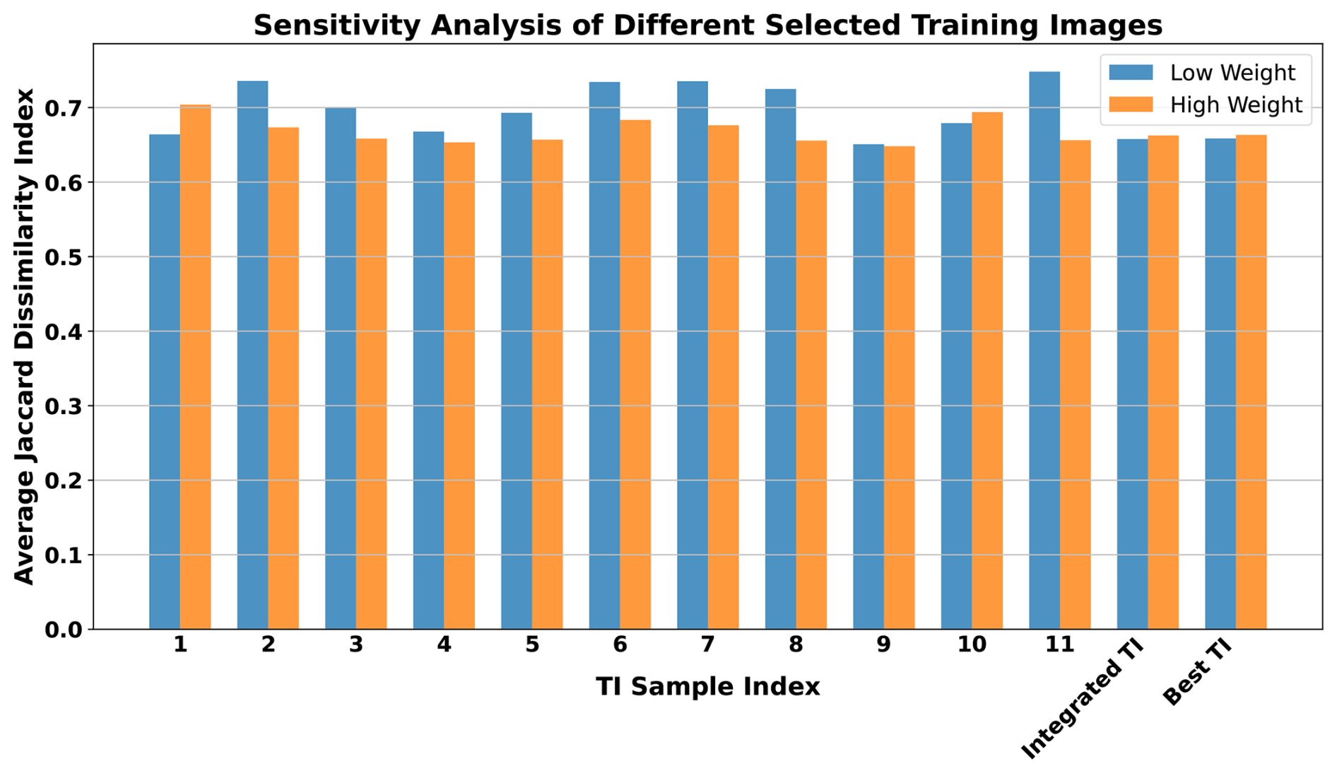
Figure 19 Sensitivity analysis of TI selection on lithological predictions using the MCP framework with geophysical constraints. The bar plot presents the average Jaccard dissimilarity index, computed over 100 realizations for each of the 13 TI scenarios, using the interpreted geological model shown in Fig. 7 as the reference model. These include 11 randomly selected TIs, one “Integrated TI” constructed from all 8 transects, and one “Best TI” using the current transect as the TI. Blue bars represent results under a low weight of geophysical constraint, while orange bars represent results under a high weight of geophysical constraint.

An important factor that influences the quality of lithology simulations is how geophysical resistivity data are acquired and processed (Rochlitz et al., 2023; Javed et al., 2019). In this study, the resistivity model was generated through the Laterally Constrained Inversion (LCI) method from airborne electromagnetic (EM) data and then interpolated along borehole paths to estimate continuous resistivity values with depth. Both steps introduce a degree of smoothing: the inversion averages resistivity over vertical windows, which tends to reduce sharp boundaries between lithological units, while interpolation smooths spatial variations further due to the distance between flight lines and boreholes. As a result, the resistivity values used to link with lithological categories do not fully capture the fine-scale variations of the true subsurface and may present a simplified or blurred version of reality. This smoothing directly affects the conditional probability distributions used in the MCP simulations. When resistivity contrasts between lithologies become less distinct, especially at depths where their values overlap, the probability curves become wider and their peaks less defined. This increases the uncertainty in lithology classification during simulation, particularly in zones where several units share similar resistivity ranges. More advanced inversion techniques (Deleersnyder et al., 2023) could potentially improve conditional probability from geophysical data as suggested in Hermans and Irving (2017).

In parts of the model where deep boreholes data are missing, the simulation process becomes more uncertain. Without hard information to constrain the deeper layers, MCP relies mainly on the training image and the overall proportion statistics, which may not reflect the specific conditions of the target area (Benoit et al., 2018). In this situation, the use of geophysical data becomes particularly helpful. Even though the resistivity model is smoothed due to inversion and interpolation, it still carries important signals about the general layering and structural trends at depth. By incorporating this resistivity information, the conditional probabilities in MCP are guided by more than just borehole data and facies proportions. This helps the simulation pick up on major features, such as buried valleys or sharp transitions that would likely be missed or misrepresented otherwise. As a result, geophysical constraints play a key role in maintaining geological plausibility in deeper zones where direct observations are lacking.

While no direct MPS simulations were performed in this study, a relevant comparison can be drawn from the work of Barfod et al. (2018), who applied MPS simulations for the same Egebjerg field site. In their approach, the inverted AEM data were transformed into categorical probability maps for a limited number of hydrostratigraphic units (three categories), which were then used as soft conditioning data in a direct sampling MPS framework. This allowed the geophysical constraints to influence the final model, but only indirectly, by treating the inverted resistivity as a secondary training image, rather than incorporating it through explicit probability distributions. By contrast, the MCP framework used in this study relies on statistically derived bivariate transition probabilities extracted from interpreted geological models. It also enables the combination of directional transition probabilities from multiple transects using the Extended Logistic Opinion Pool (ELOP) approach, allowing for a consistent probabilistic framework across directions. More importantly, MCP provides a transparent mechanism for integrating soft geophysical constraints via conditional probability functions, which capture the uncertainty, smoothing effects, and resolution loss associated with geophysical inversion. Unlike Direct Sampling MPS, which incorporates soft data through auxiliary images, the MCP framework treats soft constraints probabilistically and explicitly, making it particularly well suited for vertically ordered, non-stationary hydrostratigraphic settings. This flexibility in combining hard borehole data with soft geophysical information makes one of the key advantages of MCP in such contexts. For the Egebjerg field site, Madsen et al. (2022) also addressed uncertainty, but within the framework of a deterministic conceptual model primarily guided by expert interpretation and constrained geological assumptions. In contrast, the MCP based simulations presented in this study offers a probabilistic representation of uncertainty, grounded in data driven inference and stochastic modeling. Unlike sequential layer-based modeling which may require layer-by-layer corrections, MCP accounts for vertical dependencies through transition probabilities. This allows the model to naturally preserve expected stratigraphy during simulation, although at the cost of requiring post-processing after incorporating geophysical constraints, which slightly alters the posterior distribution. Nevertheless, the resulting realizations are more informative for probabilistic groundwater modeling.

In this study, depth is used as an additional conditioning variable in the estimation of lithology–resistivity conditional probabilities (Hermans and Irving, 2017). Although depth are relative to the surface elevation, it still represents a meaningful stratigraphic indicator in many sedimentary environments, where systematic vertical trends are commonly observed. When combined with geophysical properties such as resistivity, depth therefore provides an effective means of capturing first-order stratigraphic organization within the probabilistic framework. Depth, or elevation, is directly observed at all borehole locations and can be consistently integrated with AEM resistivity data over the entire study area. In principle, other physically meaningful variables, such as bulk density or porosity or other geophysical properties, could also be used to construct conditional probability relationships. However, they would only be relevant of they are broadly available at the field scale. Extending the framework to incorporate alternative conditioning variables remains a promising direction for future work when suitable datasets are available and can be readily accommodated by the permanence of ratios approach (e.g. Manrique et al., 2024).

The observed robustness to TI selection opens the possibility of using geological models, such as the interpreted 3D model of the Egebjerg catchment, as generalized training images for simulating similar geological settings in neighboring regions. This would allow for more efficient modeling efforts over a wider spatial scale without the need to generate customized training images for each new site. However, this generalization relies heavily on the availability of dense and high-quality geophysical data (e.g., SkyTEM). In addition, the post-processing corrections contribute to how informative the geophysical constraint becomes. These choices play a crucial role in enabling the geophysical data to compensate for potential mismatches between the TI and the target area.

5 Conclusion and Prospective

Hydrostratigraphic modelling is a complex task as it requires to interpret information from sparse boreholes, leading to large uncertainty. In this context, geophysical data brings spatially distributed but indirect information to help interpolating stratigraphic units across boreholes. In this study, we developed an enhanced Markov-type Categorical Prediction (MCP) framework that integrates airborne electromagnetic (AEM) geophysical data as soft probabilistic constraints to generate lithological realizations. Through both synthetic and real-world case studies, we demonstrated that the inclusion of geophysical information significantly enhances the geological realism of generated lithological models, while largely preserving their spatial continuity, particularly in areas with sparse borehole coverage. The MCP framework retains its strength in enforcing stratigraphic ordering, while the geophysical integration helps guiding the simulation toward more plausible large-scale structures such as buried valleys. Geophysical data are integrated via the permanence-of-ratios and under the form of conditional probability obtained from comparing AEM inverted resistivity with borehole data. To improve the efficiency of the framework, we derive depth-dependent conditional probability, reflecting the loss of resolution of the geophysical information with depth, allowing the framework to maximize the information content brought by geophysics and seaminglessly integrate it in MCP. The proposed framework provides a series of geological realizations consistent with the expected hydrostratigraphic layering and the geophysical data from which conditional probabilities of lithologies can be derived. The probabilities vary between well resolved zones close to boreholes where the probability of lithology is high, to less-well resolved zone where the geophysical data leaves a larger uncertainty and several lithologies have similar probabilities. This variability across realizations can be used to target new sampling locations or as input to dynamic simulations for groundwater resource management.

In summary, the enhanced MCP framework presented in this study offers a flexible, efficient, and geologically informed approach for subsurface modeling in data-limited environments. By unifying hydrostratigraphic constraints, borehole logs, and geophysical observations in a single probabilistic framework, the method bridges the gap between MCP geostatistics and integrated geophysical data modelling, and provides a strong foundation for future applications in geophysical contexts where uncertainty naturally occurs.

Appendix A

A1 Transect at Y=6 201 300 UTM

A1.1 Example realizations from MCP without geophysical constraint

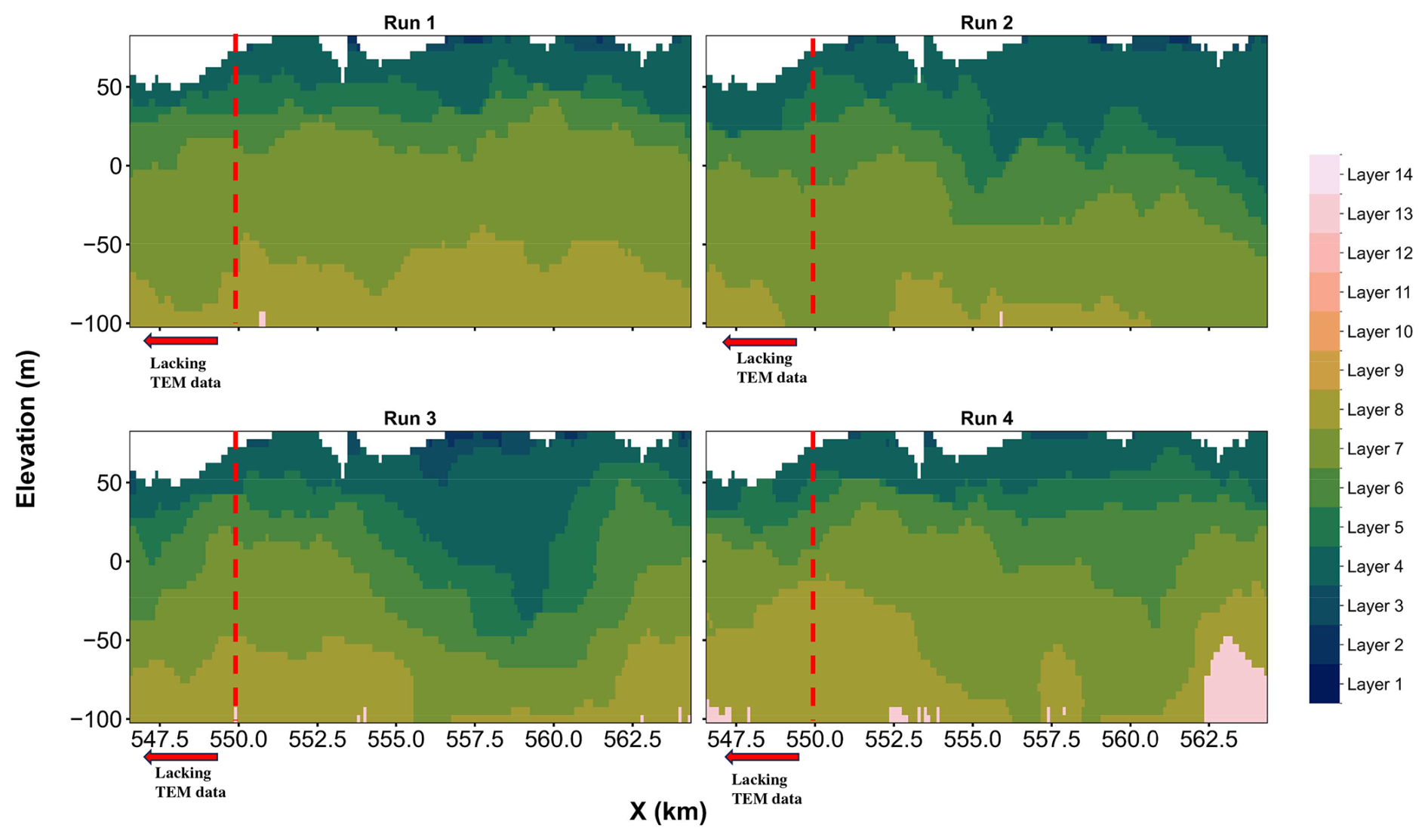
Figure A1 Four additional example realizations from MCP simulations without adding geophysical constraint (Transect of Y=6 201 300 UTM).

A1.2 Example realizations from MCP with geophysical constraint

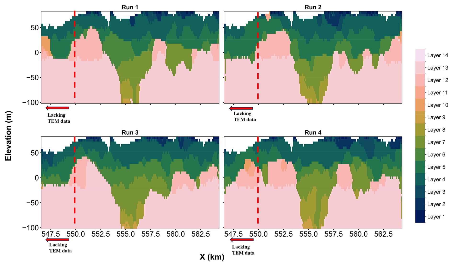
Figure A2 Four additional example realizations from MCP simulations after adding geophysical constraint (Transect of Y=6 201 300 UTM).

A2 Transect at X=553 600 UTM

A2.1 Example realizations from MCP without geophysical constraint

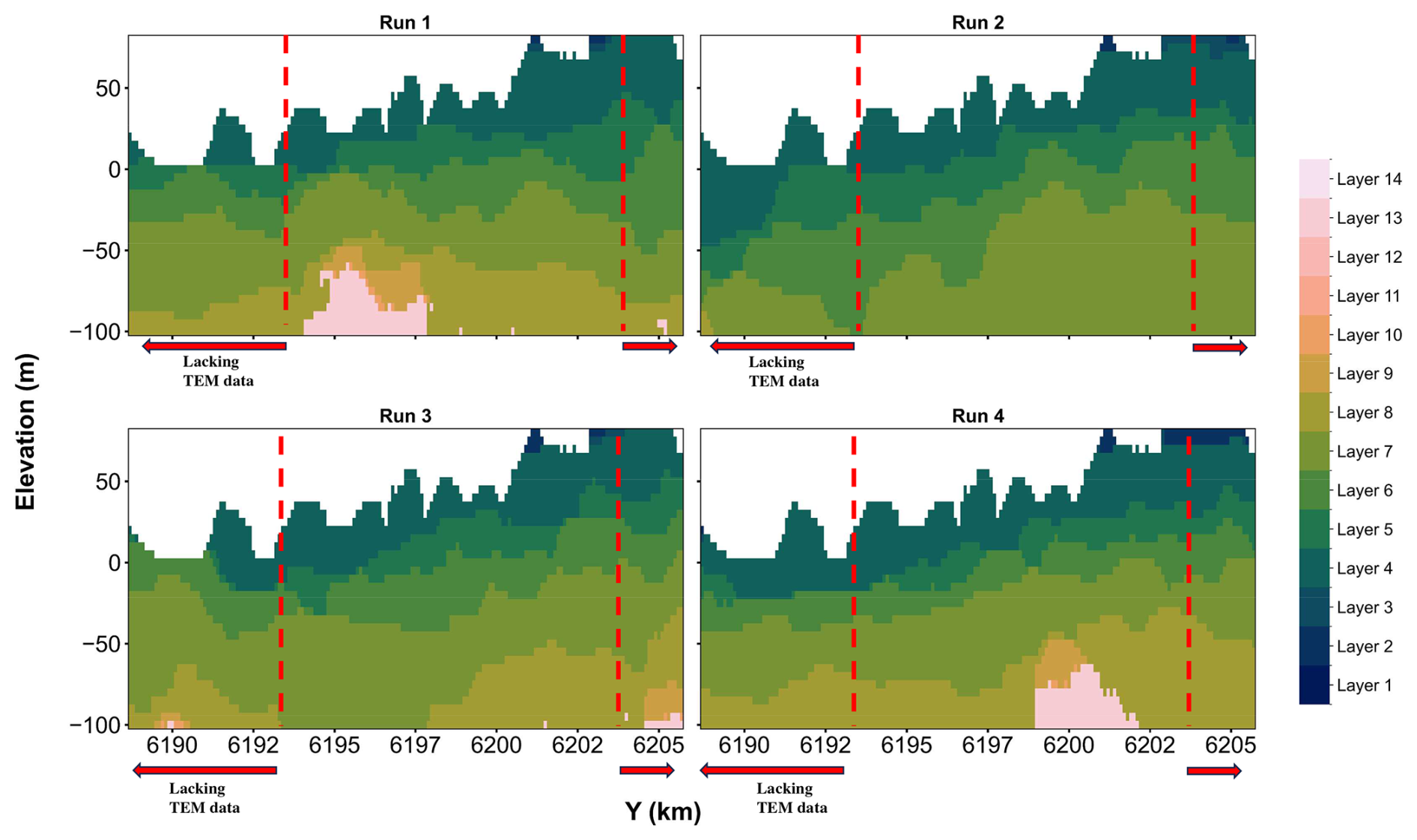
Figure A3 Four additional example realizations from MCP simulations without adding geophysical constraint (Transect of X=553 600 UTM).

A2.2 Example realizations from MCP with geophysical constraint

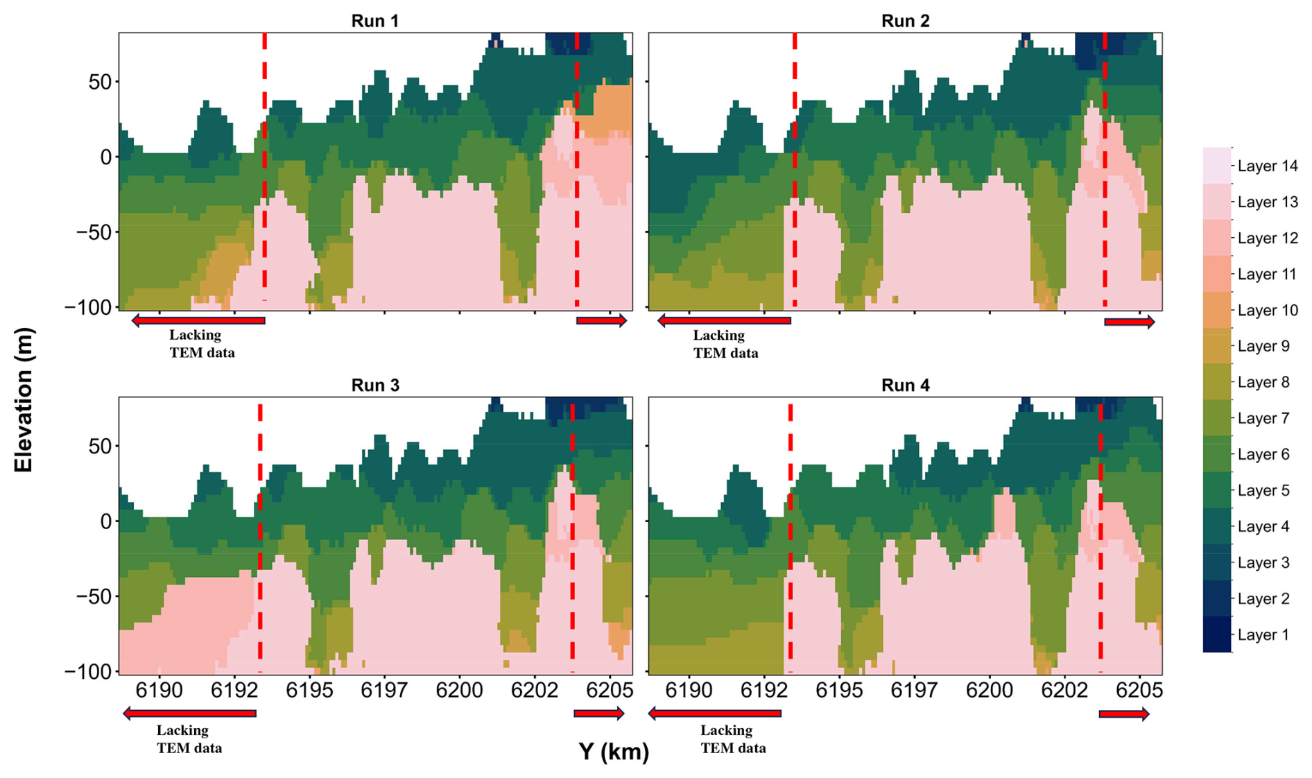
Figure A4 Four additional example realizations from MCP simulations after adding geophysical constraint (Transect of X=553 600 UTM).