Assessing the impact of Earth Observation data-driven calibration of the melting coefficient on the LISFLOOD snow module

LISFLOOD is a continental, operational hydrological model widely used in Europe. Among various hydrological processes, it simulates snowmelt using a degree-day approach, where the snowmelt coefficient is typically calibrated against discharge data. This study evaluates LISFLOOD’s current snow module and investigates the effects of a post-replacement of the snowmelt coefficient across nine European basins with varying snow influence. The parameter is calibrated using Earth Observation (EO) snow cover fraction (SCF). The outcomes illustrate the extent to which a parsimonious calibration of a single model component, intended to improve a specific module, affects hydrological model performance. To this purpose, we integrate Sentinel-2 and MODIS data to address issues related to gaps and misclassifications in snow detection over complex terrain and obtain an improved reference snow cover. Using EO SCF, we estimate a spatially distributed snowmelt coefficient, in contrast to the uniform values currently used in LISFLOOD. The coefficients are optimized by matching modelled and observed SCF, and their hydrological impacts are assessed while keeping all other model parameters unchanged. This enables us to test whether modifying only the snowmelt coefficient affects discharge performance, and whether the standard calibration adequately represents both snow dynamics and streamflow. Compared with EO SCF, the standard calibration showed biases from −1 % to 22 % and RMSE values from 20 % to 55 %. The EO-based proposed approach improved both bias and RMSE by up to 8 %. In general, the optimized coefficients did not significantly change the simulated discharge at the basin level in terms of KGE, but their application led to noticeable divergences in discharge within smaller upstream catchments. Moreover, the improved representation of snow cover led in some cases to shifts in the timing and magnitude of snowmelt and total runoff. These findings highlight the potential of integrating EO data to calibrate the snowmelt coefficient without changing other calibration parameters. This approach may offer practical advantages in situations that require accurate snow cover representation without the need for a complete re-calibration, which may be overly onerous. Nevertheless, our results indicate that standard calibration procedures already provide an acceptable representation of snow dynamics.

1 Introduction

Snow cover plays a critical role in hydrological processes, particularly in snow-fed regions where snowmelt is a dominant contributor to river runoff. In mountainous and snow-dominated basins, snowmelt can account for 40 %–95 % of annual discharge, depending on geography and climate (Viviroli et al., 2007). This makes accurate snowmelt modeling essential for flood forecasting, drought monitoring, and long-term water resource management, especially under changing climatic conditions (Barnett et al., 2005; Blöschl et al., 2017; Beniston et al., 2011).

Hydrological models are often coupled with degree-day formulations to represent snow processes (Hock, 2003). Most models calibrate snow-related parameters against streamflow observations. While effective for discharge simulation, this approach suffers from equifinality: multiple parameter sets can reproduce streamflow equally well but yield unrealistic representations of snow accumulation and melt (Beven, 2006, 2019). This problem is particularly pronounced in large-scale models, where uniform calibration across diverse catchments compounds structural uncertainties (Beven, 2012). As a result, calibration based solely on discharge is insufficient for reliable snow-related applications. Thanks to the increased availability of snow data, multi-objective calibration approaches that incorporate snow observations in addition to streamflow have been developed. In this context, several approaches have been proposed that incorporate snow data either sequentially during the calibration process (e.g., Ragettli and Pellicciotti, 2012; Kelleher et al., 2017) or simultaneously with streamflow observations (e.g., Finger et al., 2011; Pellicciotti et al., 2012; Ruelland, 2023).

Among the different types of snow observations, Earth Observation (EO) data provide an opportunity to ingest spatially distributed information over remote areas. Over the past 15 years,multi-objective calibration approaches that combine streamflow and satellite-derived snow cover have been largely explored (e.g., Franz and Karsten, 2013; Avanzi et al., 2020; Xiao et al., 2022; Zhu et al., 2024; Ruelland, 2024). Although snow cover observations do not provide volumetric information, their joint use with discharge data has been shown to improve the spatial realism of modelled processes (Finger et al., 2011). Previous studies have suggested that parsimonious calibration strategies, in which only a limited number of parameters are adjusted, may be preferable (Ruelland, 2023). In addition, direct parameter estimation against observations – rather than relying solely on standard calibration routines – has been shown to yield more realistic model representations (He et al., 2014).

Focusing on degree-day models, a key parameter governing snowmelt is the snowmelt coefficient (C_m). Standard calibration routines typically yield a lumped coefficient, thus neglecting the spatial and temporal variability induced by topography and melt processes (Pellicciotti et al., 2005). While this issue can be addressed by integrating enhanced temperature-index formulations or full energy-balance snow models, doing so substantially increases computational complexity. The integration of EO observations provides an opportunity to enhance process realism by estimating spatially varying snowmelt coefficients in a relatively straightforward manner, directly informed by observed values. Previous studies have explored the estimation of spatially distributed snowmelt parameters, for example by incorporating snow disappearance dates (Asaoka and Kominami, 2013) or by using binary snow-cover information (Gyawali and Bárdossy, 2022). However, these approaches may not fully exploit the information contained in the temporal evolution of snow cover depletion, and thus in the snow cover fraction (SCF) trends over time. For instance, Riboust et al. (2019) introduced a hysteresis-based comparison of snow cover fraction and applied an optimization criterion, but this approach was limited to elevation bands rather than fully distributed spatial units. Moreover, the resulting estimates may be constrained by the quality of the observations and forcing data (Ruelland, 2024).

Given the substantial computational effort required by multi-objective calibration, this study explores a parsimonious alternative suitable for continental-scale operational models: a post-replacement of the snowmelt coefficient (C_m). The investigated model is LISFLOOD, the distributed hydrological model underpinning Europe’s operational flood and drought monitoring systems (De Roo et al., 2000; Van Der Knijff et al., 2010; Burek et al., 2013), focusing on its temperature-index snow module. While the standard LISFLOOD setup relies on a lumped C_m constant for each sub-catchment disregarding temporal and spatial variability, our approach tests whether C_m can be estimated pixel-wise from Earth Observation snow cover fraction (EO-SCF) data after standard streamflow calibration. This approach isolates the effects of snowmelt parameterization without re-calibrating the entire model.

The pixel-based optimization minimizes the error between LISFLOOD-simulated SCF (L-SCF) and a novel, high resolution (50 m, daily) gap-filled EO-SCF (Premier et al., 2021). To facilitate this, we implement a parameterization to convert snow water equivalent (SWE) simulated by LISFLOOD to SCF (Swenson and Lawrence, 2012). This high-resolution approach represents a significant advancement over previous studies using lower-resolution products like MODIS (500 m) (Thirel et al., 2012; Pistocchi et al., 2017). Finally, we re-run LISFLOOD with the newly estimated snowmelt coefficient (EO-C_m), keeping all other settings consistent with the standard setup to specifically assess the effects of a more consistent representation of the snow module on hydrological response.

Overall, we evaluate: (i) the ability of the current LISFLOOD setup to reproduce snow and streamflow; (ii) the potential of EO-C_m to improve snow process realism; and (iii) the impact of the new, distributed EO-C_m on hydrological performance. This work provides a foundation for a future two-step calibration in LISFLOOD.

We test this approach in nine European watersheds selected to represent diverse topographical and climatic conditions, including major mountain ranges and a wide range of latitudes. These basins also feature different land cover types, from rugged mountainous terrain to flat, forested areas, offering a comprehensive foundation for evaluating the model’s performance in diverse environmental contexts. Although demonstrated here for LISFLOOD, the approach is general and transferable to other large-scale hydrological models.

2 Methods

Our methodology combines EO snow cover data with the LISFLOOD hydrological model to evaluate and improve the representation of snow processes. The workflow is illustrated in Fig. 1.

Figure 1 Workflow of the methodology.

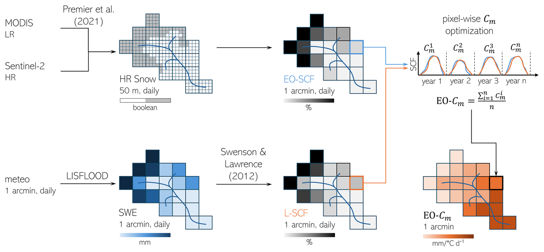
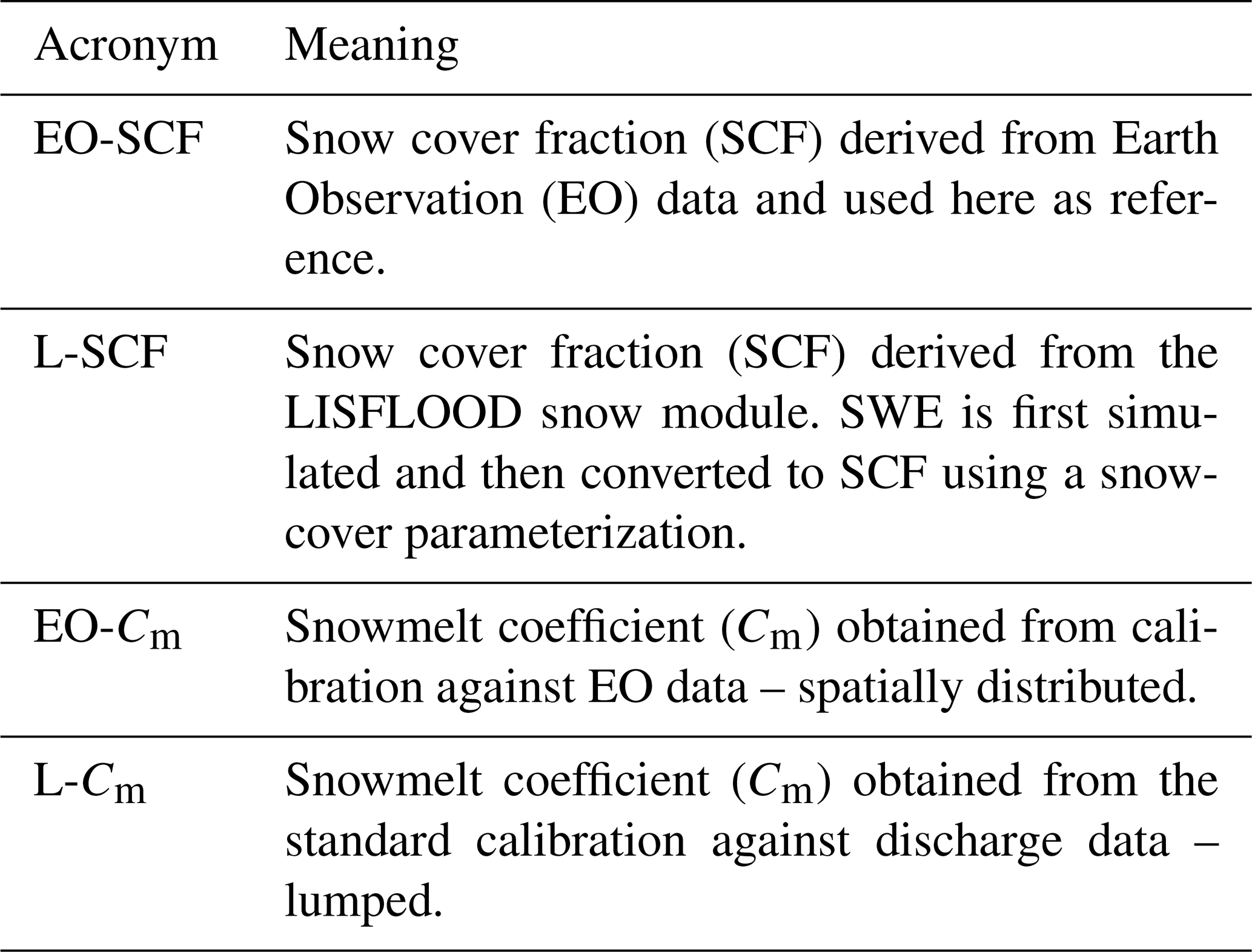
Daily high-resolution (50 m) binary snow cover data are used to derive SCF time series (hereafter EO-SCF; Sect. 2.1). In parallel, the LISFLOOD snow module (Sect. 2.2) is run to simulate SWE. A parameterization is then applied to transform SWE into modelled SCF (hereafter L-SCF; Sect. 2.3), enabling direct comparison with EO-SCF. The snowmelt coefficient (C_m) is treated as a free parameter of the snow module. We estimate C_m by minimizing the difference between L-SCF and EO-SCF through an optimization procedure (Sect. 2.4). For each year, we obtain a spatially-distributed coefficient (EO-C_m). Given the temporal stability of the obtained coefficient (see later in Sect. 4.1), a pixel-wise average over time is then computed. One season (2022/23) is excluded from calibration and used only for evaluation. In the final LISFLOOD re-run, the discharge-calibrated coefficient (L-C_m) is replaced by EO-C_m. For clarity, all acronyms used throughout the manuscript are summarized in Table 1.

Table 1 List of acronyms used in this study.

2.1 Daily Snow Cover Area Retrieval

EO optical observations have proven highly accurate for snow monitoring (e.g., Tedesco, 2015; Bormann et al., 2018), yet their applicability is limited by sensor constraints and environmental factors (Riggs et al., 2015; Engel et al., 2017). A primary challenge is the trade-off between spatial and temporal resolution. Low-resolution (LR) sensors, such as MODIS or VIIRS, provide daily estimates of snow cover fraction (SCF) but do not sample the process with the spatial detail required in complex alpine terrain (Molotch and Margulis, 2008). In contrast, high-resolution (HR) sensors, such as Sentinel-2, capture fine-scale spatial patterns but have infrequent revisit times, making them less suitable for tracking rapidly changing snow dynamics. Additionally, all optical sensors are affected by persistent cloud cover, which creates substantial data gaps–particularly in mountainous regions (Parajka and Blöschl, 2006). To our knowledge, standard operational products rely on very basic gap-filling methods as multi-temporal filters, that do not consider the spatial context.

To address these limitations, we adopt the approach of Premier et al. (2021), which integrates LR and HR optical satellite observations to produce a continuous, gap-free daily binary snow dataset (snow/snow-free) at HR (50 m). The method combines (i) LR daily SCF products (e.g., MODIS) and (ii) HR Sentinel-2 snow maps within an iterative gap-filling and downscaling framework, followed by a machine learning correction step. This framework relies on the assumption that inter-annual snow patterns are strongly influenced by local topography (elevation, slope, aspect) and meteorological conditions, resulting in recurrent spatial patterns of snow accumulation and ablation. By leveraging a long archive of HR acquisitions, the method reconstructs daily HR snow maps while correcting for known LR limitations, including errors from grain size variability, solar zenith angle, viewing geometry, and atmospheric effects. Details about the performance of the algorithm can be found in the original work.

The gap-filled HR binary snow maps are aggregated and resampled to the LISFLOOD model grid to derive daily pixel-wise SCF values, hereafter referred to as EO-SCF. Starting from HR products preserves spatial details, even after aggregation, which are crucial for accurate modeling and analysis. Specifically, using HR data enables better detection of small-scale snow patches and fractional snow cover – features often missed by LR products – thereby providing substantial improvements during the melting period, which is the main focus of this study.

A detailed description of the input datasets and a comparison with operational gap-filled products – which could provide users with faster and alternative access – is provided in Appendix A. Evaluation against other existing snow cover products highlights the key strengths of this approach, notably the availability of a fully gap-filled daily HR dataset.

2.2 The LISFLOOD Model

LISFLOOD is an open-source, spatially distributed hydrological model designed to simulate the complete water cycle in large river basins (De Roo et al., 2000; Van Der Knijff et al., 2010; Burek et al., 2013). Developed by the European Commission's Joint Research Centre (JRC) for the Copernicus Emergency Management Service (CEMS), it underpins both the European Flood Awareness System (EFAS) (JRC, 2024a; Matthews et al., 2025b) and the Global Flood Awareness System (GloFAS) (JRC, 2024b; Matthews et al., 2025a), and supports the European and Global Drought Observatories (EDO and GDO) by providing key hydrological indicators (Cammalleri et al., 2015, 2017) (see https://drought.emergency.copernicus.eu/, last access: 23 January 2026). The current EFAS and EDO setup (v5.0) operates on a 1 arcmin grid covering the European Union, the European continent, and the Mediterranean coast, while GloFAS and GDO operate globally at 3 arc-minute resolution. The model includes multiple process modules, including surface runoff, infiltration, groundwater recharge, and snow dynamics. Human influences are also represented in the model. A water abstraction module simulates withdrawals from rivers and aquifers for irrigation, livestock, domestic, and industrial uses. Reservoirs are modelled using defined conservative, normal, and flood storage limits, along with corresponding discharge rules, thereby mimicking typical operational behavior within the hydrological routing scheme. LISFLOOD can be applied at multiple scales, from large river basins to global regions, supporting flood forecasting, water resource assessments, and analyses of water demand, river regulation, land-use changes, and climate change.

2.2.1 EFAS5 Setup

In this study, we refer to the EFAS5 setup, which is forced by precipitation and temperature fields from the EMO-1 dataset (Thiemig et al., 2022). In the standard LISFLOOD calibration, 14 model parameters – including the snowmelt coefficient – are optimized to reproduce observed river discharge by using the Distributed Evolutionary Algorithms in Python (DEAP) (Fortin et al., 2012), with the modified Kling-Gupta Efficiency (KGE) (Kling et al., 2012) as the objective function. Details on the calibrated parameters and their ranges are available at: https://ec-jrc.github.io/lisflood-code/4_annex_parameters/, last access: 23 January 2026. Calibration and validation periods are constrained by the availability of observed data, with a minimum of 4 years required for calibration (https://confluence.ecmwf.int/display/CEMS/EFAS+v5.0+-+Calibration+Data, last access: 23 January 2026). The final EFAS5 evaluation is performed using the complete set of observed data, including those employed for both calibration and validation. The model assessment in this study utilizes all available observations at the outlet of each selected basin.

When multiple stations are available within a catchment, the calibration process follows a cascading approach: the basin is divided into sub-catchments, and each is calibrated sequentially from upstream to downstream. Parameters for ungauged basins are estimated using a regionalization approach (Beck et al., 2016), while coastal and endorheic catchments (area < 150 km²) use default values. Each parameter is assigned a uniform value across all pixels within a sub-catchment. The snowmelt coefficient obtained through this standard procedure is referred to as L-C_m.

In this study, we recalibrate only the snowmelt coefficient, integrated in the snow module of the model, against EO data (see Sect. 2.4). The remaining 13 parameters are kept unchanged, following the EFAS5 setup. This approach has been described as “sequential” in previous studies (e.g. Franz and Karsten, 2013; Ruelland, 2024), with the difference that the remaining parameters were calibrated after the calibration of the snow-related ones. In this study, by holding these parameters constant and re-running LISFLOOD with the updated snowmelt coefficient, we isolate the direct impact of the EO-based calibration on simulated river discharge. This approach allows us to determine whether modifying the snowmelt coefficient alone produces significant effects on discharge, and to test whether the standard LISFLOOD calibration sufficiently captures snow dynamics and streamflow. A detailed explanation of the methodology and criteria used to evaluate the LISFLOOD model outputs is provided in Sect. 4.4.

2.2.2 LISFLOOD Snow Module

Since the snowmelt coefficient is the focus of this study, we provide a detailed description of the snow module. LISFLOOD simulates snowmelt using a temperature-index approach – specifically, a degree-day model that also accounts for enhanced melt during rainfall events (Speers and Versteeg, 1982).

The SWE is computed by accounting for both accumulation and melt processes. Total precipitation is partitioned in rainfall (P_rain) or solid precipitation (P_snow) based on a temperature threshold that is set to 1 °C. Two melt processes are modelled: snowmelt (SM) and icemelt (IM). All the variables listed above are expressed in mm.

$$\begin{array}{}\text{(1)}& {\mathrm{SWE}}_t=max\left(\mathrm{0},{\mathrm{SWE}}_{t-\mathrm{1}}+P_{\mathrm{snow}}-\mathrm{SM}-\mathrm{IM}\right)\end{array}$$

Snowmelt (SM) occurs when the average temperature (T_avg [°C]) exceeds a threshold (T_m[°C]), which is set to 1 °C. The rate of melt is controlled by the snowmelt coefficient, which is partitioned into a fixed term (C_m [mm (°C d)⁻¹]) and a seasonal term (C_seas [mm (°C d)⁻¹]). The focus of this study is the calibration of that fixed term (C_m). The seasonal term (C_seas) allows for a sinusoidal variation of the snowmelt coefficient of ±0.5 mm (°C d)⁻¹ depending on the day of the year (doy). To account for increased snowmelt under rain, the snowmelt coefficient is further increased by 1 % per mm of rainfall (P_rain).

$$\begin{array}{}\text{(2)}& {\displaystyle }\mathrm{SM}=\left\{\begin{array}{ll}(C_{\mathrm{m}}+C_{\mathrm{seas}})\cdot (\mathrm{1}+\mathrm{0.01}\cdot P_{\mathrm{rain}})\cdot (T_{\mathrm{avg}}-T_{\mathrm{m}})\cdot \mathrm{\Delta }t& \mathrm{if}{T}_{\mathrm{avg}}>T_{\mathrm{m}}\\ \mathrm{0}& \mathrm{if}{T}_{\mathrm{avg}}\le T_{\mathrm{m}}\end{array}\right.\text{(3)}& {\displaystyle }{C}_{\mathrm{seas}}={\displaystyle \frac{\mathrm{1}}{\mathrm{2}}}\sin \left({\displaystyle \frac{\mathrm{2}\mathit{\pi }}{\mathrm{365.25}}}(\mathrm{doy}-\mathrm{81})\right)\end{array}$$

Icemelt (IM) represents the runoff from glacier melt at high altitudes, where temperature rarely exceeds the melting threshold (T_m). It is constrained to the summer season – from 13 June (start) to 13 September (end) in the Northern Hemisphere. The process is controlled by the seasonally-varying icemelt coefficient (C_im), which has a maximum value of 7 mm (°C d)⁻¹.

$$\begin{array}{}\text{(4)}& {\displaystyle }\mathrm{IM}=max\left(\mathrm{0},C_{\mathrm{im}}\cdot T_{\mathrm{avg}}\cdot \mathrm{\Delta }t\right)\text{(5)}& {\displaystyle }{C}_{\mathrm{im}}=\left\{\begin{array}{ll}\mathrm{7}\cdot \sin (\frac{\mathrm{4}\mathit{\pi }}{\mathrm{365.25}}\cdot (\mathrm{doy}-\mathrm{start}\left)\right)& \mathrm{if}\mathrm{start}<\mathrm{doy}<\mathrm{end}\\ \mathrm{0}& \mathrm{else}\end{array}\right.\end{array}$$

Due to the often coarse spatial resolution in LISFLOOD, the elevation differences within a pixel can be significant, which in turn affects snow processes. To overcome this limitation, LISFLOOD subdivides each pixel into three elevation zones. Snow accumulation and ablation are simulated separately within each zone, and the results are then aggregated to obtain the pixel-level SWE. A normal distribution is applied to the digital elevation model from the 90 m Multi-Error-Removed Improved-Terrain (MERIT) (Yamazaki et al., 2017) to divide the pixel in three elevations zones of equal area. The average temperature is corrected for the upper and lower elevation zones using a fixed lapse rate of 0.0065 °C m⁻¹.

For more details, the model code and documentation are available at https://ec-jrc.github.io/lisflood-model/2_04_stdLISFLOOD_snowmelt/ (last access: 23 January 2026).

2.3 Snow Cover Parametrization

To compare LISFLOOD’s SWE output with EO-SCF, SWE must be converted into snow cover fraction (SCF). This conversion requires a parametrization that accounts for variations in snow depth and density within a pixel. Due to substantial intra-pixel variability, the relationship is influenced by factors such as topography and land cover (Roesch et al., 2001). Several parameterizations have been proposed in the literature (e.g., Liston, 2004; Niu and Yang, 2007; Helbig et al., 2015; Pimentel et al., 2017; Lee et al., 2024). In this study, we adopt two approaches that balance model complexity with data availability. The first, proposed by Swenson and Lawrence (2012) and implemented in the Community Land Model (CLM), is relatively sophisticated. The second, introduced by Zaitchik and Rodell (2009), is a simpler empirical method requiring fewer inputs but has been shown to provide consistent results. For brevity, and given their similar performance, details and results from the second approach are provided in Appendix B.

Swenson and Lawrence (2012) differentiates the accumulation and ablation periods. For the accumulation, the SCF after a precipitation event can be interpreted probabilistically. In a simple linear formulation, the probability of a pixel to be snow covered or the SCF is given by the following formula:

$$\begin{array}{}\text{(6)}& \mathrm{SCF}=min(\mathrm{1},k_{\mathrm{accum}}\cdot \mathrm{SWE}),\end{array}$$

where k_accum [1 mm⁻¹] is a scaling parameter that relates SWE to SCF. Accordingly, the probability that a pixel remains snow-free is 1−SCF. For multiple independent snowfall events, the cumulative probability that a pixel remains snow-free is the product of the individual probabilities. Therefore, after N+1 events, the cumulative SCF is

$$\begin{array}{}\text{(7)}& {\mathrm{SCF}}_{N+\mathrm{1}}=\mathrm{1}-\prod _{i=\mathrm{0}}^N(\mathrm{1}-{\mathrm{SCF}}_i).\end{array}$$

A more refined, probabilistic formulation for accumulation uses a hyperbolic tangent function, which ensures that SCF asymptotically approaches 1 as SWE increases, to update SCF after each event:

$$\begin{array}{}\text{(8)}& {\mathrm{SCF}}^{n+\mathrm{1}}=\mathrm{1}-\left[\right(\mathrm{1}-\tanh \left(k_{\mathrm{accum}}\mathrm{\Delta }\mathrm{SWE}\right)\left)\right(\mathrm{1}-{\mathrm{SCF}}^n\left)\right],\end{array}$$

where ΔSWE is the amount of new SWE in mm. Although many state-of-the-art models assume a constant value for k_accum equal to 0.1, it likely varies pixel-wise due to topographic differences. The parameter k_accum can be estimated by measuring SCF and ΔSWE during precipitation events over an initially snow-free area, as suggested by Swenson and Lawrence (2012). To identify such conditions, we selected the first day on which both EO-SCF observations and LISFLOOD SWE are greater than 0 (snow presence). Equation (8) is then inverted to obtain an estimated value of k_accum. The parameter is constrained to a maximum of 0.5, consistent with what reported in the original study. For pixels that never exhibit snow, the default value is retained. This procedure was repeated for all calibration seasons, and the final pixel-wise value of k_accum was taken as the average over time. The obtained parameters are reported in Appendix B in Fig. B1.

For the melting period, Swenson and Lawrence (2012) relate SCF to the dimensionless snow water equivalent scaled by the maximum SWE (SWE_max) through the following empirical equation:

$$\begin{array}{}\text{(9)}& \mathrm{SCF}=\mathrm{1}-[{\displaystyle \frac{\mathrm{1}}{\mathit{\pi }}}\arccos \left(\mathrm{2}{\displaystyle \frac{\mathrm{SWE}}{{\mathrm{SWE}}_{\text{max}}}}-\mathrm{1}\right){]}^{N_{\mathrm{melt}}}\end{array}$$

where N_melt is a parameter that depends on the topographic variability within the grid cell. It is calculated as follows:

$$\begin{array}{}\text{(10)}& N_{\mathrm{melt}}={\displaystyle \frac{\mathrm{200}}{max(\mathrm{10},{\mathit{\sigma }}_{\mathrm{topo}})}}\end{array}$$

with σ_topo being standard deviation of the elevation within a grid cell calculated from the MERIT DEM with a spatial resolution of 90 m (Yamazaki et al., 2017). When an accumulation follows a melting event, SWE_max needs to be updated to re-define a consistent depletion curve. This is done by inverting Eq. (9) and using the following equation:

$$\begin{array}{}\text{(11)}& {\mathrm{SWE}}_{\text{max}}={\displaystyle \frac{\mathrm{2}\mathrm{SWE}}{\cos \left(\mathit{\pi }\right(\mathrm{1}-\mathrm{SCF}{)}^{\mathrm{1}/N_{\mathrm{melt}}})+\mathrm{1}}}\end{array}$$

Note that Eq. (11) would be circular with respect to Eq. (9); however, after a new snowfall event, SWE_max is updated such that the previous SCF (prior to snowfall) is preserved along the depletion curve. In other words, SWE_max refers to SCF(t−1). For more details, refer to the original code at https://github.com/ESCOMP/CTSM/blob/master/src/biogeophys/SnowCoverFractionSwensonLawrence2012Mod.F90 (last access: 23 January 2026), which implements the snow cover fraction parameterization by Swenson and Lawrence (2012).

2.4 Snowmelt Coefficient Estimation from EO Data

The snowmelt coefficient is estimated by solving an optimization problem that minimizes the error between L-SCF and EO-SCF. This procedure aims to align model outputs with observations, thereby increasing the realism of the simulation results. We remark that L-SCF is derived from modelled SWE using Eq. (1) and the parametrization defined in Eqs. (8) and (9), with C_m treated as a free parameter in this optimization phase. Specifically, we minimize the mean squared error (MSE) over time to identify the optimal coefficient that produces the smallest discrepancy. Accordingly, the following minimization problem is solved for each pixel to obtain the EO-based snowmelt coefficient:

$$\begin{array}{}\text{(12)}& \mathrm{\text{EO-}}{C}_{\mathrm{m}}=\arg \underset{C_{\mathrm{m}}}{min}\sum _{t\in {\mathcal{T}}_{\mathrm{hy}}}{\left(\mathrm{L}-\mathrm{SCF}(t,C_{\mathrm{m}})-\text{EO-SCF}\left(t\right)\right)}^{\mathrm{2}}\end{array}$$

The optimization is performed on a pixel-wise basis over all time steps within a given hydrological year 𝒯_hy to obtain a single, time-invariant coefficient. To solve this optimization problem, we utilize the L-BFGS-B algorithm – a limited memory quasi-Newton, gradient-based optimization algorithm – provided in the SciPy library (Virtanen et al., 2020). Estimated values are constrained between 0.5 and 10, as values outside this range lack physical meaning and may result from errors, such as having too few days to perform a reliable optimization (e.g., ephemeral snow at low altitudes). Specifically, according to Eq. (2), lower values of C_m would result in negative melting, which is not physically realistic. Subsequently, a mean value for each pixel is calculated using data from five seasons (2017/22) while one (2022/23) is used exclusively for a further independent assessment of the results. For pixels where the coefficient could not be estimated – such as those without snow during the year or where pixels were masked out due to the presence of water bodies – L-C_m is retained.

2.5 Assessment of the Results

The obtained EO-C_m is first evaluated qualitatively against L-C_m. A correlation analysis is also performed against selected topographic, geographic, and land cover features. For a quantitative assessment, we compare the resulting snow-covered area (SCA), defined as the percentage of the basin covered by snow. To do this, SWE is simulated using the LISFLOOD snow module (Eq. 2) with both L-C_m and EO-C_m. The simulated SWE is then converted to SCF (see Sect. 2.3) and aggregated to the basin level to obtain SCA. The SCA obtained using L-C_m is denoted as L-SCA L-C_m, while that obtained using EO-C_m is denoted as L-SCA EO-C_m. These model-based estimates are then compared against EO-SCA, derived from EO-SCF, which serves as the benchmark. The results are reported in Sect. 4.1.

We also evaluate improvements at the pixel scale by computing metrics for SCF, using EO-SCF as the benchmark. Specifically, we calculate bias, root mean squared error (RMSE), and correlation between L-SCF (using both L-C_m and EO-C_m) and EO-SCF. Metrics are first computed per pixel over time and then averaged spatially across the basin. To focus on the model’s ability to detect snow, we exclude pixels where both modelled and observed SCF are zero (i.e., snow-free conditions). Including such pixels would artificially inflate performance metrics, particularly during periods when large portions of the basin are snow-free, thereby biasing the results. An analysis of the correlation with the errors versus physiographic and climatic features is also performed, together with an evaluation of the seasonal error trends. SCA results are reported in Sect. 4.2.

A SWE intercomparison is performed for basins where a reference dataset is available. To complete the assessment, we evaluate how the hydrological response changes when using EO-C_m. Specifically, we replace L-C_m with EO-C_m and run the LISFLOOD model from 1990 to 2023, including two warm-up years (1990–1991). The remaining 13 model parameters are kept unchanged, allowing us to isolate the impact of C_m on river discharge and assess whether the current EFAS5 setup can realistically capture snow accumulation and melt dynamics in the selected catchments. These results are reported in Sect. 4.3.

We compare the mean annual hydrographs of the two simulations for periods with observations to check if changes in SWE and snowmelt are reflected in the simulated discharge. In addition, we calculate the Kling-Gupta Efficiency (KGE) both over the entire period and aggregated by month, using daily simulated and observed river discharge data. This allows us to evaluate the overall performance of the simulations as well as their performance across different sections of the annual hydrograph, with particular attention to potential increases or decreases in performance during the snowmelt season. Finally we evaluate the spatial similarity of river discharge at pixel level to identify main difference between EO-C_m and L-C_m simulations upstream of the discharge station. The analysis focuses on upstream catchment areas larger than 100 km² to exclude very small headwater sections that may introduce noise in spatial comparisons. To do so, we extract daily river discharge time series from both model outputs and apply min-max normalization for each grid cell, standardizing discharge values across different magnitudes and catchments. We then compute the Euclidean distance between the normalized discharge values of the two models at each grid cell, quantifying the absolute dissimilarity in flow dynamics over time. The Normalized Euclidean Distance (NED) values range from 0 to infinity, where a value of 0 indicates that the two time series are identical or highly similar, and larger values signify greater dissimilarity between the time series. These results are reported in Sect. 4.4.

3 Test sites

In this study, we analyze nine snow-dominated hydrological basins across Europe, located in Italy, Switzerland, Austria, Germany, France, Spain, Slovakia, and Sweden. These basins were selected for their strong snow influence on hydrological processes, with snow persisting for a significant portion of the year. Representing a range of geographical contexts, the basins include mountainous regions such as the Alps and Pyrenees, as well as flatter terrains in Scandinavia. They also exhibit diverse land cover, including varying proportions of forested areas, which influence snow accumulation and melt.

For example, Mörrumsån (Sweden) and Laborec (Slovakia) are relatively flat with brief, intermittent snow periods, with Laborec also having significant forest cover. Umeälven (Sweden), though similarly flat, experiences prolonged snow cover lasting several months due to its high latitude. In contrast, the remaining basins exhibit a more typical alpine snowpack. Some basins (Adige, Alpenrhein, Arve, and Salzach) contain glaciers, though glacier-covered areas are generally small – less than 1 % of the total area (approximately 0.9 % for Adige and Salzach, 0.6 % for Alpenrhein) – with the exception of Arve, where glacierized areas account for about 5 % of the basin. Two basins in Spain, Guadalfeo and Gállego, are strongly influenced by anthropogenic activities, providing an opportunity to assess model performance under different basin characteristics.

To further explore methodological differences, seven catchments were originally calibrated against observed river discharge, while two – Guadalfeo and Adige – were parameterized using the regionalization approach (see Sect. 2.2.1). For these two basins, observed river discharge data were obtained from the respective authorities, enabling the evaluation of LISFLOOD performance.

Key information on these basins is presented in Table 2 and Fig. 2. Due to the coarse model resolution, basin hypsometry is not accurately represented; for clarity, Table 2 reports the lower and upper bounds of elevation ranges used in the model, based on the three elevation zones described in Sect. 2.2.2.

Table 2 Overview of the nine hydrological catchments selected in this study, including their respective countries, area, and elevation information. The mean elevations reported here refer to the elevation from the MERIT DEM aggregated at the model resolution of 1 arcmin. Maximum and minimum elevations are calculated considering σ_topo, thus representing the minimum and maximum elevations modelled.

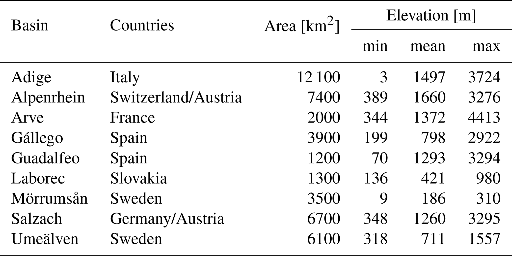
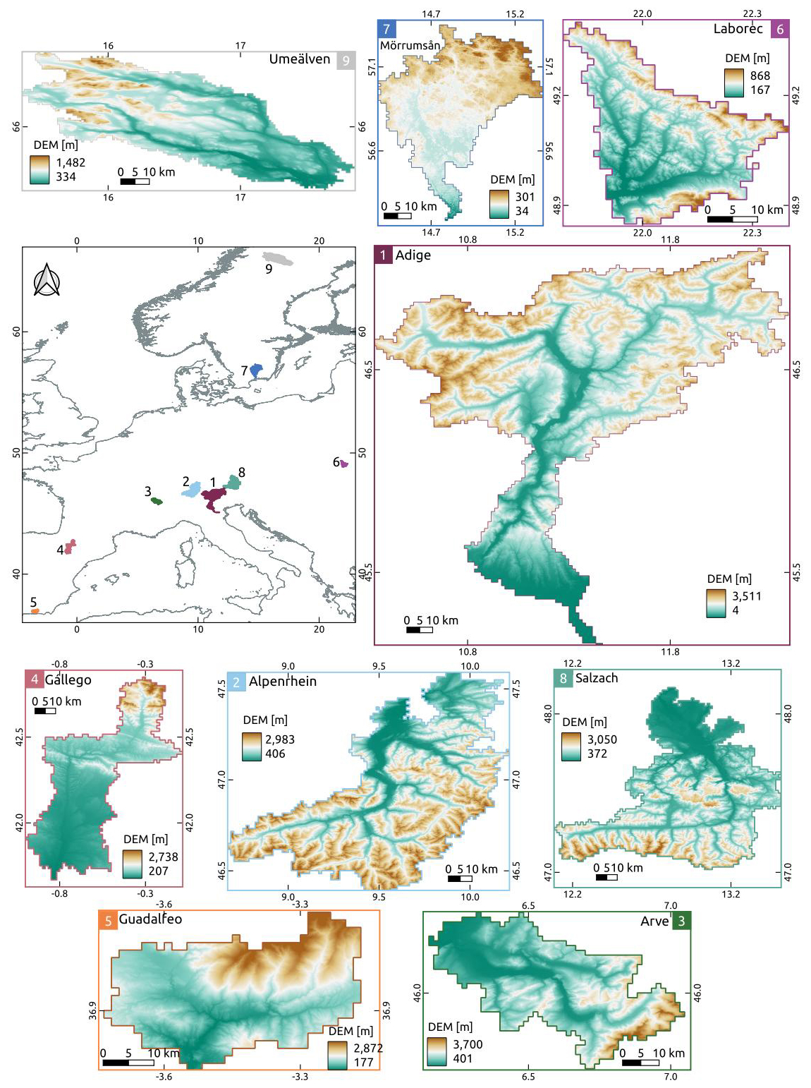
Figure 2 Overview of the nine hydrological basins chosen for this study: Adige (Italy), Alpenrhein (Switzerland/Austria), Arve (France), Gállego and Guadalfeo (Spain), Laborec (Slovakia), Mörrumsån (Sweden), Salzach (Germany/Austria) and Umeälven (Sweden). The elevations reported here (and hence the color bar ranges) refer to the MERIT DEM aggregated at the model resolution of 1 arcmin.

The EO dataset spans six hydrological years, from 1 October 2017 to 30 September 2023, corresponding to the period with maximum availability of Sentinel-2 data (both Sentinel-2A and Sentinel-2B). The last season 2022/23 is not used for the snowmelt coefficient calculation, but it is used exclusively for an independent assessment of the results. The LISFLOOD outputs were evaluated by running the model from 1992 to 2023 (see Sect. 4.4). The analysis uses the model grid with a spatial resolution of 1 arcmin (ranging from ≈ 1.48 km for the Guadalfeo to ≈ 0.75 km for the Umeälven), as described in Sect. 2.2.

4 Results

4.1 Snowmelt Coefficient Calibration

In this section, we present the snowmelt coefficients (C_m) obtained by calibrating against EO data (EO-C_m – see Fig. 4), as described in Sect. 2.4, and compare them qualitatively with the coefficients obtained from the EFAS5 calibration (L-C_m – see Fig. 3), as described in Sect. 2.2.1. L-C_m are lumped at the sub-catchment scale within the major basin, with sub-catchments defined according to the availability of streamflow data for calibration, as explained in Sect. 2.2.1. The corresponding histograms are also shown in the figures. Missing values (white areas) indicate masked regions, such as water bodies or pixels that did not experience snow during the analyzed period.

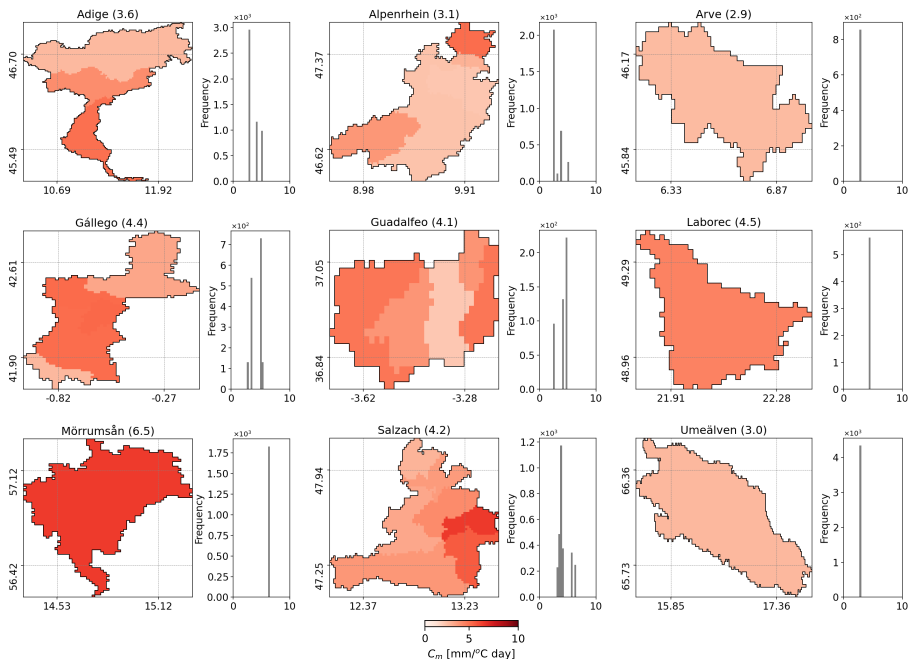
Figure 3 Snowmelt coefficients resulting from the standard hydrological calibration (L-C_m) for the nine selected basins. The corresponding histograms are also included. Missing values (in white) correspond to masked areas, such as water bodies, or pixels that never experienced snow for the analysed period. Average values are reported within brackets.

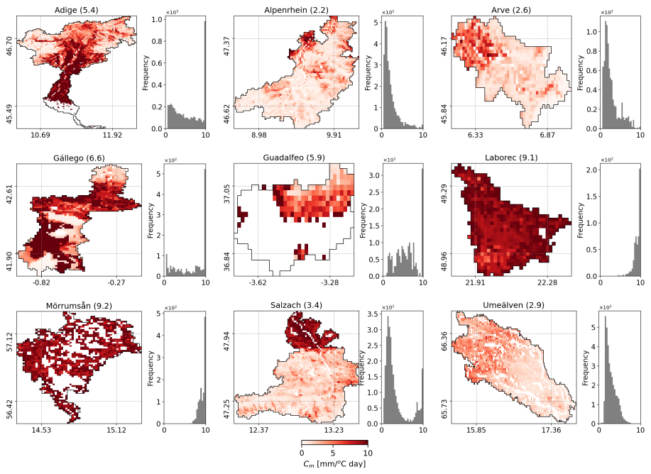
Figure 4 Snowmelt coefficients resulting from optimization based calibration against earth observation SCF (EO-C_m) for the nine selected basins. The corresponding histograms are also included. Missing values (in white) correspond to masked areas, such as water bodies, or pixels that never experienced snow for the analysed period. Average values are reported within brackets.

Notable differences are observed, as L-C_m represents a lumped coefficient, whereas EO-C_m is spatially distributed. EO-C_m exhibits very high values in basins or areas with ephemeral snow. Additionally, the parameter range in the standard LISFLOOD calibration (2.5–6.5) is narrower than in the EO-based calibration. The wider range in EO-C_m allows us to explore the potential of the new calibration to compensate for erroneous precipitation inputs and better represent the snowmelt phase (see next section). It is interesting to note that the coefficient EO-C_m assumes a value of 10 in those basins, or parts of basins, that exhibit ephemeral or short snow-cover periods, such as the Laborec and Mörrumsån, as well as the lower Adige. This value likely indicates a non-ideal optimization, possibly due to fluctuations in snow cover. We also evaluated the stability of this coefficient across different seasons. For brevity, results are reported only for the Adige River basin in Fig. 5. The figure shows that the coefficient is quite stable over years, confirming our choice of considering a temporal average.

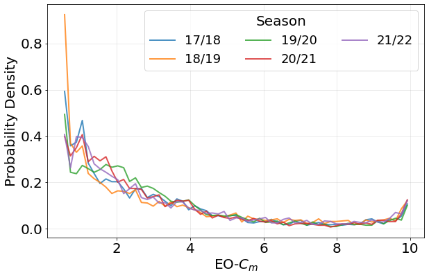
Figure 5 Probability density of the EO snowmelt coefficient for the Adige basin during the calibration season. Values of 10 are excluded for better visualization.

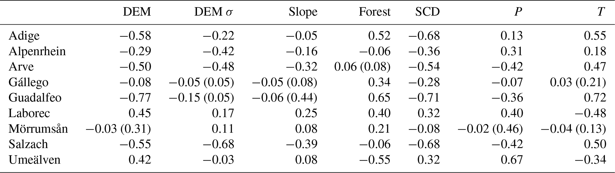
To explore whether the spatialized snowmelt coefficient calibrated at the pixel scale captures meaningful patterns, we conducted a correlation analysis with topographic, geographic, and land cover features. The motivation was that such relationships could eventually support parameterizing snowmelt based on spatial characteristics alone, thereby reducing reliance on EO data, which are often labor-intensive to process. Table 3 reports the Pearson correlation coefficients between EO-C_m and several variables: elevation (DEM), elevation variability (DEM σ), slope, forest cover, mean snow cover duration (SCD), as well as mean precipitation (P) and temperature (T), averaged over the six analyzed hydrological seasons. However, the results indicate that no strong correlations emerge from this analysis. The most influential feature appears to be elevation, which exhibits a negative correlation in the Adige, Arve, Salzach, and Guadalfeo river basins. This indicates that lower values of EO-C_m are estimated for higher elevations, meaning snow persists longer at higher elevations, as expected. For the Laborec and Umeälven basins, which are relatively flat, the correlation with elevation becomes positive. The correlation with mean snow cover duration also aligns with the findings for elevation, confirming that snow lasts longer at higher elevations. The observed correlation, together with the temporal stability of the snowmelt coefficient, may also suggest a systematic elevation-dependent bias in the precipitation forcing.

Table 3 Pearson correlation coefficients between the EO-C_m and topographical, land cover and meteorological features. The p-values are reported within brackets only if >0.05, i.e., when the results are not statistically significant.

4.2 Snow Cover Evaluation

To assess how well the standard multi-parameter calibration of streamflow captures snow dynamics and to quantify the improvements of an independently calibrated C_m, we conducted a comparative evaluation of the snow cover area (SCA). Specifically, we ran the LISFLOOD snow module using two different snowmelt coefficients: the standard, lumped value (L-C_m) and the new spatially-distributed value (EO-C_m). This produced two distinct model-derived SCA estimates (L-SCA), which were then compared against the observed SCA (EO-SCA). Note that, since the conversion from SWE to SCA is performed through a parameterized approach that relies on the parameter k_accum (see Sect. 2.3), which is derived from EO-based SCF, the two SCA estimates compared in this evaluation are not fully independent variables.

In Fig. 6, the SCA trends with the two C_m are reported. These results offer a quick overview of the performances at basin level. Furthermore, to assess improvements at the pixel-scale we report the metrics for SCF, using EO-SCF as the benchmark. These are computed per pixel along the temporal dimension and then averaged spatially. To specifically assess the model's ability to detect snow cover, we exclude pixels where both the target and reference SCF are 0 (snow-free). While including these pixels would lead to better performances, the results might be biased especially when a large portion of the basin is snow-free.

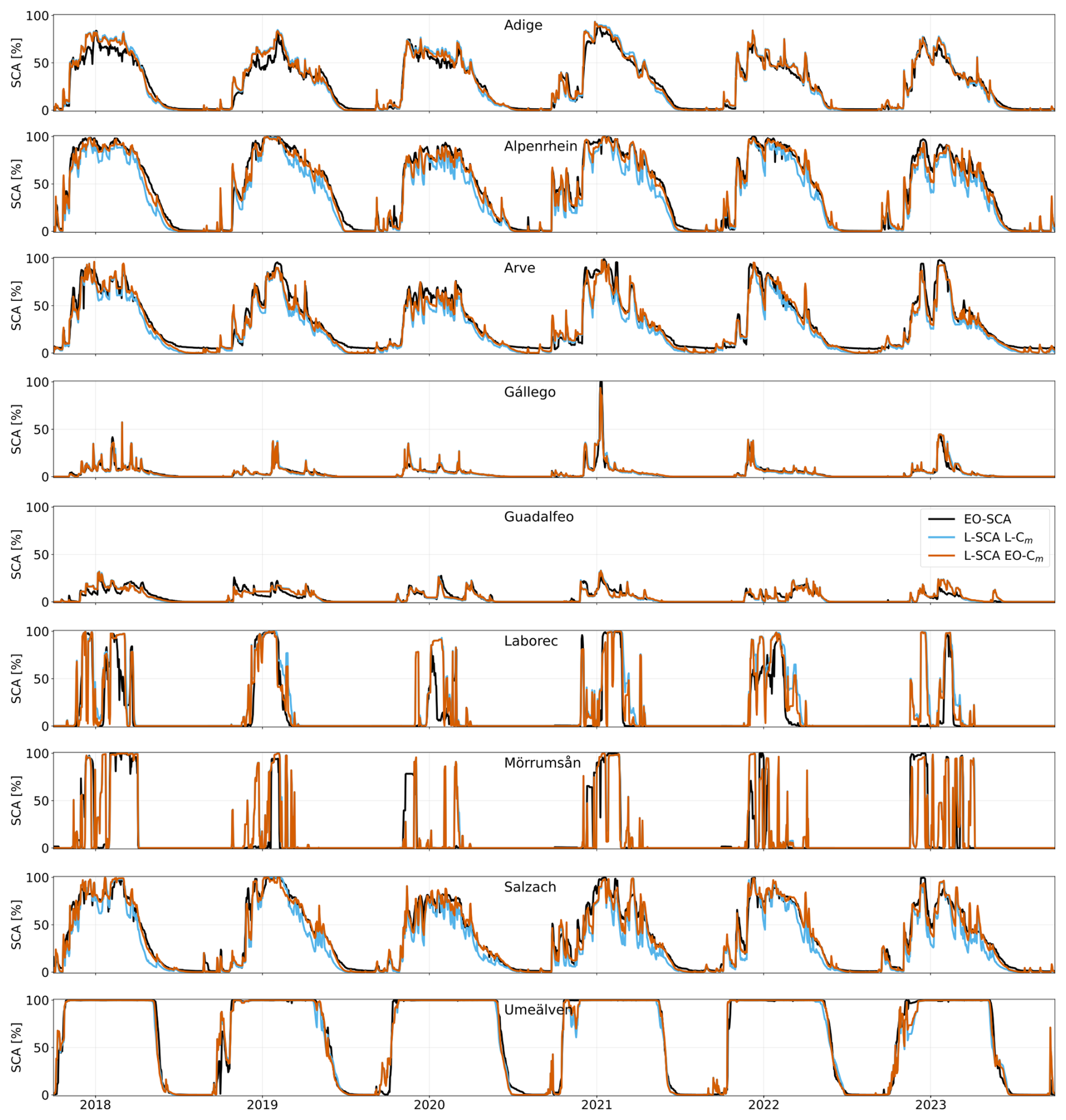
Figure 6 SCA trends for the nine river basins. In black, the observed EO-SCA, in cyan the LISFLOOD simulated SCA using the standard EFAS5 snowmelt coefficient (L-C_m), and in orange the LISFLOOD simulated SCA using the EO-optimized coefficient (EO-C_m).

In Table 4, we present the average metrics calculated across all analysed hydrological years for brevity. Similar metrics with a different SCF parametrization are reported in Table B1. Detailed metrics for each individual season are provided in Fig. 7.

Table 4 Evaluation of LISFLOOD SCF in terms of BIAS, RMSE, and correlation using the EO-SCF as benchmark. The standard EFAS5 snowmelt coefficient (L-C_m) and the EO-optimized coefficient (EO-C_m) were utilized. Pixels where both the target and reference SCF are snow-free are excluded from the analysis.

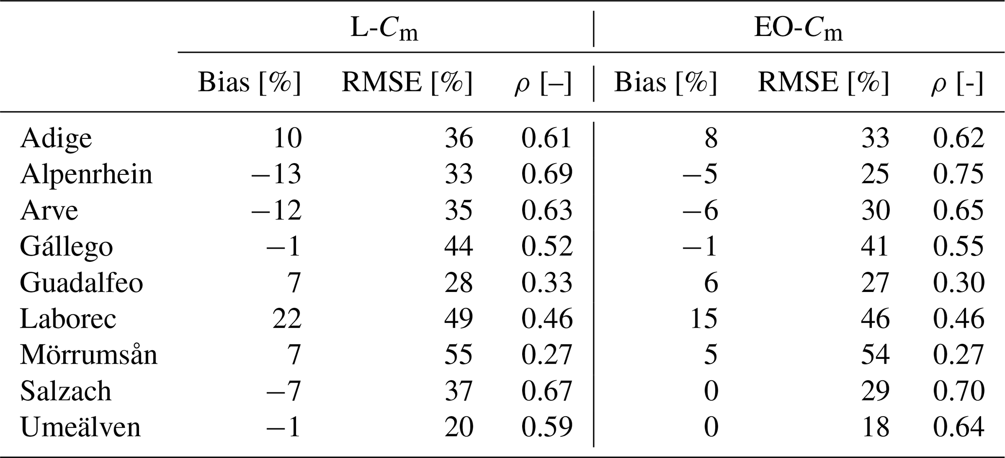
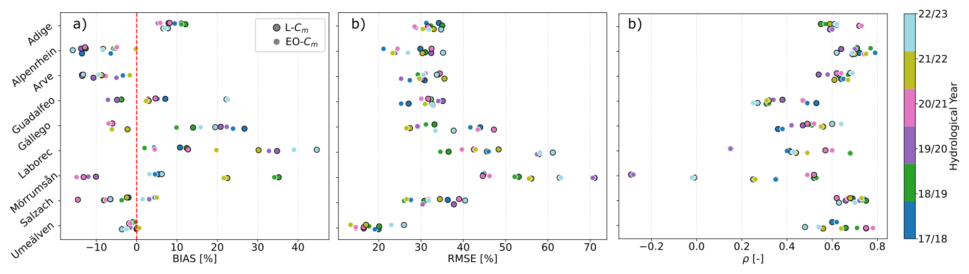
Figure 7 Evaluation of LISFLOOD SCF in terms of BIAS (a), RMSE (b), and correlation (c) using the EO-SCF as benchmark for all the basins and for each season. The standard EFAS5 snowmelt coefficient (L-C_m) and the EO-optimized coefficient (EO-C_m) were utilized. Note that season 2022/23 was used exclusively for evaluation.

Due to variations in the size and location of these basins, the SCA varies significantly and exhibits seasonal fluctuations influenced by how wet or dry the year was. For example, while most basins reach nearly 100 % snow cover at least briefly, others, such as Gállego and Guadalfeo, show very little snow cover. A generally good agreement can be observed between EO and LISFLOOD SCA, even with the EFAS5 calibration (L-C_m). However, important differences are evident in certain basins, including the Adige, Laborec, and Mörrumsån. In the Adige river basin, the LISFLOOD model shows a consistently larger SCA compared to satellite observations. These discrepancies, particularly noticeable during accumulation phases, such as in the 2020/21 season, may stem from an overestimation of snowfall and, consequently, precipitation fields over the basin, or from an inaccurate partition of solid/liquid precipitation. Despite these differences in magnitude, the timing of SCA variations appears to align well between the two datasets. Interestingly, the Arve basin shows that SCA remains above zero even during summer, as some pixels are either persistently snow-covered or correspond to glacierized areas. However, since LISFLOOD does not explicitly represent glaciers, these pixels are not simulated as permanently snow-covered in the model, thus resulting in lower SCA. On the other hand, the differences observed in the Laborec and Mörrumsån basins are more likely attributable to challenges in snow detection by the satellite. These include prolonged periods of missing acquisitions due to cloud cover, combined with ephemeral snowfalls in flat areas, as is the case in Mörrumsån. Additionally, significant forest coverage, particularly in the Laborec basin, further complicates accurate snow detection.

Overall, both the standard EFAS5 calibration and the EO-based optimization of the snow module yield satisfactory results at the basin scale. However, important differences are highlighted when considering SCF (Table 4). Before dedicated EO-based calibration, the agreement is acceptable, with the highest bias observed at approximately 20 % for the Laborec basin but with generally moderate correlation. The highest root mean square error (RMSE) values are observed for Mörrumsån and Laborec, due to the reasons previously discussed. Additionally, Gállego also exhibits notable discrepancies, likely because most pixels remain snow-covered for only short periods complicating the analysis. The computed metrics indicate that, in general, the optimization (EO-C_m) improves bias, RMSE, and correlation, except for a slight increase in bias for Gállego. As shown in Fig. 7, these trends generally persist across individual seasons, with a few exceptions. Additionally, for the year not used in coefficient calibration (2022/23), EO-C_m still demonstrates an overall improvement in performance especially in reducing the bias and RMSE and increasing the correlation. However, the remaining errors stem from the fact that the new coefficient enhances SCF during the melting season only, while errors persist during the accumulation season. Moreover, the figure shows that the Alpine basins (Adige, Alpenrhein, Arve, Salzach) and especially the Umeälven basin, exhibit more stable behavior across seasons, with less scattered performance metrics. In contrast, the Laborec, Mörrumsån, and Gállego basins and partly the Guadalfeo display greater interannual scatter in the metrics, reflecting a more heterogeneous and ephemeral SCA.

We further investigate the dependency of model performance on catchment characteristics. Performance is evaluated in terms of BIAS (Fig. 8) and RMSE (Fig. 9) of SCF derived from EO-C_m, and these metrics are compared against a set of physiographic features (mean elevation, forest coverage, and slope) and climatic features (mean precipitation, mean temperature, and snowfall). We also distinguish between glacierized and non-glacierized basins.

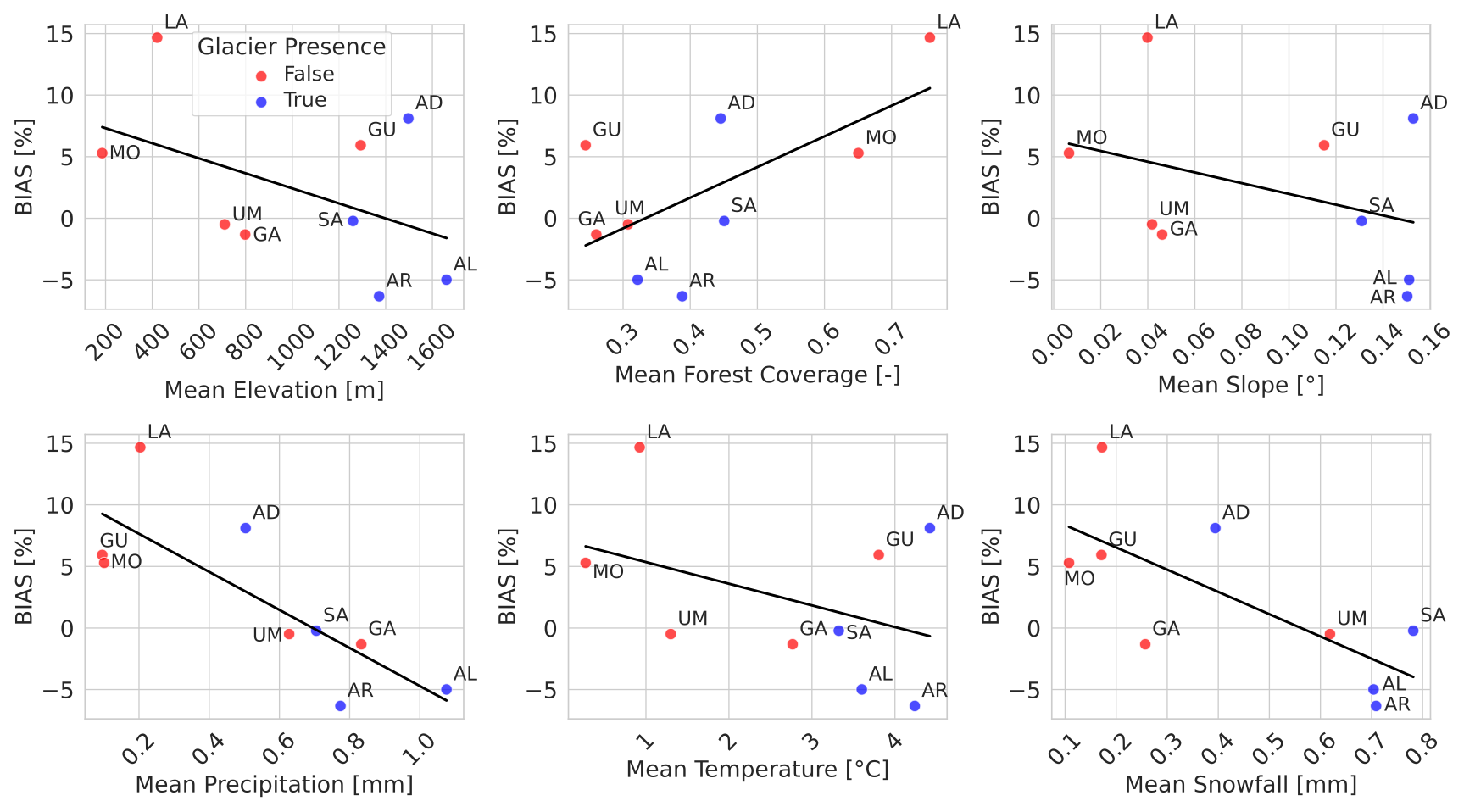
Figure 8 Bias of SCF obtained using EO-C_m in relation to selected physiographic and climatic features. Basin identifiers are indicated by their initial letters. Glacierized basins are marked in blue, and non-glacierized basins in red.

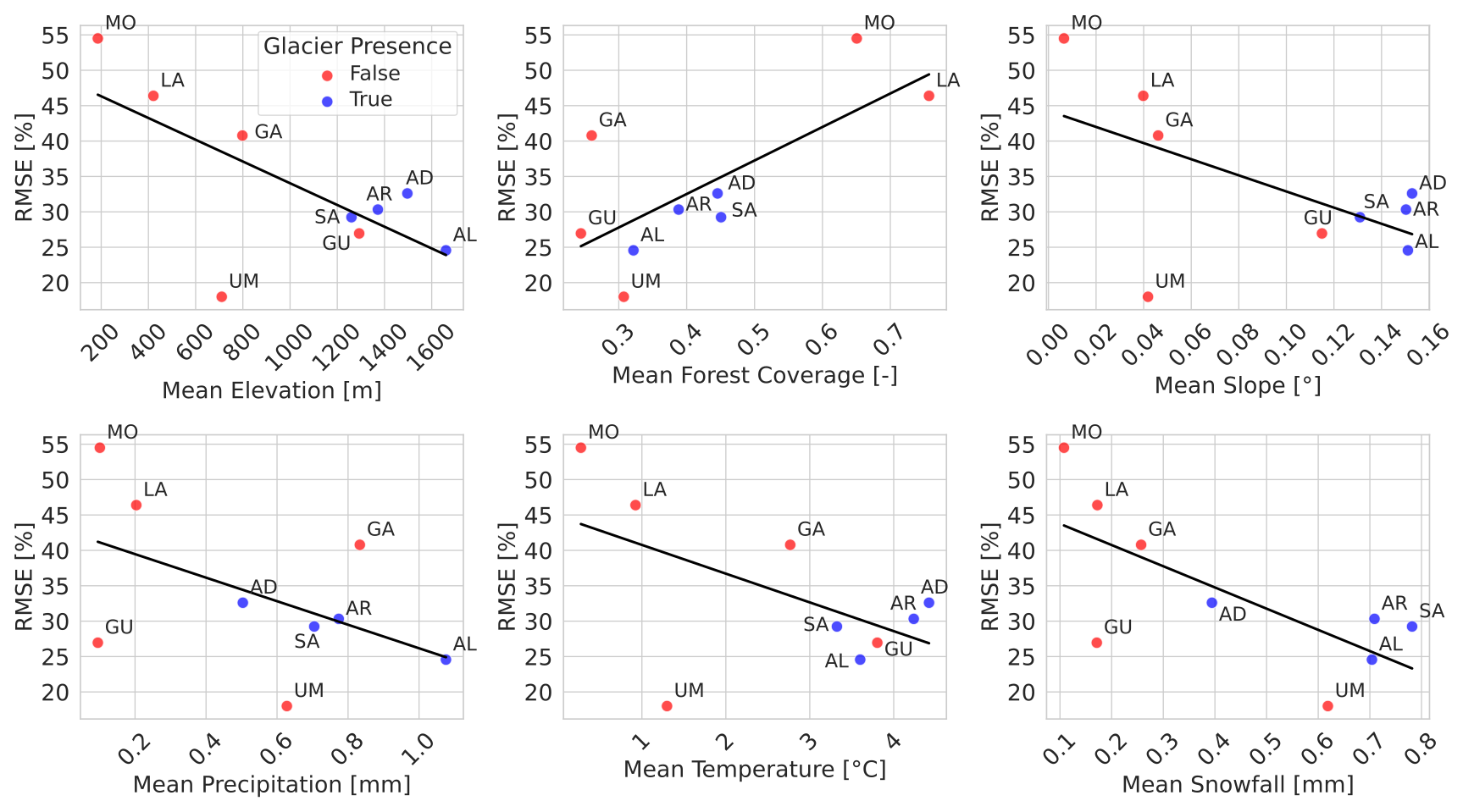
Figure 9 Root mean square error of SCF obtained using EO-C_m in relation to selected physiographic and climatic features. Basin identifiers are indicated by their initial letters. Glacierized basins are marked in blue, and non-glacierized basins in red.

The analysis shows that errors tend to be larger in lower-elevation and flatter catchments, with a similar increase associated with higher forest coverage. For the climatic features, we find an inverse relationship with RMSE: basins characterized by higher precipitation and snowfall generally exhibit lower errors. This aligns with expectations, as lower precipitation – particularly in the form of snowfall – typically results in more ephemeral snow cover, increasing the prevalence of fractional snow-covered areas, which are more prone to both detection and modeling errors. Glacierized catchments do not, on average, display substantially different performance relative to non-glacierized ones. The Umeälven basin always shows markedly lower RMSE. This is likely due to its prolonged and near-complete seasonal snow cover, which reduces snow-cover variability and associated modeling errors.

It is also interesting to analyse the monthly evolution of bias and RMSE, as shown in Fig. 10. Overall, model performance tends to deteriorate during the summer months across all basins, reflecting the snow depletion phase. This reduction in performance is partly driven by the smaller number of snow-covered pixels considered (snow-free pixels are excluded), which are often characterized by fractional snow cover and thus more prone to errors. Nevertheless, despite this seasonal decline, we generally observe an improvement when applying EO-C_m.

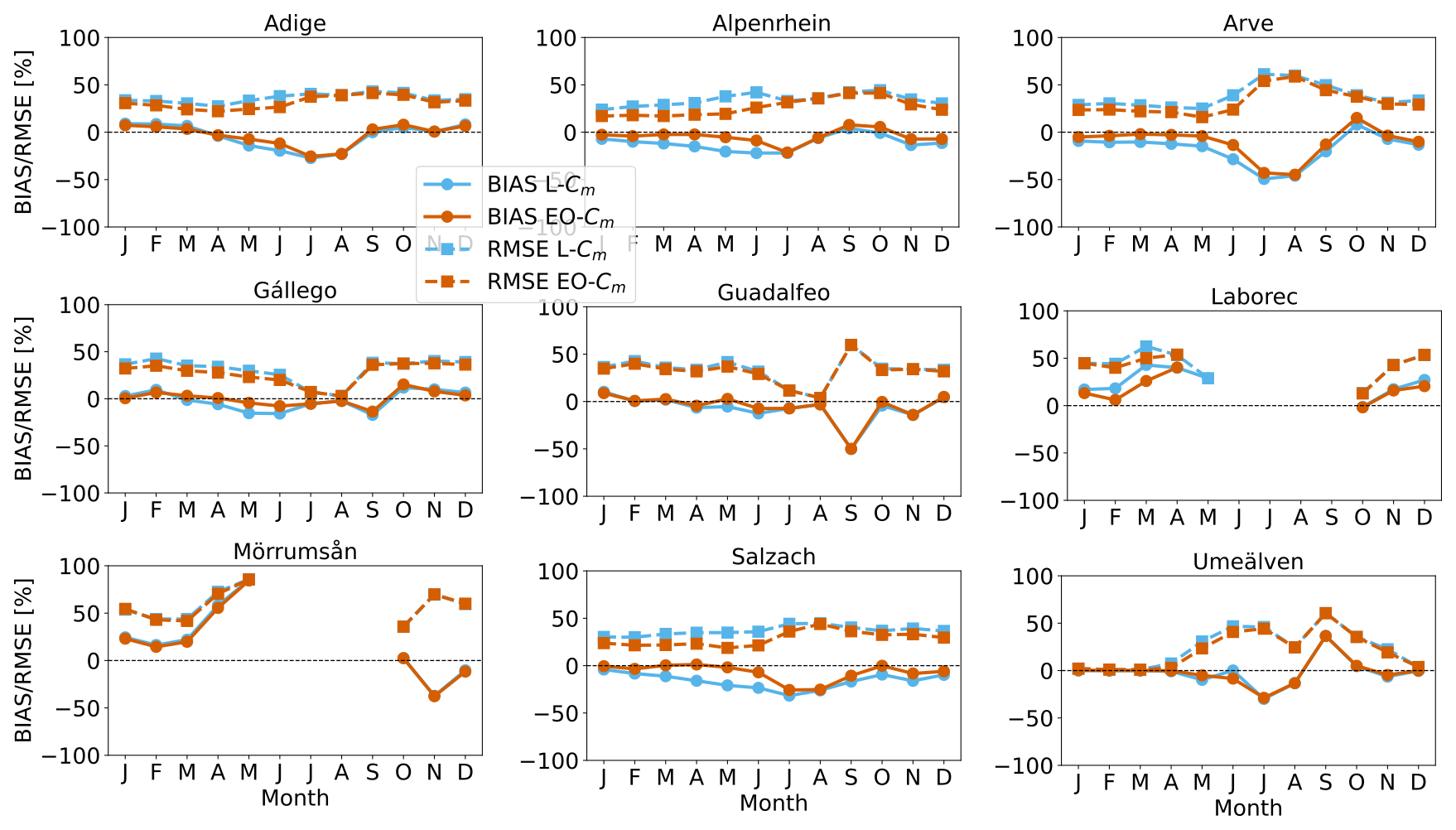
Figure 10 Monthly BIAS and RMSE trends for the nine river basins. In cyan, the BIAS (solid line marked with dots) and RMSE (dashed line marked with squares) calculated by using L-C_m. In orange, the same calculated with EO-C_m.

4.3 Snow Water Equivalent Intercomparison

To fully assess the performance of the snow module before and after snow melt coefficient recalibration, spatialized SWE maps would ideally serve as a reference. However, a comprehensive analysis is not feasible due to significant challenges in data availability and usability. Given the spatial resolution of a LISFLOOD pixel, in-situ measurements are unreliable proxies, as they fail to capture intra-pixel variability – particularly in basins with complex topography. Additionally, SWE data is often missing, and when only snow height measurements are available, converting them to SWE requires assumptions about snow density, introducing further uncertainty. Remote sensing products also have limitations. The accuracy of SWE derived from microwave sensors is affected by factors such as vegetation cover, topography, and snow type (Pulliainen et al., 2020). Furthermore, many available datasets, including those from the Copernicus Land Monitoring Service, have coarse spatial resolutions and often exclude mountain areas, further restricting their applicability (Takala et al., 2011). Therefore, we propose an intercomparison with SWE estimates from two different models in the Adige and in a subchatchment of the Alpenrhein, the Dischma Valley. For the Adige, we consider the IT-SNOW reanalysis dataset (Avanzi et al., 2024) (see Fig. 11). For Dischma, we compare our results with the Swiss Operational Snow-Hydrological (OSHD) model system, available for the first five seasons (Mott, 2023; Mott et al., 2023) (see Fig. 12). The metrics are reported in Table 5.

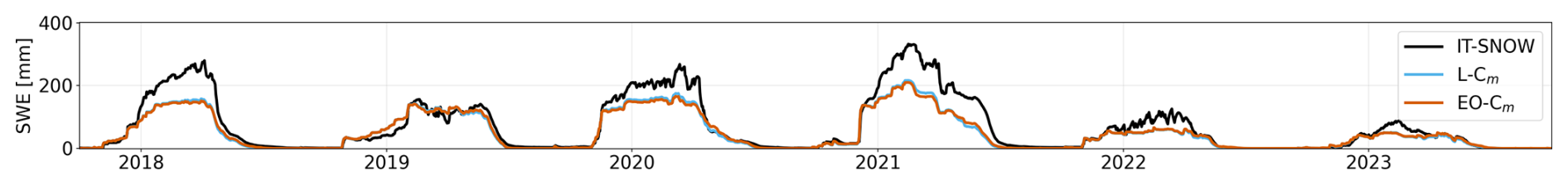
Figure 11 SWE time-series for the Adige river basin. In black the simulation from IT-SNOW, in cyan the LISFLOOD simulation using the standard EFAS5 snowmelt coefficient (L-C_m), and in orange the LISFLOOD simulation using the EO-optimized coefficient (EO-C_m).

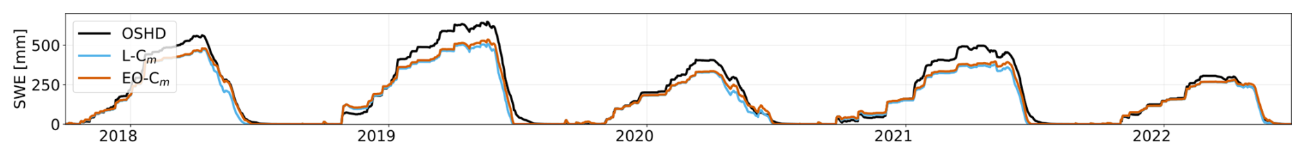
Figure 12 SWE time-series for the Dischma (Alpenrhein). In black the simulation from OSHD, in cyan the LISFLOOD simulation using the standard EFAS5 snowmelt coefficient (L-C_m), and in orange the LISFLOOD simulation using the EO-optimized coefficient (EO-C_m).

Table 5 Evaluation of LISFLOOD SWE in terms of BIAS, RMSE, and correlation using IT-SNOW as the benchmark for Adige and OSHD for Dischma (Alpenrhein). The two different snowmelt coefficients L-C_m, EO-C_m were utilized. Pixels where both the target and reference SCF are snow-free are excluded from the analysis.

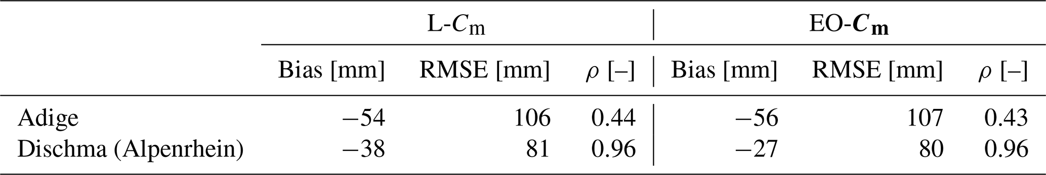
The results confirm a generally good agreement but also highlight LISFLOOD’s tendency to underestimate SWE compared to the other models in both basins. These differences are most likely linked to discrepancies in precipitation input data. Notably, IT-SNOW assimilates snow height measurements, which can enhance the accuracy of accumulation estimates. Discrepancies in the input forcings might explain the general low correlation for the Adige ($\mathrm{0.44}/\mathrm{0.43}$), while for Dischma we obtain a very high correlation (0.96) both previous and after C_m replacement. Notably, especially for the Dischma Valley the depletion curve is better captured when using EO-C_m. However, for both basins we obtain comparable or slightly improved metrics aligning with expectations based on the SCA comparison. Interestingly, we did not observe worse performance in representing different conditions, such as snow drought events, which appear to be reasonably well reproduced by both the standard and EO-C_m. This is particularly evident in the Adige basin during the 2021/22 and 2022/23 seasons. It should be noted that this analysis is not exhaustive, as it relies solely on intercomparison with other models with inherent limitations stemming from model parameterizations and the quality of forcing inputs. Therefore, the analysis lacks validation against reference data.

4.4 Effects on Long-Term LISFLOOD Simulations

In this section, we evaluate the hydrological response to post-replacement of the snowmelt coefficient (EO-C_m), with results compared against benchmark simulations using the standard L-C_m. Note that, as explained in Sect. 2.2.1, all the other parameters are kept unchanged, following EFAS5. Results are shown as daily averages calculated only for periods with available observations (Fig. 13). Reported variables include SWE, snowmelt, and discharge, all expressed in mm d⁻¹. Dashed lines in the figure denote the 10th and 90th percentiles of the time series, indicating variability in the modelled hydrological response.

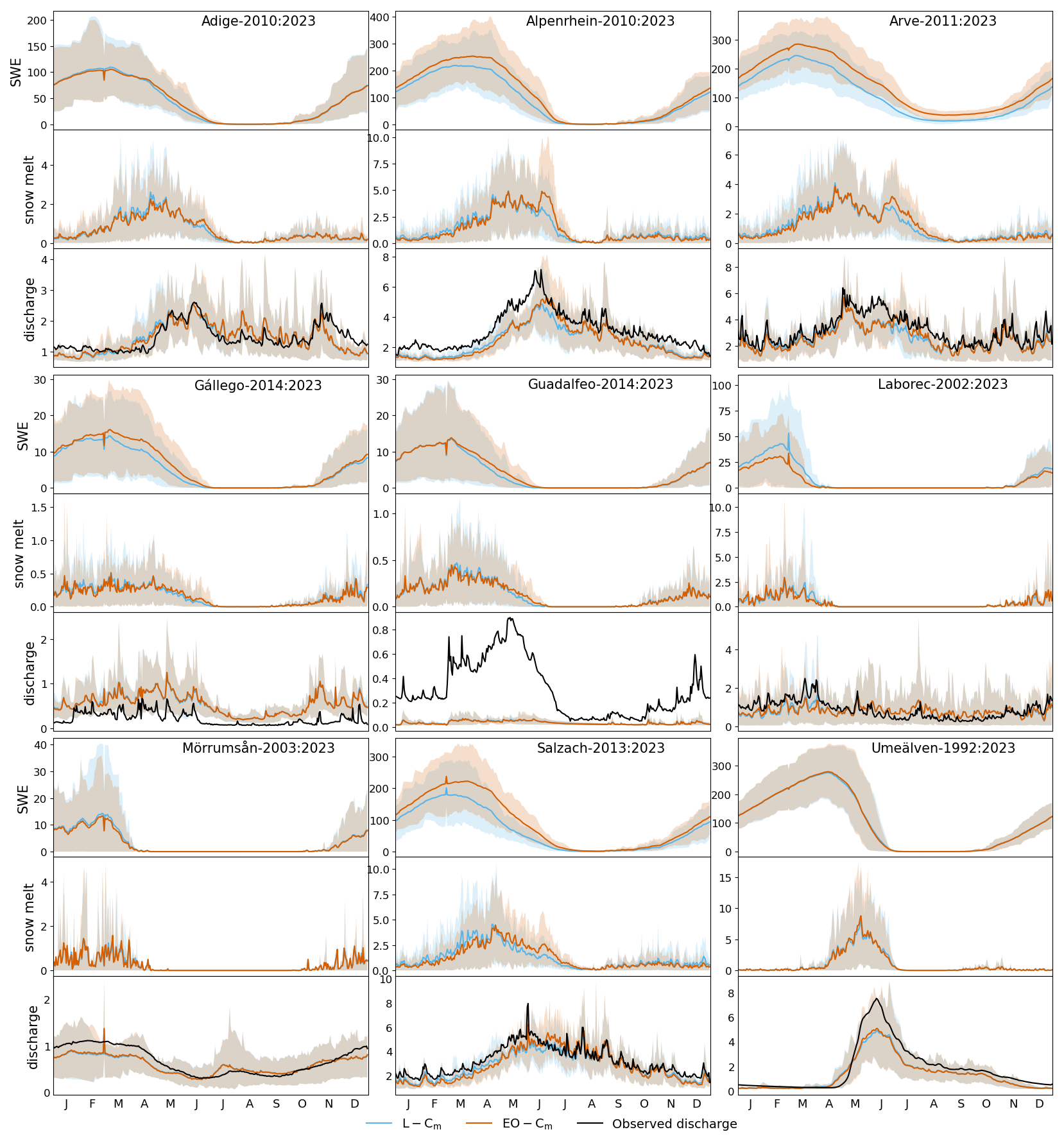
Figure 13 Daily averages of SWE, snowmelt and discharge, in mm d⁻¹. In black, the daily averages of observed river discharge, in cyan the benchmark run calculated using L-C_m, and in orange the daily averages from the run with the new calibrated coefficient EO-C_m.

In most catchments, the new EO-C_m affects the timing of both accumulation and melting phases, which in some cases also influences the timing and magnitude of runoff. In the Adige basin, the behavior of the snow cover is similar in both runs. The benchmark has a higher peak in SWE in March, but a higher depletion as well from April onward. This is reflected in the snowmelt, where the EO-run shows a slight shift in the timing of snowmelt, with lower snowmelt between March and May and higher in June, compared to EFAS5. This shift has minimal impact on the generation of discharge. Notably, the snowmelt coefficient assigned through the regionalization approach aligns closely with that derived from the EO-SCA.

In the Alpenrhein, Gállego and Salzach basins, the new EO-runs show an increase in snow accumulation, driven by reduced snowmelt before the peak. This results in a higher magnitude of snowmelt and a shift in its timing, with the peak occurring later compared to the benchmark. The effect of the newly calibrated snowmelt coefficient extends to discharge, leading to increased discharge during the snowmelt phase and reduced discharge during the snow accumulation phase. This shift does not affect the daily average discharge in the Gállego basin, but it does influence the Alpenrhein River, where it improves the agreement with observations during July and August. In case of Salzach basin the increased discharge between June and July is overestimating the observed discharge, with EFAS5 having a better match with observations.

The EO-run of the Arve basin shows a positive bias in SWE, which is only partially reflected in snowmelt since more SWE does not melt during the summer period. Snowmelt is significantly higher between June and August, and matching better observed river discharge for the same period.

In the Guadalfeo basin, a slight decrease in the snowmelt peak is observed, occurring in March, with no impact on total runoff. The model heavily underestimates river discharge compared to observations. This poor performance may be partly due to the regionalization of parameter assignment and/or the inclusion of the Rules reservoir in the model for the entire simulation period (1992–2023), despite it was opened in 2004. The observed mean daily values account for 13 years when the reservoir did not yet exist, as it was commissioned in 2004, whereas the simulation assumes the reservoir has been present throughout the entire period. In the Laborec basin, snow cover is reduced and snowmelt occurs earlier, peaking in February. Extreme values are reduced, with the 90th percentile decreasing from 60 to 52 mm for snow cover and from 100 to 80 mm per month for snowmelt. The discharge increases in January and February but decreases in March. While the flow regime is broadly similar to observations, notable differences remain with observed runoff being 30 % higher than both simulations. In the Swedish catchments Mörrumsån and Umeälven, no significant differences were found in mean daily values. The only noticeable deviation occurred in the 90th percentile of SWE in Mörrumsån, reflecting a period of high snow accumulation, followed by a sharp drop in SWE and increased snowmelt, likely driven by a temperature spike.

The performance statistic KGE, for the period with available observations, is reported in Table 6. Since the EO-C_m model was not recalibrated, a general decline in KGE and related metrics was expected. However, in most cases, the differences in metrics are not significant, and in some instances, there are improvements, which are highlighted in bold in Table 6. Across all catchments, the bias component remains virtually identical between the EO-C_m and L-C_m experiments, indicating that incorporating EO-C_m does not systematically increase or decrease the total volume of simulated discharge. A slight degradation is observed in correlation, particularly in the Laborec basin, suggesting that EO-C_m somewhat reduces the accuracy in capturing the timing of peak flows. This is particularly important in the operational context of EFAS5, where changes in correlation directly impact the system’s ability to anticipate or delay peak flows. The impact on variability is more heterogeneous: improvements are observed in the Adige, Guadalfeo, and Umeälven basins, while reductions occur in the Salzach and Alpenrhein. This pattern implies that EO-C_m can have a positive effect on representing interannual flow fluctuations in some basins, but not universally. Overall, model performance increases in the Adige and Mörrumsån basins following the introduction of EO-C_m, whereas noticeable declines occur in the Alpenrhein, Laborec, and Salzach.

Table 6 Hydrological performance of current LISFLOOD configuration (EFAS5) and LISFLOOD run with the new snowmelt coefficient. Together with the KGE, the bias ratio (β), the Pearson correlation (r) and the variability ratio (γ) are reported. In bold values with metrics that perform better using the EO-C_m snowmelt coefficient compared to EFAS5.

Figure 14 presents monthly Kling-Gupta Efficiency (KGE) values for both EO-C_m (cyan) and L-C_m (orange) LISFLOOD runs. In most basins, such as Adige, Alpenrhein, Arve, Mörrumsån, and Salzach, both experiments achieve consistently high KGE scores (generally above 0.5), indicating robust model performance throughout the year. Conversely, in basins such as Gállego, Guadalfeo, and Umeälven, the simulations exhibit lower and more variable KGE scores, with several months showing negative values; this suggests poor performance and notable mismatches between simulated and observed river flows. The Gállego and the Guadalfeo basins in particular exhibit poor KGE in most months, which is reflected in their negative KGE in Table 6; the EO-C_m did not yield significant improvements/worsening in these catchments. Performance differences between the two experiments are most pronounced in specific seasons. The EO-C_m model run outperforms the L-C_m run in the melting season of Arve and Alpenhrein, as well as in the snow accumulation season of the Adige and Mörrumsån basins. A decreased performance is observed for most months in the Salzach basin, while Laborec shows mixed results, with slight improvement in December and January and a decline in March and April. As stated in Sect. 2.2.1, the comparison is between a calibrated LISFLOOD run (L-C_m) and an uncalibrated one (EO-C_m). A deterioration in the performance of the EO-C_m simulation is therefore expected, since the remaining 13 parameters were not subject to calibration. Conversely, any improvement in KGE, its three components, or daily average performance would indicate that a calibrated EO-C_m configuration of LISFLOOD could potentially yield superior results. Moreover, because the current calibration strategy relies on a single parameter to represent snow processes, it is likely that the calibration compensates for structural or process-level deficiencies by adjusting other parameters, potentially masking the true contribution of the snow-related parameter.

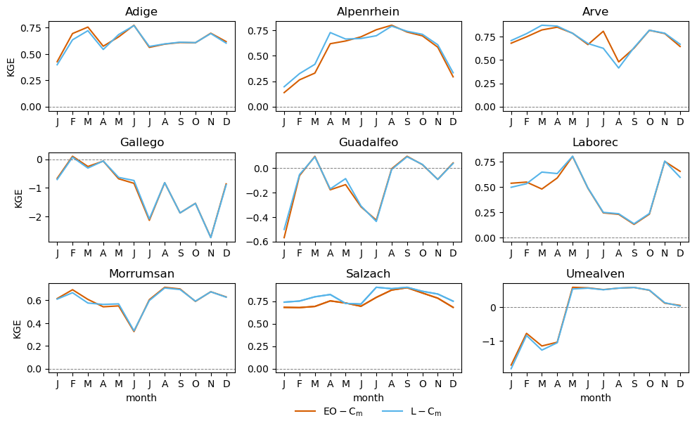
Figure 14 Monthly KGE calculated for both LISFLOOD runs against observed discharge. In cyan the benchmark run calculated using L-C_m, and in orange the run with the new calibrated coefficient EO-C_m.

Figure 15 presents the NED for each catchment. Darker colors indicate river sections where the two models produce similar daily discharge (low NED), while lighter colors highlight areas of stronger divergence.

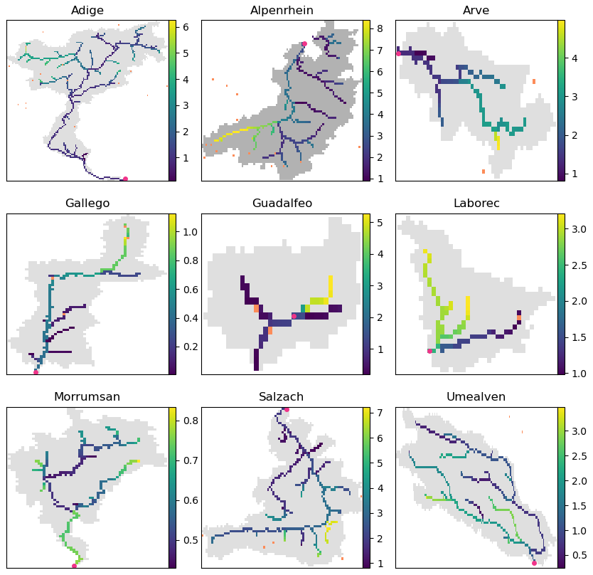
Figure 15 Normalized Euclidean Distance between daily discharge of LISFLOOD model as per in EFAS5 and the LISFLOOD model run with the EO-C_m coefficient. Light colors mean that the discharge are different, dark colors mean that discharges are similar. Reservoirs are highlighted in orange in the figure.

The spatially heterogeneous EO-C_m shows a marked local impact in some river reaches with small upstream areas, where differences between model outputs are more evident. This influence decreases progressively downstream as localized effects are smoothed along the flow path. By the time discharge reaches the calibration points, typically located further downstream, the impact becomes negligible, as the calibration process compensates for or overrides local parameter variations. The Gállego and Mörrumsån basins exhibit the least effect from the EO-C_m implementation, with maximum NED values reaching only 1. Laborec and Umeälven follow, displaying peak NED values up to 3. In the remaining basins, most river reaches have NED values below 4, although some specific sections show higher localized NED values.

Reservoirs generally have minimal effect on the differences between the two simulated discharges across most basins. However, in the Gállego and Adige basins, distinct impacts are observed at the outflow of a single reservoir in each basin: in Adige, this occurs at the first upstream reservoir in the north-west area; in the Gállego, at the second reservoir moving downstream from the headwaters. In both cases, the grid cell immediately downstream of the reservoir shows greater differences than the grid cell directly upstream.

5 Discussion

This study tested the snow module of LISFLOOD and evaluated the outcomes of a post-replacement of the snowmelt coefficient with EO-calibrated values after a standard streamflow calibration. The approach improves the representation of snow cover without deteriorating hydrological performance and without requiring a full, time-consuming model recalibration. Here, we discuss outcomes and limitations of this study.

In its current EFAS5 setup, LISFLOOD already provides reasonable basin-scale estimates of SCA and SWE. However, optimizing the snowmelt coefficient with EO data improves the representation of SCF during the depletion phase, as C_m optimization reduces discrepancies between modelled and observed SCF. This enhances the consistency of the melting phase with satellite-observed depletion trends (Fig. 6), particularly in basins such as the Alpenrhein, Arve, and Salzach, where a single, well-defined accumulation–melt cycle facilitates alignment. In contrast, basins with ephemeral snow cover, such as the Laborec and Mörrumsån, show poorer performance. Additional uncertainties also stem from limitations in the EO product itself: persistent cloud cover can lead to errors in SCF reconstruction, while forested areas remain problematic for optical sensors that cannot detect snow beneath the canopy.

We acknowledge also limitations linked to the LISFLOOD model. First, it operates at a coarse spatial resolution, which may not adequately capture processes in regions with complex topography. This choice is inherent to its role as a continental, operational model. Furthermore, the snow module is relatively simple and does not include glaciers. In this work, the accumulation scheme was not recalibrated, and key parameters, e.g., the temperature threshold for rain–snow partitioning, were not adjusted, even though they strongly influence snowpack evolution. As a result, errors introduced during the accumulation phase remain uncompensated in the calibration. Uncertainties in the forcing inputs, particularly biases in precipitation, are likely a dominant source of error, affecting snow accumulation regardless of model parameterization. The temporal stability of the EO-C_m (Fig. 5) likely reflects systematic elevation dependent biases in the precipitation forcing. In particular, poorly represented orographic gradients and snow undercatch – arising from coarse model resolution and the absence of dedicated parameters – likely explain the spatial variability in EO-C_m, which compensates for these errors. Improving precipitation datasets and explicitly calibrating accumulation-related parameters would likely enhance snow process representation in LISFLOOD. However, we emphasize that SCF data alone may be insufficient to fully constrain the snow accumulation process, as precipitation events over existing snow cover do not alter SCF and therefore provide no information about snow depth or volume. In general, snow cover represents non-volumetric information and thus offers only partial constraints on snow processes (Pellicciotti et al., 2012). We also acknowledge – as mentioned in Appendix B – challenges in tuning of the parameter k_accum, which is suggested to be performed during the first snow event. These limitations mainly arise from potential temporal mismatches between modelled SWE and EO observations, as well as from the inclusion of ephemeral early-season snow events that may not be fully representative of the seasonal snowpack.

Furthermore, assuming a constant snowmelt coefficient over time may be a strong assumption. Although our analysis in Sect. 4.1 showed an overall stability of the EO-C_m distribution across different seasons – and demonstrated that both EFAS5 and the new coefficient were capable of reproducing a range of conditions, from wetter seasons to snow-drought periods – variations in snow density, shallow snowpacks, or the presence of wind crusts, among others, can significantly affect snowmelt dynamics. While seasonality is accounted for through the addition of C_seas, this might not fully capture variations in snowpack characteristics. The sinusoidal function that defines C_seas merely adds a value in the range of ±0.5 mm (°C d)⁻¹, without considering key geographical and topographical factors such as latitude, altitude, or shading, slope and aspect, which influence snowmelt. These limitations are intrinsic to temperature-index models and may be mitigated through enhanced temperature-index formulations or energy-balance models (Ruelland, 2023). Given the above considerations and in light of our analysis, future work on the LISFLOOD snow module should focus on improving the snowfall/rainfall partitioning, accumulation phase, variation of snowmelt coefficient and glacier dynamics.

Our findings highlight notable differences in both the spatial distribution and the magnitude of C_m across the two calibration approaches. Despite these substantial variations, the EO-based coefficient primarily influences the timing of snow accumulation and melt phases. In some river basins, this altered timing propagates into seasonal differences in the timing and magnitude of river discharge, mainly during and immediately following the snowmelt period; however, differences in KGE and daily average discharge remain minimal in the catchments analyzed. These results are consistent with previous studies, which reported relatively modest improvements in streamflow but greater gains in producing more realistic snow cover patterns (He et al., 2014). Model results show that EFAS5 and current calibration routine generally provides a good estimation on snowmelt dynamics, on average at catchment level. However, this conclusion was not obvious given the large number of calibrated parameters in LISFLOOD (14 in total) and the possibility for EFAS5 to have a parameter set that could reproduce well river discharge but not snow dynamics. A large number of parameters in distributed hydrological models can indeed result in a set of calibrated parameters that do not represent some key processes well, such as snow processes in this exercise, and instead exhibit compensation effects with other parameters in order to maximize the objective function (KGE) and the representation of a single process (river discharge) (Beven, 2006; Finger et al., 2015).

Since calibration maximizes KGE, we do not expect lower values if the model were completely recalibrated with the EO-derived coefficient. This suggests that a two-step calibration, first constraining the snow melt coefficient with EO data followed by recalibration of the remaining parameters, could achieve similar or even improved performance in terms of KGE with the advantage of reducing equifinality. Such an approach would allow for a more realistic representation of snow processes in LISFLOOD without compromising consistency at the larger scale, which is particularly valuable for applications in snow-dominated basins. However, given the importance of LISFLOOD at global and European level, a two-step approach would have to go through an increased number of tests. Previous studies of sequential calibration have often reported degradation in streamflow performance compared to our results, though differences in model structure, catchment size, and calibration strategies complicate direct comparison. For example, (Xiao et al., 2022) and (Franz and Karsten, 2013) did not perform pixel-wise calibration of snow-related parameters but instead aggregated them by hydrological response units (HRUs) or snow bands. Catchment areas in those studies were also typically an order of magnitude smaller than those considered here. Our NED analysis indicates that shifts in SWE and snowmelt in Alpine basins warrant caution when interpreting simulated discharge upstream of calibration stations, particularly in smaller sub-catchments.

Ruelland (2024) found slight degradation in streamflow performance under sequential calibration for European catchments ranging from 45 to 3580 km² and recommended a multi-objective approach incorporating SWE point observations. While this is one of the most comprehensive studies evaluating the inclusion of SCF and SWE in calibration, direct comparison remains difficult due to differences in model structure, performance metrics, and snow calibration strategies. Moreover, incorporating SWE in-situ observations at continental or global scale is challenging. Even the EO-SCF dataset used here, which combines HR and LR products, improved spatial detail but increased data management complexity. For large-scale operational applications, simpler, ready-to-use datasets may be more practical (Appendix A). Another promising direction would be to derive spatially distributed snowmelt coefficients from meteorological, geographic, and land-cover predictors, or to explore data-driven approaches that estimate snow accumulation and melt using machine learning techniques (Umirbekov et al., 2024).

Future work should place greater emphasis on improving the representation of the accumulation phase and refining model structure, and should evaluate these enhancements in smaller headwater catchments, especially in light of the divergence revealed by our NED analysis. Such divergence is particularly consequential for water management applications in snow-dominated regions, as it directly affects inflow variability that governs reservoir storage, operational strategies, and the timing and volume of water available for hydropower generation, irrigation, and flood control. At the same time, a more accurate representation of snow processes in headwater basins could improve operational flood forecasting within EFAS, where warnings are issued at the river-pixel scale. If EO-based calibration enhances the simulation of streamflow regimes in small, snow-driven catchments, it may increase the reliability of flood warnings in these areas, which is especially relevant given the decline in EFAS forecast performance with decreasing catchment area (Casado-Rodríguez et al., 2025).

In conclusion, our results highlight the potential of EO data for constraining the snowmelt coefficient, but also emphasize the need for further research given the mentioned limitations. In addition to SCF, more complementary observations such as in-situ SWE observations should be incorporated, and sensitivity analyses of the SCF–SWE transformation should be undertaken. In mountainous regions, discharge data from smaller upstream catchments could provide valuable benchmarks to better evaluate and refine model performance.

6 Conclusions

In this work, we assessed the performance and limitations of the LISFLOOD snow module in simulating snowmelt and snow water balances across diverse European watersheds. By re-calibrating the snowmelt coefficient (C_m) using highly detailed EO-derived daily snow cover data from high-resolution optical sensors, we evaluated: (i) how well current EFAS5 setup reproduces snow and streamflow; (ii) whether EO-derived C_m improves snow process realism; and (iii) the impact of such adjustments on hydrological performance across diverse European catchments.

To this purpose, we derived EO snow cover from multi-source optical sensors. The daily gap-filled SCA, obtained from MODIS and Sentinel-2 data, was used to calibrate a spatially distributed snowmelt coefficient. We implemented and evaluated an appropriate snow cover parameterization for converting SWE into SCF to effectively evaluate snow depletion. The snowmelt coefficient was derived through an optimization-based approach that minimizes the error between simulated and observed SCF.

The primary objective of comparing the EFAS5 setup with the same setup incorporating the independently calibrated snowmelt coefficient was to evaluate whether recalibrating this single parameter would significantly impact the hydrological cycle. Additionally, this approach enabled us to assess the robustness of the full LISFLOOD calibration – which involves 14 parameters – in accurately reproducing snow dynamics.

Our main findings indicate that the current LISFLOOD snow module, calibrated using a standard hydrological approach, already produces satisfactory results at basin scale. When evaluated against EO-SCF, the model’s bias ranged from −1 % (Gállego) to 22 % (Laborec), with RMSE values between 20 % (Umeälven) and 55 % (Mörrumsån). These results highlight, however, that fractional snow cover is often misrepresented in the current setup. A dedicated calibration of the degree-day factor improved performance, particularly during melting periods, with gains of up to 8 % in both bias and RMSE. Despite these improvements in snow metrics, discharge simulations remained largely unchanged, reflecting the quasi-equifinal role of the snowmelt coefficient on streamflow. The main differences appeared in the timing and magnitude of snow accumulation and melting, which in turn influenced the timing of runoff contributions. This shows that discharge-based calibration alone compensates for snow misrepresentations, often “getting the right result for the wrong reasons” (Kirchner, 2006).

In conclusion, our findings suggest that a sequential calibration approach – first adjusting the snowmelt coefficient using EO-derived SCA, followed by a post calibration of streamflow – can be the correct approach to pursue. Furthermore, we find that a standard calibration on streamflow alone, followed by a post-replacement of the snowmelt coefficient based on SCA, can still yield acceptable results without the need to recalibrate the entire model.

Although our experiments focused on LISFLOOD, both the rationale and the calibration strategies are applicable to other distributed hydrological models facing similar challenges in snow-dominated catchments.

Appendix A: Earth Observation Snow Cover Dataset

In the methodological Sect. 2.1, we saw that the approach presented by Premier et al. (2021) to creating a continuous, gap-filled daily SCA dataset relies on multi-resolution optical data, in detail low-resolution (LR) SCF and high-resolution (HR) snow maps. A widely used operational LR SCF product with a long record (more than 20 years) is the MOD10A1 product derived from MODIS. Similarly, to obtain HR snow cover maps from Sentinel-2, we can utilize existing operational products such as the Copernicus Fractional Snow Cover (FSC) product. However, the use of other alternative datasets is also possible. Among others, we investigated the datasets listed in Table A1.

SnowFLAKES is also derived from Sentinel-2 and represents an alternative to FSC. It employs a more advanced algorithm, specifically the Snow extent from applying a Flexible Learning Algorithm using KErnel-based Spectral unmixing developed internally at Eurac (Barella et al., 2022). The method is based on an unsupervised machine learning algorithm. While we have observed an improvement in snow detection, particularly in challenging situations such as shadowed pixels, the algorithm is still experimental, and the maps are not yet available for operational use. Similarly, an alternative to MOD10A1 but with shorter temporal coverage (from 2012 onward) is represented by VNP10A1, while ESC-H provides an alternative with coarser spatial resolution. There are also operational products, such as GFSC and VNP10A1F, which provide gap-filled time-series to address cloud obstruction.

Gascoin et al. (2019); Copernicus Land Monitoring Service (2021)Barella et al. (2022)Hall and Riggs (2021)Riggs and Hall (2023)H-SAF Team (2020)Copernicus Land Monitoring Service (2021)Riggs and Hall (2022)

Table A1 Overview of snow cover products, their sources, native and resampled spatial resolutions, and temporal resolutions.

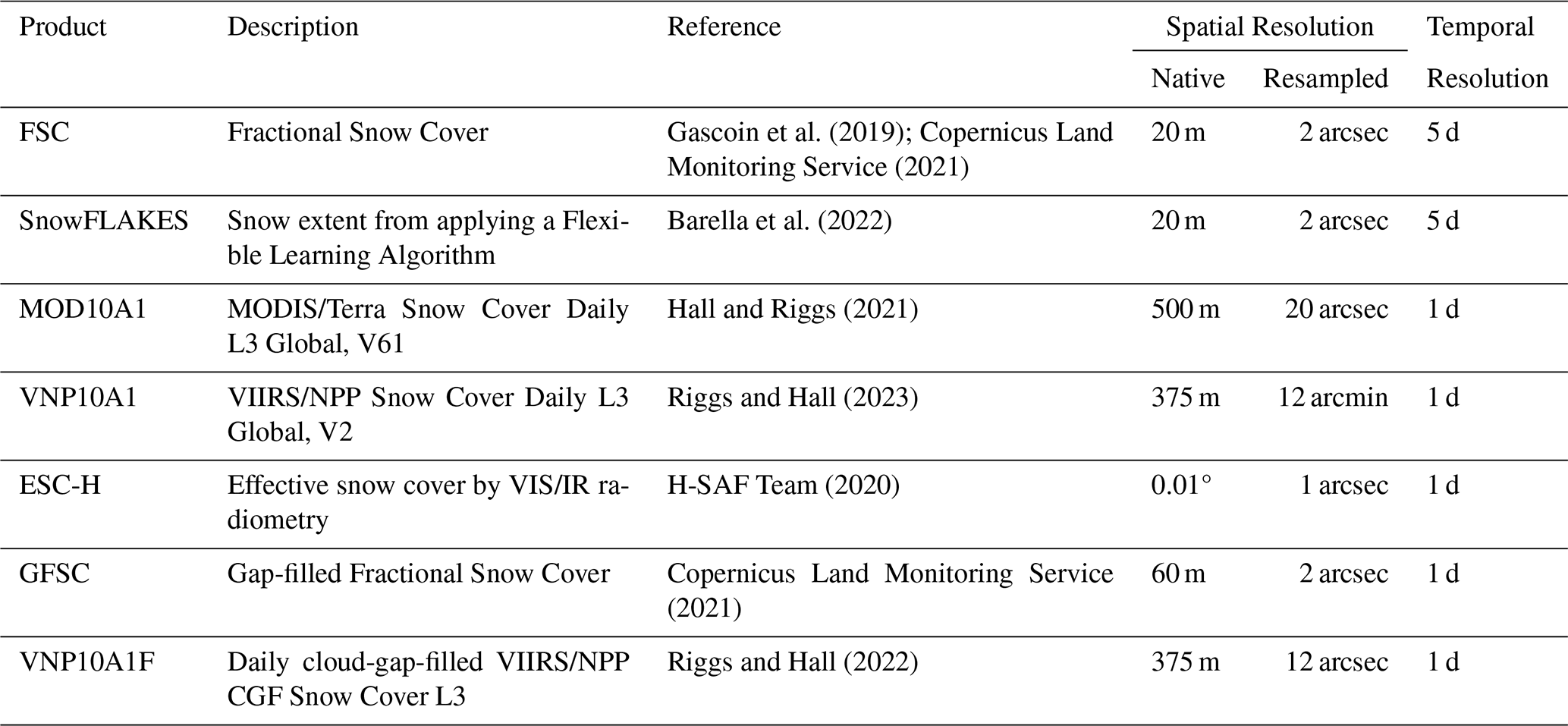
While many possible combinations are possible, we propose obtaining a daily gap-filled SCA by merging FSC and MOD10A1, referred here as Copernicus-derived gap-filled SCA (C-GSCA). This ensures both operational use and the possibility to generate data back in time. However, for some selected basins, we tested the combination of MOD10A1 with SnowFLAKES, referred to here as SnowFLAKES-derived gap-filled SCA (S-GSCA).

Considering C-GSCA as the benchmark, we conducted an intercomparison to assess the usability of different products, focusing on gaps primarily caused by cloud cover or satellite design. This analysis evaluates the potential of the analyzed datasets for use either as standalone inputs or within a merging approach by providing an overview of their agreement. Prior to the analysis, all products were resampled and aligned to a common grid to ensure comparability. Specifically, each product was resampled to a resolution close to that of the original data and structured as an exact submultiple of the LISFLOOD grid, as shown in Table A1.

In Fig. A1, we provide an overview of the available data for the different basins, including the average percentage of cloud-covered pixels and the total number of available images for each season. Images that are completely obstructed by clouds over the study area are excluded from these metrics. Note that, for limiting the amount of downloaded data, not all the products were tested for all the basins or seasons. This does not change the outcomes of the analysis.

To assess the agreement or disagreement among the various datasets, we computed basic metrics such as bias, RMSE, and Pearson correlation coefficient (ρ) between pairs of datasets, using C-GSCA as the reference product. The results​​​​​​​​ ​​​​​​​​ are reported in Fig. A2. For each matching date, metrics are calculated for SCF pixels aggregated to the final resolution of LISFLOOD. When the percentage of “no data” pixels exceeds approximately 10 % within a LISFLOOD cell, SCF is marked as no data (equivalent to 90 pixels for FSC, GFSC, and SnowFLAKES; 3 pixels for VNP10A1 and VNP10A1F; and 1 pixel for MOD10A1). The figure shows the average metrics for the entire available period.

The results show that LR products (MOD10A1 and VNP10A1) offer similar image counts and metrics (on average, MOD10A1: bias 1 %, RMSE 9 %, and ρ 0.73, VNP10A1: bias 0 %, RMSE 15 %, and ρ 0.63). Note that MOD10A1 is used as input in the fusion algorithm to generate C-GSCA, but its values may be adjusted based on HR data. This results in a low bias but in the presence of outliers when compared to the benchmark (see Fig. A2). Given the similar results, VNP10A1 can be considered as a valid alternative to MOD10A1. ESC-H also exhibits comparable cloud obstruction, but shows the poorest agreement (worst metrics with bias −6 %, RMSE 20 %, and ρ 0.47). The results suggest that its coarser spatial resolution reduces its utility as alternative product. In general, all datasets might not be used without a proper gap-filling algorithm.

The use of HR products (such as FSC and SnowFLAKES) is significantly constrained by their low revisit frequency, which leads to limited image availability over the year. Both products show similar levels of cloud coverage and image counts. Note that SnowFLAKES has fewer images due to the application of stricter criteria in cloud masking. The lowest availability of valid pixels for FSC is observed in the Umeälven basin, with only about 6 % of pixels available throughout the year. In addition to cloud obstruction, this basin is also affected by polar night, leading to missing acquisitions from November through February. However, this limitation does not impact the algorithm’s performance, as the basin remains fully snow-covered during this period, and acquisitions resume in time for the snowmelt season. Alpenrhein and Salzach follow, with approximately 8 % of pixels available. In contrast, the basin with the highest availability of valid pixels is Gállego with a percentage of about 19 %. Since C-GSCA is derived from FSC, we expect a good agreement (bias 0 %, RMSE 0 % and ρ 0.99). Similar performance is also observed for SnowFLAKES (bias 1 %, RMSE 7 % and ρ 0.87) and S-GSCA (bias 3 %, RMSE 9 % and ρ 0.90), with differences due to the application of a different algorithm for the snow classification. In detail, the Adige basin exhibits a slightly higher bias. A detailed visual inspection revealed that, as also stated before, FSC tends to miss snow detection in shadowed areas. This is especially highlighted for basins with complex topography.

Regarding the gap-filled products, GFSC does not offer a valid alternative; although it provides a greater number of scenes, it still suffers from substantial “no data” gaps. The lowest availability is observed for Alpenrhein, with only around 25 % of valid pixels. In fact, the gap-filling process primarily relies on propagating information from Sentinel-2 and Sentinel-1 data by using a defined temporal window (HR-S&I consortium, 2020). This is also the reason of similar performances w.r.t. the raw FSC (bias 1 %, RMSE 10 %, and ρ 0.72).

In contrast, the nearly complete gap-filled data in the VNP10A1F product represents an attractive option with potential applications. A tendency toward underestimation relative to the reference is shown but the metrics remain reliable (bias −4 %, RMSE 17 %, and ρ 0.78).

To conclude, we can state that C-GSCA is a product that by relying on HR data is expected to be more accurate w.r.t. LR data. Based on our findings, we decided to proceed with S-GSCA for the Adige basin while retaining C-GSCA for the remaining basins. In the main text, we generally refer to the time series as EO-SCA.

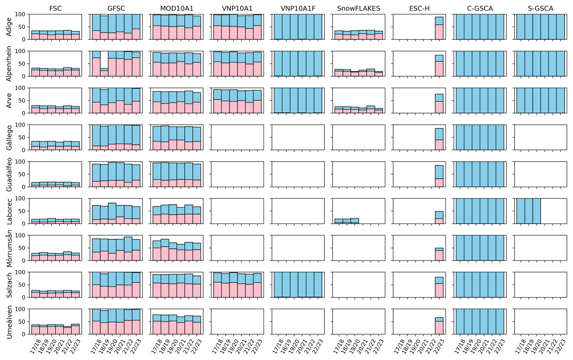
Figure A1 Overview of the available data for each basin and hydrological year. The percentage of available images throughout the year is shown in sky blue, while the percentage of cloud-covered pixels is represented in pink. Fully cloud-obstructed images are excluded from the calculations. Note that not all products were considered for every basin and season.

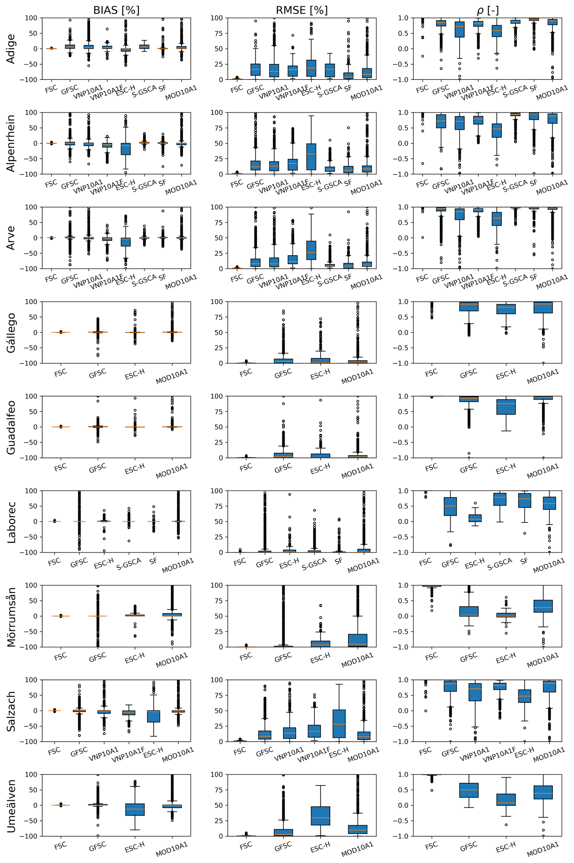
Figure A2 Boxplots of the resulting metrics (bias, RMSE and correlation) for each basin and product, using C-GSCA as the reference.

Appendix B: Snow Cover Parametrization

In this Appendix, we provide additional details and analysis regarding the snow cover parametrization described in Sect. 2.4 to convert SWE into SCF.

B1 Alternative Parametrization Approach

Here, we present results obtained using the parametrization proposed by Swenson and Lawrence (2012) (see Sect. 2.3) and compare them with the approach introduced by Zaitchik and Rodell (2009). The following relationship is used:

$$\begin{array}{}\text{(B1)}& \begin{array}{rl}\mathrm{SCF}& =min\mathit{\{}\mathrm{1}-[\exp (-\mathit{\tau }{\displaystyle \frac{\mathrm{SWE}}{{\mathrm{SWE}}_{\text{max}}}})\\ & -{\displaystyle \frac{\mathrm{SWE}}{{\mathrm{SWE}}_{\text{max}}}}\exp (-\mathit{\tau })],\mathrm{1}\mathit{\}}\end{array}\end{array}$$

where τ is the snow distribution shape parameter that relates the total amount of SWE to the SCF within the pixel. We set the snow distribution shape parameter τ to 4 globally, while SWE_max varies from 13 mm for bare soil to 40 mm for forests as suggested by Zaitchik and Rodell (2009).

By taking the EO SCF as a benchmark, we evaluated the mean bias, RMSE, and correlation for each basin by comparing the EO-SCF with the SCF generated by LISFLOOD considering the standard coefficient L-C_m under the two parametrization methods. The metrics are calculated pixel-wise and an average over time and space is computed. The results, detailed in Table B1, show improved metrics when adopting the parametrization proposed by Swenson and Lawrence (2012) for Adige, Guadalfeo and Umeälven while an improvement especially in terms of bias with the formula of Zaitchik and Rodell (2009) is shown for Alpenrhein, Arve, Laborec and Salzach while the other metrics do not show important differences. Given that the results show comparable performances and the fact that the parametrization by Swenson and Lawrence (2012) is more sophisticated, we decided to keep this approach. Therefore, all analyses and results in the main text are based on this parametrization.

Table B1 Evaluation of LISFLOOD SCF in terms of BIAS, RMSE, and correlation using the EO-SCF as the benchmark. The standard L-C_m was utilized, with SWE converted to SCF using the parametrizations proposed by Swenson and Lawrence (2012) and Zaitchik and Rodell (2009).

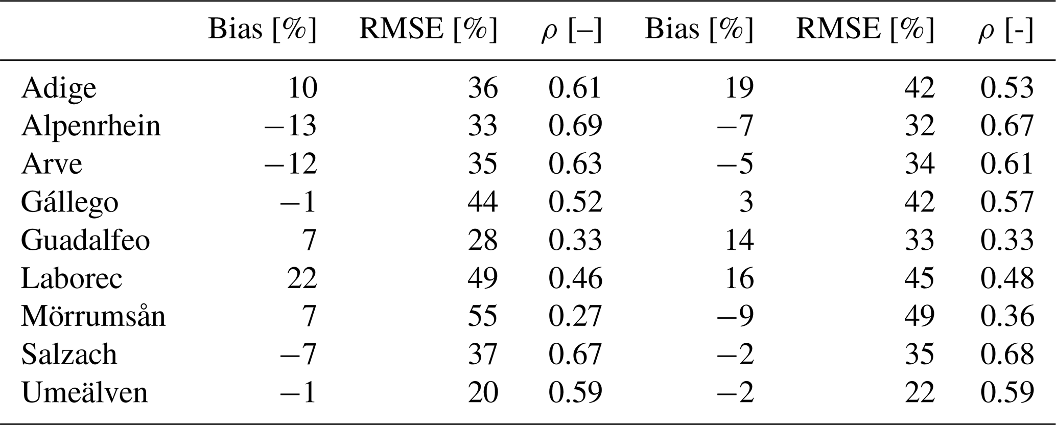
B2 Calibration of the Parameter k_accum

Here, we present the results of the calibration of the scaling parameter k_accum, as described in Sect. 2.3. The outcomes are shown in Fig. B1. As explained in Sect. 2.3, this parameter is estimated during precipitation events occurring over initially snow-free areas. We define the first day of snow accumulation as the first day on which both EO-SCF observations and LISFLOOD SWE are greater than zero, regardless of the time of year or prevailing snowpack conditions. We acknowledge that this definition may not always be optimal, particularly in cases where LISFLOOD SWE responds earlier or later than EO-SCF or when early-season snowfall may not be representative of the winter snowpack. However, averaging k_accum over five seasons helps to smooth the impact of timing mismatches and short-lived early snow events. Furthermore, when examining basin-averaged values of k_accum as shown in Fig. B1, we find that the estimated values are broadly consistent with those reported by Swenson and Lawrence (2012). We also observe systematically higher k_accum values in flatter basins, such as Mörrumsån and Umeälven, which are characterized by less complex topography. In these areas, higher k_accum values correspond to higher SCF for a given SWE, consistent with the representation of flatter pixels.

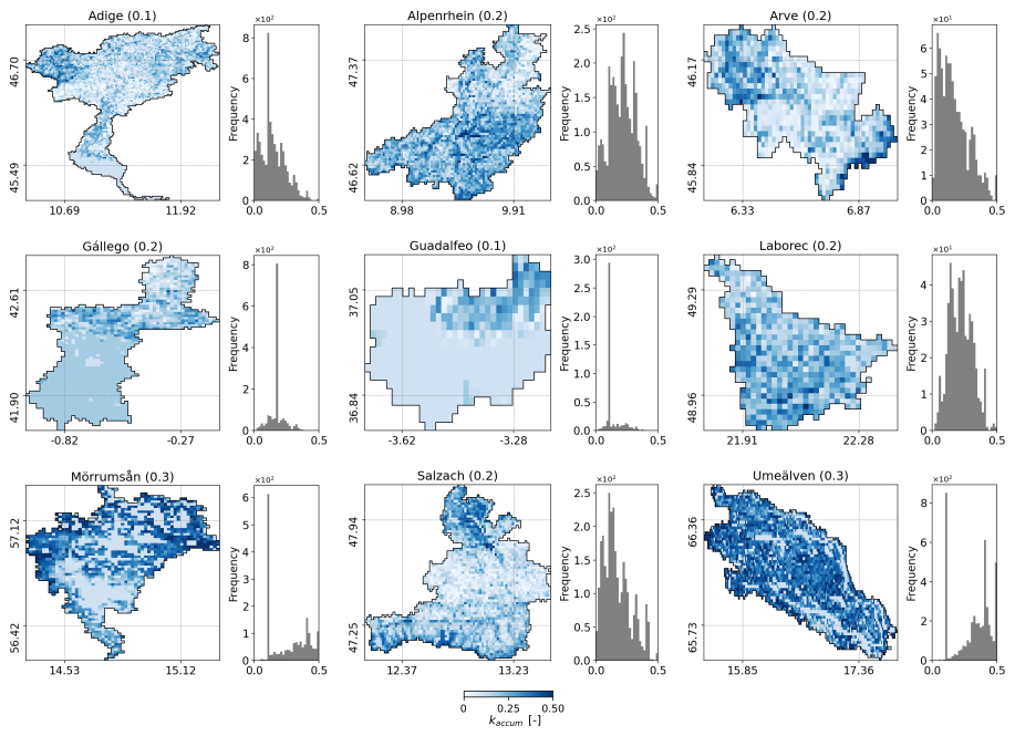
Figure B1 Scaling parameter k_accum for the nine selected basins. The corresponding histograms are also included. Average values are reported within brackets.