Uncertainties in long-term ensemble estimates of contextual evapotranspiration over southern France

Estimating evapotranspiration (ET) beyond the local or point scale is critical for water resources and ecosystem studies. Remote sensing offers a unique advantage by enabling ET monitoring at larger spatial scales than in-situ instruments. By leveraging relationships between surface biophysical parameters and terrestrial thermal emission, continuous ET can be retrieved across diverse landscapes. Herein, we apply the EVapotranspiration Assessment from SPAce (EVASPA) contextual tool over southern France, using MODIS-derived land surface temperature/emissivity (LST/E), NDVI and albedo products. The dataset spans 2004–2024, yielding 972 instantaneous ET estimates. The EVASPA ensemble integrates multiple member outputs generated from: (1) alternative formulations of evaporative fraction (EF) and ground heat flux (G), and (2) different LST and radiation inputs. Evaluation against flux tower data shows that even a simple ensemble average provides reasonable agreement, though individual member performance varies substantially. Uncertainty analyses were also performed where we looked at how each of the distinct variables (i.e., LST, radiation, EF algorithms, and G flux methods) influenced the modelled ETs. The analyses reveal that LST inputs and EF formulations are the dominant sources of variability, with seasonal dependence – absolute uncertainties peak during summer (tending to follow the annual cycle of radiation) and are partly influenced by satellite characteristics. Generally, the satellite's overpass time introduces more incertitude to the gap filled daily ET estimates compared to the LST/LSE separation methods. As such, the uncertainties in LST could, by extension, be partially attributed to uncertainties in the radiation data during acquisition time. Radiation inputs also contribute to the variations in the ensemble, while G flux methods exert comparatively minor influence, especially for estimates derived from TERRA morning overpasses. Overall, our results demonstrate that ensemble-based contextual modelling can provide both reliable flux estimates and a meaningful uncertainty spread. By allowing optimal member selection according to surface and climatic conditions, ensemble modelling using EVASPA enhances ET retrieval robustness thus providing more resilient and informative estimates. Such ensemble frameworks are especially valuable for forthcoming missions like TRISHNA, where consistent and accurate, high-resolution ET monitoring will be crucial for operational water and ecosystem management.

1 Introduction

Remote sensing using space-borne instruments has significantly advanced our ability to continuously observe and monitor dynamics of the water cycle and its associated processes across vast geographical areas. This capability far exceeds the spatial coverage offered by traditional in-situ measurement techniques, making remote sensing an essential tool in environmental monitoring. In agro-hydrology, remote sensing plays a vital role in promoting efficient water resource management – for example, by aiding the estimation of evapotranspiration (ET), a key component of the hydrological cycle and water budget. Terrestrial radiation signals detected by remote sensors have demonstrated immense potential as indicators or proxies for various near-land surface characteristics and physical processes. For example, acquisitions in the thermal infrared (TIR) spectrum can indirectly infer surface water stress conditions, which in turn provide insights into water availability and vegetation health. As such, Land Surface Temperature (LST) – a derivative of terrestrial TIR emission – has become a key input for estimating actual ET. Despite its importance, the utility of LST data faces limitations, particularly due to constraints in spatial and temporal resolution capabilities. Currently, widely used space borne platforms such as ECOSTRESS, Landsat, MODIS, VIIRS, and Sentinel-3 SLSTR provide valuable LST data, but none simultaneously offer data at both fine spatial and temporal scales. Nonetheless, several upcoming Earth observation missions are expected to address these gaps. For instance, the Indo-French CNES/ISRO TRISHNA mission (Gamet et al., 2023), Surface Biology and Geology (SBG) mission (Thompson et al., 2022), and the LSTM (Land Surface Temperature Monitoring) mission (Koetz et al., 2023) are currently under development and are designed to deliver high spatio-temporal data. These satellite missions should significantly enhance our capability to monitor near-land surface energy and water exchanges.

Several ET products that utilize remotely acquired LST, along with other surface variables such as Normalized Difference Vegetation Index (NDVI), albedo, and Leaf Area Index (LAI), have been operationalized and are currently available for large-scale monitoring of the water balance and vegetation stress dynamics (e.g., SSEBop, Senay et al., 2013). Such ET products typically rely on methods that use the spatially and temporally variable nature of remote sensing data to partition pixel-scale available energy into the primary turbulent energy fluxes – namely, sensible and latent heat fluxes, the latter being converted to ET in mm/hour or mm d⁻¹. While surface energy balance (SEB) methods initially developed for point-scale applications (e.g., Boulet et al., 2015; Mallick et al., 2014, 2018; Mwangi et al., 2023a, 2022; Norman et al., 1995; Su, 2002) can in principle be scaled up for regional ET estimation using remote sensing data, contextual-based SEB methods may offer a more practical and resource-efficient alternative due to their parsimonious nature. These contextual approaches (e.g., Gallego-Elvira et al., 2013; Menenti et al., 1989; Moran et al., 1994; Roerink et al., 2000; Tang et al., 2010) generally require fewer inputs that are acquired simultaneously at the same time-space scales, making them especially suitable for operational applications in data-scarce environments. Some contextual ET models exploit the physically meaningful and spatially observable relationships that exist between the evaporative fraction (EF) and various surface characteristics detectable via remote sensing – such as NDVI, surface albedo, LST, and surface soil moisture conditions (Carlson, 2007; Gallego-Elvira et al., 2013; Tang et al., 2010). However, despite their advantages, these models remain susceptible to uncertainties stemming from both input datasets and methodological assumptions (Mira et al., 2016; Olioso et al., 2023), which can propagate and influence final SEB and ET outputs. By systematically combining multiple methods and datasets within an ensemble or comparative framework, it becomes possible to not only characterize this uncertainty but also to reduce its impact – thereby achieving estimates that are closer to reality (Lambert and Boer, 2001; Zhang et al., 2016) and more robust across spatial and temporal domains.

Our current work has been initiated within the TRISHNA mission framework with the primary objective of preparing and benchmarking the future operational ET products that will be derived from TRISHNA acquisitions (Olioso et al., 2024). This preparatory phase is essential to ensure the forthcoming products achieve both scientific robustness, accuracy and application-oriented relevance once the mission is operational. At present, there are no available satellite datasets that combine both high spatial resolution and revisit frequency required to fully simulate the expected capabilities of TRISHNA. To approximate and evaluate the performance of the forthcoming TRISHNA ET products (i.e. SWEAT: Spatial Water-stress and Evapotranspiration Assessment for TRISHNA), we have established a set of criteria. These are twofold: (1) at high spatial resolution using data from ECOSTRESS (e.g. Hu et al., 2023) and/or Landsat (ongoing), and (2) over long time sequence on the basis of MODIS data (e.g. Farhani et al. (2025) and this study), which, despite their coarser spatial resolution, provide a highly frequent temporal sampling that is well-suited for time-series analyses. The temporal richness of MODIS data enables us to simulate and assess the expected revisit benefits, particularly in relation to seasonal and inter-annual variability of ET.

In this study, we focus on the second component of our strategy, using data from the MODIS sensor (aboard the TERRA and AQUA satellites) acquired over southern France to drive the EVapotranspiration Assessment from SPAce (EVASPA) tool (Allies et al., 2020; Gallego-Elvira et al., 2013; Olioso et al., 2018, 2012, 2023). EVASPA integrates a suite of ET estimation methods capable of producing an ensemble of flux estimates, with variability arising from both the algorithms and the input datasets (e.g. Olioso et al., 2023; Mwangi et al., 2024). Specifically, our analyses incorporate four LST products (MOD/MYD11 and MOD/MYD21, i.e., TERRA/AQUA LST retrieved using two distinct temperature–emissivity separation approaches) and three radiation datasets, combined with nine evaporative fraction formulations and nine ground heat flux parameterizations. This configuration yields a total of 972 ensemble members. These uncertainty sources were identified as the potentially most critical ones in previous studies as reported by Olioso et al. (2023), Allies et al. (2020), Mira et al. (2016). Additional estimates – including those based on VIIRS LST – are briefly reported in the Supplement for completeness. The objectives of this study are therefore to: (1) preliminarily assess the temporally continuous ensemble estimates of contextual ET in preparation of the TRISHNA SWEAT products, and (2) quantify and analyse the inherent uncertainties introduced by various factors/variables in long term contextual ET estimates. The performance assessments are carried out against in-situ data to ensure consistency and provide a reference for comparison. Validation is however not the primary focus of this work as the evaluation of EVASPA algorithms is part of the currently ongoing TRISHNA ET benchmarking activities (particularly with high spatial resolution data). Here, we mainly seek to systematically identify and analyse the principal sources of uncertainty inherent in the model, arising from both input data variability and methodological assumptions. An analysis of the uncertainty in the EVASPA members relative to the four parameters (i.e., LST, radiation, EF and G flux methods) is thus presented.

2 Methods

2.1 EVapotranspiration Assessment from SPAce: EVASPA

The EVASPA modelling framework builds on the well-established contextual relationships between LST and surface biophysical characteristics to estimate evapotranspiration – the dominant pathway of water fluxes from the land surface to the atmosphere (Carlson et al., 1994; Menenti et al., 1989; Moran et al., 1994; Price, 1990). Contextual approaches used in EVASPA are rooted in the principles of surface energy balance (SEB) closure and evaporative fraction theory, enabling ET estimation through the partitioning of available energy. The framework assumes that spatial patterns of LST reflect underlying variations in soil moisture, vegetation cover and characteristics, and energy fluxes, which can be used to infer ET under such varying surface conditions. A detailed description of the EVASPA tool and its components is given in Gallego-Elvira et al. (2013) and Allies et al. (2020). Here, we only briefly describe the specific SEB methods that enable this ensemble modelling of ET. The contextual approaches applied in this setup include the Temperature–Vegetation Index (T-VI) method (Tang et al., 2010) and the Simplified Surface Energy Balance Index (S-SEBI) method (Roerink et al., 2000), both of which are commonly used for estimating evaporative fraction under varying surface moisture and vegetation conditions.

2.1.1 Evaporative Fraction (EF) space

Simplified Surface Energy Balance Index (S-SEBI)

In the S-SEBI method proposed by Roerink et al. (2000), the relationship between surface temperature and surface albedo is used to characterize the water/mass-energy surface domain, where the available energy is partitioned between the turbulent fluxes according to the actual LST of the corresponding pixels. This relationship defines two theoretical boundaries within the LST–albedo feature space: an “evaporation controlled” limit, and a “radiation-controlled” limit (commonly known as the dry, or warm, edge). These limits represent the extremes of near-land surface dynamics in terms of water and energy availability, respectively. In the former, the decrease in ET is a result of less available soil moisture – here, LST increases with increasing reflectance (thus decreasing net radiation, R_n) since the increase in sensible heat exceeds the decrease in net radiation. In the latter (defined beyond a certain albedo threshold), the soil moisture has been depleted. Under these low moisture conditions, nearly all of the available energy is thus used for heating the surface, i.e. as sensible heat. Here, LST decreases when albedo increases, due to the reduction in net radiation outweighing any additional sensible heat gain. The wet (cold) edge, which is part of the “evaporation-controlled” limit, is mostly identified from low albedos where temperatures are more or less constant with increasing albedo, while the dry (warm) edge is mostly characterised beyond a specified albedo threshold. Where the “evaporation” and “radiation” controlled temperature-albedo relationships can be derived, S-SEBI expresses the instantaneous EF (at the satellite's overpass) for any given pixel as,

$$\begin{array}{}\text{(1)}& \text{EF}={\displaystyle \frac{\mathit{\lambda }E}{R_{\mathrm{n}}-G}}={\displaystyle \frac{T_{\mathrm{H}}-\text{LST}}{T_{\mathrm{H}}-T_{\mathit{\lambda }E}}}\left[\text{–}\right]\end{array}$$

where λE, G, R_n are the latent heat, ground heat, and net radiation fluxes [W m⁻²], respectively. LST [K] is the observed land surface temperature; T_H and T_λE are the extreme temperatures derived from the “radiation controlled” and “evaporation controlled” relationships, respectively. In S-SEBI, it is assumed that these extremes can be derived from a remotely observed image. This assumption only holds when dry and wet areas can be identified in the image, and the prevailing atmospheric conditions are uniform or homogeneous.

A feature space of the surface temperature versus surface albedo (α [–]) is utilized to fit the T_H vs. α and T_λE vsα (linear) regressions where,

$$\begin{array}{}\text{(2)}& \begin{array}{rl}& T_{\mathrm{H}}=a_{\mathrm{H}}+b_{\mathrm{H}}\mathit{\alpha }\\ & T_{\mathit{\lambda }E}=a_{\mathit{\lambda }E}+b_{\mathit{\lambda }E}\mathit{\alpha }\left[\mathrm{K}\right]\end{array}\end{array}$$

These relationships, which are site and time specific, allow Eq. (1) to be rewritten as $\text{EF}=\frac{a_{\mathrm{H}}+b_{\mathrm{H}}\mathit{\alpha }-\text{LST}}{a_{\mathrm{H}}-a_{\mathit{\lambda }E}+(b_{\mathrm{H}}-b_{\mathit{\lambda }E})\mathit{\alpha }}$. The instantaneous sensible and latent heat fluxes (for all pixels) can consequently be calculated as $H=(\mathrm{1}-\text{EF})(R_{\mathrm{n}}-G)$ and $\mathit{\lambda }E=\text{EF}(R_{\mathrm{n}}-G)$, respectively. Different methods may be used to derive the wet and dry albedo–LST relationships. For instance, in some of the EVASPA S-SEBI-based implementations (as well as in some of T-VI introduced below), the outlier detection, removal and edge refinements according to Tang et al. (2010) are applied.

Temperature – Vegetation Index (T-VI)

Moran et al. (1994) introduced a contextual trapezoid method for estimating crop water deficit that is based on the vegetation index – temperature (T-VI) physical relation that had been observed in earlier works by Goward et al. (1985), Price (1990) and Carlson et al. (1994). The T-VI method entails constructing the temperature versus vegetation index feature space that integrates a wide-range of surface characteristics (i.e., from fully vegetated and well-watered to bare soil and water depleted surfaces). The NDVI-based EF methods within EVASPA estimate the instantaneous latent heat flux (at satellite's overpass) by partitioning the available energy following several variations of Tang et al. (2010). Accordingly, the evaporative fraction is generally formulated similar to Eq. (1). While the LST-FVC (Fraction of Vegetation Cover) functions are already available within EVASPA, we herein try to avoid skewing the EF uncertainty analyses by focusing the current work on the LST-NDVI space (which is quite similar to the FVC based space), and S-SEBI.

2.1.2 EVASPA setup

As mentioned above, different methods may be used to determine the wet and dry edge relationships, for either S-SEBI or T-VI. Generally, there is no proven way to identify a method that would provide the best ET estimates for every situation (geographical area, landscape, season…). Olioso et al. (2012) and Gallego-Elvira et al. (2013) therefore introduced an ensemble methodology to account for the diverse methods. Recent works (Allies et al., 2020; Jia et al., 2026; Mira et al., 2016; Olioso et al., 2023) have shown that incoming radiation – in particular solar radiation, ground heat flux calculations, EF calculations and land surface temperature are the factors that largely affect the calculation of ET within EVASPA and other SEB algorithms. A large variability of EF methods was introduced in Allies et al. (2020), from which nine methods were extracted for the present study. They are described in Appendix – Table A1.

In addition to the multiple variations of EF methods (each derived using different algorithms for identifying the dry/warm and wet/cold edges, which represent the foundational assumptions of the two contextual approaches applied), several alternative formulations were also implemented for calculating the soil heat flux term, G, within the SEB. All these formulations (Table A1) are based on the parameterization of the ratio of G to R_n as a function of fraction of canopy cover (expressed in terms of FVC, LAI or spectral vegetation indices). These methods vary based on how surface vegetation and soil properties are used to infer ground heat transfer and storage, and together, they contribute to the diversity of the modelling setup. An analysis of various equations for computing the ground heat flux from net radiation was provided by Kpemlie (2009) showing that despite the different formulations available in the literature, the main source of variations was related to the parameters rather than the equation formulations. In particular, the parameter representing the dynamics of the $G/R_{\mathrm{n}}$ ratio for bare soil was highly variable across experiments. Additionally, different sources of incoming solar and atmospheric radiation data, from climate reanalysis and geostationary satellite product, and of MODIS LST products, using different estimation algorithms and from the different platforms, were used. In summary, our ensemble setup involved (also see data description in Sect. 3 and more details in Table A1):

• Four [4] LST datasets (additional results pertaining VIIRS LST are reported in the Appendix and supplements).

• Three [3] radiation datasets.

• Nine [9] evaporative fraction methods.

• Nine [9] ground heat flux methods.

The combination of these varied approaches across both EF and SEB components enables the simulation of an ensemble of prior ET estimates, each representing a plausible outcome based on specific surface characteristics and incoming radiation. This ensemble modelling framework not only captures the range of uncertainty inherent in remote sensing-based ET estimation but also allows for greater flexibility in interpreting the results. Additional datasets or methods can easily be integrated to increase the ensemble size, offering a more comprehensive uncertainty representation, while simplifying the configuration can reduce it for lighter or more constrained applications (Olioso et al., 2023). The final evapotranspiration estimate is then derived from this ensemble using a summary statistic – commonly, the arithmetic/equally-weighted mean (used herein), a weighted average (in cases where confidence or quality flags are available), or median. This aggregation step helps to smooth out individual model biases and better approximate the true ET. A schematic overview of the overall EVASPA framework is summarised in Fig. 1.

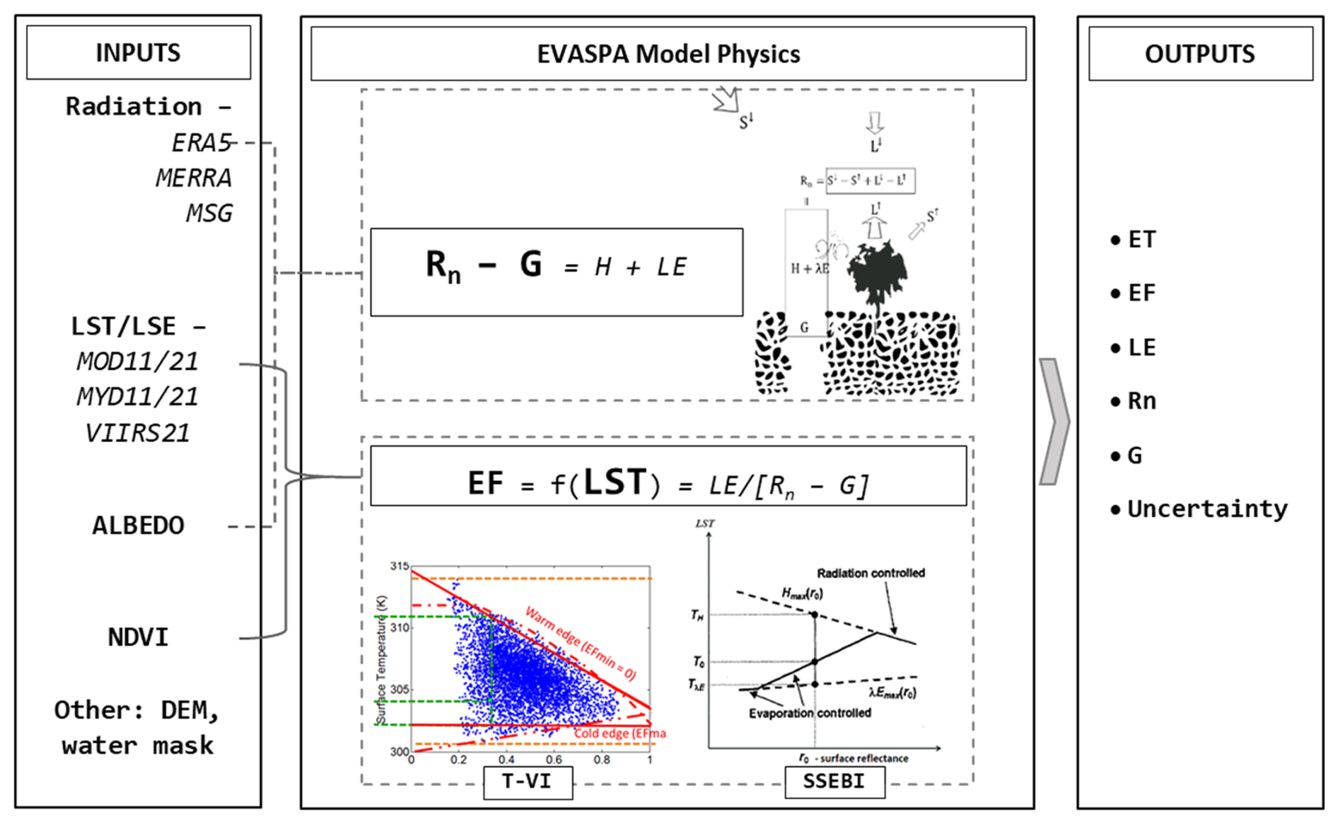
Figure 1 EVASPA system overview: inputs – e.g. from MODIS (aboard AQUA and TERRA satellites), VIIRS sensors; EF, SEB methods; and model outputs. The evaporative fraction (EF) and ground heat flux (G) methods used herein are summarized in Table A1.

2.1.3 Integration from instantaneous to daily ET and temporal interpolation for missing days

Eventually, the daily ET_d ($\mathit{\lambda }E/\mathit{\lambda }$) [mm d⁻¹] is computed using the daily solar radiation data, where it is commonly assumed that the λE-to-solar radiation ratio is conserved throughout the day, i.e. $\frac{\mathit{\lambda }{E}_{\mathrm{I}}}{{\text{SW}}_{\mathrm{I}}}\approx \frac{\mathit{\lambda }{E}_{\mathrm{d}}}{{\text{SW}}_{\mathrm{d}}}$ (e.g., Delogu et al., 2012). This allows for a straightforward integration/aggregation from instantaneous to daily ET values. While ensuring dimensional consistency, the area under the diurnal $\mathit{\lambda }{E}_{\mathrm{I}}/\mathit{\lambda }$ curve can be approximated as,

$$\begin{array}{}\text{(3)}& {\text{ET}}_{\mathrm{d}}={\displaystyle \frac{\mathit{\lambda }E}{\mathit{\lambda }}}={\displaystyle \frac{\mathit{\lambda }{E}_{\mathrm{I}}\cdot \frac{{\text{SW}}_{\mathrm{d}}}{{\text{SW}}_{\mathrm{I}}}\cdot \mathrm{86}\mathrm{400}}{\mathit{\lambda }}}\left[\mathrm{mm}{\mathrm{d}}^{-\mathrm{1}}\right]\end{array}$$

where λE_I [W m⁻²] is the instantaneous (at overpass) latent energy. λ [J kg⁻¹] is the latent heat of vaporization. SW_I [W m⁻²] and SW_d [W m⁻²] are the instantaneous and daily average shortwave radiation, respectively. SW_d⋅86 400 is thus the daily shortwave radiation.

It should be noted this is one of several methods used to aggregate latent heat fluxes to the daily scale. It was selected herein as it is physically based, requires minimal data and relatively simple to apply. We nonetheless acknowledge that it does introduce uncertainties in the estimations, especially since the assumption that the ratio is conserved throughout the day may not always hold. Within the TRISHNA SWEAT framework, other methods (e.g. conservation of the evaporative fraction throughout the day) are being tested to quantify such uncertainties between methods, and for possible inclusion as part of the product chain.

Temporal inter-/extrapolation: to ensure temporally continuous daily ET, an interpolation method using daily solar radiation (Allies et al., 2022; Delogu et al., 2012) was applied, where we rely on the continuous daily solar radiation data as a scaling variable. To reconstruct the daily ET for missing days, the ratio ${\text{ET}}_{\mathrm{d}}/{\text{SW}}_{\mathrm{d}}$ is computed for the periods when ET_d from EVASPA is available. The missing Λ_interp1 (equivalent to ${\text{ET}}_{\mathrm{d}\mathit{\_}\text{interp1}}/{\text{SW}}_{\mathrm{d}}$) estimates in the time series' are then gap-filled/interpolated by assuming a linear regression. The interpolated ratios (Λ_interp1) are then used together with the available SW_d (during periods with missing ET_d) to compute the gap-filled daily ET estimates as ${\text{ET}}_{\mathrm{d}\mathit{\_}\text{interp1}}={\mathrm{\Lambda }}_{\mathrm{interp}\mathrm{1}}\cdot {\text{SW}}_{\mathrm{d}}$. While this technique enables gap filling of ET datasets in a relatively simple manner, it possibly also introduces a potential source of error. In Sect. 4, we therefore also analyse/evaluate how this temporal interpolation step reduces or introduces further uncertainties in the final ET outputs.

2.2 Quantifying Uncertainty

The inherent differences in the theoretical assumptions (parameterizations, structure, physics, etc.) in ET models that have been proposed in the literature, together with the variability in input datasets used to drive such models results in a broad uncertainty in reported ETs (e.g., Jiménez et al., 2011; Etchanchu et al., 2025). As such, given the variability inherent in the input data and methods used to build the EVASPA ensemble (see Table A1: the EF, ground heat flux methods, and input data), uncertainties in the outputs are expected and should thus be quantified. Hereunder, our uncertainty analyses will mainly focus on latent [heat] and the corresponding ET [mass] fluxes, i.e., inter-comparisons and uncertainty between the ensemble ET members. We define the global uncertainty in terms of the standard deviation of all 972 EVASPA estimates (see Eq. 5c). This is then discriminated between the four variables (LSTs, radiation, EFs, G) for the specific uncertainty. To be consistent with recent ensemble ET products, which quantify uncertainty in SD, the TRISHNA ET products will also include the ensemble SD as the primary uncertainty measure (this may change as the products evolve). We nonetheless acknowledge that SD (and the corresponding coefficient of variation, CV) can be misleading, especially when the analysed data exhibits non-symmetrical (specifically non-Gaussian) distribution. As such, the coefficient of quartile variation or quartile coefficient of dispersion (QCD) – which was recommended for non-normal distributions by Bonett (2006) – has also been included as a complementary statistical measure of uncertainty in the EVASPA daily ET estimates. Note that ground daily ET observations are only used in the assessments as presented in Sect. 4.2.1 and are therefore not considered for uncertainty analyses, which are specifically meant to quantify the incertitude within the EVASPA ensemble.

2.2.1 Variability in input data

The MODIS sensor, carried on board the TERRA and AQUA satellites (with the respective products commonly denoted as MOD and MYD), acquires land surface emission data across four land-use thermal infrared channels, covering wavelengths ranging from approximately 8.4 to 13.5 µm (Wan and Li, 1997). The two satellites have distinct overpass times – TERRA in the morning and AQUA in the early afternoon – resulting in data acquisitions under differing radiative and surface energy exchange conditions. Consequently, the observed thermal signals from the surface are expected to exhibit noticeable differences between the two platforms, driven by the diurnal variations in temperature and solar radiation. Additionally, MODIS-derived land surface temperature and emissivity (LST/E) products for both satellites are generated using two primary retrieval algorithms: the Generalized Split-Window (GSW) technique and the Temperature-Emissivity Separation (TES) method. These products are denoted MxD11 and MxD21, respectively, where “MxD” here represents either MOD (for TERRA) or MYD (for AQUA). The fundamental differences in these algorithms – particularly in how they treat atmospheric correction and surface emissivity – can lead to notable discrepancies in the retrieved LST and emissivity values. Since LST is a key input in SEB modelling and directly influences the calculation of EF, such differences can propagate through the modelling framework and affect the resulting flux estimates.

For the radiation: (1) ERA5 (clear-sky) and ERA5-Land (all-sky) surface/single-level datasets are derived using the McRad scheme incorporating atmospheric conditions of the ECMWF Integrated Forecasting System (Morcrette et al., 2008). The hourly ERA5 and ERA5-Land analyses are produced globally at a spatial resolution of ∼ 25 and ∼ 9 km, respectively. (2) the 0.05° MSG radiation products are derived every 15 min from data acquired by the SEVIRI radiometer on board the geostationary Meteosat Second Generation (MSG) satellite, used together with the prevailing atmospheric information. (3) MERRA2 radiation data are derived using short- and long-wave parameterizations within the Goddard Earth Observation System-5 (GEOS-5) atmospheric general circulation model, yielding hourly data with a coarse spatial resolution of 0.5° × 0.625°. Although all three radiation datasets rely on similar algorithms to estimate the atmosphere's effective transmittance and emissivity, they exhibit large variations in their construction (e.g. discretization of the atmosphere) and thus characteristics.

To assess the significance of the variations in the LST and radiation inputs, we conducted a comparative analysis of the MxD11 and MxD21 LST/E datasets, and the estimated net radiations. In Sect. 4.1, we briefly present an overview of the observed variability in the LST and radiation products across the selected observation sites.

2.2.2 Uncertainty in the EVASPA estimates

Since the interpolation for days with missing satellite data relies on the method described in Sect. 2.1.3 – where the all-sky radiation data is the primary variable used to represent temporal trends of fluxes at the near-land surface – we analyse the non-interpolated and interpolated EVASPA ensemble members separately, while primarily focusing on AQUA and TERRA-based estimates. Due to the different timescale and issues with the VIIRS data (i.e. with the multiple view angle and overpass time zones within the images), the VIIRS-based analyses are summarised in the Supplement. Below, we present the uncertainties in the instantaneous and daily ensemble estimates prior to interpolation. The corresponding analyses after gap filling are discussed in Sect. 4.3.3. As interpolation is not applied to the instantaneous flux estimates – particularly the other surface energy balance components – that section specifically focuses on analysing the influence of the four variables on the daily ET estimates, where the radiation-based temporal interpolation is relevant and its effects can be assumed to be more pronounced.

2.3 Cluster Analysis and Performance Metrics

2.3.1 Similarity assessment: Cluster Analysis

To evaluate the similarity between the ET estimates at the sites of interest, as presented and discussed in Sect. 4.2.2, pairwise Euclidean distances (ED) between the members in the ensemble were calculated. The ED between member sets j and k in the EVASPA ensemble, ED_j,k, is defined as,

$$\begin{array}{}\text{(4)}& {\text{ED}}_{j,k}={\left(\sum _{i=\mathrm{1}}^N(Y_{i,j}-Y_{i,k}{)}^{\mathrm{2}}\right)}^{\mathrm{0.5}}\end{array}$$

where Y_i,j, Y_i,k are the modelled estimates for ensemble member sets j and k at time step i. N is the size of the time series.

These Euclidean distances were then visualized through dendrograms generated using the hierarchical clustering approach originally proposed by Ward (1963). Note that the rescaled EDs – rescaled relative to the maximum ED – are presented in the dendrograms (Figs. 8 and S3 in the Supplement). The analyses were independently conducted for each of the four distinct variables (i.e. LST, radiation, EF and G flux methods) in order to isolate and interpret their influence on the ensemble variability. For instance, in the case of the LST variable, hierarchical clustering was applied to ET estimates derived from each of the four LST products. This involved computing the Euclidean distance between all possible product pairs, resulting in six unique ⁴C₂ combinations; i.e. between estimates derived using MYD11 and MYD21, MYD11 and MOD11, MYD11 and MOD21, MYD21 and MOD11, MYD21 and MOD21, MOD11 and MOD21.

2.3.2 Performance assessment

For validation of the flux estimates against observations at the sites, we employed several metrics that quantify different aspects of model accuracy. Specifically, we used bias, mean absolute error (MAE), and root mean square difference/error (RMSD/E). In addition to these, we also computed Willmott's index of agreement (D), a dimensionless metric that consolidates the correspondence between predicted and observed values into a single value (Willmott, 1981). Willmott's D is particularly useful as it captures both systematic and unsystematic deviations by measuring both accuracy and precision, and thus provides a more integrated measure of model performance. As discussed in Sect. 2.2, we use standard deviation (SD), coefficient of variation (CV) and quartile coefficient of dispersion (QCD) to quantify the ensemble uncertainties (Sect. 4.3). These evaluation metrics are defined thusly,

$$\begin{array}{}\text{(5a)}& {\displaystyle }\begin{array}{rl}& \text{bias}={\sum }_{i=\mathrm{1}}^N(Y_i-X_i)/N;\\ & \text{MAE}={\sum }_{i=\mathrm{1}}^N\left|Y_i-X_i\right|/N;\\ & \text{RMSD}/E={\left({\sum }_{i=\mathrm{1}}^N(Y_i-X_i{)}^{\mathrm{2}}/N\right)}^{\mathrm{0.5}}\end{array}\text{(5b)}& {\displaystyle }D\left[\text{Willmott's\hspace{0.17em}\hspace{0.17em}index}\right]=\mathrm{1}-{\displaystyle \frac{{\sum }_{i=\mathrm{1}}^N(Y_i-X_i{)}^{\mathrm{2}}}{{\sum }_{i=\mathrm{1}}^N{\left(\left|Y_i-\stackrel{\mathrm{‾}}{X}\right|+\left|X_i-\stackrel{\mathrm{‾}}{X}\right|\right)}^{\mathrm{2}}}}\text{(5c)}& {\displaystyle }{\text{SD}}_i={\left({\sum }_{j=\mathrm{1}}^n(Y_{i,j}-{\mathit{\mu }}_i{)}^{\mathrm{2}}/n\right)}^{\mathrm{0.5}};{\text{CV}}_i={\text{SD}}_i/{\mathit{\mu }}_i\text{(5d)}& {\displaystyle }{\text{QCD}}_i=(Y_{Q\mathrm{3},i}-Y_{Q\mathrm{1},i})/(Y_{Q\mathrm{3},i}+Y_{Q\mathrm{1},i})\end{array}$$

Y and X represent the modelled estimates and the corresponding reference values, respectively. N denotes the size of the time series. μ and n in SD are the ensemble mean and ensemble size, respectively. Y_Q3,i and Y_Q3,i in the QCD are the respective first and third quartiles at ith time step.

For the accuracy assessments presented in Sect. 4.2.1, ground measurements/observations are used as the reference with the ensemble mean taken as the model estimate. Separately, in the heat-maps shown in uncertainty analyses sub-sections (see Sect. 4.3), each individual ensemble member within the EVASPA output array is, in turn, designated as the “reference”. Meaning one ensemble member is selected at a time to serve as the baseline against which all other members are compared. The resulting differences are then visualized to assess the consistency and variability across the entire ensemble, providing insights into the relative performance and agreement among the ensemble estimates.

3 Study area and input data

Table 1 summarizes the inputs used in this study. These include land surface temperature (from MODIS and VIIRS sensors), surface albedo, NDVI, LAI from MODIS. The MODIS/VIIRS products and MERRA radiation data over southern France were sourced from https://search.earthdata.nasa.gov (last access: 31 January 2026); with ERA5 and Meteosat Second Generation (MSG) radiations obtained from https://cds.climate.copernicus.eu (last access: 31 January 2026) and https://datalsasafwd.lsasvcs.ipma.pt (last access: 31 January 2026), respectively. Except for VIIRS, which starts in 2012, all other datasets were from 2004–2024. For ensemble members utilizing ERA5 radiation, the clear-sky data were used to derive the instantaneous estimates at the satellite's overtime, while the corresponding all-sky data from ERA5-Land were employed for aggregating to daily values and for performing the temporal interpolation. The contextual extents chosen for our calculations were: (a) South East France (green dotted box in Fig. 2): bottom-left (42.3° N, 2.4° E); top-right (44.5° N, 6.4° E), and (b) South West France (blue dotted box in Fig. 2): bottom-left (42.5° N, −1.75° W); top-right (45.25° N, 2.5° E). The two extents form the combined estimates over Southern France.

Table 1 Input data used to run the EVASPA SEB scheme (simulation period: 2004–2024). n/a: not applicable.

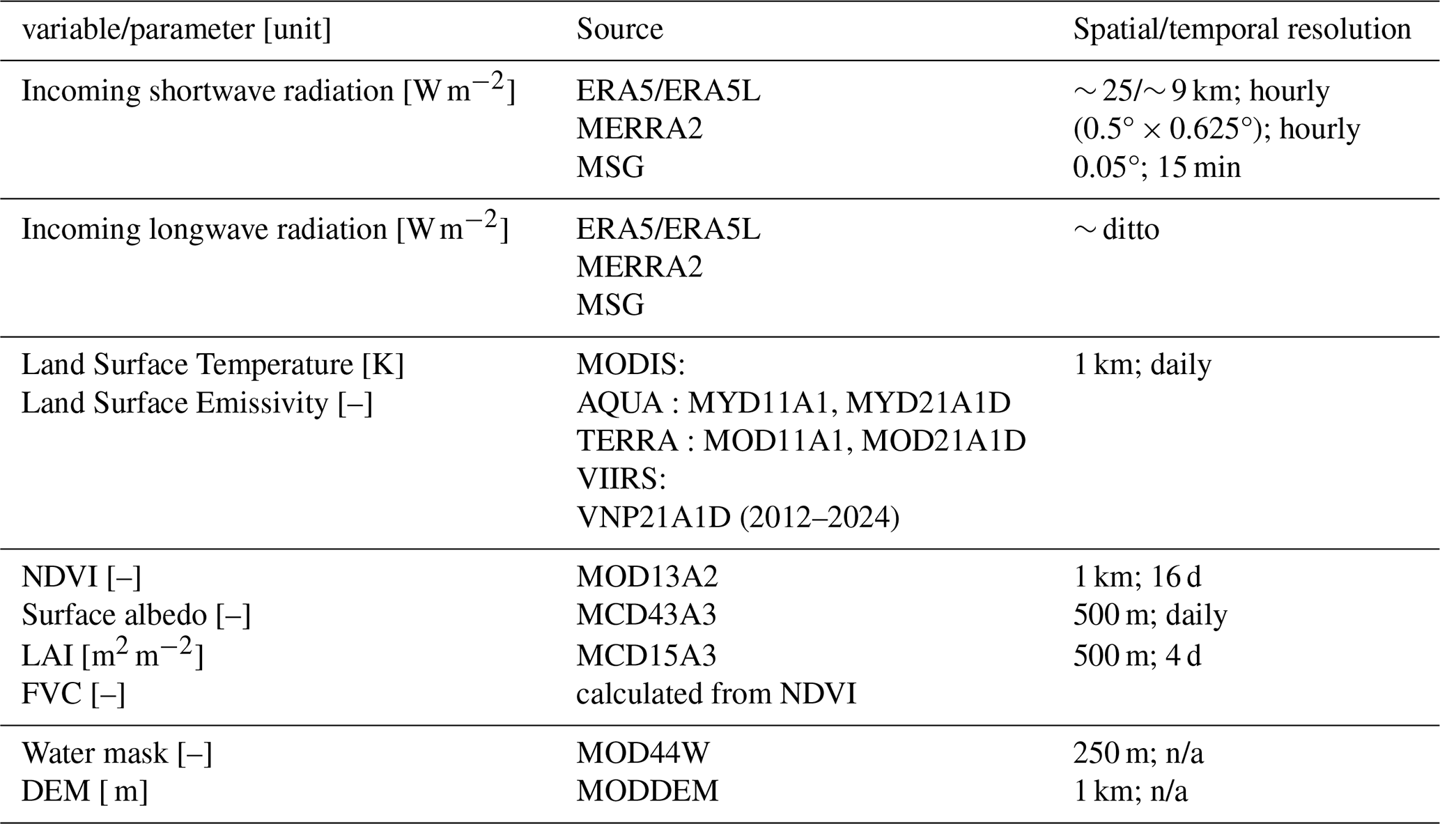
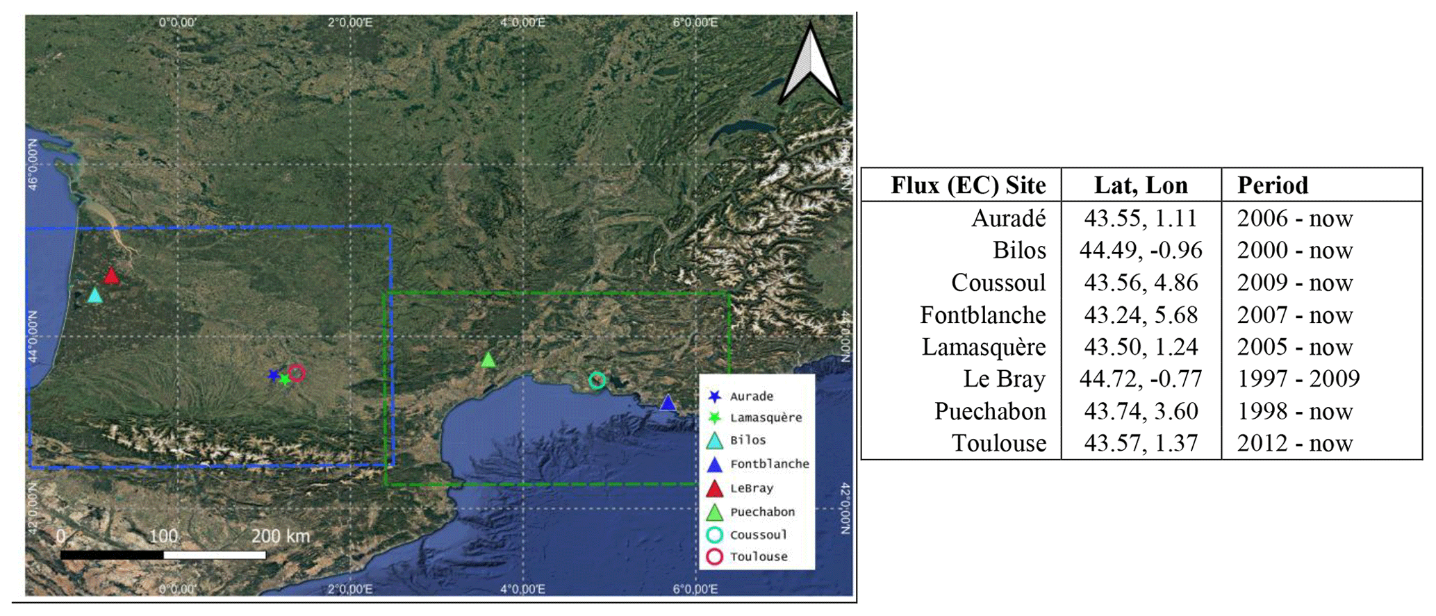
Figure 2 Contextual extents; and the sites in Southern France evaluated in this study – i.e. flux data observations over Δ Forests (4), ⋆ Croplands (2) and ∘ Grasslands (2). (Map data ©2024 Google). Right: the flux sites, coordinates and period.

Here, we report on AQUA- and TERRA-based analyses conducted across eight sites, whose spatial distribution over the southern region of France is shown in Fig. 2. A closer look at the VIIRS LST/E products (which have a different timescale versus MODIS, i.e. only start in 2012) revealed systematic issues related to viewing information. That is, view zenith angles (VZA) – see example in Fig. A1 where only edge VZAs (∼ 65°) are recorded when the VIIRS sensor is observing the pixel from the west, i.e. positive VZAs; and overpass times. These are likely due to the use of acquisitions from multiple orbit cycles to compile the VIIRS tiles, with such issues likely to propagate into the EF spaces and SEB calculations. Accordingly, the VIIRS-based EVASPA results are only briefly presented in the Supplement (Table S1).

To standardize the input data for analysis, we resampled the products with varying spatial resolutions to a uniform ∼ 1 km resolution using the nearest-neighbour approach, therefore ensuring compatibility with the native MODIS LST/E pixel. Pixels with missing values were not interpolated in space thus leaving them unchanged; this ensured the integrity of the available data (e.g. preservation of the EF feature spaces). For products not provided at a daily scale, such as the NDVI, we assumed that these variables remained constant over short periods. As such, the values were repeated across the acquisition interval – for instance, the 4 d LAI product was applied to days 5–8 by repeating the value from day 5. Pixels corresponding to water bodies were masked out and excluded from the evaporative fraction (and surface energy balance) calculations (note that only the cold pixels over land in the image are used to derive the wet edge). Additionally, the calculations of EF, and the subsequent SEB components and evapotranspiration were masked to a 300 m relief range, as determined by the MODIS digital elevation model (DEM) dataset. This masking was necessary to minimize potential errors introduced by lapse rate and slope effects on LST, thereby potentially improving the accuracy of the resulting EF estimates. The temporal variations in surface water bodies, as well as changes in surface elevation (from the DEM), were considered negligible and were, therefore, not accounted for in the analysis.

The daily ET flux observations (Fig. 2) were drawn from Fluxnet2015 (Pastorello et al., 2020), ICOS (ICOS-cp.eu, 2024), and other independent flux sites. The observation sites span different types of ecosystems including: (a) cropland (2), (b) grassland (2), and (c) forest (4) (see their geographical distribution in Fig. 2). The FLUXNET and ICOS datasets are gap filled using the research-standard Marginal Distribution Sampling (MDS) method, with the energy balance closure correction factor (EBC_CF, Pastorello et al., 2020) method, an adaptation of the Bowen ratio method, applied for SEB closure corrections.

4 Results and discussion

4.1 Evaluation of input data: Uncertainty in the radiation and LST inputs

4.1.1 Radiation (incoming shortwave and longwave)

Figure 3 illustrates the uncertainties associated with the radiation inputs for the sites mapped in Fig. 2, highlighting the variations and spreads that occur at the satellite overpass time. Notably, differences between the datasets become evident depending on whether the observations/analyses were made during the TERRA, AQUA or Suomi NPP (which carries the VIIRS sensor) satellite overpasses. The uncertainties in the incoming solar radiation, expressed as the standard deviation between the radiation values, appear to be more pronounced during the earlier morning hours – corresponding to the TERRA overpass – when solar angles are lower and incoming solar radiation is relatively lower. This increased variability is perhaps due to the enhanced atmospheric influence and the challenge of capturing accurate shortwave radiation under low sun angle conditions. In contrast, at the time of the AQUA overpass (and VIIRS to a similar extent) when incoming solar radiation tends to be higher due to the overhead sun position, the uncertainty in the solar radiation input is generally lower and more consistent across the radiation products. With respect to the incoming longwave radiation, values obtained from the three different radiation sources largely agree. The standard deviation (the absolute measure of uncertainty) remains relatively low across all three datasets, indicating limited divergence and suggesting higher confidence in the longwave radiation inputs compared to the shortwave components.

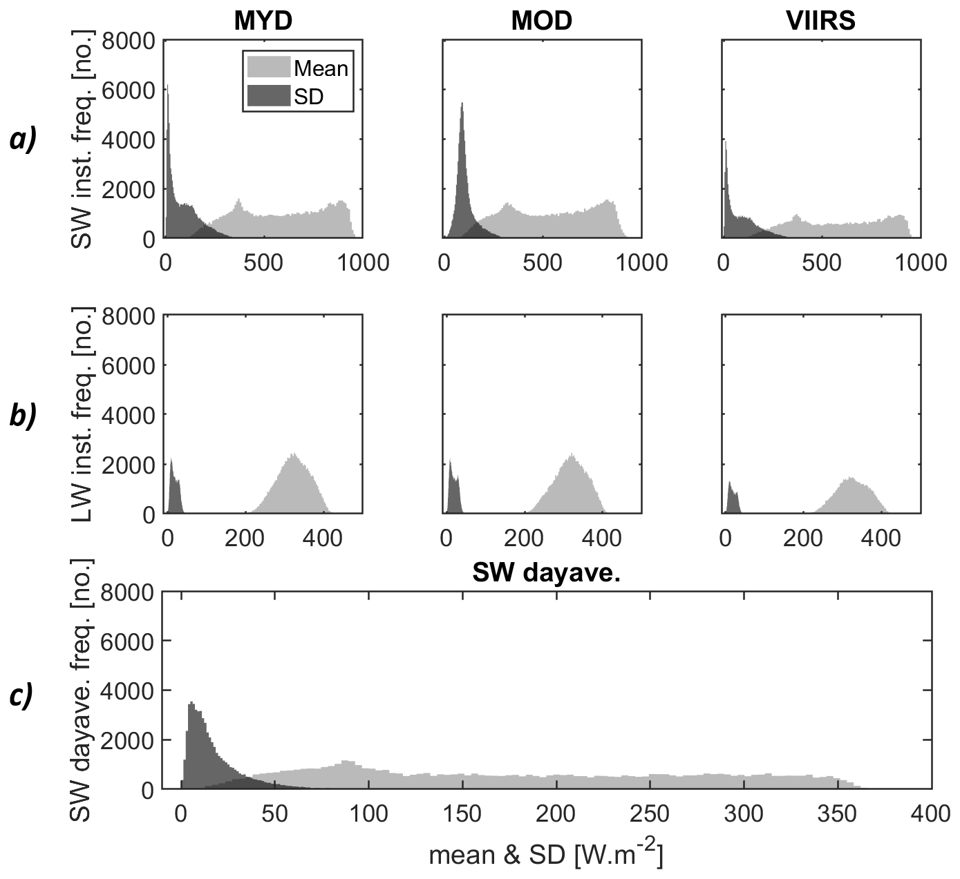
Figure 3 Global uncertainty in the radiation input data over the eight study sites – one pixel per site over the 2004–2024 study period. (a) Shortwave (SW) radiation  at the three unique satellite overpasses: i.e. AQUA (MYD), TERRA (MOD), and Suomi NPP (VIIRS), respectively; (b) same as (a) but for longwave (LW) radiation; (c) daily shortwave radiation – applies for all satellites/sensors.

4.1.2 Differences in LST/E by retrieval method and overpass time

To evaluate the significance of the variations above, we conducted a comparative analysis of the MxD11 and MxD21 LST/E datasets. In the following, we present a brief overview of the variability observed in these products across the selected observation sites.

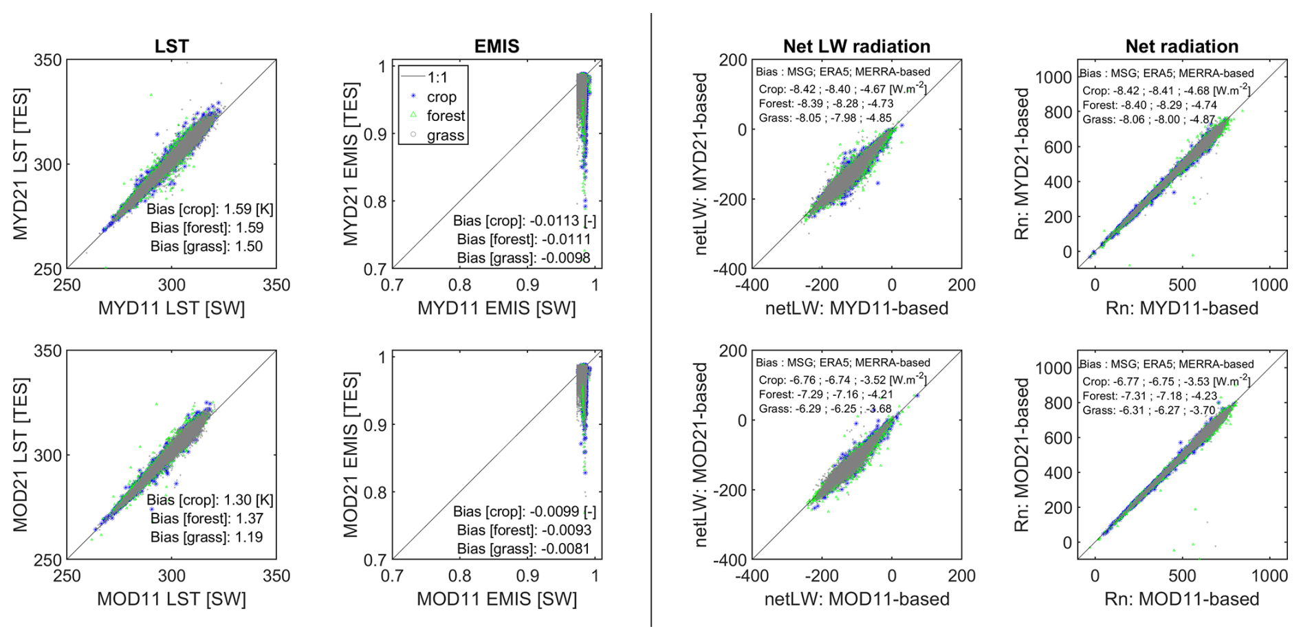
Figure 4 Scattergrams depicting the uncertainties in the LST/LSE, and in the net longwave radiation and net radiation computed therefrom. Left: TES (suffix 21) versus GSW (suffix 11) LST and LSE (top and bottom are MYD for AQUA and MOD for TERRA based values); right: net longwave radiation based on the MSG sky radiation (scatters are for net radiation calculated using MSG sky radiation; bias of the other sky radiations – ERA5, MERRA are included inset). VIIRS comparisons not shown as only the TES-based dataset, VIIRS21, is available.

As shown in Fig. 4, land surface temperature observations derived from the TES method (identified by MODIS product suffix “21”) tend to be systematically higher than those obtained using the GSW method, denoted by suffix “11”. This pattern is consistently observed across all land cover types evaluated in the study, though the magnitude of the bias varies. The most pronounced differences are seen over croplands and forested areas, where TES-derived LSTs exhibit the highest positive biases relative to the GSW-based estimates. Conversely, for emissivity retrievals, the trend is reversed: TES-derived emissivity values are generally lower than those from the GSW method. This is attributable to the constant emissivity range limit from the classification products applied within the GSW method. The bias in emissivity remains elevated over croplands, with smallest discrepancies observed over grasslands, suggesting that land cover type exerts some slight influence on the magnitude of the differences.

To investigate how these variations in LST and emissivity propagate into SEB components, we analysed their effect on both net longwave radiation and total net radiation, as shown in Fig. 4. The net longwave radiation is computed as LSE(R_LW−σLST⁴), while the net radiation is given by $R_{\mathrm{n}}=(\mathrm{1}-\mathit{\alpha })R_{\text{SW}}+\text{LSE}(R_{\text{LW}}-\mathit{\sigma }{\text{LST}}^{\mathrm{4}}$), where LSE is the surface emissivity, R_SW is the incoming shortwave radiation, R_LW the incoming longwave radiation from the atmosphere, LST is the surface temperature, σ the Stefan–Boltzmann constant, and α the surface albedo. Complementary to the LST, MxD21-based estimates of net longwave radiation are consistently lower than those from the generalized split window method. This is mostly attributable to the somewhat higher surface temperatures in the TES retrievals. Generally, the R_n shows a weak dependence on LST (thus net longwave radiation), which is theoretically expected; the largest share of R_n variability is mostly explained by the net shortwave radiation, underscoring its dominant role in driving the net radiative balance. However, despite these differences in inputs, the overall bias in both net longwave and net radiation remains relatively low. As such, their potential impact on SEB and subsequent ET estimations within the EVASPA framework is expected to be minimal. Perhaps, the timing of satellite overpass plays a more significant role in influencing SEB estimates than the specific LST/E retrieval algorithm applied, i.e., due to the inherently different surface, radiative and atmospheric conditions prevailing at each overpass time, which will tend to affect the radiative budget more directly than algorithm-specific differences. Additionally, the use of the varying LSTs is likely to introduce even larger variabilities to the evapotranspiration estimates particularly due to the primary role LST plays in the construction of the EF feature spaces for derivation of pixel evaporative fractions.

4.2 Performance and similarity assessment

4.2.1 Global and site-specific performance of daily ET estimates

Table 2 summarises the performance of individual EVASPA ET estimates – derived from the four AQUA/TERRA 11/21 LST products, three radiation inputs, nine EF formulations, and nine ground heat flux methods against ground-based measurements across the evaluation sites. Inter-comparisons of the estimates against those from AQUA 11 are also presented in Fig. 7. Separately, the performances per EVASPA member set are shown in Fig. 5. Given the differing timespans of MODIS (early 2000s) and VIIRS (post-2012), as well as known limitations in VIIRS LST data (e.g., view angle and overpass time effects), the VIIRS-based estimates are only briefly presented in Table S1.

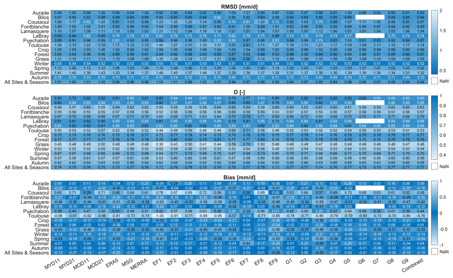
Figure 5 Performance heat maps (RMSD, D, and Bias) for the different EVASPA models across all evaluation sites. The EVASPA models are composed of all gap-filled member estimates in the set (e.g. the MYD11 set is constructed using the MYD11 LST/E data together with the 3 radiation datasets, 9 EF and 9 G methods). More details on how the sets are constructed are contained in Fig. S1 in the Supplements.

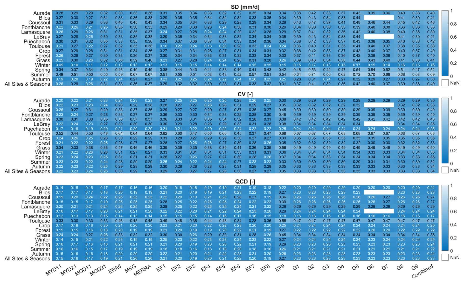
Figure 6 Uncertainty heat maps (median of SD, CV, and QCD over the study period) for the different EVASPA models across all evaluation sites. More details on how the sets are constructed are contained in Fig. S1.

Figure 7 (a) Scatter diagrams showing performance of EVASPA's daily ET estimates (the ensemble-average of temporally interpolated EVASPA members) against in-situ observations – (i) RMSD – vs. AQUA11 based and (ii) bias – vs. AQUA11 based. (b) Violin plots of RMSD, MAE, D index and Bias of all 972 EVASPA members per site and in all sites combined. Left side: the distributions, with the shaded area depicting the box plots (i.e. the interquartile range), the dot and horizontal line are, respective, mean and median of the performance metrics; right side: the histogram. The periods of observation vary per site but within the 2004–2024 simulation period.

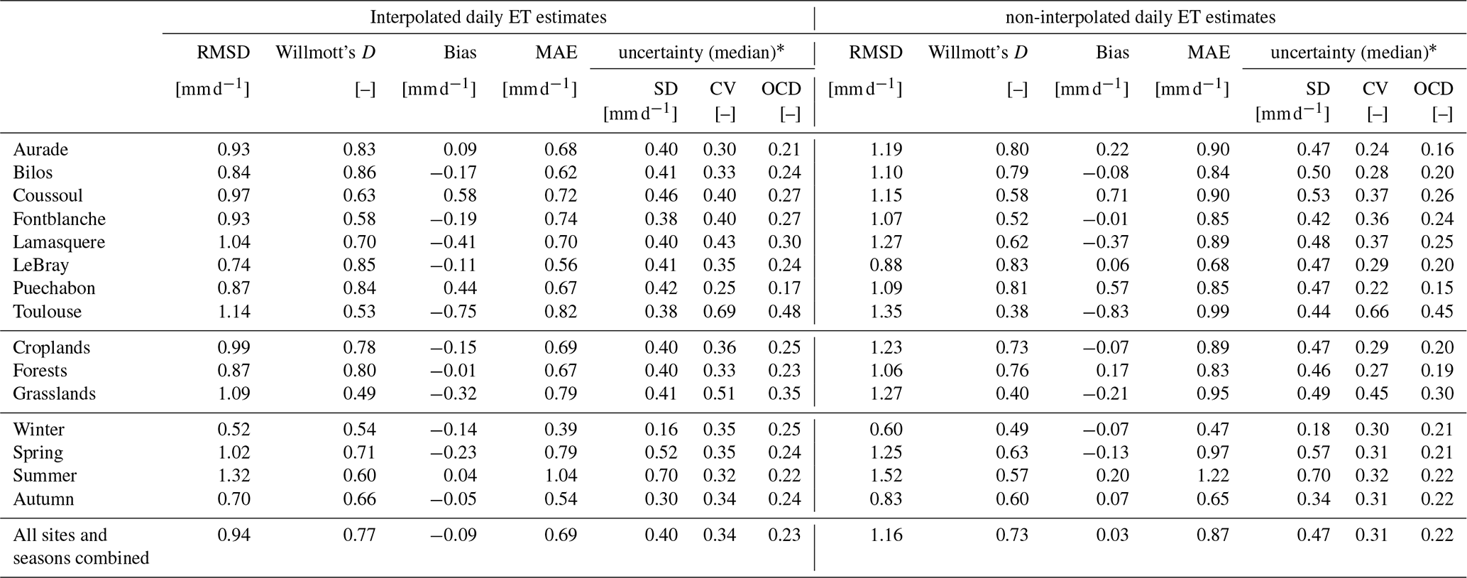
Across ensemble members, RMSDs ranged from approximately 0.7 to 1.6 mm d⁻¹, indicating variable but generally acceptable agreement with in-situ observations. Notably, the best performances were observed over forested sites, where the model appears to represent energy flux partitioning more accurately. In contrast, the least agreement (of all constituent EVASPA members versus the observations) was found in Toulouse, a grassland site situated within a built-up urban environment – suggesting that heterogeneous land surface conditions and urban interference may degrade retrieval accuracy. This is especially true when applying relatively coarse spatial data such as MODIS. In terms of bias (Fig. 7a), EVASPA tends to underestimate evapotranspiration fluxes over the relatively wet Toulouse site – again likely due to the heterogeneity within the MODIS pixel, specifically the presence of nearby built-up areas that typically exhibit higher LST and thus low evaporation rates. The relative uncertainty (see CV and QCD) within the ensemble is also highest at this site (Table 2, Fig. 6). Conversely, the model also seems to overestimate the ET fluxes at the other grassland site (Coussoul). Although this site is relatively homogeneous in land cover (and land use), it is located in close vicinity to some water ponds, which may interfere with the thermal signals captured at the pixel scale. This likely introduces noise that propagates through the modelling process influencing the final estimates. As expected, seasonal performance of daily ET across all EVASPA member sets is consistently driven by the availability of radiation used for the surface turbulent fluxes, with the best performance (in RMSD and MAE) observed in winter. The performance then cyclically degrades over spring through summer and improves into autumn (Table 2, Fig. 5). The absolute uncertainty (SD) in the estimated ensemble ETs shows a similar cyclical trend. The more informative relative uncertainty (as given by the relative SD or CV and the corresponding QCD) is however generally consistent throughout the seasons.

The interpolated daily ET estimates, gap-filled for missing days using daily average solar radiation information, demonstrate better performance compared to the uninterpolated ones. This is across all sites and for most performance metrics (i.e., all except a few cases where the bias is slightly increased), and shows the utility of radiation as a physically meaningful driver for estimating the temporal surface energy and water dynamics. Given its direct link to the surface available energy, solar radiation can be considered a good proxy for terrestrial energy (and thus water) exchanges, reinforcing its value in temporal reconstruction and modelling of ET in periods with incomplete input data/observations.

Table 2 Global performance of estimated daily evapotranspiration (average of all EVASPA ensemble members). Uncertainties within the ensemble are quantified using the median values of the standard deviation (SD), coefficient of variation (CV) and quartile coefficient of dispersion (QCD).

While the four LST datasets applied within EVASPA produced similar ET estimates across most sites (Figs. 5 and 7), subtle differences emerged between AQUA- and TERRA-based assessment results. These are likely attributable to diurnal variations in radiative and atmospheric conditions at the two satellite overpass times. Nonetheless, such differences tend to be averaged out at the daily scale, resulting in comparable overall performance between the two sets of daily ET (i.e., estimates based on AQUA and TERRA LST). At certain sites (most notably Toulouse), performance differences were more strongly tied to the temperature-emissivity separation method applied. There, the MxD21-based products (from both AQUA and TERRA) tended to yield better ET estimates than the corresponding GSW-based/11 products (Fig. 5, 3rd and 4th columns under Toulouse). This highlights the influence of LST/E retrieval methodology on subsequent surface energy balance calculations and, ultimately, on the accuracy of ET estimates. In terms of radiation, the MSG-based daily ET estimates appear to consistently outperform the MERRA- and ERA5-based estimates (see Fig. 5). This is perhaps due to the relatively higher spatial resolution of the MSG radiation data, which may better capture local-scale variability and thus improve representation of surface radiative conditions at the MODIS pixel scale.

In majority of the evaluated sites, the ensemble performance metrics (RMSD, MAE) exhibit either a Gaussian or positively skewed distribution, with the majority of members clustering close to the best performing model. In contrast, the performance in Toulouse appears bimodal (with a tendency towards negative skewness – see RMSD/MAE histogram in Fig. 7), suggesting the influence of at least two distinct sets of variables that contributing to the performance variability at the site. A closer inspection of the ensemble performance data at the site reveal that member estimates based on MxD21, particularly when combined with certain EF methods – most notably the T-VI approaches that incorporate edge refinement following Tang et al. (2010), dominate the best performing subset of the distribution.

Overall, the ensemble mean is shown to achieve better performance – especially in terms of RMSD – compared to majority of the member sets within the ensemble (see “Combined” versus other EVASPA sets in Fig. 5). This highlights the robustness and utility of ensemble frameworks, particularly in the modelling of earth processes where diverse methods/theories are often applied.

As the basis for the subsequent uncertainty decomposition analyses, we selected the MOD11/ERA5/EF7/G5 combination (Table A1), which exhibited performance close to the ensemble median in terms of RMSD across all sites. This allowed a stable reference for isolating the contributions of distinct variables to the overall model variability. For example, to investigate the specific impact of the EF methods on ET uncertainty, all estimates from the nine EF methods were applied in the SD calculations while selecting MOD11, ERA5 radiation and the G5 soil heat flux method (see Table A1). This design ensured that the captured variability was primarily attributable to the different/independent variables. Nonetheless, the overall trends remained largely consistent, even when different reference combinations of the distinct variables were used (see Fig. 12).

4.2.2 Similarity assessment of the EVASPA ensemble daily ET estimates

Overall, the similarity order between the EVASPA members for both the un-interpolated and gap filled EVASPA estimates appears identical (Fig. 8). The LST-based estimates are clustered/grouped according to the temperature separation methods, with the dissimilarity or variability between the daily ETs mostly arising due to the two (AQUA, TERRA) overpasses. For the EF and G-based evapotranspiration estimates, the similarity clustering is mostly according to the biophysical variable applied (i.e. albedo, NDVI for EFs, and NDVI, LAI, FVC for the G flux methods, respectively). The flat edge EF methods – EF3 (LST-albedo) and EF8 (LST-NDVI) – show the highest similarity while also appearing to have better agreement with the other S-SEBI/albedo based EFs. After interpolation, the similarity between the radiation-based ETs increases (reduced ED). The reduced spread/variability (see SD in Fig. 3c) between the daily shortwave/solar radiation datasets, which are used for gapfilling, likely contributes to this enhanced similarity, Conversely, the similarity based on the other variables – LST, EF and G – appears to reduce (increased ED), albeit marginally. This degraded similarity can be ascribed to the variability inherent in the additional (gap-filled) data points used for deriving the ED. Overall, compared to those from the G-based estimates, the absolute Euclidean distances between the LST-, EF- and the Radiation-based ET estimates are generally higher for all pair combinations, confirming the ensemble variability (thus uncertainty) observed in the following sections.

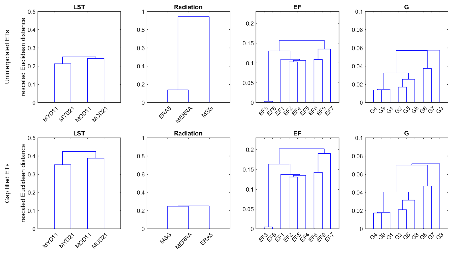
Figure 8 Dendrograms of the similarity between the ensemble ET estimates (based on the Euclidean distance between pairs of members in the ensemble). Similarity is assessed and discriminated according to the four distinct variables: LST, Radiation, EF methods and G flux methods (see variables list in Table A1). Evaporative fraction methods are – S-SEBI: EF1-EF5 and T-VI: EF6-EF9. G flux methods are – NDVI based: G1–G4; FVC based: G5; LAI based: G6–G7; and based on the LAI calculated from NDVI: G8–G9. Top – non-interpolated estimates; and bottom – interpolated/gap filled estimates. The ordinate is the rescaled Euclidean distance (ED) between the distinct member sets in the ensemble (for easier interpretation, varying y-limits are used for the distinct variable sets but similar for the non-interpolated and gap-filled estimates).

The similarity diagrams in the ensemble including the VIIRS based estimates (see Fig. S3) generally resemble those without VIIRS illustrated above in Fig. 8. However, for the LST analyses, the VIIRS based estimates exhibit the largest dissimilarity with the TERRA and AQUA based estimates.

4.3 Uncertainty in flux estimates due to LST, Radiation, EF and G

4.3.1 Instantaneous energy flux estimates: prior to temporal interpolation for missing days

Comparisons of the variability within EVASPA ensemble members are shown in the heat maps in Fig. 9. The heat maps are presented separately for the different instantaneous SEB components (net radiation, ground heat flux, latent heat flux and evaporative fraction). Despite the relatively good 1:1 agreement (see Willmott's D index), differences (in absolute terms as given by the MAE) are apparent in the estimated net radiation (R_n) components. These descripancies can somewhat be attributed to the product's overpass characteristics used in the calculations – particularly for the R_n derived from the ERA5 radiation inputs when the TERRA based LST/E products are used for estimating the surface emission. Conversely, while the agreement between other G estimates with those derived from LAI appears weaker, the absolute values remain largely comparable (see MAE under G). The available energy (R_n−G) that is partitioned into turbulent fluxes therefore follows a similar trend as R_n. The D index for EF estimates also show some degradation, with the MAE values exhibiting larger variations depending on the LST applied in the EF spaces. As a result, variability in latent heat flux estimates resembles that of EF, with additional influence introduced by the incertitude in radiation. Notably, large absolute differences (i.e. MAE > 0.2 [–]) can be observed between the EFs across overpass times – irrespective of the temperature emissivity separation method. This suggests that the common assumption of EF conservation throughout the day may not always be valid.

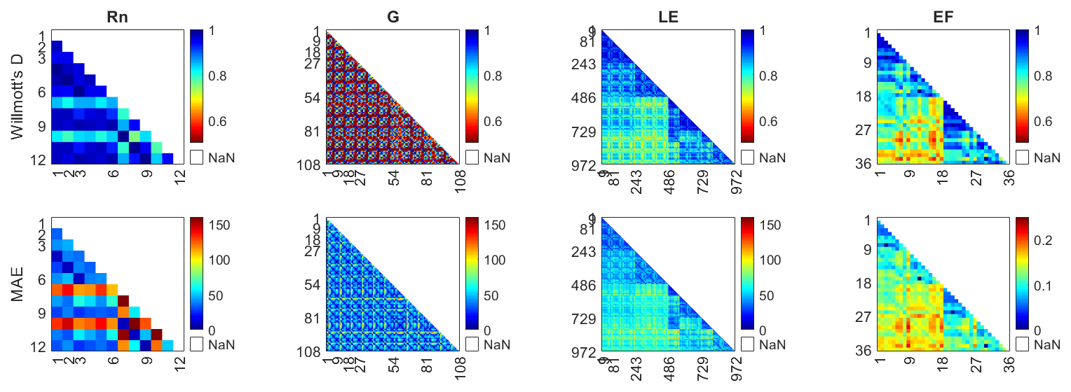
Figure 9 Heat maps of Willmott's D index [–] and MAE [W m⁻²] (or MAE [–] for EF) between the EVASPA SEB members (net radiation – R_n, ground heat flux – G, latent heat flux – LE, and evaporative fraction – EF) over all sites and seasons combined. Heat maps of the metrics are calculated by taking each individual member vs. all other ensemble members. Fluxes (R_n, G, LE) were here rescaled for consistent comparisons between overpasses. ^∗ Numbering in the heatmaps/ensemble is done according to the list of variables given in Table A1. E.g. for EF: 1–9 – all 9 EF methods/spaces using MYD11 LST, 10–18 – all EF methods/spaces using MYD21 LST, 19–27 – all EFs using MOD11 LST, and 28–36 – all EFs using MOD21 LST. ${}^{\ast \ast }$ Distinct number of variable combinations in the heat maps are given in Table A1. ${}^{\ast \ast }$ I.e., net radiation – 3 × 4 combinations (radiation × LST products); G flux – 9 × 3 × 4 (G methods × radiation × LST products); LE fluxes involve 9 × 9 × 3 × 4 combinations (G methods × EF methods × radiation × LST products); EFs – 9 × 4 combinations (EF methods × LST products).

The heat maps corresponding to the different land covers and seasons are presented in the Supplement. Across the land covers, the trends are generally similar to those in Fig. 9 with only subtle differences (Fig. S4). In contrast, seasonal patterns show more pronounced variability, particularly in estimates of the net radiation and latent heat flux terms. During winter, the larger variability in net radiation members appears to propagate into the latent fluxes. This leads to comparable variability as depicted in the seasonal net radiation and latent heat flux heat maps. In summer, despite even larger differences the net radiation, its effect on latent flux estimates is muted, with EF variability becoming more dominant. A similar trend is observed in spring and autumn where EF values from the different evaporative fraction methods and LST products exert the primary influence on latent energy.

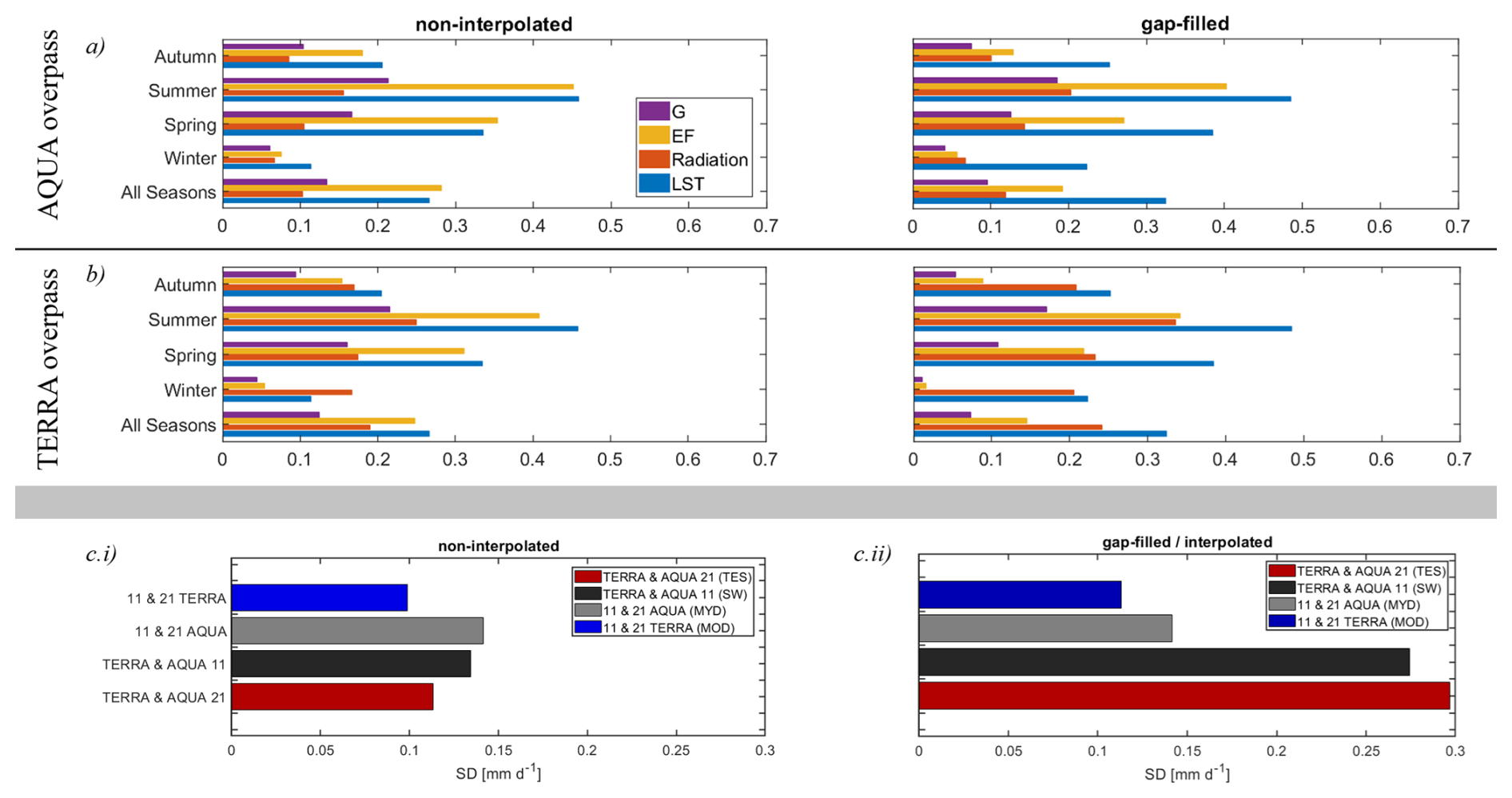
Figure 10 Bar graphs of standard deviation (SD) between the separate EVASPA ET estimates over the 2004–2024 study period, i.e., the specific uncertainty for all four distinct variables (across all sites combined). (a) At AQUA overpass – without and with gap filling/temporal interpolation. (b) At TERRA overpass – without and with gap filling/temporal interpolation. (c) For the 4 LSTs (separately between 11 and 21 for TERRA, between 11 and 21 for AQUA, between AQUA and TERRA for 11, between AQUA and TERRA for 21) – (c(i)) based on non-interpolated estimates, (c(ii)) based on interpolated estimates.

4.3.2 Non-interpolated daily ET estimates

Compared to the TES LST/E separation, the GSW method appears to introduce more variability (in absolute terms) among the ET ensemble members. This is evident in the standard deviation plots (Fig. 10c(i)), where GSW-based LST/E estimates generally diverge more strongly than those from TES. This likely reflects retrieval uncertainties tied to land cover classification products used to constrain emissivity ranges. Interestingly, when temporal interpolation is applied using radiation data to gap-fill missing days, this trend reverses. Here, the GSW based estimates exhibit lower uncertainties compared to the TES based estimates. This reversal suggests that interpolation stabilizes GSW retrievals by leveraging radiation trends, thus highlighting the complex interaction between retrieval approaches and gap-filling methods in shaping the ensemble ET uncertainty. Nevertheless, while the TES versus GSW distinction does contribute to the ensemble spread, the use of LST/E observations acquired at different satellite overpass times appears to be another source of uncertainty. For the non-interpolated estimates, the acquisition time has some influence. However, the greater influence due to overpass time comes after gap filling (see Figs. 10a, b and A2), and can thus be ascribed to the data and/or method used for temporal interpolation. Even though the differences between estimates derived from TERRA (morning) and AQUA (afternoon) appeared larger than those caused by temperature retrieval methods, the analysis on non-interpolated estimates could not lead to fully conclusive interpretations.

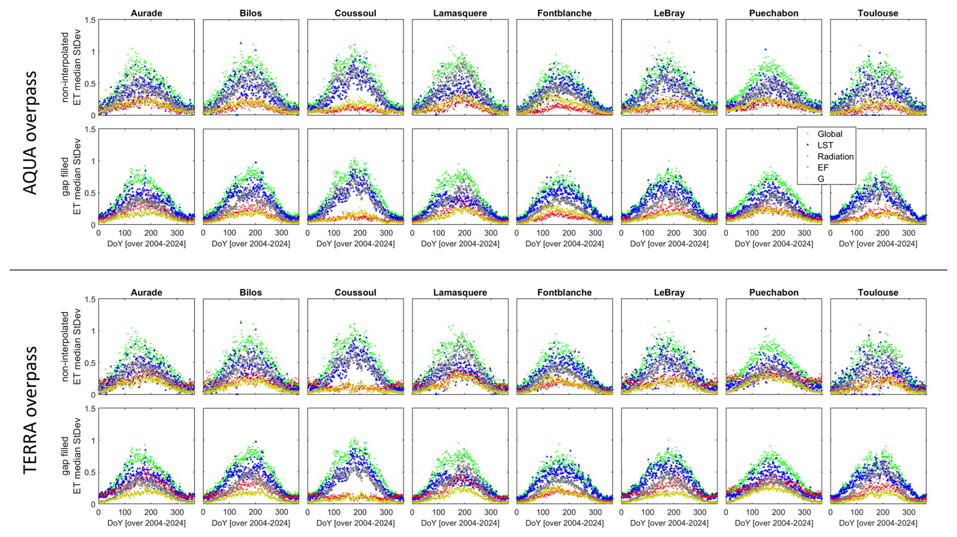
Figure 11 Time series' of specific and global uncertainties in the daily ET estimates. That is, the median SD for all days over the 2004–2024 simulation period. Separately for: (a) non-interpolated and gap filled estimates at AQUA's overpass; (b) non-interpolated and gap filled estimates at TERRA's overpass.

Figure 11 presents the evolution of the global and specific uncertainties (i.e. median SD) across the sites over the 2004–2024 study period. The LST-specific uncertainty curves are identical for both overpasses (as all four LST-based estimates are used in deriving the SD), but they differ between non-interpolated and gap-filled cases. Cross-site uncertainties are systematically higher during TERRA's winter overpasses (December–February) compared to AQUA's, indicating seasonal variations in input consistency that affect ET spread. The elevated winter uncertainties during TERRA's earlier overpass likely reflect low solar angles, which exacerbate inconsistencies in radiation products (see Sect. 4.1.1). By contrast, non-winter periods and AQUA overpasses show greater radiation product consistency, hence lowering their influence on ET uncertainty. Under these conditions, radiation inputs rank below ground heat flux methods among the drivers of daily ET uncertainty. This points to a seasonal shift in dominant uncertainty sources, linked to the Sun–Earth geometry and atmospheric conditions – particularly evident in the uninterpolated ensemble estimates.

Of the four variables examined, variations linked to evaporative fraction methods consistently ranked as the second largest source of uncertainty in the EVASPA estimates, ranking just below LST. This trend holds across sites and time periods (except at TERRA's overpass during winter). This indicates that while EF method selection does not introduce the highest uncertainty, it still plays a significant and persistent role in the global variability of the estimates. The stable ranking highlights the need for careful EF method selection, particularly in terrestrial applications where moderate levels of sensitivity to modelling assumptions can impact the reliability and accuracy of evapotranspiration estimates.

Figure 12 shows the specific uncertainties assigned to the four distinct variables while changing the reference combination (i.e. MYD11, ERA5, EF7, G5) used in majority of the incertitude calculations. Only the bar graphs for all sites combined are shown – the site-specific graphs show a similar trend (see Fig. A2). From the plots, the overall trends (particularly on ranking of the four variables) appeared largely similar across the analyses, even when alternative reference combinations of the distinct variables were considered. This suggests that the observed patterns are largely consistent and not overly sensitive to the specific choice of reference inputs-methods combination. LST still appears to introduce most of the overall (all seasons) uncertainty over the three land covers (see Figs. S6–S8). Nonetheless, the salience of EF methods on the uncertainty over the grasslands and croplands is apparent, especially in the non-interpolated daily ET estimates during summer.

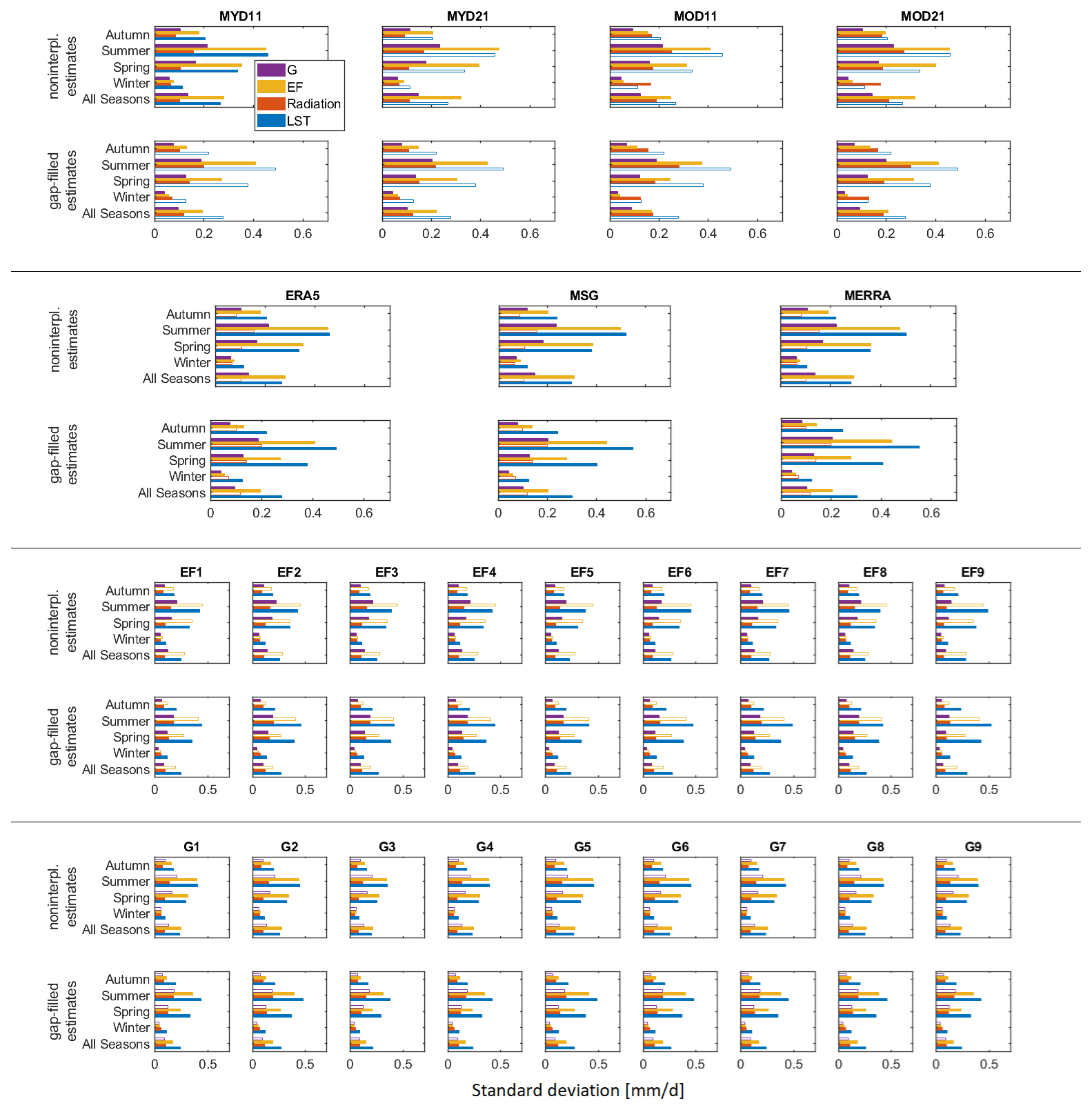
Figure 12 Standard deviation (median) bar graphs of the specific uncertainty introduced by selecting different member combinations of LST-Radiation-EF-G over the 2004–2024 simulation period.

4.3.3 Uncertainty in gap filled daily ET estimates and influence of the temporal interpolation method

To recall, missing days in the EVASPA ET time series' were gap filled using an interpolation method that exploits the temporal dynamics in continuous radiation data (see Sect. 2.1.3). Since the radiation input datasets have inherent uncertainties as presented in Sect. 4.1.1, it is reasonable to expect that such could indeed influence the resulting ensemble ETs. Figure 10a and b illustrate the uncertainties in the interpolated ET estimates (and the respective SDs in the non-interpolated ETs for comparison) over all sites combined and seasons. The graphs for each separate site are shown in Fig. A2. When the radiation datasets are relatively consistent, i.e. at AQUA's overpass time, the impact of the flux interpolation is comparatively muted. In such cases, radiation variables still contribute to the overall uncertainty but rank third, behind the LST inputs and EF methods. Contrarily, at TERRA's overpass, when the radiation datasets exhibit greater variability – particularly under challenging conditions such as low solar angles and generally low visibility during winter – the influence of radiations on the simulated ETs becomes more pronounced. Here, radiation input variables sometimes surpass EF methods in their contribution to ensemble uncertainty, ranking second behind LST.

Examining the uninterpolated estimates in Sect. 4.3.2 (see also Figs. 10 and 11), we observed that the ground heat flux tends to occasionally introduce greater uncertainty (particularly during AQUA's overpass and in non-winter periods) surpassing the radiation inputs as a source of variability in the simulations. For the gap filled estimates, however, the variability inherent in the radiation products becomes more prominent, even during periods typically associated with greater stability – such as at AQUA's overpass. Despite the relatively better consistency between the radiation datasets at these times, their influence on the interpolation process is amplified, perhaps due to their primary role in filling temporal gaps. As a result, the uncertainties introduced on the outputs by the radiation inputs start to outweigh those associated with the ground heat flux methods (see the “All Sites”, “All Seasons” bar graphs in Fig. 10a and b).

Specifically looking at the LST/E products, we observed that the overpass time tended to yield significant variability in the gap-filled daily ET estimates compared to the temperature emissivity separation methods. This is likely due to diurnal variability in LST and radiative fluxes, which are highly sensitive to the timing of observation. The overpass time determines the prevailing solar radiation, atmospheric characteristics, and surface/radiative energy partitioning, all of which largely influence the SEB and evaporative fluxes. Indeed, the uncertainty introduced by the two temperature separation methods at each acquisition show a tendency to remain the same for both the non-interpolated and gap filled daily ET estimates (see Fig. 10c). This is because the radiation used for interpolation is the same for each set – for example, the radiation used to interpolate the estimates based on MYD11 and MYD21 LST/Es is the same (i.e. at AQUA's overpass time), similarly for the TERRA based set. Conversely, two sets of radiation datasets are required to interpolate the MYD11 and MOD11 (similarly MYD21 and MOD21) estimates, depending on the acquisition time. These uncertainties propagate during interpolation resulting in the increased SD between AQUA and TERRA based estimates.

5 Summary and conclusions

In this study, we applied remote sensing data over the south of France to investigate the sources of uncertainty in long-term contextual modelling of ET, with initial model assessments performed using in-situ ET fluxes observed over eight sites. Our primary objective was to identify how different input datasets and methodological assumptions affect the variability and reliability of satellite-derived ET estimates. To this end, we used the ensemble-based EVASPA scheme – a tool that generates estimates of surface energy balance (SEB) components, including latent heat flux used as a basis for ET. The tool was implemented in a multi-data, multi-method setup, involving five LST/E products (four from MODIS, one from VIIRS), three radiation products (ERA5, MERRA, MSG), nine evaporative fraction methods (based on T-VI and S-SEBI), and nine ground heat flux methods (informed by NDVI, LAI, and FVC). This comprehensive setup allowed us to systematically assess where uncertainties emerge and how they propagate through the ET modelling workflow.

Practically, our findings suggest that:

• a.

  Even when using a simple ensemble average, performance over the long-term is generally reasonable across all sites. However, agreement appears to diminish especially over heterogeneous pixels. Performance of the individual member estimates within the ensemble also varies significantly, with the different constituent input and methods showing varying performance depending on the site. For example, the TES-derived LSTs appear to consistently outperform the GSW-derived LSTs over the Toulouse grassland site. As expected, the absolute seasonal performance (i.e. RMSD, MAE) is primarily influenced by the availability of radiation.

• b.

  Of all the four considered variables, the LST inputs introduce the largest spread (thus uncertainty in terms of SD) in the EVASPA ETs, followed by the EF methods and the radiation products, with the ground heat flux methods – G – having the least influence. This highlights the key role of LST and EF methods in determining:

  • –

    The available energy (R_n−G) at the near-land surface (where LST is a key input term for the net radiation, R_n).

  • –

    How this available energy is partitioned between the turbulent heat fluxes in contextual modelling of ET, i.e., when deriving the evaporative fraction at the pixel scale.

  While the differences in temperature-emissivity separation methods impact the agreement between ensemble members, the temporal aspect of LST/E acquisition introduces a broader and more systematic influence on ET uncertainty. This is primarily due to the associated variability in the radiation inputs at those times. For applications requiring high precision or sensitivity to temporal dynamics (for example, crop stress monitoring or irrigation scheduling), these timing effects may need to be accounted for explicitly, either through ensemble weighting strategies or temporal normalization approaches. Future ET modelling efforts may benefit from leveraging terrestrial emission data from missions with higher revisits or temporal frequency. This could minimize the uncertainty associated with use of data acquired at multiple times.

  It should nevertheless be noted that the uncertainty in ensemble-based modelling (particularly the global uncertainty, where all methods are combined) could be lower when compared to analyses including variations of additional factors, such as albedo estimation algorithms, additional evaporative fraction methods applying more complex edge detection algorithms, or a larger range of input data (see Olioso et al., 2023). These aspects, in addition to the directional influence of LSTs acquired from low elevation angles on the ETs (as is apparent in point SEB; Mwangi et al., 2023a, b), are to be explored in the near future.

Whereas this study is generally appropriate for site-based uncertainty assessments, we also acknowledge that several spatial scale issues exist that limit spatial generalization and transferability of the results. In particular, there is a clear scale mismatch between the estimates derived from (and for) the MODIS pixel, which represent relatively large and heterogeneous spatial areas, and the in-situ observations, which are representative only of the localized EC flux tower footprint. As such, the performance assessment results should be interpreted with caution, as the comparison involves estimates and observations with fundamentally different spatial coverage and representativeness. This limitation is further compounded by the presence of mixed pixels, where multiple land cover types and surface characteristics are aggregated within a single pixel, introducing additional uncertainty that is not explicitly accounted for in our analyses.

Being among the initial steps in defining an algorithm that will provide continuous ET estimates and the corresponding uncertainties on a pixel basis, this study aims to contribute to the definition of the operational evapotranspiration product for the TRISHNA mission. The work underscores the importance of both spatial and temporal resolution in the remote sensing of ET and associated near-land surface energy fluxes. In particular, the sensitivity of ET estimates to satellite overpass time highlights a fundamental limitation of current LST acquisitions, which often capture land surface conditions at diverse times diurnally. Future missions should prioritise higher temporal resolution in addition to improved spatial scales, especially for applications in agro-hydrology and land surface modelling where rapid surface changes contribute in driving the water and energy budgets. Together with TRISHNA, other emerging missions such as, LSTM, and SBG represent significant progress in this direction. These missions will offer the potential for high-resolution thermal observations with shorter revisit times, especially if the fusion of observations across missions/platforms is enabled. In addition to spatio-temporal improvements in satellite instruments, there is also a need for standardized processing protocols and ensemble modelling frameworks. Our findings highlight the relevance of ensemble-based approaches (such as EVASPA), which can incorporate multiple datasets and methods to characterize uncertainty and thus improve ET estimation accuracy, while also enhancing the resilience of Earth observation products.

Appendix A

EVASPA ensemble: inputs and methods

Herein, we use different LST and radiation input datasets. These are used to drive the EVASPA algorithm while utilizing different formulations of evaporative fraction and ground heat flux methods. These are as tabulated below.

Table A1 Ensemble construction: inputs – LST, Radiation; methods – EF (for wet and dry edge determination) and G flux functions used in this study.

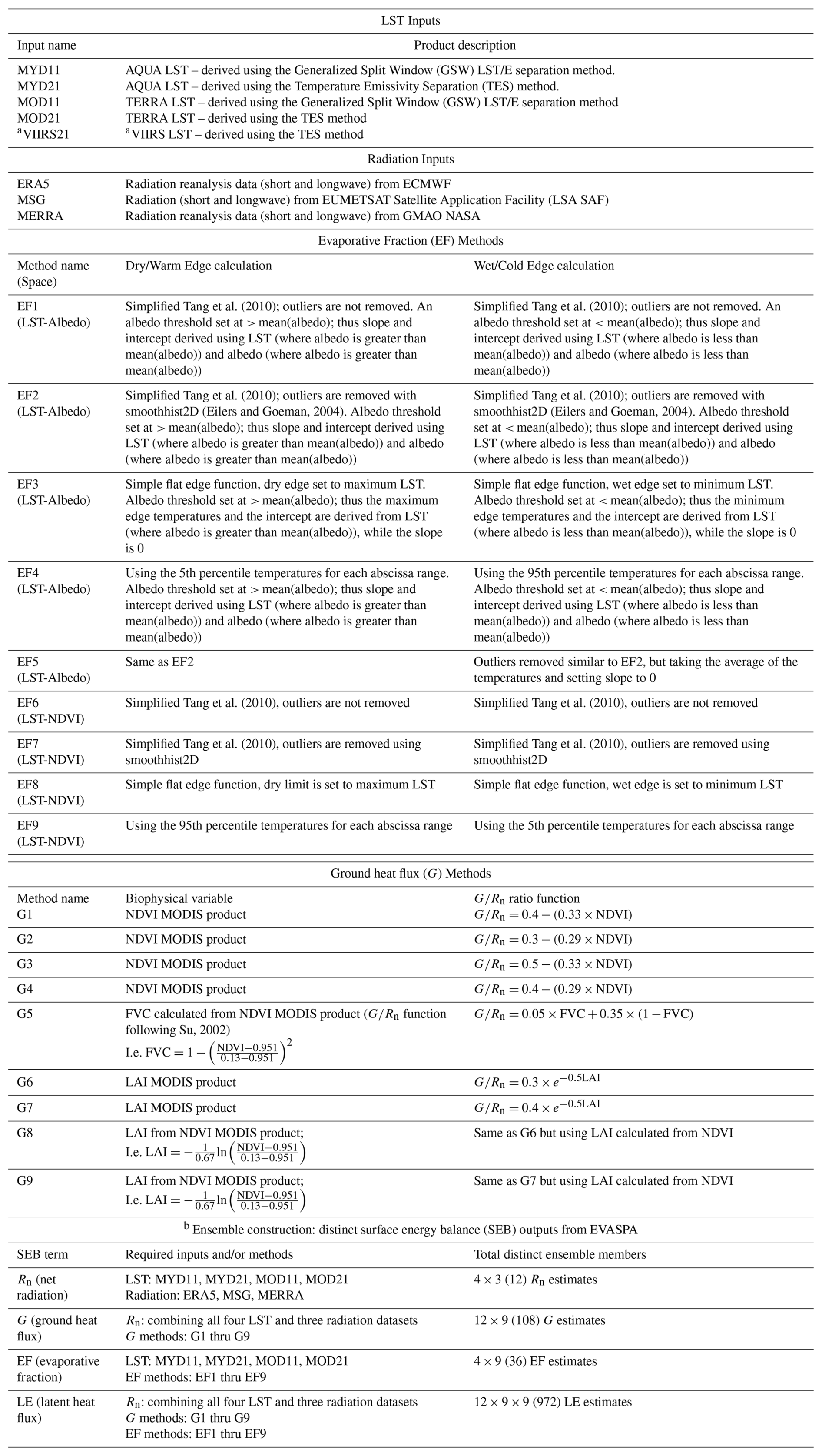
^a VIIRS21-based results mostly presented in the Supplement. For consistency, main text mainly focuses on EVASPA estimates based on AQUA and TERRA LSTs. ^b As in the main text where only AQUA and TERRA LST data are applied.

A1 Viewing information of AQUA, TERRA and VIIRS platforms

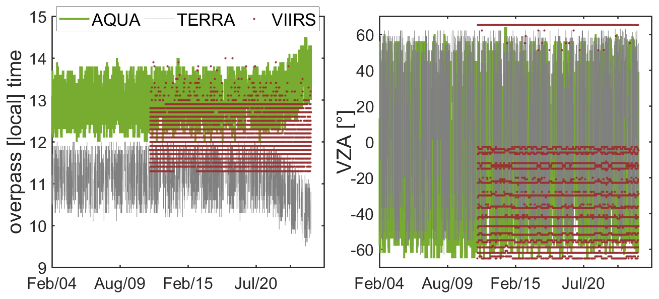
Figure A1 (Left) the overpass time (showing the effects of the orbit drift in the AQUA and TERRA satellites from mid/late 2020), and (right) view angle (showing possible issues with the VIIRS sensor when viewing from the west) over the 2004–2024 period. View information is drawn from a MODIS/VIIRS pixel in the South East AOI.

A2 Uncertainties in daily ET per site

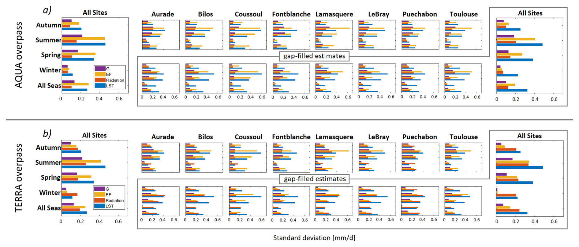
Figure A2 Bar graphs of standard deviation (SD) between the separate EVASPA ET estimates over the 2004–2024 simulation period. I.e., the specific uncertainty for all four distinct variables (across all sites combined and individually) at: (a) AQUA overpass – without and with gap filling/temporal interpolation; (b) TERRA overpass – without and with gap filling/temporal interpolation.