Comparison of ensemble assimilation methods in a hydrological model dedicated to agricultural best management practices

Hydrological models are valuable tools for understanding the movement of water and contaminants in agricultural catchments. They are particularly useful for assessing the impact of landscape organization on pesticide transfers and for developing effective mitigation strategies. However, using these models in an operational context requires reducing uncertainties in their outputs, which can be achieved through data assimilation methods. In this study, we aim to integrate surface moisture images into the PESticide and Hydrology Modelling at the catchment scale (PESHMELBA) water and pesticide transfer model using data assimilation techniques. Twin experiments are conducted on a virtual catchment consisting of vineyard plots and vegetative filter strips. We compare the performance of the ensemble Kalman filter (EnKF), the ensemble smoother with multiple data assimilation (ES-MDA), and the iterative ensemble Kalman smoother (iEnKS) in jointly estimating vertical moisture profiles and van Genuchten soil water retention properties of all soil horizons. Results indicate that the ES-MDA performs the best in estimating surface moisture and saturated water contents, while all methods show similar results for subsurface moisture variables and parameters. Furthermore, we examine the sensitivity of the methods to observation error magnitude, observation frequency, and ensemble size to establish an effective assimilation setup. This study paves the way for future operational applications of data assimilation in PESHMELBA.

1 Introduction

Understanding the transfer of water and pesticides is critically important for protecting aquatic and human life. To do so, numerical simulations effectively support risk assessment studies at the catchment scale. These studies particularly benefit from distributed hydrological models as they can accurately describe the relevant processes and transfer pathways that influence pesticide fate (Gassmann et al., 2013; Djabelkhir et al., 2017; Branger et al., 2010; Rouzies et al., 2019; Wendell et al., 2024).

Such hydrological models simulate several interacting physical processes in order to properly capture the complex reality of the field, such as surface and subsurface hydrological transfer, sediment, and pollutants, among different units of the catchment. They need large sets of input parameters, potentially varying in space (such as soil hydraulic characteristics, land cover, and atmospheric boundary conditions), which may be hard to properly define. Uncertainties in parameters, such as in model structure, can thus result in significant errors in model simulations (Liu and Gupta, 2007; Fatichi et al., 2016; Herrera et al., 2022).

Data assimilation (DA) is an interesting approach used to quantify and reduce these uncertainties. It consists of combining complementary information from observations distributed in time and space and a numerical model while accounting for uncertainties from both sources. Stochastic ensemble methods derived from the Kalman filter (Kalman, 1960), such as the ensemble Kalman filter (EnKF; Evensen, 2003, 2009) or the ensemble smoother (ES; van Leeuwen and Evensen, 1996), are broadly used in geophysics. They consist of Monte Carlo algorithms and linear solutions of the estimation problem. Dimension reduction is performed by approximating the state probability distribution by an ensemble of vectors. Such approximation makes these methods particularly suitable for high-dimension problems (Katzfuss et al., 2016). Observations are integrated as they arrive, either one at a time (filter) or in batches, within a temporal window (smoother). Although the EnKF and its variants are based on the assumption of Gaussian statistics, they have been successfully applied to nonlinear, non-Gaussian problems in many fields over the last few decades (e.g. Bertino et al., 2003; Crow and Wood, 2003; Moradkhani et al., 2005; Rochoux et al., 2014; Kurtz et al., 2016; Devers et al., 2020).

In many of these studies, DA is used to jointly correct state variables and estimate model parameters. A classical approach to performing joint estimation consists of augmenting the state vector by including the parameters to be estimated. Parameters are mostly unobserved, and their posterior distributions are deduced from the covariances built to perform DA between them and the state variables (Bocquet and Sakov, 2013). In hydrology, wrong parameter values are often identified as the dominant source of error (Hendricks Franssen and Kinzelbach, 2008; Nie et al., 2011), and joint estimation can significantly improve simulation accuracy. Recent studies have demonstrated the potential of joint estimation in groundwater flow or integrated surface–subsurface hydrological models at the catchment or hillslope scale (e.g. Hendricks Franssen and Kinzelbach, 2008; Baatz et al., 2017; Botto et al., 2018). Among them, Pasetto et al. (2015) examine the potential of the EnKF in the integrated surface–subsurface hydrological model CATHY (Paniconi and Putti, 1994; Camporese et al., 2010) to estimate the field of saturated hydraulic conductivity on a virtual hillslope. Xie and Zhang (2010) also demonstrate the EnKF's capability to estimate the runoff curve number empirical parameter in addition to various prognostic variables in the conceptual hydrological SWAT model (Arnold et al., 1998). The ES scheme's capability to perform joint estimation is also investigated as this scheme is easier to implement and less computationally demanding than the EnKF. In Crestani et al. (2013), the performances of the EnKF and the ES are compared to deduce the spatial distribution of hydraulic conductivity using a groundwater flow and transport model. Bailey and Baù (2012) also retrieve conductivity distributions based on the ES, both on its original version and on an iterative version. More recently, Emerick and Reynolds (2013a) introduced the ensemble smoother with multiple data assimilation (ES-MDA), an iterative scheme based on the ES that allows the same observations to be assimilated several times. This scheme has been shown to outperform both the EnKF and the ES for parameter estimation in reservoir history-matching problems (Emerick and Reynolds, 2013a, b). Cui et al. (2020) also use the ES-MDA to estimate soil hydraulic parameters from Hydrus one-dimensional simulations (Šimůnek et al., 1998) and water content observations. These studies focus solely on parameter estimation, but the ES-MDA scheme could easily be extended to joint estimation in a hydrological modelling context.

Ensemble methods have also percolated into the variational DA community, which defines the data assimilation problem as a cost function to be minimized. Ensemble variational methods, such as the iterative ensemble Kalman smoother (iEnKS; Bocquet and Sakov, 2013), have recently been developed and have also demonstrated their ability to solve joint estimation problems. The iEnKS for joint estimation consists of iteratively minimizing a cost function that depends on the augmented state. In contrast to classical variational problems, the cost function is defined in the ensemble space, which limits the required computational effort. This DA method has so far been tested on simple oceanic models (Bocquet and Sakov, 2013) and atmospheric chemistry models (Defforge et al., 2018) and has been shown to outperform the EnKF in some cases. In Bocquet and Sakov (2013), the authors argue that this method may be able to successfully deal with nonlinearities. The iEnKS has not yet been applied to hydrological models, but it may be worth exploring for dealing with the complex structures and physical processes implemented in such models.

The above references show that there has been a wealth of studies dedicated to DA in catchment-scale hydrological models, both conceptual and physically based. However, during the last decade, a novel approach to modelling has been emerging in hydrology. This approach consists of building physically based and distributed models with a modular structure, relying, for example, on flexible modelling frameworks (Buytaert et al., 2008). Resulting models are then composed of distinct code units representing various physical processes that are coupled in the modelling framework. The motivation behind this innovative philosophy is to provide model structures that are flexible enough to evolve according to the targeted application. Several tools already exist in the hydrological field, and they show promising results for risk assessment applications (Tortrat, 2005; Moussa et al., 2010; Branger et al., 2010; Kraft et al., 2012; Rouzies et al., 2019). However, these modular models are often characterized by a highly interactive structure and numerous parameters, which complicates uncertainty quantification and reduction (Rouzies et al., 2023). As a result, the application of DA to these models may lead to different results from those of classical models, warranting an in-depth study and comparison of the available DA algorithms.

Within this context, the objectives of this study are twofold. First, we aim to propose first examples of a DA framework in a process-oriented, modular model used for risk assessment applications. Second, we propose a comparison of three DA algorithms (namely the EnKF, the iEnKS, and the ES-MDA) that are representative of the three main types of DA ensemble methods: a filter, a hybrid variational/ensemble smoother that is efficient over short data assimilation windows, and an ensemble smoother that is efficient over long data assimilation windows. For this purpose, we apply these DA schemes to the PESticide and Hydrology Modelling at the catchment scale (PESHMELBA; Rouzies et al., 2019) model. PESHMELBA aims to simulate different landscape configuration scenarios and rank them in terms of pesticide transfer mitigation. Such a model could thus greatly benefit from joint estimation as it could contribute to identifying consistent parameter distributions for scenario exploration. In this paper, we focus on the joint estimation of moisture variables and input parameters θ_sat (water content at saturation) for different soil types by assimilating surface soil moisture images. We do so on the basis of synthetic experiments, and we compare the performance of the EnKF, the ES-MDA, and the iEnKS. The outline of the paper is as follows: after a short description of the PESHMELBA model in Sect. 2.1, the different DA methods are introduced in Sect. 2.2. The case study and the DA setup are presented in Sect. 2.3 and 2.4. The capabilities of the tested methods in retrieving variables and input parameters for both surface and subsurface compartments are explored in Sect. 3.1. Sensitivities to error prescription, ensemble size, and observation frequency are investigated in Sect. 3.2.

2 Material and methods

2.1 Model description

The PESHMELBA model is a physically based and spatialized model that simulates the transfer of water and pesticides at the scale of small agricultural catchments (Rouzies et al., 2019). It is designed to compare different landscape management scenarios and to identify an optimal configuration regarding pesticide transfer mitigation. As PESHMELBA aims to assess the impact of landscape composition, the hydrodynamical impact of various landscape elements, such as vegetative filter strips (VFSs), hedges, or ditches, is explicitly simulated in model units that interact with each other. PESHMELBA meshing is based on the landscape organization as one mesh element represents one landscape feature. As a result, physical process representation and coupling are adapted to this heterogeneous, element-scale meshing.

In this study, we use a version of PESHMELBA that simulates surface/subsurface hydrological fluxes within vineyard plots, VFSs, and river reaches. The discretization of each landscape element and the physical processes integrated in this code version are summarized in Fig. 1. Each plot or VFS is simulated as a single column of soil discretized vertically into numerical cells of heterogeneous thickness. Each soil column is composed of one or several soil layers, also called soil horizons, which are characterized by distinct hydrodynamical behaviours. Within a time step, vertical infiltration is solved on each column in the catchment, using the one-dimensional Richards equation for flows in variably saturated porous media (Richards, 1931). Once vertical infiltration has been solved, the overland flow is sequentially computed from ponding height resulting from solving the Richards equation. Overland flow toward downstream elements is simulated using a pseudo-one-dimensional kinematic wave (Lighthill and Whitham, 1955). Channel flow routing in the river is also simulated using a kinematic wave approximation in a network of reaches with trapezoidal sections. For both overland and channel flows, a finer time step is used compared with that for vertical infiltration calculations. Finally, at the end of the time step, subsurface lateral flows in the saturated zone between plots or VFSs are calculated based on Darcy's law (Darcy, 1857). Lateral saturated exchanges between water tables and the river are computed from Miles' equation (Miles, 1985) adapted by Dehotin (2007). As a result, PESHMELBA is able to simulate the hydrological variables and their dynamics in three dimensions.

All physical processes are integrated in PESHMELBA in independent code units. The different code units are coupled in the OpenPALM coupler (Fouilloux and Piacentini, 1999; Buis et al., 2006) that ensures variable exchanges and synchronization. It is worth emphasizing that PESHMELBA's final structure is characterized by strong interactions, nonlinearities, and threshold effects. It makes any attempt at DA particularly challenging and justifies studying several approaches in depth in order to identify the most appropriate one.

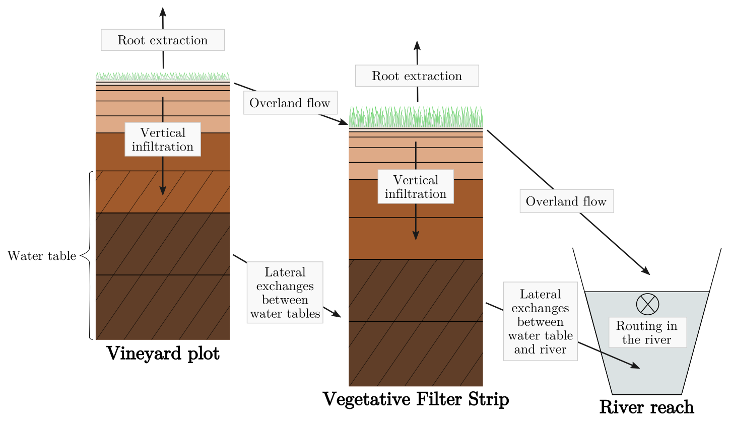
Figure 1 Discretization of landscape elements and physical processes included in the PESHMELBA version of this study. The horizontal black lines in the left and middle soil columns delimit the numerical cells, while the hatched areas represent the water tables. In these columns, the different brown fillings delimit the different soil horizons.

2.2 Data assimilation methods

The following sections introduce the ensemble Kalman filter, the ensemble smoother with multiple data assimilation, and the iterative ensemble Kalman smoother with multiple data assimilation. These methods aim to estimate the probability density function (PDF) of a state vector conditional on available observations. In this case study, we aim to estimate three-dimensional moisture profiles and some input parameters of the PESHMELBA model. The corresponding system state vector at time t_k with $k\in \mathit{\{}\mathrm{1},\mathrm{\dots },K\mathit{\}}$ is denoted x_k∈ℝⁿ in what follows. We assume available observations of mean moisture in the top 5 cm of the soil, and the corresponding observation vector at time t_k is denoted ${\mathit{y}}_k^{\mathrm{o}}\in {\mathbb{R}}^p$.

The model ${\mathcal{M}}_{k\to k+\mathrm{1}}:{\mathbb{R}}^n\to {\mathbb{R}}^n$ propagates the state vector from time t_k to time t_k+1 (Eq. 1), and ${\mathcal{H}}_k:{\mathbb{R}}^n\to {\mathbb{R}}^p$ is the observation operator that maps the state variable space onto the observation space at each time step (Eq. 2):

$$\begin{array}{}\text{(1)}& {\displaystyle }{\mathit{x}}_{k+\mathrm{1}}& {\displaystyle }={\mathcal{M}}_{k\to k+\mathrm{1}}\left({\mathit{x}}_k\right)+{\mathbf{v}}_k,\text{(2)}& {\displaystyle }{\mathit{y}}_k^{\mathrm{o}}& {\displaystyle }={\mathcal{H}}_k\left({\mathit{x}}_k\right)+{\mathbf{z}}_k,\end{array}$$

where v_k and z_k are the state error and the observation error respectively. They are assumed to be unbiased and to follow a Gaussian distribution:

$$\begin{array}{}\text{(3)}& {\displaystyle }{\mathbf{v}}_k\sim \mathcal{N}(\mathbf{0},{\mathbf{P}}_k),\text{(4)}& {\displaystyle }{\mathbf{z}}_k\sim \mathcal{N}(\mathbf{0},{\mathbf{R}}_k),\end{array}$$

where ${\mathbf{P}}_k\in {\mathbb{R}}^{n\times n}$ (resp. ${\mathbf{R}}_k\in {\mathbb{R}}^{p\times p}$) is the model error covariance matrix (resp. observation error covariance matrix).

In the case of joint estimation, the state vector x_k is augmented with the model parameters to be estimated, and the model ${\mathcal{M}}_{k\to k+\mathrm{1}}$ also includes an evolution law for the estimated parameters in addition to the state dynamical evolution. As soil characteristics are not expected to change over time at the scale of interest, we have chosen a persistence law to represent the (non-)evolution of the parameters.

The DA methods introduced in the next sections are sequential and consist of an alternation of a forecast step and an analysis step. During the forecast step, the model propagates a background state x_k−1 from t_k−1 to t_k, resulting in a forecast state vector ${\mathit{x}}_k^{\mathrm{f}}$. This prior state is updated during the analysis step based on the available measurements. The analysis results in a posterior state ${\mathit{x}}_k^{\mathrm{a}}$ at time t_k that becomes the background for the next forecast step between t_k and t_k+1. Accordingly, any given vector a or matrix A derived from the forecast step is denoted a^f or A^f in what follows, while it is denoted a^a or A^a if it is calculated at the analysis step. Although they aim to solve the same problem derived from the Bayes theorem, the methods tested in this study differ in the time window that is considered in the forecast step and the number of measurements simultaneously used in the analysis step. The distinct approximations and assumptions they are based on may lead to significantly different solutions that are analysed in this study. Their common structure and characteristics are summarized in Fig. 2.

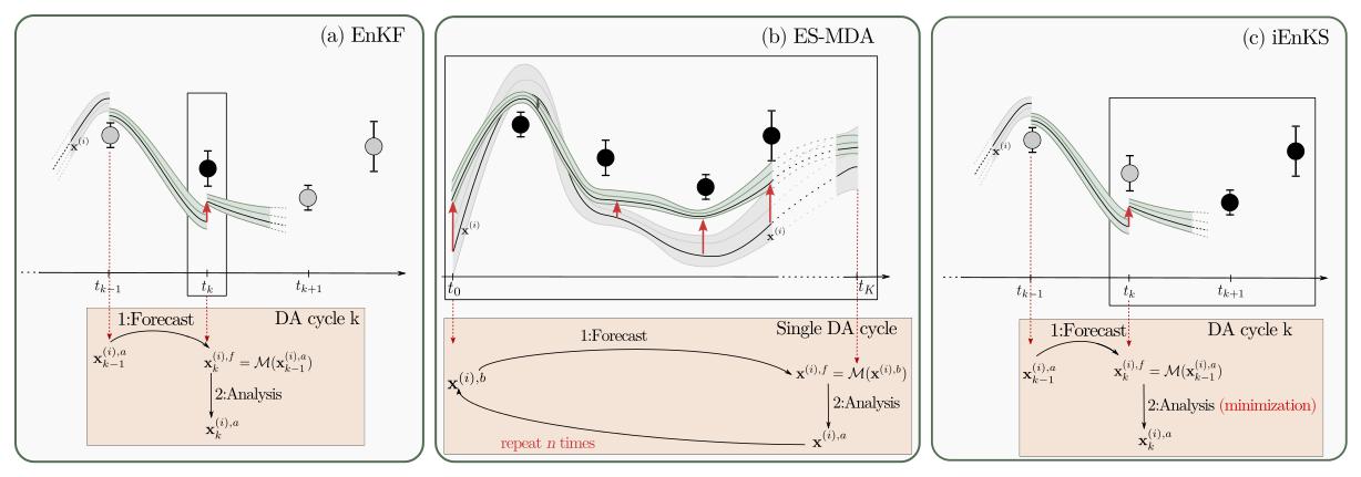
Figure 2 Schematic view of one DA cycle for the EnKF (a), the ES-MDA (b), and the iEnKS (c). The lines depict trajectories for some members of the ensemble, and the coloured envelop represents the ensemble uncertainty. The dots depict the available observations. The black dots in the black window are the observations that are used for the current DA cycle, whereas the grey dots are unused observations.

2.2.1 Ensemble Kalman filter

The ensemble Kalman filter (EnKF; Evensen, 1994) extends the Kalman filter resolution of the Bayesian estimation problem to nonlinear, high-dimensional contexts. The state distribution is approximated by an ensemble of M state vectors ${\mathit{x}}^{\left(i\right)},i\in \mathit{\{}\mathrm{1},\mathrm{\dots },M\mathit{\}}$. Each vector is sequentially propagated during the forecast step by applying the nonlinear model ℳ and updated during the analysis step using the current observations (see Fig. 2, left). This study is based on the ensemble transform Kalman filter (ETKF; Bishop et al., 2001; Hunt et al., 2007). At each time t_k, we consider ${\mathbf{X}}_k^{\mathrm{f}}\in {\mathbb{R}}^{n\times M}$, the matrix of normalized perturbations whose columns are expressed as

$$\begin{array}{}\text{(5)}& [{\mathbf{X}}_k^{\mathrm{f}}{]}_i={\displaystyle \frac{{\mathit{x}}_k^{\left(i\right),\mathrm{f}}-{\stackrel{\mathrm{‾}}{\mathit{x}}}_k^{\mathrm{f}}}{\sqrt{M-\mathrm{1}}}},\end{array}$$

with

$$\begin{array}{}\text{(6)}& {\stackrel{\mathrm{‾}}{\mathit{x}}}_k^{\mathrm{f}}={\displaystyle \frac{\mathrm{1}}{M}}\sum _{i=\mathrm{1}}^M{\mathit{x}}_k^{\left(i\right),\mathrm{f}}.\end{array}$$

During the analysis step, one looks for a state vector ${\mathit{x}}_k^{\mathrm{a}}$ in the affine subspace spanned by the anomalies: ${\stackrel{\mathrm{‾}}{\mathit{x}}}_k^{\mathrm{f}}+\mathrm{Vec}\mathit{\{}{\mathit{x}}_k^{\left(\mathrm{1}\right),\mathrm{f}}-{\stackrel{\mathrm{‾}}{\mathit{x}}}_k^{\mathrm{f}},\mathrm{\dots },{\mathit{x}}_k^{\left(M\right),\mathrm{f}}-{\stackrel{\mathrm{‾}}{\mathit{x}}}_k^{\mathrm{f}}\mathit{\}}$. The analysis is then expressed as

$$\begin{array}{}\text{(7)}& {\mathit{x}}_k^{\mathrm{a}}={\stackrel{\mathrm{‾}}{\mathit{x}}}_k^{\mathrm{f}}+{\mathbf{X}}_k^{\mathrm{f}}{\mathit{w}}_k,\end{array}$$

where w_k∈ℝ^M is a weight vector in the ensemble subspace. The optimal weight vector is obtained from the Kalman filter equation:

$$\begin{array}{}\text{(8)}& {\mathit{x}}_k^{\mathrm{a}}={\stackrel{\mathrm{‾}}{\mathit{x}}}_k^{\mathrm{f}}+{\mathbf{K}}_k[{\mathit{y}}_k^{\mathrm{o}}-{\mathcal{H}}_k({\stackrel{\mathrm{‾}}{\mathit{x}}}_k^{\mathrm{f}}\left)\right],\end{array}$$

where the Kalman gain ${\mathbf{K}}_k={\mathbf{P}}_k^{\mathrm{f}}{\mathbf{H}}_k^{\top }({\mathbf{H}}_k{\mathbf{P}}_k^{\mathrm{f}}{\mathbf{H}}_k^{\top }+{\mathbf{R}}_k{)}^{-\mathrm{1}}$ is computed with the forecast error covariance matrix expressed from the ensemble: ${\mathbf{P}}_k^{\mathrm{f}}={\mathbf{X}}_k^{\mathrm{f}}{\mathbf{X}}_k^{{\mathrm{f}}^{\top }}$. Identification of terms using the Sherman–Morrison–Woodbury formula allows us to express the optimal weight vector w_k in the ensemble subspace:

$$\begin{array}{}\text{(9)}& {\mathit{w}}_k=({\mathbf{I}}_M+{\mathbf{Y}}_k^{{\mathrm{f}}^{\top }}{\mathbf{R}}_k^{-\mathrm{1}}{\mathbf{Y}}_k^{\mathrm{f}}{)}^{-\mathrm{1}}{\mathbf{Y}}_k^{{\mathrm{f}}^{\top }}{\mathbf{R}}_k^{-\mathrm{1}}{\mathit{\delta }}_k,\end{array}$$

where δ is the innovation vector ${\mathit{\delta }}_k={\mathit{y}}_k^{\mathrm{o}}-{\mathcal{H}}_k\left({\stackrel{\mathrm{‾}}{\mathit{x}}}_k^{\mathrm{f}}\right)$ that contains the observations and where ${\mathbf{Y}}_k^{\mathrm{f}}\in {\mathbb{R}}^{p\times M}$ contains the observation normalized perturbations:

$$\begin{array}{}\text{(10)}& [{\mathbf{Y}}_k^{\mathrm{f}}{]}_i={\displaystyle \frac{{\mathcal{H}}_k\left({\mathit{x}}_k^{\left(i\right),\mathrm{f}}\right)-{\stackrel{\mathrm{‾}}{\mathit{y}}}_k^{\mathrm{f}}}{\sqrt{M-\mathrm{1}}}},\end{array}$$

with

$$\begin{array}{}\text{(11)}& {\stackrel{\mathrm{‾}}{\mathit{y}}}_k^{\mathrm{f}}={\displaystyle \frac{\mathrm{1}}{M}}\sum _{i=\mathrm{1}}^M{\mathcal{H}}_k\left({\mathit{x}}_k^{\left(i\right),\mathrm{f}}\right).\end{array}$$

The posterior ensemble of perturbations is generated so as to be representative of the posterior uncertainty that can be factorized as ${\mathbf{P}}_k^{\mathrm{a}}={\mathbf{X}}_k^{\mathrm{a}}{\mathbf{X}}_k^{{\mathrm{a}}^T}$. The analysis normalized anomalies are then derived:

$$\begin{array}{}\text{(12)}& {\mathbf{X}}_k^{\mathrm{a}}={\mathbf{X}}_k^{\mathrm{f}}({\mathbf{I}}_M+{\mathbf{Y}}_k^{{\mathrm{f}}^{\top }}{\mathbf{R}}^{-\mathrm{1}}{\mathbf{Y}}_k^{\mathrm{f}}{)}^{-\frac{\mathrm{1}}{\mathrm{2}}}.\end{array}$$

This leads to the following expression for the analysed members ${\mathit{x}}_k^{\left(i\right),\mathrm{a}},\forall i\in \mathit{\{}\mathrm{1},\mathrm{\dots },M\mathit{\}}$:

$$\begin{array}{}\text{(13)}& {\mathit{x}}_k^{\left(i\right),\mathrm{a}}={\stackrel{\mathrm{‾}}{\mathit{x}}}_k^{\mathrm{f}}+{\mathbf{X}}_k^{\mathrm{f}}({\mathit{w}}_k+\sqrt{M-\mathrm{1}}[({\mathbf{I}}_M+{\mathbf{Y}}_k^{{\mathrm{f}}^{\top }}{\mathbf{R}}^{-\mathrm{1}}{\mathbf{Y}}_k^{{\mathrm{f}}^{\top }}{)}^{\frac{-\mathrm{1}}{\mathrm{2}}}{]}_i).\end{array}$$

The ETKF is favoured for high-dimension problems as it alleviates the computational cost of the analysis. Indeed, most of the algebraic calculations are performed in the ensemble subspace, which is generally of a smaller dimension than the state or observation space.

2.2.2 Ensemble smoother with multiple data assimilation

The above section has introduced a filtering approach that is a sequential scheme based on incremental updates of the state vector x. For each update, the present system state PDF is corrected by Eq. (12) using present observations only. In contrast, the ensemble smoother (ES; van Leeuwen and Evensen, 1996) aims to estimate a posterior distribution for the state vector in an assimilation window $[t_{\mathrm{1}},\mathrm{\dots },t_K]$, relying on all observations available in that window. First, the ensemble is integrated over the whole assimilation window in a single forecast step. The augmented state vector x is composed of temporal trajectories for each state variable at each point of the model grid along with input parameters. The same analysis as for EnKF is then carried out, using all the observations at the same time (see Fig. 2, middle). The state variable trajectories are updated in space and time through space–time covariances estimated from the ensemble (Crestani et al., 2013).

More recently, Emerick and Reynolds (2013a) introduced the ensemble smoother with multiple data assimilation (ES-MDA), an “iterative version” that consists of iteratively performing the ES-like sequence: ensemble model integration over the whole assimilation window followed by an analysis step. It should be noted that the number of iterations is prescribed before launching the DA procedure and does not depend on a convergence criterion. At iteration (j), the analysis step from Eq. (12) is replaced by

$$\begin{array}{}\text{(14)}& {\mathbf{X}}_{\left(j\right)}^{\mathrm{a}}={\mathbf{X}}_{\left(j\right)}^{\mathrm{f}}({\mathbf{I}}_M+{\mathbf{Y}}^{{\mathrm{f}}^{\top }}{\mathit{\alpha }}_{\left(j\right)}^{-\mathrm{1}}{\mathbf{R}}^{-\mathrm{1}}{\mathbf{Y}}^{\mathrm{f}}{)}^{-\frac{\mathrm{1}}{\mathrm{2}}},\end{array}$$

where the notation ${\mathbf{X}}_k^{\mathrm{a}}$ (resp. ${\mathbf{X}}_k^{\mathrm{f}}$ and ${\mathbf{Y}}_k^{\mathrm{f}}$) for time t_k has been simplified to X^a (resp. X^f and Y^f) and where the weight α_(j) is an inflation term for the observation error covariance matrix R. Considering J, the predefined total number of iterations in the ES-MDA full scheme, the weights ${\mathit{\alpha }}_{\left(j\right)},j\in \mathit{\{}\mathrm{1},\mathrm{\dots },J\mathit{\}}$ must satisfy

$$\begin{array}{}\text{(15)}& \sum _{j=\mathrm{1}}^J{\displaystyle \frac{\mathrm{1}}{{\mathit{\alpha }}_{\left(j\right)}}}=\mathrm{1}.\end{array}$$

In this study, we set ${\mathit{\alpha }}_{\left(j\right)}=J,\forall j\in \mathit{\{}\mathrm{1},\mathrm{\dots },J\mathit{\}}$ (Emerick and Reynolds, 2013a; Cui et al., 2020).

The model integration at iteration (j+1) is then initialized with the posterior distribution of parameters obtained from the analysis at iteration (j). This scheme replaces a single abrupt analysis by several smaller analyses.

2.2.3 Iterative ensemble Kalman smoother with multiple data assimilation

As with the EnKF, the iEnKS alternates forecast and analysis steps to perform incremental updates of the state. However, in this fixed-lag smoothing context, each analysis aims to update a state vector at time t_k using observations between t_k+1 and t_k+L, where L is the length of the data assimilation window (DAW; see Fig. 2, right). Moreover, in contrast to the EnKF and the ES-MDA, the iEnKS fundamentally belongs to the category of variational methods. As such, the iEnKS analysis step consists of minimizing a cost function deduced from the Bayesian estimation problem formulation:

$$\begin{array}{}\text{(16)}& \begin{array}{rl}\mathcal{I}\left({\mathit{x}}_k^{\mathrm{a}}\right)& ={\displaystyle \frac{\mathrm{1}}{\mathrm{2}}}\parallel {\mathit{x}}_k^{\mathrm{a}}-{\mathit{x}}_k^{\mathrm{f}}{\parallel }_{{\mathbf{P}}_k^{\mathrm{f}}}^{\mathrm{2}}+\sum _{l=\mathrm{1}}^L{\displaystyle \frac{\mathrm{1}}{\mathrm{2}}}\parallel {\mathbf{y}}_{k+l}\\ & -{\mathcal{H}}_{k+l}\circ {\mathcal{M}}_{k\to k+l}\left({\mathit{x}}_k^{\mathrm{a}}\right){\parallel }_{{\mathbf{R}}_{k+l}}^{\mathrm{2}},\end{array}\end{array}$$

where $\parallel \mathit{x}{\parallel }_{\mathbf{A}}^{\mathrm{2}}={\mathit{x}}^{\top }\mathbf{A}\mathit{x}$. Like the EnKF and the ES, the iEnKS is an ensemble-based method, and the calculations rely on M members: ${\mathit{x}}^{\left(i\right)},i\in \mathit{\{}\mathrm{1},\mathrm{\dots },M\mathit{\}}$. X denotes the perturbation matrix (see Eq. 5).

At time t_k, the analysed state vector is expressed as an incremental correction ${\mathit{x}}_k^{\mathrm{a}}={\stackrel{\mathrm{‾}}{\mathit{x}}}_k^{\mathrm{f}}+{\mathbf{X}}_k^{\mathrm{f}}\mathit{w}$, and the minimization consists of finding the weight vector ${\mathit{w}}^{*}\in {\mathbb{R}}^M$ that minimizes the cost function expressed in the ensemble subspace. Again, the forecast error covariance matrix is expressed from the ensemble: ${\mathbf{P}}_k^{\mathrm{f}}={\mathbf{X}}_k^{\mathrm{f}}{\mathbf{X}}_k^{{\mathrm{f}}^{\top }}$, leading to the following expression for the cost function:

$$\begin{array}{}\text{(17)}& \begin{array}{rl}\mathcal{I}\left(\mathit{w}\right)& ={\displaystyle \frac{\mathrm{1}}{\mathrm{2}}}\parallel \mathit{w}{\parallel }^{\mathrm{2}}+\sum _{l=\mathrm{1}}^L{\displaystyle \frac{\mathrm{1}}{\mathrm{2}}}\parallel {\mathbf{y}}_{k+l}\\ & -{\mathcal{H}}_{k+l}\circ {\mathcal{M}}_{k\to k+l}({\stackrel{\mathrm{‾}}{\mathit{x}}}_k^{\mathrm{f}}+{\mathbf{X}}_k^{\mathrm{f}}\mathit{w}){\parallel }_{{\mathbf{R}}_{k+l}}^{\mathrm{2}},\end{array}\end{array}$$

where $\parallel \mathit{w}{\parallel }^{\mathrm{2}}={\mathit{w}}^{\mathrm{T}}\mathit{w}$.

The minimization of the cost function ℐ is performed in the ensemble subspace by a Gauss–Newton algorithm:

$$\begin{array}{}\text{(18)}& {\mathit{w}}_{(j+\mathrm{1})}={\mathit{w}}_{\left(j\right)}-{\mathbf{A}}_{\left(j\right)}^{-\mathrm{1}}\mathrm{\nabla }{\mathcal{I}}_{\left(j\right)}\left({\mathit{w}}_{\left(j\right)}\right),\end{array}$$

where (j) is the iteration index, A is an approximation of the Hessian of ℐ, and ∇ is the gradient operator. Such minimization actually corresponds to a nonlinear update.

The approximated Hessian and the gradient are expressed using the tangent linear of the operator transporting from the ensemble space to the observation space

$$\mathcal{H}\circ \mathcal{M}:{\mathbf{Y}}_{k+l,\left(j\right)}=[{\mathcal{H}}_{k+l}\circ {\mathcal{M}}_{k\to k+l}{]}_{|{\mathit{x}}_{k,\left(j\right)}}^{\prime }{\mathbf{X}}_k^{\mathrm{f}}.$$

In this study and as proposed in Bocquet and Sakov (2013), this tangent linear operator is estimated using finite differences (“bundle” iEnKS version). Both A and ∇ℐ are then computed from the ensemble:

$$\begin{array}{}\text{(19)}& {\displaystyle }{\mathit{x}}_{k,\left(j\right)}^{\mathrm{a}}={\stackrel{\mathrm{‾}}{\mathit{x}}}_k^{\mathrm{f}}+{\mathbf{X}}_k^{\mathrm{f}}{\mathit{w}}_{\left(j\right)},\text{(20)}& {\displaystyle }\begin{array}{rl}\mathrm{\nabla }{\mathcal{I}}_{\left(j\right)}& ={\mathit{w}}_{\left(j\right)}-\sum _{l=\mathrm{1}}^L{\mathit{\alpha }}_l{\mathbf{Y}}_{k+l,\left(j\right)}^T{\mathbf{R}}_{k+l}^{-\mathrm{1}}[{\mathbf{y}}_{k+l}\\ & -{\mathcal{H}}_{k+l}\circ {\mathcal{M}}_{k\to k+l}\left({\mathit{x}}_{k,\left(j\right)}^{\mathrm{a}}\right)],\end{array}\text{(21)}& {\displaystyle }{\mathbf{A}}_{\left(j\right)}={\mathbf{I}}_M+\sum _{l=\mathrm{1}}^L{\mathit{\alpha }}_l{\mathbf{Y}}_{k+l,\left(j\right)}^T{\mathbf{R}}_{k+l}^{-\mathrm{1}}{\mathbf{Y}}_{k+l,\left(j\right)},\end{array}$$

where ${\mathit{\alpha }}_l,l\in \mathit{\{}\mathrm{1},\mathrm{\dots },L\mathit{\}}$ values are inflation weights for the observation error. As the ensemble size is generally rather small, A_(j) can be inverted using direct exact methods. As with the ES-MDA, the iEnKS implementation chosen in this paper allows each observation to be used several times. The weights α_l then merely measure the impact of each observation in the DAW. The sum of the weights for an assimilation cycle respects

$$\begin{array}{}\text{(22)}& \sum _{l=\mathrm{1}}^L{\mathit{\alpha }}_l=\mathrm{1}.\end{array}$$

In Bocquet and Sakov (2014), a heuristic justification of this MDA scheme is given. The reader should refer to this paper for more details about this scheme. In this study, we choose a uniform scheme so that ${\mathit{\alpha }}_l=\frac{\mathrm{1}}{L},\forall l=\mathrm{1},..,L$.

The minimization takes place until a convergence criterion is reached. Then, the analysed members ${\mathit{x}}_k^{\left(i\right),\mathrm{a}},\forall i\in \mathit{\{}\mathrm{1},\mathrm{\dots },M\mathit{\}}$ are deduced at time t_k using the minimized vector w^* and the associated state vector ${\mathit{x}}_k^{\mathrm{a}}$:

$$\begin{array}{}\text{(23)}& {\mathit{x}}_k^{\left(i\right),\mathrm{a}}={\mathit{x}}_k^{\mathrm{a}}+\sqrt{M-\mathrm{1}}[{\mathbf{X}}_k^{\mathrm{f}}{\mathrm{H}}^{-\frac{\mathrm{1}}{\mathrm{2}}}{]}_i.\end{array}$$

This way, the iEnKS offers to perform the nonlinear update of the state as in standard variational DA (Carrassi et al., 2018).

2.3 Case study

In this study, we aim to investigate the accuracy and the robustness of the aforementioned DA methods in a simulation exercise based on PESHMELBA. To do so, we perform synthetic (or twin) DA experiments on a simplified, virtual catchment. DA experiments are conducted on the Morcille-like virtual catchment described in Rouzies et al. (2023). This size-limited catchment is inspired from the La Morcille catchment, situated in the Beaujolais vineyard region east of France. A comprehensive description of the setup can be found in their study, and its main characteristics are reported in what follows. The virtual catchment is composed of 10 vineyard plots, 4 VFSs, and a portion of river that delimits two hillslopes. All soil columns are 4 m deep. They are vertically discretized into 25 numerical cells whose thickness ranges from 0.05 m at the top to 1 m at the bottom. Three soil units (SUs), mainly sandy, compose the catchment, in accordance with the soil composition of the La Morcille catchment. Each soil type is made up of the vertical succession of three or four soil horizons. Each soil horizon is characterized by its own hydrodynamical behaviour that results in distinct sets of parameters. Figure 3 summarizes the scenario composition, the different SUs, and their vertical constitution. Vineyard plots and VFSs from the same SU are parameterized identically except for the first soil horizon. The first soil horizon is chosen to extend to the first 15 cm in VFSs, while it can vary on vineyard plots. Its main parameters are set in order to account for the effect of increased soil structuring and dense vegetation that mitigate surface runoff on VFSs. This way, the saturated hydraulic conductivity, the ponding height, and the roughness are increased compared with vineyard plots.

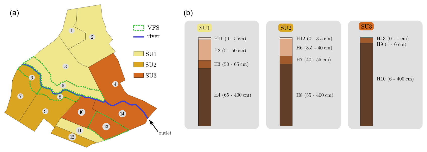
Figure 3 (a) Composition and spatial distribution of SUs in the virtual catchment. VFSs are bounded with the dashed green line, while the remaining mesh units are vineyard plots. (b) Details of SU constitution in terms of succession of soil horizons on vineyard plots. SU constitutions for VFSs are the same except for the surface horizon that is 15 cm deep.

Vineyard plot and VFS pressure profiles are initialized considering hydrostatic equilibrium and initial water table levels that are consistent with field data for the given time period. Realistic rain and potential evapotranspiration forcings that correspond to a typical winter period in the area are used. Except for atmospheric forcings, all boundary conditions are zero fluxes. Two vegetation types are set in this scenario. A vineyard cover is considered on plots, while a permanent, mature grassland is parameterized on VFSs. Root depth and root density are supposed to be constant all over the simulation for both of them, while the leaf area index (LAI) evolves over the simulation period for vineyard cover. LAI remains constant on grassland.

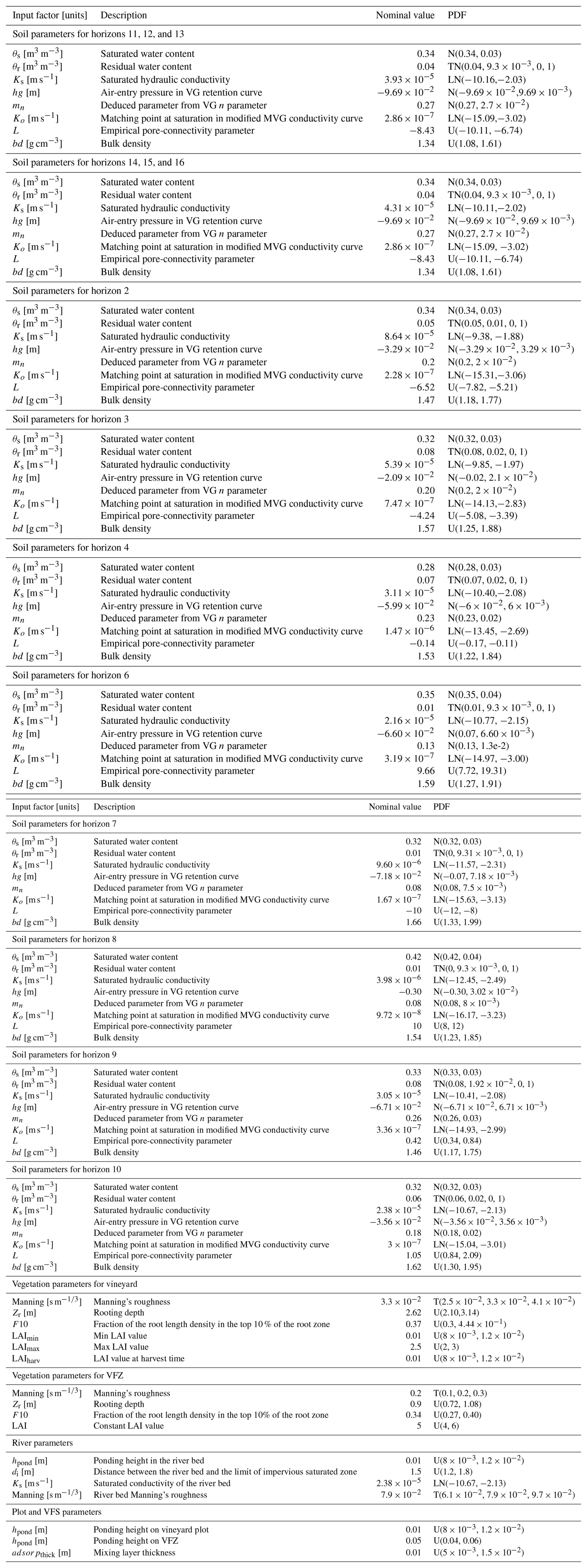
The full scenario results in 128 parameters whose nominal values and meaning are described in Appendix A. Some input parameters may seem redundant from one soil horizon to another, but we explicitly distinguish between several horizons in order to prepare setups that include pesticide transfers. In such an application, parameters will need to vary from one horizon to the other.

As a reference for result interpretation, Fig. 4 shows an example of nominal time series of moisture at different depths (surface, intermediate, and deep). At the surface, soil moisture dynamics are strongly driven by rain forcings all over the simulation. In contrast, moisture varies significantly only after 1200 h of simulation at 0.2 m depth, when stronger rain events occur. Finally, at 4 m depth, the system is not affected by the dynamics from superficial cells or climate forcings. It remains in a steady state that corresponds to the presence of a water table, leading to a constant moisture value.

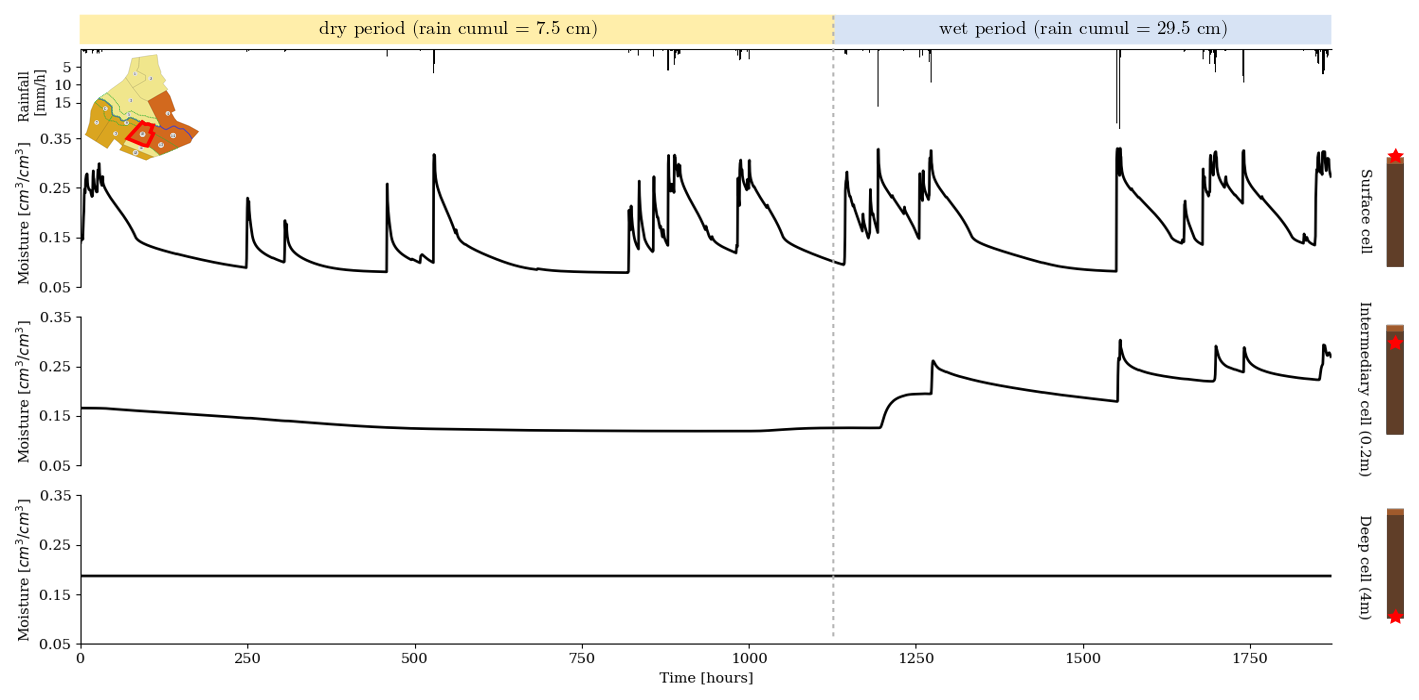
Figure 4 Soil moisture time series for the nominal simulation on plot 10 at the surface (top), 0.2 m depth (middle), and 4 m depth (bottom). Rain forcings are shown in the top black histogram, while the position of plot 10 in the catchment is denoted by a red line in the top-left pictogram. The soil composition of plot 10 is shown in the soil columns depicted on the right, with red stars showing the corresponding depths.

2.4 DA setup

As this study focuses on twin experiments, we use synthetic images that mimic satellite moisture data in the top 5 cm. Such data are supposed to come from the synergistic use of optical and radar signals from Sentinel-1 and Sentinel-2 satellites (Bousbih et al., 2018), which in turn can be converted into maps of surface soil moisture in agricultural areas (El Hajj et al., 2017; Gao et al., 2017). The synthetic images are generated from a “true” reference run of PESHMELBA and are perturbed with Gaussian, non-biased noise. Observation errors are supposed to be uncorrelated in time and space, and the standard deviation for error is set to 0.02 cm³ cm⁻³ at the first step. It should be noted that this approximate for observation error is underestimated compared with values found in Bousbih et al. (2018). In this paper, the authors conducted experiments on cereal crops. To our knowledge, similar experiments on vineyards have not been performed yet. Observation error for such soil cover may differ greatly, and sensitivity to the observation error magnitude is thus investigated in this study. We assume a time series is available for mean moisture in the top 5 cm for each vineyard plot and VFS in the catchment. The observation operator ℋ is accordingly built as a matrix so as to relate each observation to the weighted mean of moisture over the six numerical cells that compose the top 5 cm of the soil column:

$$\begin{array}{}\text{(24)}& {\mathit{\theta }}_{\mathrm{5}\mathrm{cm}}={\displaystyle \frac{{\sum }_{j=\mathrm{1}}^{\mathrm{6}}{\mathit{\theta }}_j\mathrm{d}{z}_j}{{\sum }_{j=\mathrm{1}}^{\mathrm{6}}\mathrm{d}{z}_j}},\end{array}$$

where θ_j and dz_j are the soil moisture and the thickness of numerical cell j respectively.

For the sake of simplicity, we consider that the input parameters are the only sources of uncertainty in the model. The ensemble is initialized by independently perturbing the 128 input parameters. Perturbations are set according to each input parameter PDF. Such a PDF has been defined from field measurements, the literature, and expert knowledge in a previous study (Rouzies et al., 2023). They are detailed in Appendix A.

Joint estimation is performed in order to estimate both vertical moisture profiles and relevant uncertain input parameters. The global sensitivity analysis of PESHMELBA in this case study showed that parameters that influence moisture profiles the most are mainly θ_s (water contents at saturation) for the different soil horizons (Radišić et al., 2023). The augmented state vector thus includes these 14 parameters for both surface and deeper soil horizons, and a bias is added to their PDFs when generating the initial ensemble.

For the iEnKS, the number of Gauss–Newton iterations in the cost function minimization is set to three, which, from experience, can limit the cost and is considered enough (Eq. 18 being solved exactly). A preliminary sensitivity study also allowed us to set the iEnKS optimal DAW length L so as to assimilate observations by a batch of five. Similarly, from preliminary trials, the number of iterations is set to three for the ES-MDA.

The nominal scenario consists of a 78 d simulation with 6 d observation frequency, a standard deviation for observation error equal to 0.02 cm³ cm⁻³, and an ensemble size of 50 members. Then, a series of experiments is set up in order to assess the robustness of the DA methods and to test their sensitivity to the (1) observation error magnitude, (2) observation frequency, and (3) ensemble size. To do so, each factor (observation error magnitude, observation frequency, and ensemble size) is varied individually, while the others are set up to nominal values. Tested values are reported in Table 1.

Table 1 Scenarios explored to assess the sensitivity of DA methods to the (i) observation error (standard deviation), (ii) frequency of observation, and (iii) ensemble size. Nominal values are in bold.

The performances of the DA methods in the different setups are assessed by computing the continuous ranked probability score (CRPS; Brown, 1974) on the moisture time series, on each vineyard plot, and the VFS at the surface and at 0.2 and 4 m depths. The CRPS expresses the distance between the cumulative density function (CDF) of the probabilistic forecast and the CDF of a reference. In this case, the reference is the “true” run of PESHMELBA that is supposed to be free of error. Its CDF is built using the Heaviside function, and the CRPS consists of building the quadratic distance between the two functions:

$$\begin{array}{}\text{(25)}& \text{CRPS}(\mathrm{Y},\widehat{\mathit{\theta }})=\underset{-\mathrm{\infty }}{\overset{\mathrm{\infty }}{\int }}\left[F_Y\right(s)-H(s-\widehat{\mathit{\theta }}){]}^{\mathrm{2}}\mathrm{d}s,\end{array}$$

where F_Y is the CDF of the one-dimensional ensemble of moisture values Y, $\widehat{\mathit{\theta }}$ is the deterministic value of moisture from the PESHMELBA “true” run, and H(x) is the Heaviside function. It is a positive error criterion variable: the closer it is to 0, the better is the ensemble forecast. The CRPS is expressed in the same unit as the evaluated variable. It is averaged over time/space in the case of a multidimensional forecast Y. In this study, CRPS scores are estimated following Hersbach (2000), and the corresponding formulation is detailed in Appendix B. In order to better capture the impact of DA on the simulation, we also use the continuous ranked probability skill score (CRPSS), which is the ratio between the CRPS of the analysis and the CRPS of the free run (i.e. the unassimilated state):

$$\begin{array}{}\text{(26)}& \text{CRPSS}=\mathrm{1}-{\displaystyle \frac{{\mathrm{CRPS}}_{\mathrm{DA}}}{{\mathrm{CRPS}}_{\mathrm{free}}}},\end{array}$$

where CRPS_DA (resp. CRPS_free) is the CRPS score of the analysis (resp. the free run). When positive, the closer the CRPSS is to 1, the more the DA process improves the estimation. When negative, the assimilation process degrades the estimation compared with the free run.

As pointed out in Bocquet and Sakov (2014), it is crucial to remind the reader that the performances of a DA scheme depend on the metrics chosen to assess its quality. We chose the CRPS because it rigorously generalizes the notion of mean absolute error (MAE) to stochastic predictions. In addition, the decomposition of the average CRPS can also provide information on the reliability and the resolution of the posterior ensemble (Hersbach, 2000).

3 Results

3.1 Comparison of methods

3.1.1 Performances on moisture variable correction

The three DA methods are first tested on the nominal setup presented in Sect. 2.4. Figure 5 compares the CRPS time series of moisture variables assimilated by the three DA methods with the free run simulation on plot 10. The evolution of the CRPS for both the free run and the assimilated state is highly correlated to the precipitation time series. Rainfall events and the following recession periods lead to peaks in the CRPS chronicle, showing an increased level of uncertainty in the system in wet conditions. During the first three assimilation cycles (up to 576 h), the iEnKS and the EnKF decrease the error to a limited extent compared with the free run. More precisely, in this first part of the simulation, the corrections from their analysis steps have nearly no effect after each rainfall event that follows an analysis. Until 576 h, the ES-MDA is then the only method that allows for a clear reduction in the CRPS, during both rainfall events and dry periods. The second part of the simulation is characterized by longer and more intense rainfall events. In this time period, all methods allow for an effective decrease in the model error. Broadly speaking, the ES-MDA leads to lower CRPS values and smaller discrepancies between dry and wet periods, showing comparable performances for both hydrological regimes.

Figure 5 Comparison of CRPS time series for the free run and the different DA methods on plot 10's surface compartment. The position of plot 10 is depicted by the red line in the top-right map, while the position of the surface cell in the associated soil column is depicted by the red star. The rainfall chronicle is shown in the top histogram, while vertical grey lines correspond to times when surface moisture observations are available.

Unlike surface moisture estimation, the three methods exhibit much more limited performances in the subsurface, as shown in Fig. 6. At 0.2 m depth, the soil only reacts to stronger rain events from 1200 h, once again leading to peaks in the CRPS series within this time period. Again, the ES-MDA performs the best in decreasing the error, although the gain from the free run is much more limited than for surface estimation. The iEnKS generally degrades the moisture estimation, especially between 1000 and 1250 h. The iEnKS is the only method that is characterized by moving DA windows. During each analysis, the current state is corrected using the next L observations (L=5 in this case). The change in the model dynamics between the analysis time step and the following observation time steps observed in the intermediary cell after 1200 h (see Fig. 4, middle) may explain such poor correction of the state by the iEnKS.

In the deeper cell, the CRPS remains constant between each analysis step (see Fig. 4, bottom). The EnKF and the ES-MDA also achieve a limited decrease in CRPS compared with the free run, whereas the iEnKS once again degrades the estimation. Note that from 1152 h, the iEnKS no longer performs analysis because there are not enough observations available in the DAW. The system is no longer corrected from this moment onwards.

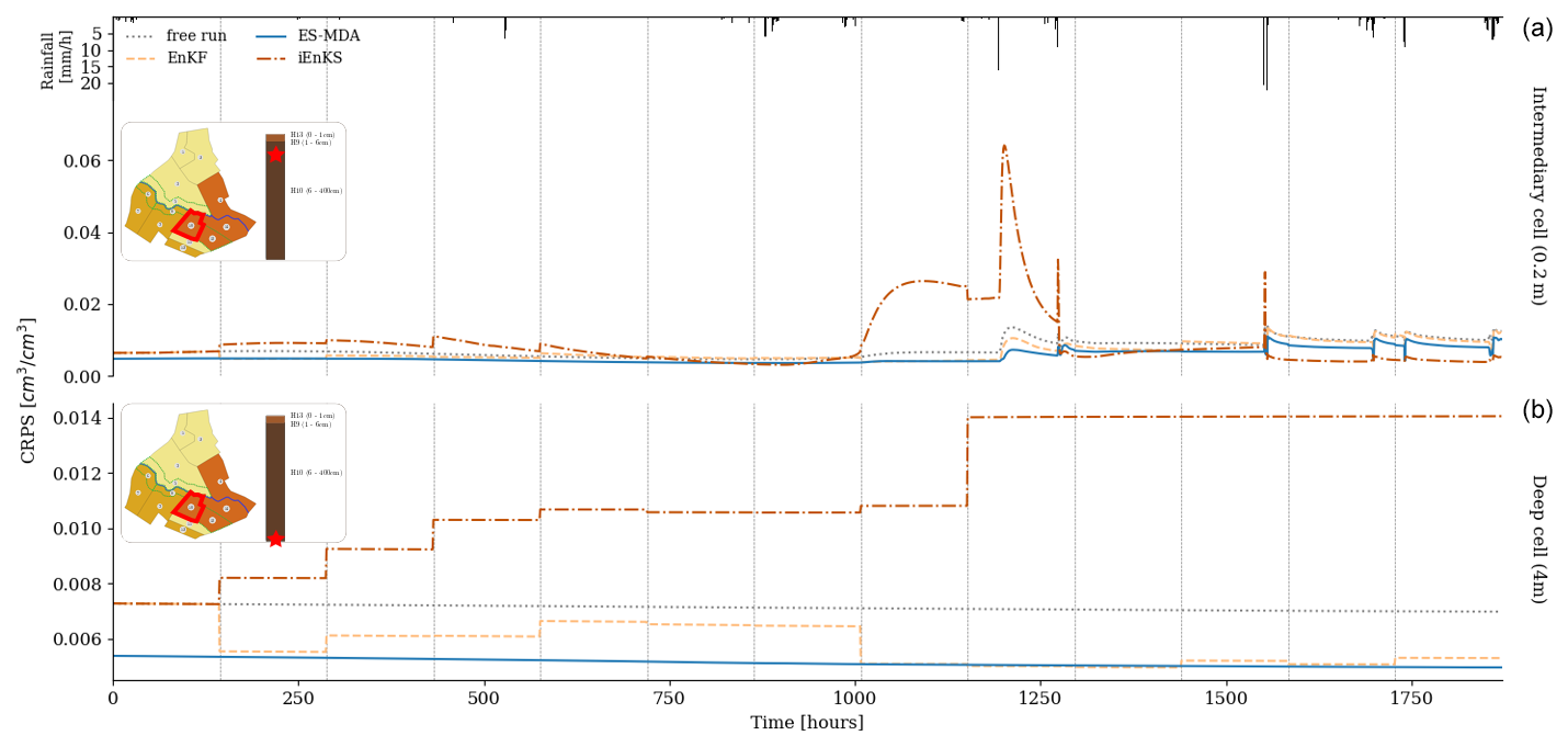
Figure 6 Comparison of CRPS time series for the free run and the different DA methods in the intermediary cell (0.2 m depth, a) and the deeper cell (4 m depth, b) for plot 10. The position of plot 10 is depicted by the red line in the top-right map, while the position of the cell in the associated soil column is depicted by the red star. The rainfall chronicle is shown in the top histogram, while vertical grey lines correspond to time steps when surface moisture observations are available.

The average CRPSSs over the whole temporal period and the whole catchment at the scrutinized depths are computed for the three methods in order to quantitatively identify the most appropriate DA method for the PESHMELBA model. All methods significantly improve moisture estimation at the surface, with CRPSSs being superior, with an average value of 0.38. The ES-MDA almost always outperforms the EnKF and the iEnKS at the surface and, to a lesser extent, at the subsurface (Fig. 7). Conversely, the EnKF significantly degrades the state estimate in the middle cells for most of the HUs (Hydrological Units) (negative CRPSS value). In the deeper cell, the ES-MDA also outperforms the EnKF on average (0.15 vs. 0.06), while the iEnKS leads to significantly increased error compared to the free run. However, when looking locally, better CRPSSs are performed by the ES-MDA on 9 out of the 14 UHs, which makes it impossible to generalize. Indeed, the contribution of assimilation is much more limited in the intermediary compartment, which is not observed and not significant in the deep compartment.

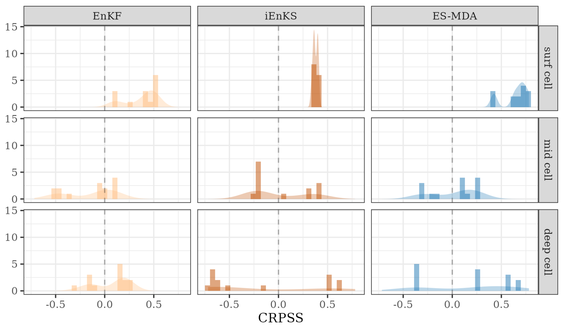
Figure 7 Distribution over the 14 HUs (Hydrological Units) of CRPSS averaged over time. The vertical line at a CRPSS of 0 highlights a decrease in error compared with the free run (positive values) or an increase in error compared to the free run (negative values).

3.1.2 Performances on parameter estimation

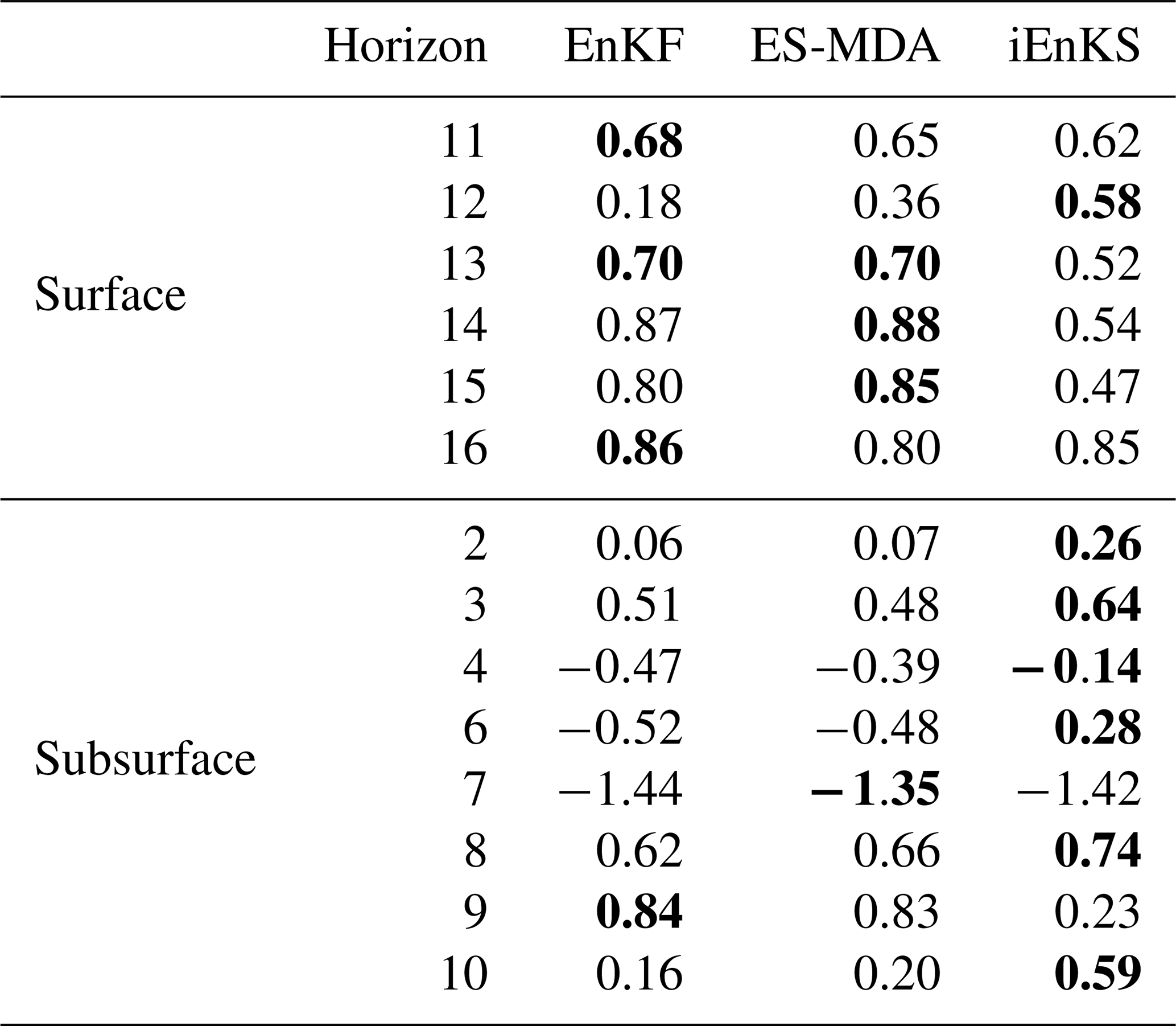
Performances on parameter estimation are also assessed, and Fig. 8 shows the posterior PDFs of the estimated water contents at saturation θ_s, while Table 2 summarizes the associated CRPSS values. Estimation of θ_s for surface horizons is significantly improved by the three methods as CRPSS values exceed 0.58 in all cases. Still based on CRPSS values, the EnKF and the ES-MDA perform the best. Results are less clear-cut for the estimation of subsurface parameters. Indeed, CRPSS values are far lower than for the surface, and the DA process even degrades θ_s estimation for horizons 4, 7, and 6, except for the iEnKS. For subsurface parameters, the iEnKS tends to perform the best, although it once again achieves limited performances compared with surface parameter estimation. While the EnKF and the ES-MDA rely on the correlation matrix to estimate unobserved parameters, the iEnKS builds a cost function that explicitly relates to the input parameters. The full correlation matrix (not shown here) shows that there is little to no correlation between the moisture in the upper 5 cm and the parameters in the subsurface, which may explain why the iEnKS performs better in such compartments. Finally, for both surface and subsurface parameters, the posterior PDF and the associated CRPSS values obtained from the EnKF and the ES-MDA are quite close. It shows that assimilating observations one by one or all at once, using an ensemble-Kalman-filter-based method, leads to comparable performances for parameter estimation, whereas significant differences are noticed for variable correction.

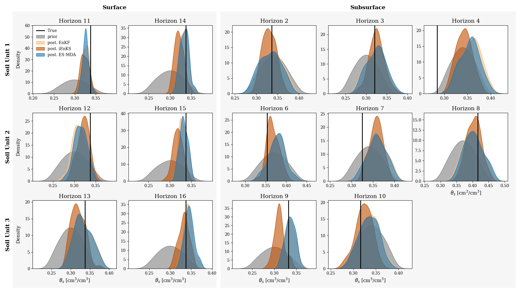
Figure 8 Empirical PDFs for estimated surface parameters for SU1 (top line), SU2 (middle line), and SU3 (bottom line). The first column shows PDFs of surface θ_s on vineyard plots, while the second column refers to surface parameters on VFSs. The remaining columns represent parameters for subsurface horizons. The true values of the parameters are indicated by the vertical black line in each plot.

Table 2 CRPSS values associated with parameter estimation for the three DA methods. Positive values indicate a decrease in error compared with the free run, while negative values indicate an increase in error compared with the free run. For each line, the bold value refers to the best estimate.

3.1.3 Computational cost

The computational costs of the three methods are differ considerably. The EnKF is the fastest method (277 CPU hours), followed by the ES-MDA (558 CPU hours) and the iEnKS (2143 CPU hours). Compared with the EnKF, both the ES-MDA and the iEnKS perform incremental corrections, leading to higher computational costs. Furthermore, in the case of the iEnKS, using an assimilation window of size L implies that the model must be integrated up to $M\times L\times jmax$ times to perform each analysis. As PESHMELBA integration is the most costly step in the assimilation process, the iEnKS computational cost ends up being much more significant than for the other methods.

3.2 Sensitivity of the methods to DA setup

In this section, the sensitivity of the different methods to observation error prescription, assimilation frequency, and ensemble size is investigated. As the tested DA methods have shown limited performance in retrieving subsurface moisture from satellite surface moisture images, the analysis focuses on surface moisture estimation, following several scenarios (Table 1). Furthermore, as mentioned in the previous section, the high computational cost of the iEnKS is prohibitive for performing intensive exploration of the method in this case study. Sensitivity analysis is then only performed for the two methods with the highest potential in this application, EnKF and ES-MDA.

3.2.1 Observation error

The sensitivity to the observation error magnitude is tested on a setup with a frequency of assimilation of 6 d (144 h) and an ensemble size of 50 on a 78 d long simulation and evaluated on averaged CRPSS (Fig. 9). As expected, for both methods, the CRPSS is the highest for small observation errors and regularly decreases for larger observation errors. In the case of the EnKF, no significant correction of the state can be obtained from error values higher than 0.1 cm³ cm⁻³. In the case of the ES-MDA, moisture is noticeably corrected for error values up to 0.2 cm³ cm⁻³.

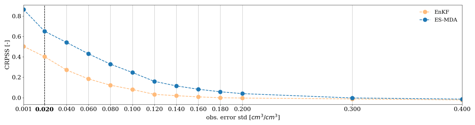
Figure 9 CRPSS sensitivity to the standard deviation of the observation error for the surface cell with the EnKF and ES-MDA. The CRPSS is computed as an average over the whole time series and over the whole catchment. The bold label and vertical dashed line denote the nominal value of the observation error used in this case study.

3.2.2 Frequency of observation

The averaged CRPSS in the surface compartment for the EnKF and the ES-MDA is also evaluated as a function of the observation frequency (Fig. 10). The observation error magnitude is set to 0.02 cm³ cm⁻³, and the ensemble size is set to 50. In the case of the EnKF, the CRPSS is relatively stable for observation frequencies (meaning analysis frequencies) up to 72 h and decreases regularly for lower frequencies. ES-MDA performances are rather stable for frequencies of observation less than 144 h (6 d). Performances are slightly worse for frequencies of 192 and 216 h (even if they are still higher than the best-performing EnKF setup) and drop significantly if observations are available only every 240 h (10 d).

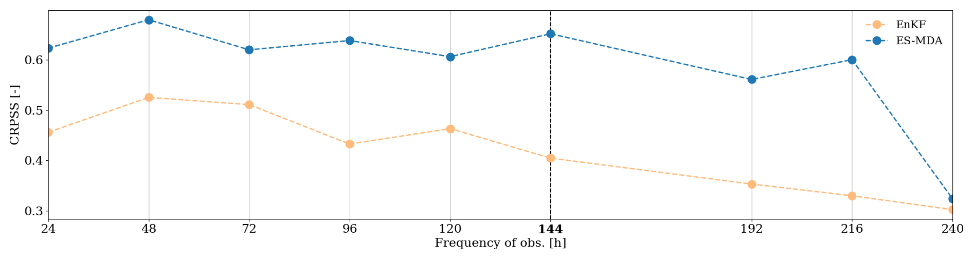
Figure 10 Comparison of the CRPSS sensitivity to observation frequency for the surface cell. The CRPSS is computed as an average over the whole time series and over the whole catchment. The bold label and vertical dashed line denote the nominal frequency of the observation. This value also corresponds to a realistic frequency of observation for surface moisture images used in this case study.

3.2.3 Ensemble size

While the observation error magnitude and the observation frequency are intrinsic properties of the observation set in practice, the ensemble size is a parameter of the DA setup that can be tuned by the user. Its choice also critically impacts the numerical cost of the data assimilation and should be chosen to reach a satisfying trade-off between limited computational cost and sufficient accuracy of the analysis. In this experiment, the sensitivity to the ensemble size is tested on a scenario with an observation error of 0.02 cm³ cm⁻³ and with a frequency of observations of 144 h (Fig. 11).

For both methods, the lower CRPSS value is reached for an ensemble size of 20. The EnKF performances stabilize for an ensemble size higher than 50 members, while 100 members are necessary for the ES-MDA, partly due to its higher state vector size that includes a temporal dimension.

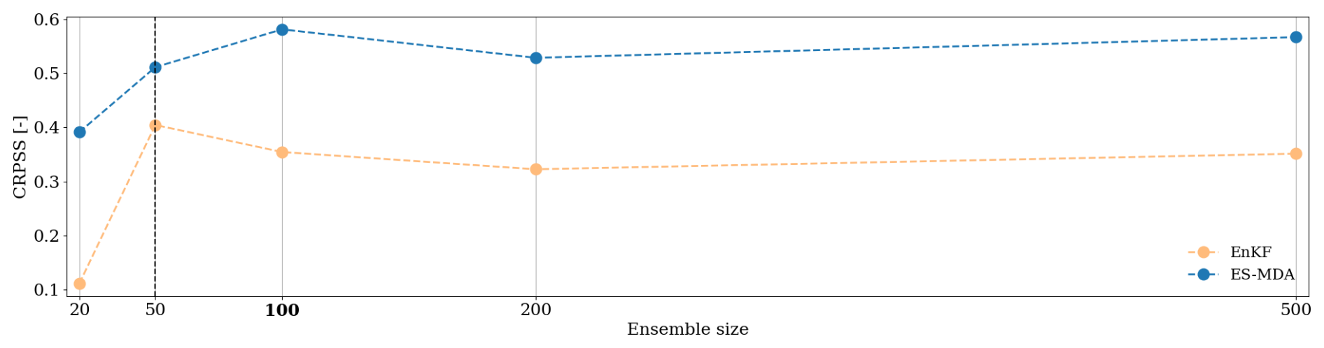
Figure 11 CRPSS sensitivity to the ensemble size for the surface cell. The CRPSS is computed as an average over the whole time series and over the whole catchment. The bold label and vertical dashed line denote the nominal value of the ensemble size used in this case study.

4 Discussion

4.1 On the choice of the DA method

Results from the above section indicate that in this case study, assimilating observations one at a time is sufficient for estimating input parameters. However, integrating several observations simultaneously is more efficient for correcting moisture trajectories, particularly when using the ensemble smoother with multiple data assimilation. The ES-MDA better constrains the system as it incorporates information from all observations and the system dynamics, making it especially effective in coping with nonlinearity, as noted by Emerick and Reynolds (2013a). The ES-MDA ensures that corrections can propagate from observed to unobserved times, particularly from rainy periods to inter-event periods, given sufficient temporal correlations. In contrast, during the initial dry hydrological regime, saturated water contents (θ_s) are unobservable, limiting the performances of the EnKF and the iEnKS, which correct the augmented state vector at a specific time. The global and iterative correction of the ES-MDA allows the impact of accurate observations during wet periods to extend to unobservable dry periods. In addition, although the iEnKS demonstrates potential for parameter estimation, it is clear that the additional computational cost for moisture correction is not worth it. This is likely because the PESHMELBA modular approach results in the linear coupling of the one-dimensional vertical Richards equation through lateral Darcy's law, rather than employing the nonlinear full three-dimensional Richards equation. Such linear coupling reduces the potential benefits of using iEnKS on highly nonlinear systems.

From the above, the ES-MDA is identified as the best compromise for assimilating moisture images for the joint estimation of moisture profiles and θ_s parameters in the PESHMELBA model. The ES-MDA performs the best for moisture correction and achieves performances comparable to those of the EnKF for parameter estimation. This method is also straightforward to implement and does not require frequent interruptions of the calculation code to perform the analysis. Additionally, although the ES-MDA is an iterative method, its computational cost remains reasonable, as only a few iterations are necessary to optimize its performances.

4.2 On the real-case DA implementation

The exploration of DA implementation scenarios (Sect. 3.2) allows us to suggest some practical guidelines to best adapt the setup to the PESHMELBA model. First, the quality of assimilated data plays a crucial role: the results provide users of moisture data obtained from Sentinel-1/Sentinel-2 synergistic inversion with guidelines on the required quality of future observations over vineyard cover. For example, one could keep in mind that an error in observations less than 0.05 cm³ cm⁻³ with the EnKF (resp. 0.1 cm³ cm⁻³ with the ES-MDA) will be required to reach significant improvements (higher than 20 % compared with the free run) in surface moisture estimation. Regarding the frequency of data, it is set to 144 h on average for surface moisture images computed from the Sentinel-1 and Sentinel-2 satellites. In this application, this frequency is nearly optimal, all other factors being equal, for maximizing the performances of the ES-MDA for DA window lengths of around 3 months, as all observations are integrated at the same time. In the case of the EnKF, a frequency of 72 h would be necessary to optimize its performances.

Finally, an ensemble size of 100 members is advised for both methods to ensure a stable performance, as this size is often chosen in studies that describe their DA experiment setup in hydrology (Camporese et al., 2009; Nie et al., 2011; Lei et al., 2020).

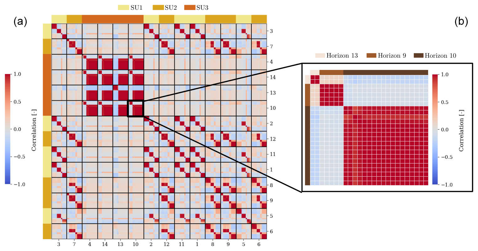
Figure 12 (a) Correlation matrix of the ensemble after 144 h of simulation in the free run. Vertical and horizontal lines delimit the numerical cells from the same plot. The top and left colours indicate the soil type for each plot, while the bottom and right indices are the plot indices. (b) Portion of the correlation matrix that relates to plot 10. Each square outlined in white refers to a numerical cell in the vertical profile of plot 10. The top and left colours refer to the soil horizon for each numerical cell.

4.3 On the limitations of the methods

Even if the different DA methods succeed in estimating surface variables and parameters, the gain is limited to retrieving subsurface variables and parameters. Moisture observations only cover the top 5 cm, and none of the tested methods properly retrieve deeper values. In theory, both the iEnKS and the ES-MDA, which are characterized by longer DAW lengths, may have been able to capture the subsurface dynamics if they had remained correlated to the surface dynamics. However, the correlation matrices extracted at some time steps, such as those shown in Fig. 12, and for the whole time series (not shown here) show that there are nearly no correlations between the surface and the subsurface, even when considering potential time lags. In this case study, the composition of each soil type with distinct horizons, as well as the vertical discretization, which is much more refined at the surface than at the subsurface, may explain the lack of correlation. It should be noted that such a lack of correlation has also been observed in Bonan et al. (2020) (in arid contexts only).

We conclude that assimilating observations of topsoil moisture cannot properly correct subsurface variables or parameters. However, from the correlation matrix (Fig. 12), we see that the moisture in a given soil horizon is highly correlated to the moisture in this same soil horizon in other plots that also contain this specific soil horizon. This means that observations of a full soil column in some points in the catchment may be sufficient to correct all plots with the same soil type. This option must be further investigated, for example, by assimilating measurements from electronic magnetic interference that can provide punctual pseudo-observations of soil moisture vertical profiles. In this case, we would need to introduce a new observation error model since the moisture profiles would be deduced from resistivity measurements. Figure 12 also highlights the absence of spatial correlations between soil units of different soils, advocating the use of a scheme with a local domain DA in the ES-MDA (Asch et al., 2016) to alleviate the computational cost of this method that uses high-dimension matrices.

5 Conclusions

In this study, we set a rigorous data assimilation framework for a modular model that is specifically built for water quality management. The conducted experiments were aimed not only at retrieving vertical moisture profiles but also at estimating certain input parameters, based on synthetic surface moisture satellite images. To do so, we implemented several stochastic ensemble methods, namely the ensemble Kalman filter, the ensemble smoother with multiple data assimilation, and the iterative ensemble Kalman smoother. These three methods are representative of the spectrum of available ensemble methods (ensemble filters, hybrid ensemble/variational smoothers, and long-window ensemble smoothers). They solve the DA problem differently, and, in particular, they use the available observations in different ways. We then assessed and compared their performances for joint estimation so as to choose the most appropriate method for the PESHMELBA model.

Results of the comparison showed that all methods performed well in retrieving moisture and parameters at the surface, but the ES-MDA significantly outperformed the EnKF and the iEnKS. The ES-MDA is indeed the only method that can fully integrate the system dynamics in its analysis step. Results for the subsurface, however, showed that all methods failed in retrieving the rest of the vertical moisture profiles and associated saturated water content parameters. The analysis of the correlation matrices showed that the surface and the subsurface compartments are poorly correlated, meaning that one should not expect surface moisture data alone to improve moisture estimates in deeper compartments. Furthermore, the results of analyses on the sensitivity to observation error, observation frequency, and ensemble size provided practical guidelines to implement an adapted DA setup in future operational applications.

As the proposed setup has been shown to be limited in retrieving subsurface moisture, further research could extend this study to multi-source data assimilation. For instance, the joint assimilation of surface moisture images and punctual observations of vertical moisture profiles obtained from electronic magnetic interference should be further investigated to improve moisture estimation in deep soil compartments. In addition, when setting up any stochastic DA experiment, the ensemble must be generated so as to represent the model error as accurately as possible. In this study, only the parameter values were considered a source of uncertainty, which is certainly too simplistic. Future experiments should then integrate uncertainty in initial conditions and climate forcings.

Systematically taking into account and reducing the uncertainties in risk assessment models is a major issue, especially when these models have an operational impact. This study paves the way for further applications in risk assessment models, even based on a complex structure, to assess both water and pollutant transfers in agricultural landscapes.

Appendix A

Table A1 Input parameter description, nominal values, and PDFs.

Appendix B: Evaluation of the CRPS

Assuming an ensemble of M moisture values Y₁,…,Y_M sorted from the smallest to the largest so that

$$\begin{array}{}\text{(B1)}& Y_i\le Y_j,\text{ for }i<j,\end{array}$$

and so that $\widehat{\mathit{\theta }}$ is the deterministic reference value, the CRPS for the ensemble is evaluated as follows (Hersbach, 2000):

$$\begin{array}{}\text{(B2)}& \text{CRPS}=\sum _{i=\mathrm{0}}^M{\mathit{\alpha }}_i{p}_i^{\mathrm{2}}+{\mathit{\beta }}_i(\mathrm{1}-p_i{)}^{\mathrm{2}},\end{array}$$

where $p_i=\frac{\mathrm{1}}{M}$, and α_i and β_i are defined as follows:

$$\begin{array}{}\text{(B3)}& \begin{array}{ccc}\mathrm{0}<i<M& {\mathit{\alpha }}_i& {\mathit{\beta }}_i\\ & & \\ \widehat{\mathit{\theta }}>Y_i& Y_{i+\mathrm{1}}-Y_i& \mathrm{0}\\ Y_{i+\mathrm{1}}>\widehat{\mathit{\theta }}>Y_i& \widehat{\mathit{\theta }}-Y_i& Y_{i+\mathrm{1}}-\widehat{\mathit{\theta }}\\ \widehat{\mathit{\theta }}<Y_i& \mathrm{0}& Y_{i+\mathrm{1}}-Y_i\end{array}.\end{array}$$

The cases where i=0 and i=M only apply to the CRPS when the reference value $\widehat{\mathit{\theta }}$ is an outlier, meaning it is less than Y₁ or more than Y_M. In this case, Table B3 must be modified with the following:

$$\begin{array}{}\text{(B4)}& \begin{array}{ccc}\text{Outlier}& {\mathit{\alpha }}_i& {\mathit{\beta }}_i\\ & & \\ \widehat{\mathit{\theta }}<Y_{\mathrm{1}}& \mathrm{0}& Y_{\mathrm{1}}-\widehat{\mathit{\theta }}\\ Y_M<\widehat{\mathit{\theta }}& \widehat{\mathit{\theta }}-Y_M& \mathrm{0}\end{array}.\end{array}$$