Ensembling differentiable process-based and data-driven models with diverse meteorological forcing datasets to advance streamflow simulation

Streamflow simulations produced by different hydrological models exhibit distinct characteristics and can provide valuable information when ensembled. However, few studies have focused on ensembling simulations from models with significant structural differences and evaluating them under both temporal and spatial tests. Here we systematically evaluated and utilized the simulations from two highly different models with great performances: a purely data-driven long short-term memory (LSTM) network and a physics-informed machine learning (“differentiable”) HBV (Hydrologiska Byråns Vattenbalansavdelning) model (δHBV). To effectively display the features of the two models, multiple forcing datasets are employed. The results show that the simulations of LSTM and δHBV have distinct features and complement each other well, leading to better Nash-Sutcliffe model efficiency coefficients (NSE) and improved high-flow and low-flow metrics across all spatiotemporal tests, compared to within-class ensembles. Ensembling models trained on a single forcing outperformed a single model using fused forcings, challenging the paradigm of feeding all available data into a single data-driven model. Most notably, δHBV significantly enhanced spatial interpolation when incorporated into LSTM, and provided even more prominent benefits for spatial extrapolation where the LSTM-only ensembles degraded significantly, attesting to the value of the structural constraints in δHBV. These advances set new benchmark records on the well-known CAMELS (Catchment Attributes and Meteorology for Large-sample Studies) hydrological dataset, reaching median NSE values of ∼ 0.83 for the temporal test (densely trained scenario), ∼ 0.79 for the ungauged basin test (PUB, Prediction in Ungauged Basins), and ∼ 0.70 for the ungauged region test (PUR, Prediction in Ungauged Regions). This study advances our understanding of how various model types, each with distinct mechanisms, can be effectively leveraged alongside multi-source datasets across diverse scenarios.

1 Introduction

Streamflow, a critical component of the global hydrosphere, profoundly influences both human society and natural ecosystems (Lins and Slack, 1999). Accurate simulation and prediction of streamflow yield numerous benefits, including improved flood prevention strategies (Brunner et al., 2021). Hydrological models serve as indispensable tools for achieving this objective and can be traditionally categorized into two types: data-driven models (Feng et al., 2020; Kratzert et al., 2018; Liu et al., 2024; Nearing et al., 2024) and process-based (or physically-based) models (Newman et al., 2017; Paul et al., 2021). Data-driven models, exemplified by long short-term memory (LSTM) (Feng et al., 2020; Kratzert et al., 2018) and transformer (Liu et al., 2024) networks, excel in learning patterns from multi-source data (Li et al., 2023b, 2024; Liu et al., 2022; Nearing et al., 2024) and generally achieve high performance. However, they often lack interpretability and may not resolve extreme values very well (Li et al., 2020a; Song et al., 2025b). Conversely, process-based models, derived deductively from physical laws or conceptualized views of natural systems, offer insights into internal hydrological processes but may exhibit weaker performance due to structural inadequacies (Li et al., 2020a, 2022; Zhang et al., 2019).

To combine the benefits and counteract the weaknesses of these two kinds of models, many efforts have been made to incorporate physical constraints and structures into data-driven models to align with fundamental physical principles, such as mass and water balances (Bandai and Ghezzehei, 2021; Wang et al., 2020; Xie et al., 2021). The most seamless integration uses neural networks to provide parameterizations or missing process representations for process-based models (Aboelyazeed et al., 2023; Bindas et al., 2024; Feng et al., 2022; Jiang et al., 2020; Kraft et al., 2022; Rahmani et al., 2023; Song et al., 2024; Tsai et al., 2021). These differentiable models (Shen et al., 2023) connect (flexible amounts of) prior physical knowledge to neural networks, and have displayed many advantages, including improved computational efficiency and prediction of untrained variables (Tsai et al., 2021), spatial generalization (Feng et al., 2023b), and representation of extremes (Song et al., 2025b). However, it is also unclear whether current differentiable models, e.g., δHBV, the Hydrologiska Byråns Vattenbalansavdelning (HBV) model implemented within a differentiable framework (Feng et al., 2023b; Ji et al., 2025; Shen et al., 2023; Song et al., 2025b), have unique bias characteristics that are associated with the process-based parts of their structures that cannot be reduced once the equations are prescribed.

Orthogonal to such efforts are ensemble simulations (Yu et al., 2024), which combine many members with different biases and uncertainties to mitigate their respective biases in deterministic predictions. Many previous studies have tried ensemble methods to improve streamflow (Clark et al., 2016; Zounemat-Kermani et al., 2021) based on many factors, like initial conditions (e.g., initial weights and biases in LSTM; Kratzert et al., 2018), data used for parameterization (Feng et al., 2021), and objective functions (Lin et al., 2024). These studies generally use one model to generate the differences among the ensemble members. Furthermore, some studies (Dion et al., 2021; Solanki et al., 2025) have utilized simulations from multiple different models but are limited to process-based models, resulting in ensemble simulations that are better than each individual member. Thus far, however, most studies have focused on simulations from only similar models or model types, and little work has tested an ensemble across the boundary of model types, particularly between data-driven, process-based, and hybrid models, especially on a large number of samples. Presumably, if each model has its own unique bias, data-driven and process-based models are likely to exhibit greater differences due to their inherently distinct characteristics. It remains unclear whether ensembling across model types should bring benefits to deterministic predictions. Furthermore, grounded in the process-based model, the differentiable process-based hydrological model, such as δHBV, significantly enhances performance compared to traditional process-based models, while on the other hand introducing greater uncertainty regarding its potential benefits when ensembled. Moreover, previous studies have primarily focused on evaluating ensemble simulations for temporal predictions. However, streamflow simulation under spatial extrapolation scenarios presents greater challenges, and findings from temporal tests may not be directly applicable in this context.

It is known that the performance of any type of hydrologic model heavily depends on the quality of input data, particularly meteorological forcing data (Bell and Moore, 2000; Yao et al., 2020), and other inputs, like the uncertainties of initial conditions, can be mitigated via warming up (Yu et al., 2019). While independent forcing datasets excel in certain aspects, they each carry different error characteristics (Beck et al., 2017; Behnke et al., 2016; Newman et al., 2019) and accordingly affect the hydrological models in different ways. In order to fully display the different features between LSTM and δHBV, multiple forcing datasets could be considered. Given the utilization of multiple forcing datasets, one could choose to use data fusion to combine them into a single coherent model input (Kratzert et al., 2021; Sawadekar et al., 2025), or to pass each forcing dataset through a model and then afterwards combine the multiple outputs in an ensemble. It is not clear which approach is more beneficial.

Considering the knowledge gaps discussed above, we sought to answer several research questions:

1. Will a cross-model-type ensemble of LSTM and δHBV improve deterministic streamflow prediction more than a within-class ensemble?

2. Is it better to use multiple forcings in one model or to ensemble multiple models, each with a different forcing input?

3. Do process-based equations bring unique value to an ensemble, especially in terms of spatial generalizability?

The remainder of this paper is structured as follows: Sect. 2 outlines the hydrological data and models used in this study, as well as the experimental design. Results and discussions are presented in Sect. 3, with conclusions provided in Sect. 4.

2 Materials and methods

2.1 CAMELS hydrologic dataset

The Catchment Attributes and Meteorology for Large-sample Studies (CAMELS) dataset (Addor et al., 2017) is widely employed for hydrological model evaluation and community benchmarking. The CAMELS dataset encompasses 671 basins distributed across the conterminous United States, with basin sizes ranging from 1 to 25 800 km² (median: 335 km²). This standardized and publicly available dataset serves as a benchmark for evaluating various hydrological models, with LSTM models trained on this dataset often serving as a reference point for comparing other models (Kratzert et al., 2021). CAMELS provides basin-scale data, including streamflow observations and static basin attributes, as well as forcing datasets from three independent sources: Daymet (Thornton et al., 1997), North American Land Data Assimilation System (NLDAS) (Xia et al., 2012), and Maurer (Maurer et al., 2002). Each of the three meteorological forcing datasets operates at a daily temporal resolution, encompassing precipitation, temperature, vapor pressure, and surface radiation variables, with daily temperature extrema of NLDAS and Maurer supplemented from Kratzert et al. (2021). These three meteorological forcing datasets have methodological distinctions in spatial resolution, data generation approaches, and temporal processing (Behnke et al., 2016; Kratzert et al., 2021). Exemplary plots illustrating the differences among the three meteorological forcing datasets are provided in Appendix B. These features can lead to dataset-specific error characteristics and make them valuable for displaying the distinct features of different model types. All model inputs used in this study are detailed in Table C1 in Appendix C.

2.2 Long short-term memory

As one kind of deep learning algorithm, long short-term memory (LSTM) (Hochreiter and Schmidhuber, 1997) has unique structures like hidden states and gates activated by the tanh and sigmoid functions (Li et al., 2023a), respectively. These features enable LSTM to excel in streamflow simulation tasks (Feng et al., 2020; Kratzert et al., 2018; Nearing et al., 2024). In the current benchmark framework, LSTM models are trained using dynamic atmospheric forcings and static basin attributes as inputs, with streamflow as the target output, making it perform well in both temporal and spatial tests (Fig. 1a). In this work, for cross-group comparability, we used the LSTM model and its hyperparameters as reported in Kratzert et al. (2021).

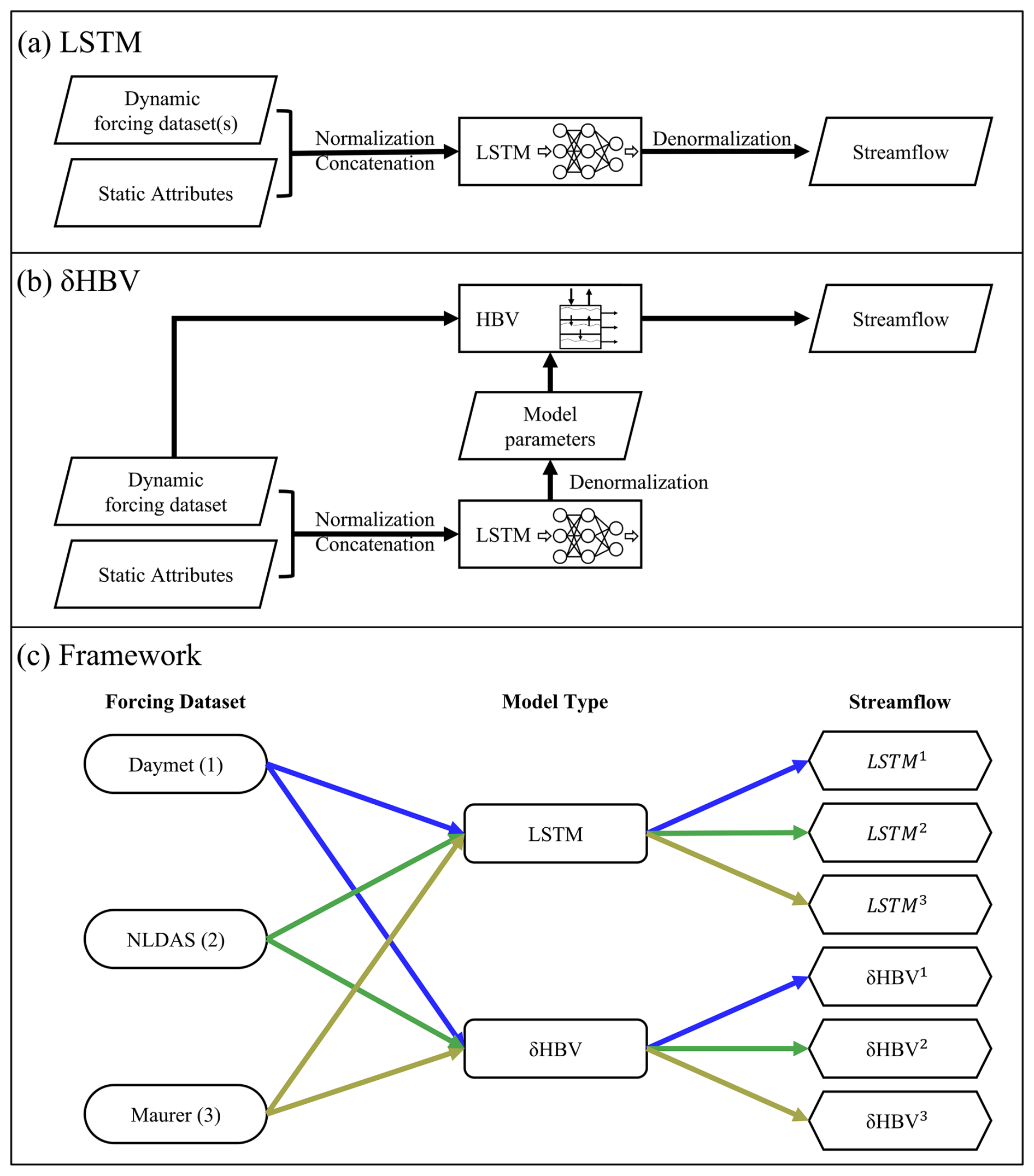
Figure 1 (a) The LSTM structure, (b) the δHBV structure, and (c) the framework to generate the six individual ensemble members of the streamflow simulations, in which different colors of arrow lines denote the different meteorological forcing datasets (also denoted as 1, 2, 3), respectively.

2.3 Differentiable HBV model (δHBV)

The Hydrologiska Byråns Vattenbalansavdelning (HBV) model is a parsimonious bucket-type hydrologic model that simulates various hydrological variables, including snow water equivalent, soil water, groundwater storage, evapotranspiration, quick flow, baseflow, and total streamflow (Aghakouchak and Habib, 2010; Beck et al., 2020; Bergström, 1976, 1992). Recently demonstrated differentiable HBV (δHBV) model (Feng et al., 2023b; Ji et al., 2025; Shen et al., 2023; Song et al., 2024) incorporates deep neural networks for both regionalized parameterization and missing process representations within a differentiable programming framework that supports “end-to-end” training (Fig. 1b). This innovation enables δHBV to effectively learn from data while obeying physical laws, resulting in high-level performance for streamflow simulations. From the perspective of process-based modeling, LSTM is a regionalized parameter provider that leverages the autocorrelated nature of its inputs to impose an implicit spatial constraint on the generated parameters.

In this study, we used δHBV1.1p (Song et al., 2024, 2025b), which is an updated version of δHBV1.0 (Feng et al., 2022, 2023b). The main improvement is the addition of a capillary rise module, which enhances the characterization of low flows. Three additional modifications are included to address high-flow simulation challenges: the use of three dynamic parameters (γ, β, k₀) (Song et al., 2025b); the removal of log-transform normalization for precipitation; and the adoption of the normalized squared-error loss function (Table C2) (Frame et al., 2022; Kratzert et al., 2021; Song et al., 2025a, b; Wilbrand et al., 2023). We also maintain dynamic parameters during warm-up periods. Although this provides only marginal benefits and increases computational costs, it yields a more realistic representation and reduces uncertainties associated with initial conditions. The basic equations in δHBV are as follows:

$$\begin{array}{}\text{(1)}& {\displaystyle }\mathit{\theta }={\mathrm{LSTM}}_{\mathrm{w}}(\stackrel{\mathrm{‾}}{x},\stackrel{\mathrm{‾}}{A_{\mathrm{attr}}})\text{(2)}& {\displaystyle }Q=\mathrm{HBV}(x,\mathit{\theta })\text{(3)}& {\displaystyle }{W}_{\mathrm{opt}}={\mathrm{argmin}}_{\mathrm{w}}\left(L\right(Q,Q^{\ast }\left)\right)\end{array}$$

where θ are the dynamic or static physical parameters, w denotes the weights and biases of LSTM, x includes the basin-averaged meteorological forcings, such as precipitation, mean temperature, and potential evapotranspiration, with $\stackrel{\mathrm{‾}}{x}$ representing their normalized versions. Similarly, $\stackrel{\mathrm{‾}}{A_{\mathrm{attr}}}$ consists of normalized observable basin-averaged attributes, encompassing basin area, topography, climate, soil texture, land cover, and geology (Table C1). Precipitation and mean temperature are from CAMELS, while potential evapotranspiration is calculated using the Hargreaves (1994) method based on maximum and minimum temperatures along with basin latitudes, all from data described in Sect. 2.1. Q and Q^∗ are the streamflow simulations (model outputs) and observations (as provided in CAMELS), respectively. HBV is implemented on PyTorch so it is programmatically differentiable: all steps store information related to gradient calculations during backpropagation, allowing this model to be trained together with neural networks in an end-to-end fashion. More details about differentiable HBV can be found in previous studies (Feng et al., 2022; Song et al., 2024). The details of some particularly relevant HBV processes are described in Appendix A.

2.4 Experimental design

In this study, we trained the two models of very different types (LSTM and δHBV), each with one of three meteorological forcing datasets (Daymet, NLDAS, and Maurer), resulting in six corresponding streamflow simulations (Fig. 1c) for each different test scenario (see Sect. 2.5 for additional information). The training processes of LSTM and δHBV followed Kratzert et al. (2021) and Feng et al. (2023b), respectively. Test results and performance metrics for all models are reported for the 531-basin subset that excludes those with areas larger than 2000 km² or with more than a 10 % discrepancy between different basin area calculation methods (Newman et al., 2017).

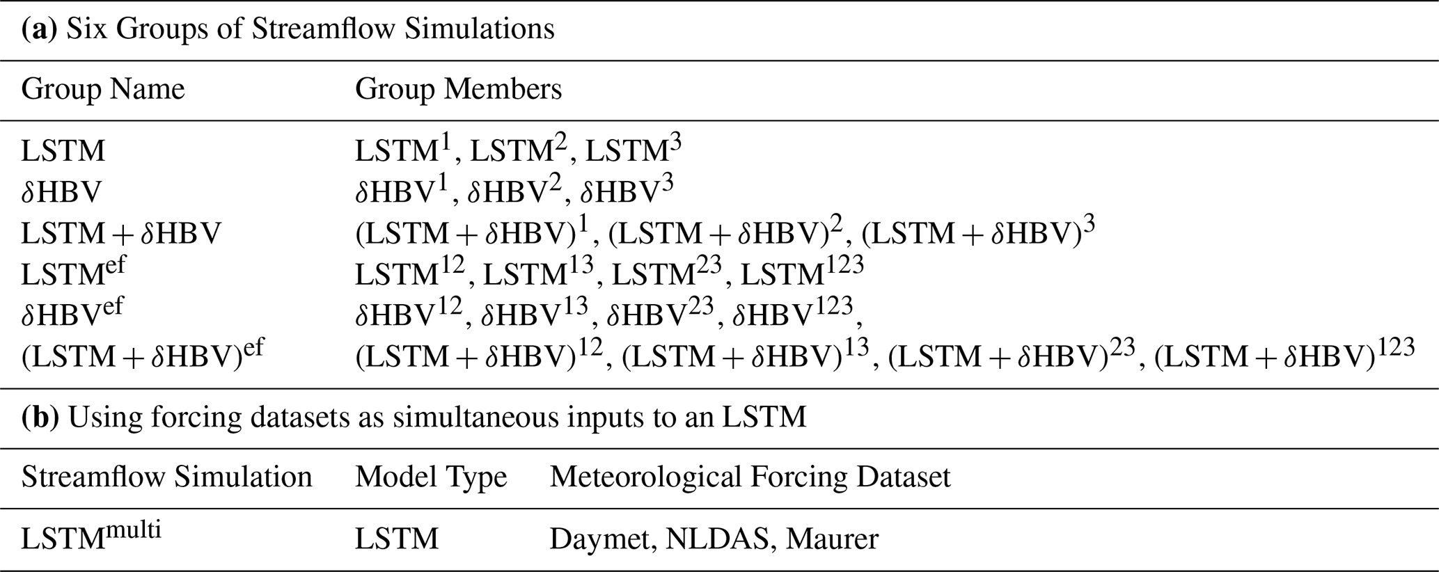
To generate ensembles, we tested various weighting strategies and ultimately employed averaging to combine the six single-forcing, single-model-type simulations, as it yielded the best performance. To better describe various combinations including cross-model ensembles, these simulations were categorized into six groups (Table 1). A shorthand notation is used throughout the remainder of this work to describe the forcing datasets and ensembles. Daymet, NLDAS, and Maurer are abbreviated as superscripts 1, 2, and 3, respectively. The + symbol is used to group model types being ensembled, while superscript clustering (e.g., ¹² or ¹²³) is used to group the meteorological forcing types being ensembled, with parentheses indicating that the superscripts apply to all model types within. For example, (LSTM+δHBV)¹²³ could be explicitly written as ${\mathrm{LSTM}}^{\mathrm{1}}+{\mathrm{LSTM}}^{\mathrm{2}}+{\mathrm{LSTM}}^{\mathrm{3}}+\mathit{\delta }{\mathrm{HBV}}^{\mathrm{1}}+\mathit{\delta }{\mathrm{HBV}}^{\mathrm{2}}+\mathit{\delta }{\mathrm{HBV}}^{\mathrm{3}}$. To compare two different strategies to utilize the multiple meteorological forcing datasets and to benchmark against the previously highest performance, we additionally trained a single LSTM model using all three forcing datasets as simultaneous inputs as done by Kratzert et al. (2021), referred to as LSTM^multi (the last row in Table 1).

Table 1 (a) The six groups of streamflow simulations, and (b) the streamflow simulation via LSTM based on a different strategy, in which three meteorological forcing datasets were combined as a single set of inputs (Kratzert et al., 2021). Superscripts 1, 2, and 3 denote Daymet, NLDAS, and Maurer, respectively. The ensemble across forcings (“ef”) superscript indicates an ensemble of model simulations, each of which uses a different single meteorological forcing, e.g., LSTM¹² means the average of LSTM¹ and LSTM².

2.5 Evaluation scenarios and criteria

The above cases were comprehensively evaluated for performance in temporal extrapolation (Feng et al., 2022; Kratzert et al., 2018), as well as two types of spatial generalization: prediction in ungauged basins (PUB) (Feng et al., 2023b; Kratzert et al., 2019), and prediction in ungauged regions (PUR) (Feng et al., 2021, 2023b):

• Temporal Test: Models were trained using data from all basins and tested across different periods.

• PUB Test: Models were trained on randomly selected subsets from all basins and tested on the remaining basins during the same time period.

• PUR Test: Different from the PUB test, basins were grouped into continuous regions, one of which was selected to comprise the group of testing basins while the others were used for training.

Temporal generalization is generally considered to be the easiest of these tests. In terms of spatial generalization, which approximates data-sparse scenarios, the PUB test is an example of spatial interpolation, whereas the PUR test involves spatial extrapolation. The PUR test is widely regarded as the most challenging and may therefore produce findings that differ significantly from those in other scenarios. In this study, all basins were divided into 10 spatially stratified groups for the PUB test and 7 fully disjoint regional groups for the PUR test (Table 2) in the same way as Feng et al. (2023b). The spatial extent of the 7 regions for the PUR test is also shown in Fig. 3c1–c2. Therefore, we conducted 10 rounds for the PUB test and 7 rounds for the PUR test, with a different group held out for testing in each round. Model performance was evaluated after concatenating the test results for all basins.

Table 2 Differences of temporal, PUB, and PUR tests.

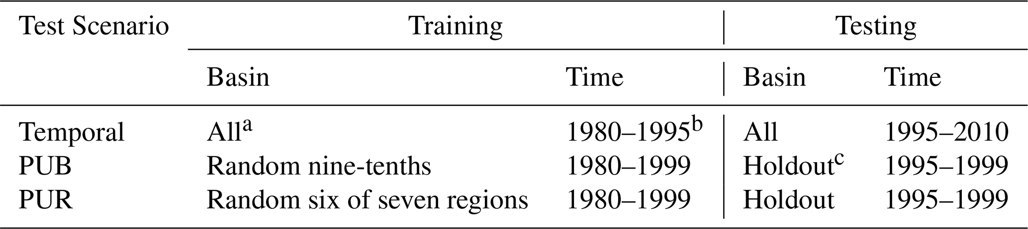
^a δHBV training followed Feng et al. (2023b) using all 671 CAMELS basins, while LSTM training followed Kratzert et al. (2021) using the selected 531-basin subset. Test results and performance metrics for all models are reported for the 531 basins. ^b Each hydrological year spans from 1 October to 30 September of the following year. ^c In the PUB and PUR tests, models are run for 10 and 7 rounds, respectively, with the group held out for testing changed in each round. The simulation performance was evaluated after concatenating the test results for all basins.

We repeated all the simulations with three different random seeds. Therefore, all the simulations come from a total of $(\mathrm{2}\times \mathrm{3}+\mathrm{1})\times (\mathrm{1}+\mathrm{10}+\mathrm{7})\times \mathrm{3}$ trained models. The first factor represents the models: two model types (LSTM and δHBV) trained separately with each of the three forcing datasets, along with LSTM^multi, a single model instance trained using all three forcing datasets simultaneously. The second factor accounts for the three types of tests (temporal, PUB, and PUR tests), and the last for the three random seeds. With respect to random seeds, we present two variations in the results, which are visually depicted in Fig. C1 in Appendix C. The results without “seed” as a subscript represent the average metric values from multiple streamflow simulations, each generated from a single model implementation, along with the corresponding uncertainties, visualized using error bars. The results marked with “seed” as a subscript are based on the average of multiple streamflow simulations conducted with different random seeds. In terms of computational cost, training LSTM (30 epochs) and δHBV (50 epochs) for temporal testing under a single meteorological forcing dataset takes approximately 5 and 21 h, respectively, using a single NVIDIA Tesla V100 GPU.

We calculated several well-established performance metrics: Nash-Sutcliffe model efficiency coefficient (NSE) (Nash and Sutcliffe, 1970), Kling-Gupta model efficiency coefficient (KGE) (Kling et al., 2012), percent bias (PBIAS), and root-mean-square error (RMSE). We also considered RMSE values for high (top 2 % “peak” flow, highRMSE), low (bottom 30 % “low” flow, lowRMSE), and mid-range (the remaining flow, midRMSE) flow conditions (Yilmaz et al., 2008). These metrics were computed for each basin and aggregated into error bars and cumulative density functions (CDFs). For brevity, the main text primarily reports NSE values, and other metric values are provided in Appendices D and E. Furthermore, we use the spread values (Li et al., 2021; Reichle and Koster, 2003) to investigate ensemble variability and explore model complementarity. Detailed descriptions of these metrics and their calculations are available in Table C2.

3 Results and discussion

3.1 Temporal extrapolation

For the temporal test, in which models were trained and tested on the same basins but in different time periods, we found that cross-model-type ensembles noticeably surpassed the within-class ensembles when other conditions were the same, with small uncertainties as shown by the error bars in Fig. 2. With a single forcing dataset, the median NSE was elevated from ∼ 0.735 for LSTM to ∼ 0.79 with δHBV added, though δHBV performance was similar to LSTM (∼ 0.74 under Daymet). Even after LSTM achieved very high performance when its simulations, each derived separately from different meteorological forcing datasets, were ensembled (ef = 123, ∼ 0.808), adding δHBV still improved the results to ∼ 0.818. This finding was robust for all different combinations of the tested meteorological forcing datasets. Conversely, adding LSTM also helped to improve δHBV ensembles. These results highlight the benefits of the cross-model-type ensemble framework and indicate distinct simulation features for each model type. LSTM is a data-driven method that has low bias and large variance. Data errors (Li et al., 2020b), different sampling strategies (Nai et al., 2024), or even different weight initializations (Narkhede et al., 2022) can lead to substantively different outcomes. Conversely, δHBV may have a smaller variance but a larger bias due to the fixed HBV formulation (Moges et al., 2016) for some scenarios like low flows (Feng et al., 2023b; Song et al., 2024) or in basins with significant water uses (Song et al., 2025a). These errors with varying characteristics from different model classes can partially offset each other in an ensemble. On a side note, δHBV models seem more reliant on the quality of the forcing data, as shown in Fig. 2. δHBV with the Maurer and NLDAS forcing datasets generally performs worse than it does with Daymet, which has lower biases. However, even in those cases, the combination of LSTM and δHBV was still better than LSTM alone, attesting to the robustness of these benefits.

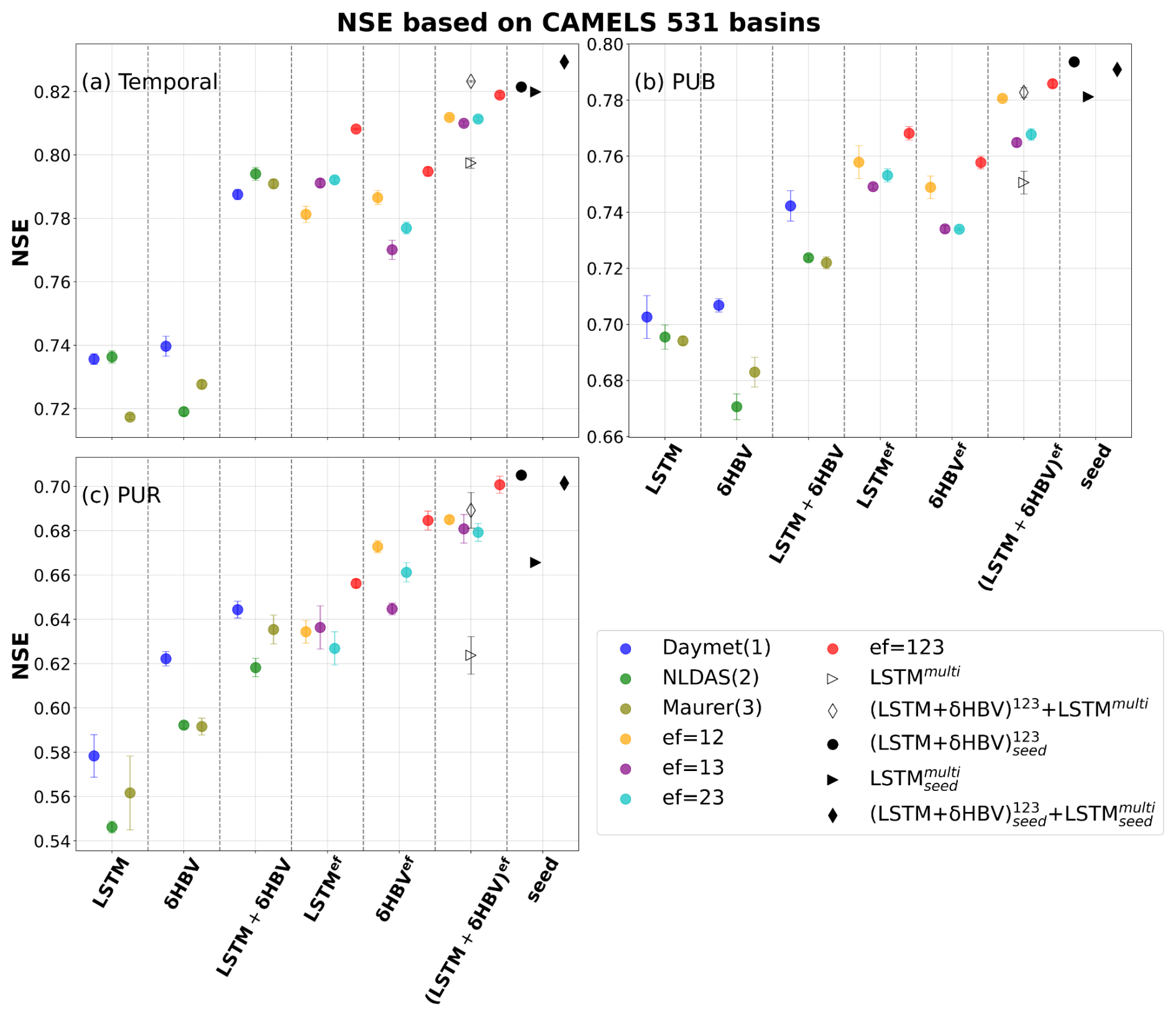
Figure 2 Median NSE values for 531 CAMELS basins, indicating model and ensemble performances for (a) temporal, (b) prediction in ungauged basin (PUB), and (c) prediction in ungauged region (PUR) tests. Different simulations are represented by variously-shaped and -colored points, and are organized by ensemble group, listed along the x-axis: LSTM, δHBV, LSTM + δHBV, and their “ensemble forcing” counterparts, LSTM^ef, δHBV^ef, and (LSTM+δHBV)^ef. LSTM^multi is a single LSTM model trained directly on all three forcing datasets at once. The superscript “ef” denotes the forcing datasets involved in each ensemble (choices of 1 for Daymet, 2 for NLDAS, and 3 for Maurer), while the “+” connects the model types used within an ensemble. The x-axis group and subscript “seed” indicate that simulation results were averaged based on three different random seeds (see Fig. C1). Other points without “seed”, along with their corresponding error bars, are derived from the averages of metrics computed over repeated runs with three different random seeds. The error bar indicates one standard deviation above and below the average value for each simulation.

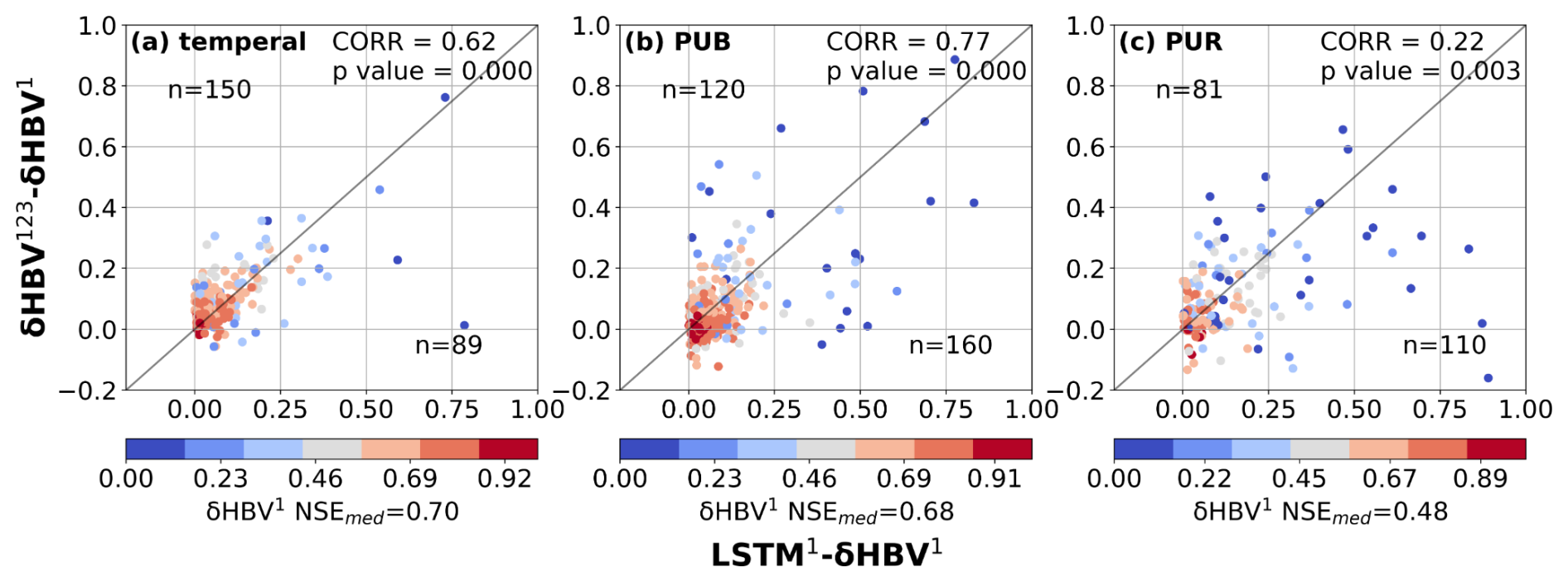
Figure 3 Scatter plots comparing the performance differences between hydrological models for the basins where LSTM outperformed δHBV (the basins where δHBV outperformed are not shown in this plot). The x-axis represents the NSE differences between LSTM¹ and δHBV¹ (LSTM¹−δHBV¹), while the y-axis shows the NSE differences between δHBV¹²³ and δHBV¹ (δHBV¹²³−δHBV¹). Points are color-coded according to the NSE values of δHBV¹. The correlation coefficient (CORR) and p values between the x-axis values and the y-axis values, along with the median NSE value of δHBV¹ (NSE_med) on these basins, are also noted. We note that NSE is not additive and should generally not be subtracted. Here the purpose is only to confirm that basins where LSTM outperforms δHBV also tend to be those that benefit from the ensemble of forcings.

In the lower-performing basins where LSTM¹ had advantages over δHBV¹, the ensemble of meteorological forcings δHBV¹²³ also tended to be higher than δHBV¹ (Fig. 3), suggesting that forcing quality was a significant reason behind the underperformance of δHBV¹ in these basins. Similar patterns were also observed when analyzing δHBV² and δHBV³ values (Figs. D1 and D2 in Appendix D). These basins previously contributed to LSTM's cumulative distribution function of NSE diverging from that of δHBV¹ at the low end (Feng et al., 2022). Forcing errors can exist in the form of systematic timing errors, low or high bias for larger events, etc., which can be difficult for the mass-balanced conceptual HBV¹ structure to adapt to these errors. Because the ensemble of forcings tends to suppress the errors in each forcing source, part of the advantages of δHBV¹²³ over δHBV¹ can be attributed to reducing forcing bias or timing errors. Since the advantages of LSTM¹ over δHBV¹ also tend to occur with these same basins, this also explains how LSTM¹ surpasses δHBV¹ in some basins with poorer-quality forcings. In contrast to δHBV, LSTM has the innate ability to shift information in time and moderately adjust the input scale. Moving from temporal validation to PUB to PUR scenarios, the advantages of diverse forcing datasets appear to diminish, as evidenced by the decreasing ratio of points above versus below the diagonal line, since the forcing error patterns remembered by LSTM may not generalize well in space (discussed in more detail in Sect. 3.2).

Ensembling streamflow simulations from different meteorological forcing datasets demonstrates certain advantages over the previous approach of simultaneously sending multiple forcings into a data-driven model like LSTM (Kratzert et al., 2021). Ensembling LSTM simulations each using a single forcing dataset (LSTM¹²³) resulted in an NSE value of 0.8082, higher than that of 0.7974 from feeding multiple forcing datasets into a single LSTM (LSTM^multi). This difference was more pronounced in the cross-model-type ensemble, after including δHBV, compared to the previous within-class ensemble, and particularly notable for the spatial generalization tests (to be discussed in more detail in Sect. 3.2). The corresponding specific performance metrics are summarized in Tables D1–D5 in Appendix D, with seasonal evaluations provided in Fig. D3. These results indicate that the trained LSTM in LSTM^multi may be overfit to the significant redundant information in these three forcing datasets, and that LSTM models alone cannot fully exploit the information hidden in the multiple forcing datasets. Training separate ensemble members via different nonlinear hydrological processes, on the other hand, seems to allow different bias features to emerge with separate forcing datasets, accordingly mitigating them during the subsequent ensembling process.

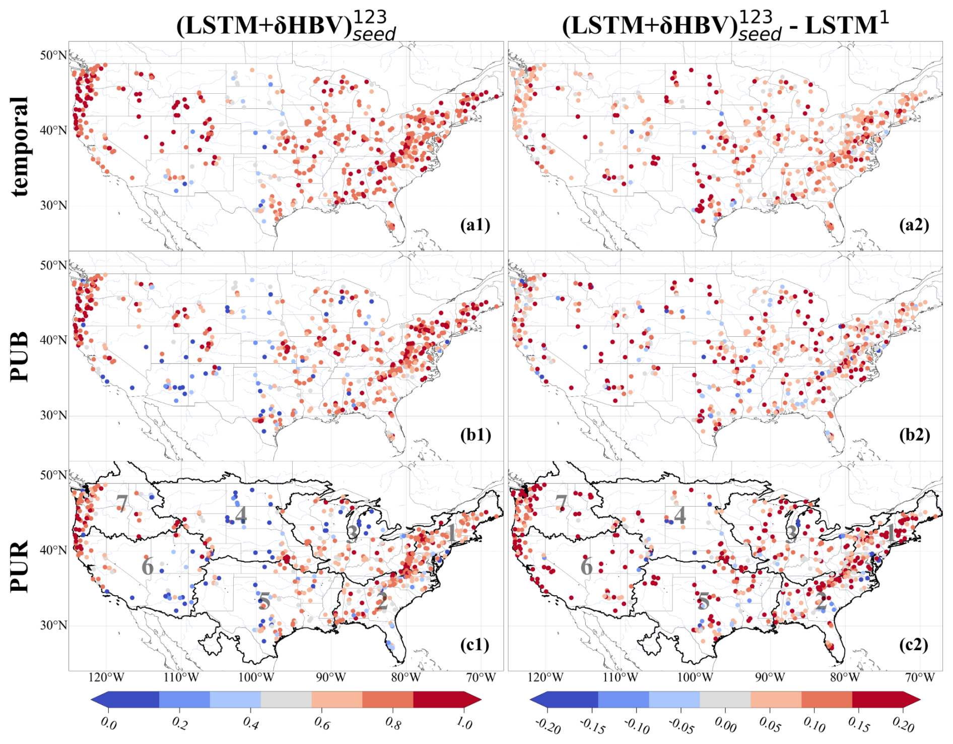
Figure 4 Spatial distributions of NSE values over 531 basins. Subplots are arranged in rows, indicating (a) temporal, (b) PUB, and (c) PUR test results, and columns, denoting (1) NSE values from $(\mathrm{LSTM}+\mathit{\delta }\mathrm{HBV}{)}_{\mathrm{seed}}^{\mathrm{123}}$ and (2) the differences between these NSE values and those of LSTM¹ (models using only forcing 1, Daymet). For LSTM¹ each NSE value reported was the average of three NSE values from three simulations using three different random seeds. The seven continuous regions used to divide up basins for the PUR test are outlined and numbered in the PUR test maps.

Our most diverse ensemble, $(\mathrm{LSTM}+\mathit{\delta }\mathrm{HBV}{)}_{\mathrm{seed}}^{\mathrm{123}}+{\mathrm{LSTM}}_{\mathrm{seed}}^{\mathrm{multi}}$, achieved a median NSE value of ∼ 0.83, surpassing the ∼ 0.82 benchmark set by ${\mathrm{LSTM}}_{\mathrm{seed}}^{\mathrm{multi}}$ (Table D4). This advancement was achieved through random seed variation and cross-model-type ensembling. The performance of (LSTM+δHBV)¹²³ ensemble proved more robust than LSTM^multi, with only a slight boost when we incorporated random seeds, i.e., $(\mathrm{LSTM}+\mathit{\delta }\mathrm{HBV}{)}_{\mathrm{seed}}^{\mathrm{123}}$. Notably, the derived $(\mathrm{LSTM}+\mathit{\delta }\mathrm{HBV}{)}_{\mathrm{seed}}^{\mathrm{123}}$ ensemble outperformed LSTM¹ across almost all basins (Fig. 4). Further incorporation of LSTM^multi into this framework, especially when using multiple random seeds, $(\mathrm{LSTM}+\mathit{\delta }\mathrm{HBV}{)}_{\mathrm{seed}}^{\mathrm{123}}+{\mathrm{LSTM}}_{\mathrm{seed}}^{\mathrm{multi}}$, yielded the best overall performance. Here, the margin over the previous benchmark was small in the temporal test. However, as we will show in Sect. 3.2, the previous benchmark, ${\mathrm{LSTM}}_{\mathrm{seed}}^{\mathrm{multi}}$, lacked robustness, exhibited greater deficiencies in spatial generalization, and negatively impacted ensemble simulations.

When we changed the number of random seeds from 3 to 10, we found that although all model and ensemble performances slightly improved, the gaps between them did not change much (Fig. 5; Table D5 for 10 seeds, Table D4 for 3 seeds). In particular, the gap between $(\mathrm{LSTM}+\mathit{\delta }\mathrm{HBV}{)}_{\mathrm{seed}}^{\mathrm{123}}+{\mathrm{LSTM}}_{\mathrm{seed}}^{\mathrm{multi}}$ and $(\mathrm{LSTM}+\mathit{\delta }\mathrm{HBV}{)}_{\mathrm{seed}}^{\mathrm{123}}$ or ${\mathrm{LSTM}}_{\mathrm{seed}}^{\mathrm{multi}}$ remained unchanged. This indicates that the benefits from more random seeds rapidly become marginal, and our results based on 3 random seeds were sufficiently robust. For LSTMs alone, different random seeds displayed higher variation, and ensembling them led to greater improvement than ensembling (LSTM+δHBV)¹²³ with additional random seeds. It was noteworthy that while the (LSTM+δHBV)¹²³ ensemble generally showed the lowest RMSE values, it did not always show the best high flow performance, as indicated by highRMSE (Tables D1–D4). After incorporating the ${\mathrm{LSTM}}_{\mathrm{seed}}^{\mathrm{multi}}$ variant into $(\mathrm{LSTM}+\mathit{\delta }\mathrm{HBV}{)}_{\mathrm{seed}}^{\mathrm{123}}+{\mathrm{LSTM}}_{\mathrm{seed}}^{\mathrm{multi}}$, overall RMSE and highRMSE both improved. Nevertheless, this ensemble did not always obtain the best values in other metrics like low flow (lowRMSE) and requires further improvement.

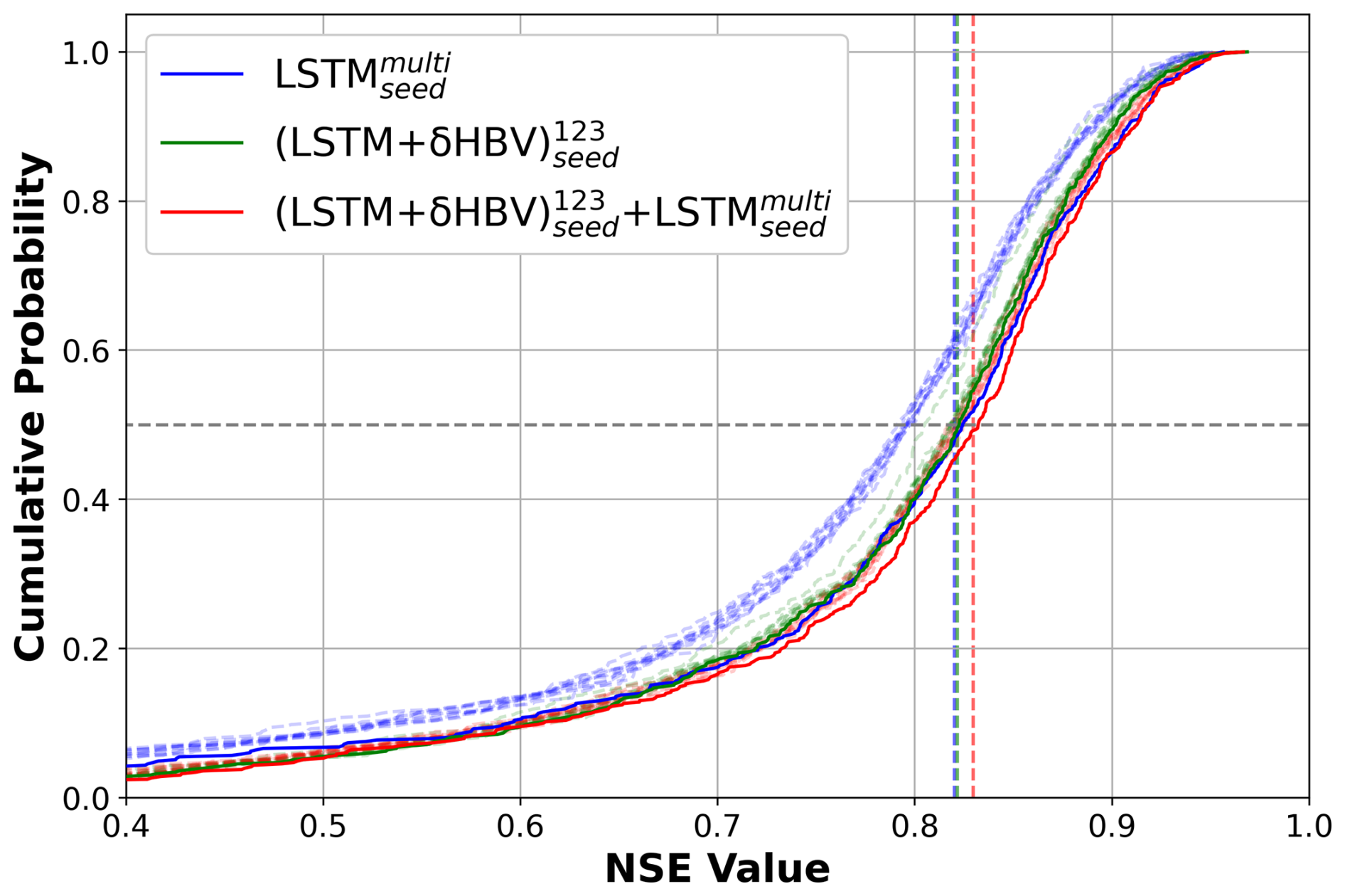
Figure 5 Cumulative distribution function (CDF) curves based on temporal test results for LSTM^multi, (LSTM+δHBV)¹²³, and $\left[\right(\mathrm{LSTM}+\mathit{\delta }\mathrm{HBV}{)}^{\mathrm{123}}+{\mathrm{LSTM}}^{\mathrm{multi}}]$. The solid lines (with “seed”) denote the results with 10 random seeds while the corresponding dashed and translucent lines denote the performances of their individual members each based on one random seed. The median NSE values computed with 3 random seeds are also indicated by vertical dashed and translucent lines in the corresponding colors.

3.2 Spatial generalization

It is clear that cross-model-type ensembling and the incorporation of δHBV significantly improved prediction in ungauged basins (PUB) or regions (PUR), mitigating the difficulty of spatial generalization (Fig. 2b–c). In particular, the previous record-holder for temporal test performance, ${\mathrm{LSTM}}_{\mathrm{seed}}^{\mathrm{multi}}$, incurred large drops in the PUB and PUR tests, once again reminding us of the limitations of LSTM in spatial generalization. Given the same forcings, δHBV-only individual simulations or ensembles consistently outperformed LSTM-only counterparts in the PUR test. Furthermore, adding δHBV to the same-model-type LSTM ensembles improved median NSE by 0.02–0.03 for PUB. The role of δHBV became even more prominent in the harder PUR tests, with an increased gap (0.04–0.07), e.g., LSTM¹²³ (median NSE ∼ 0.656) and (LSTM+δHBV)¹²³ (median NSE ∼ 0.701). The increased significance of δHBV is also illustrated by the optimized weights shown in Fig. E1 in Appendix E, which were estimated using a genetic algorithm with streamflow observations from the test periods. These weights are presented solely to illustrate the relative contributions of the different ensemble components. The significantly different spatial distribution patterns of these weights among different test scenarios also indicate the differences among temporal, PUB, and PUR tests (Figs. E2–E3). The performance of (LSTM+δHBV)¹²³ improved compared to LSTM^multi regardless of whether multiple random seeds were employed to form an ensemble. As such, we can conclude that the inclusion of a differentiable process-based model like δHBV in an ensemble is a systematic way to reduce the risks of failed generalizations of LSTM.

Utilizing a cross-model-type ensemble led to widespread improvements over LSTM-only ensembles, with the exception of a few scattered basins for each temporal (Fig. 4a2), PUB (Fig. 4b2), and PUR (Fig. 4c2) test. The most significant improvements due to the ensemble were concentrated on the center of the Great Plains along with the midwestern US, while the eastern US was moderately improved, suggesting data uncertainty is a larger issue in the central and midwestern US. The Great Plains have historically had poor performance for all kinds of models (Mai et al., 2022) and even the ensemble model had NSE values of only 0.3–0.4 for many of the basins there, although this still marked significant improvements over LSTM¹ (Fig. 4a2, b2, c2). Some western basin NSE values were elevated by more than 0.15 for the temporal test (Fig. 4a2) and even more for PUB and PUR. Meteorological stations are generally sparse on the Great Plains, and an ensemble seems to be an effective way to leverage the different forcing datasets that are available. The poor performances in some basins highlight some remaining deficiencies in current models, which clearly cannot fully consider the heterogeneities of different basins; thus, multiscale formulations that resolve such heterogeneities may have advantages (Song et al., 2025a).

To investigate why ensembles outperformed single-model, single-forcing approaches, we compared their temporal, PUB, and PUR test simulation time series against observations for 531 basins (Fig. 6). Analysis of averaged hydrological year data revealed that while individual ensemble members using single-source forcing datasets performed similarly for easily simulated periods, they showed significant divergence during challenging periods, particularly peak flows. This divergence stems from distinct systematic errors inherent to different model types and forcing datasets. Notably, LSTM-based simulations alone proved insufficient in generating adequate spread to capture these divergent points. By averaging individual model outputs and stabilizing uncertainties, ensemble simulations achieved effective and robust performance across all conditions, which can be shown via the metric highRMSE and lowRMSE values in Tables D1–D4. This highlights the critical importance of comprehensive training for each ensemble member, including diverse forcing inputs, full-period model calibration, and rigorous hyperparameter tuning, to ensure that each member develops distinct simulation behaviors. These differences allow the ensemble to better represent a range of hydrological responses, particularly under extreme or uncertain conditions. By capturing complementary strengths and compensating for individual weaknesses, such well-trained ensemble members collectively enhance the robustness and accuracy of streamflow simulations.

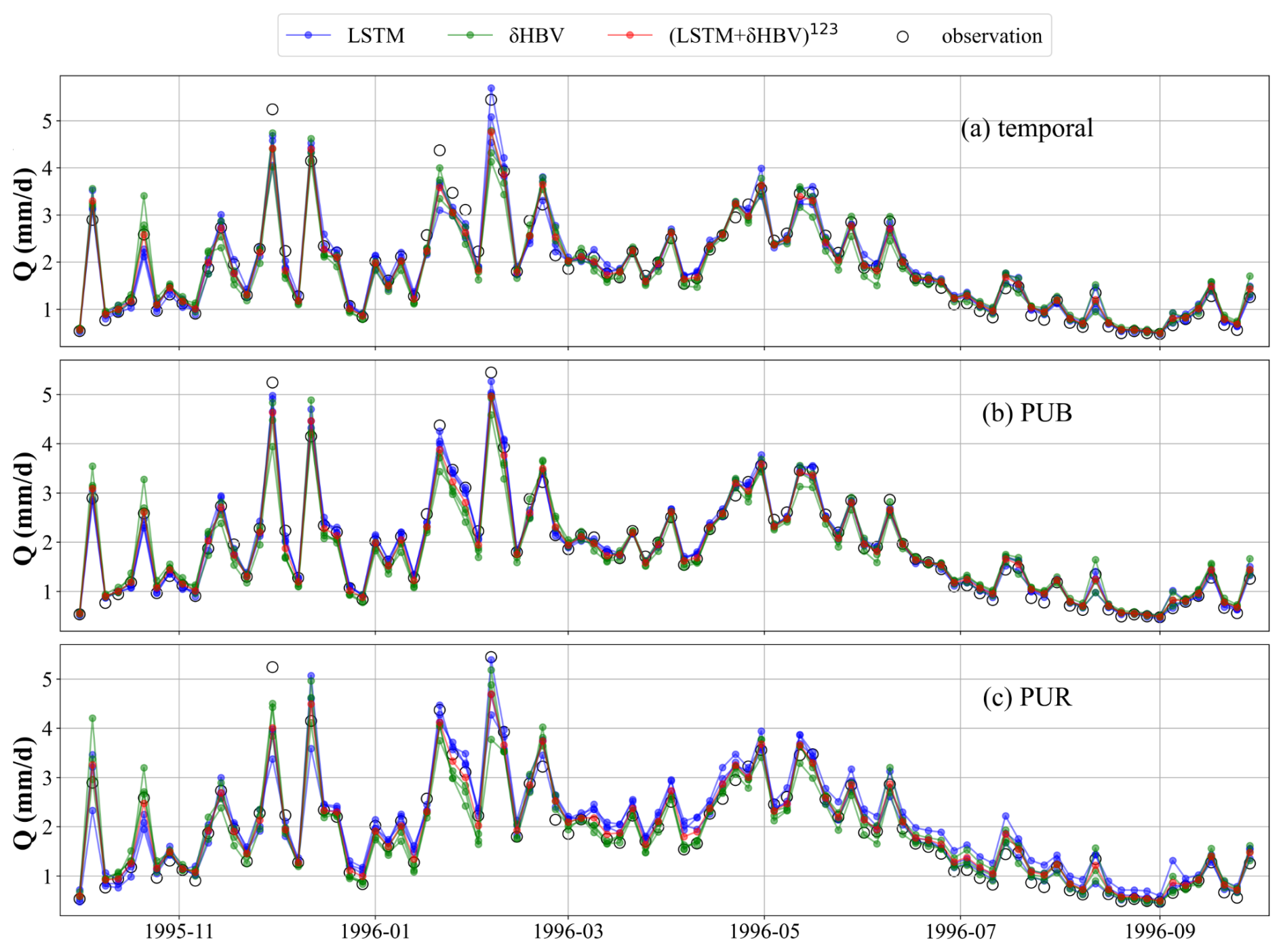
Figure 6 Comparisons between multi-basin-averaged streamflow observations and simulations across 531 basins. The time series points are displayed at four-day intervals for clarity and conciseness. Ensemble members based on the same model (LSTM or δHBV) but driven by different forcing datasets are shown in the same color to highlight the differences between models more clearly.

3.3 Ensemble variability and robustness analysis

Although δHBV (median spread 0.61) exhibits lower spreads than LSTM (mean spread 0.72), their combination increases the ensemble spreads, thereby enhancing diversity (Fig. 7). This pattern holds across the temporal, PUB, and PUR tests. Ensemble effectiveness depends on the diversity of model behaviors and their distinct error characteristics. Consequently, larger spreads are generally associated with greater ensemble benefits. Figure D4 further demonstrates that δHBV + LSTM exhibits larger spreads than LSTM in most basins.

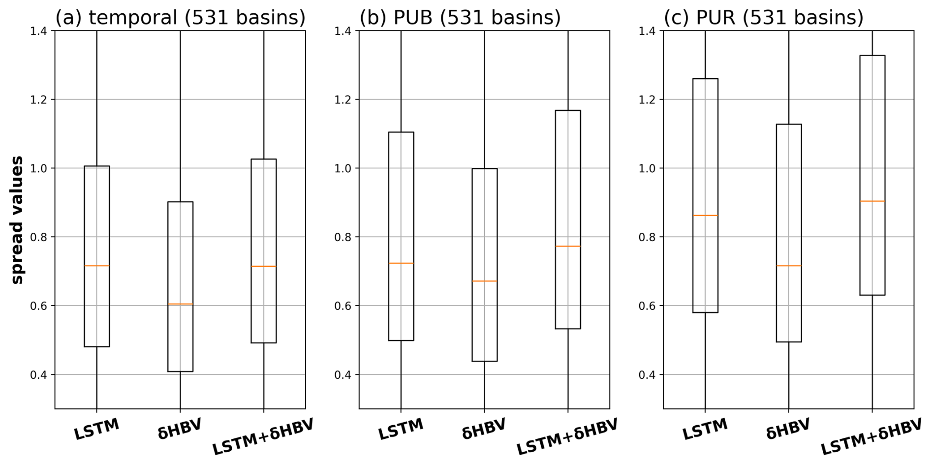
Figure 7 Spread values (Table C2) of each model for LSTM, δHBV, and LSTM + δHBV due to different meteorological forcings and random seeds across temporal, PUB, and PUR tests.

As the warming signal is already clear across most basins under any forcing across the periods of simulation (Fig. D5), the models' strong performance in the temporal test suggests decent extrapolation capability under warming scenarios. It is often questioned whether data-driven models like LSTM lose accuracy under stronger climate drift, but no substantially warmed dataset is available to test this. Benchmarks suggest LSTM captures 15-year trends well in temporal tests, but less so in data-sparse scenarios (Feng et al., 2023b). Introducing a 10 % precipitation perturbation (multiplying precipitation by 1.1) slightly reduced performance for both models as expected (Fig. D6a and b), but ensemble benefits remained robust across models despite the perturbation.

Training sample size, dynamic parameter choices, and lookback windows exert only a limited impact on our conclusions. δHBV shows limited sensitivity to sample size, with similar results when trained on 531 versus 671 basins (Fig. D6c). Regarding parameter uncertainties, fixing one δHBV parameter (k₀) as static increased structural errors and reduced performance (Fig. D6d), yet ensemble benefits remained robust. For LSTM, alternative window sizes of 182 and 730 d were tested, with the default 365 d window yielding optimal performance (Fig. D6e). Importantly, variations in the lookback window had only minor effects on model performance, underscoring the robustness of ensemble benefits.

3.4 Further discussion

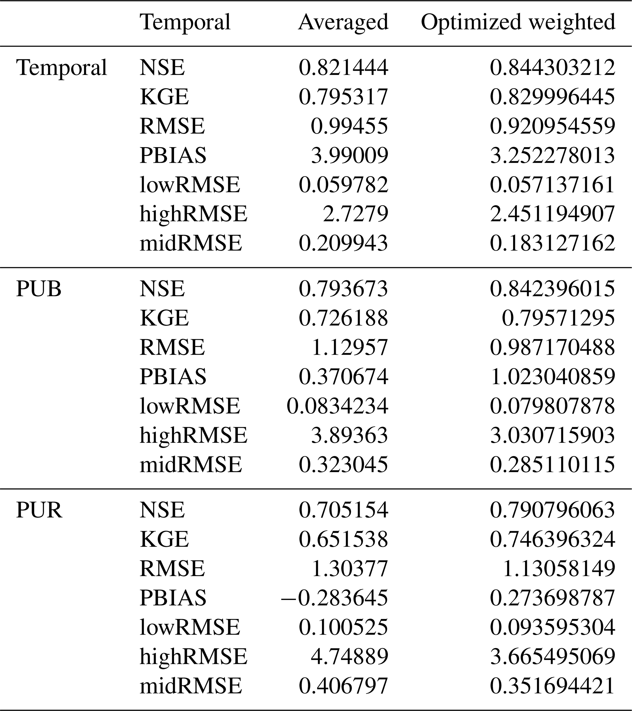
Based on our results, we identified several avenues for future research. First, while we have explored various weighting strategies and found that averaging yields the best performance yet, we believe that dynamic or adaptive weighting schemes could further enhance performance in future studies. It is also demonstrated by Table E1 that estimated uneven weights can significantly improve simulation performance. Moreover, within specific basins, the estimated weights of different components are often highly imbalanced, as evidenced by the spatial distribution of optimized weights (Figs. E2–E3). Some potential feasible ways include using the simulations from these individually-trained models as inputs of a data-driven model (Solanki et al., 2025), and making the weight estimation and the ensemble member training simultaneously.

Both LSTM and δHBV models exhibit limitations in regions with significant anthropogenic impacts, such as dam presence, as well as arid climatic and highly heterogeneous geological conditions. These regions are mainly located in the midwestern and western CONUS, where high evaporation conditions (Heidari et al., 2020) and numerous dams (Bellmore et al., 2017) coincide with complex water use processes (Wada et al., 2016) that current models cannot simulate well. Together, these factors suggest that anthropogenic influence is likely an important driver of poor model performance. Further improvements may include incorporating additional data that capture these factors like capacity-to-runoff ratio (Ouyang et al., 2021) or integrating specialized modules, such as reservoirs (Hanazaki et al., 2022; West et al., 2025). Compared with LSTM, δHBV is more sensitive to precipitation biases. For example, the differences between δHBV simulations under different forcing datasets were generally larger than those for LSTM, and δHBV using the Daymet forcing dataset showed largely better performance than with the other two forcing datasets, which indicates that δHBV may not be able to fit different forcing datasets well. Therefore, many potential structural optimizations can be implemented to improve δHBV. Our analysis provided corroborating evidence that forcing error is an important reason why LSTM can outperform δHBV in the temporal test for some basins, although such patterns may not generalize well in space. A meteorological forcing data correction module can be developed in the future to account for timing and magnitude errors in precipitation. Ensemble simulations may face challenges when computational resources are constrained, particularly for large-scale or real-time applications. Nevertheless, we remain optimistic about overcoming these challenges due to several promising solutions. These include tailoring the hydrological model by simplifying less relevant components to specific simulation objectives (Clark et al., 2015; Kraft et al., 2022) and cloud-based computing infrastructures that offer scalable, on-demand resource allocation (He et al., 2024; Leube et al., 2013). Importantly, the majority of computational costs are incurred during model training. In practice, ensemble members are typically pre-trained by different research or application groups (Bodnar et al., 2025; Nearing et al., 2024; Song et al., 2025a), enabling direct reuse of these well-trained models and significantly improving computational efficiency.

For this work, we did not create a δHBV^multi model (in the same vein as LSTM^multi) using all forcings as an input to a single model, since a similar experiment has already been conducted by Sawadekar et al. (2025). We also did not examine “seed” combinations of a δHBV^multi as we believed they would not result in a significant performance boost (unlike that seen with LSTM^multi), because LSTM has high variability and low bias, while δHBV has lower variance and potentially higher bias. As a result, random seeds would likely not create large enough perturbations for δHBV and wouldn't bring the benefits seen with ${\mathrm{LSTM}}_{\mathrm{seed}}^{\mathrm{multi}}$. To achieve an equivalent perturbation level for δHBV, it may be necessary to incorporate multiple distinct hydrological models, such as SAC-SMA, PRMS, and GR4J, similar to the approach implemented in the Framework for Understanding Structural Errors (FUSE) (Clark et al., 2008). Work is ongoing to create a combination of a series of differentiable process-based models, which is expected to produce a further improved ensemble with great interpretability. Given the success of cross-model-type ensembles shown in this work, we also encourage further exploration of ensemble simulations involving models with other distinct mechanisms.

4 Summary and conclusions

This study comprehensively analyzes ensemble combinations of two advanced model types (LSTM and δHBV), each with distinct mechanisms, for streamflow simulation across 531 basins in the US. Three meteorological forcing datasets (Daymet, NLDAS, and Maurer) are employed to fully capture the characteristics of the two models. Their applications are also tested in two distinct ways: (1) by feeding all diverse forcing datasets simultaneously into a single LSTM model, and (2) by ensembling the outputs of multiple LSTM models, each trained separately using a single forcing dataset. The performance of ensemble simulations was evaluated under three distinct testing scenarios (temporal, PUB, and PUR tests), surpassing the previous highest performances. Our findings enhance the understanding of how to effectively utilize diverse model types and multi-source datasets to improve streamflow simulations. The principal conclusions are:

1. Cross-model-type ensembles (LSTM + δHBV) consistently outperformed single-model approaches across all test scenarios, setting new performance benchmarks on the CAMELS dataset. These ensembles demonstrated the complementarity of data-driven (LSTM) and physics-informed (δHBV) approaches in capturing diverse hydrological behaviors.

2. Ensembling models trained on different forcing datasets proved more effective than using multiple forcing datasets as simultaneous inputs to a single model. This suggests that separate training allows each model to capture unique features contained in each forcing dataset, which can then be effectively leveraged in the ensemble.

3. δHBV provided significant benefits to ensemble simulations on spatial generalization. Ensembling LSTM with δHBV showed increasing benefits as generalization challenges increased, from temporal to spatial interpolation (PUB) to spatial extrapolation (PUR) tests. This underscores the value of physics-informed constraints in improving model transferability to ungauged basins and regions.

4. While ensemble methods significantly improved overall performance, they did not fully mitigate consistent deficiencies in certain challenging areas (e.g., regions with high dam density or heterogeneous hydrogeological conditions). This indicates areas for future model development.

These findings have important implications for hydrological modeling and water resources management. The improved accuracy and spatial generalization of our ensemble approach can enhance streamflow predictions, benefiting water resources planning and management, particularly in data-scarce regions. Our results also suggest that future hydrological model development should focus on combining data-driven and physics-based approaches to improve model generalizability across diverse conditions. The superior performance of ensembling models with different forcing datasets over using merged forcings as a single input highlights the risk of indiscriminately feeding all available data into one data-driven model. While computational demands certainly require consideration, the potential improvements in prediction accuracy offer significant value for both research and operational applications. Future work should focus on refining these ensemble techniques, addressing model limitations in challenging regions, and exploring ensemble implementation in operational settings.

Appendix A: Detailed processes of HBV employed in this study

The Hydrologiska Byråns Vattenbalansavdelning (HBV) model (Aghakouchak and Habib, 2010; Beck et al., 2020; Bergström, 1976, 1992) is a simple yet effective bucket-type hydrologic model that simulates hydrologic components including snow water equivalent, soil moisture, groundwater storage, evapotranspiration, quick flow, baseflow, and total streamflow.

In the following, we describe these processes in detail with their corresponding equations. Uppercase letters denote state variables, while lowercase letters denote parameters. The overall water balance is expressed as Eq. (A1).

$$\begin{array}{}\text{(A1)}& \mathrm{EP}-\mathrm{AE}-Q_{\mathrm{t}}=\mathrm{SN}+\mathrm{SM}+\mathrm{SUZ}+\mathrm{SLZ}+\mathrm{LAKE}\end{array}$$

where EP is effective precipitation, AE is actual evapotranspiration, Q_t is total simulated runoff, SN is snow storage, SM is soil moisture storage, SUZ and SLZ are the upper and lower groundwater storages, respectively, and LAKE represents lake storage (omitted in this study).

First, effective precipitation (EP) is partitioned into rain (RN) and snow (SN) components based on the air temperature (T) relative to a threshold temperature (tt):

$$\begin{array}{}\text{(A2)}& {\displaystyle }\mathrm{RN}=\mathrm{EP}\mathrm{if}T\ge \mathrm{tt}\text{(A3)}& {\displaystyle }\mathrm{SN}=\mathrm{EP}\mathrm{if}T<\mathrm{tt}\end{array}$$

Snow (SN) accumulates in the snowpack (SNP), while snowmelt (SNM) happens when T≥tt, which is calculated based on a melt factor (cfm) and the temperature difference (T−tt). The computed snowmelt (SNM) is constrained by the available snowpack (SNP).

$$\begin{array}{}\text{(A4)}& \mathrm{SNM}=min[max\left(\mathrm{cfm}\cdot \left(T-\mathrm{tt}\right),\mathrm{0}\right)\mathrm{SNP}]\end{array}$$

The snowmelt (SNM) contributes to meltwater (MW), while the snowpack (SNP) is updated as:

$$\begin{array}{}\text{(A5)}& {\displaystyle }\mathrm{MW}=\mathrm{MW}+\mathrm{SNM}\text{(A6)}& {\displaystyle }\mathrm{SNP}=\mathrm{SNP}+\mathrm{SN}-\mathrm{SNM}\end{array}$$

A portion of the meltwater (MW) may refreeze when T<tt, controlled by the refreezing parameter (cfr):

$$\begin{array}{}\text{(A7)}& {\displaystyle }\mathrm{RFZ}=min\left[max\left(\mathrm{cfr}\cdot \mathrm{cfm}\cdot \left(\mathrm{tt}-T\right),\mathrm{0}\right),\mathrm{MW}\right]\text{(A8)}& {\displaystyle }\mathrm{SNP}=\mathrm{SNP}+\mathrm{RFZ}\text{(A9)}& {\displaystyle }\mathrm{MW}=\mathrm{MW}-\mathrm{RFZ}\end{array}$$

The remaining meltwater (MW) exceeding the snowpack's liquid water holding capacity (cwh⋅SNP) infiltrates into the soil (IF), with the remainder retained in MW:

$$\begin{array}{}\text{(A10)}& {\displaystyle }\mathrm{IF}=max\left(\mathrm{MW}-\mathrm{cwh}\cdot \mathrm{SNP},\mathrm{0}\right)\text{(A11)}& {\displaystyle }\mathrm{MW}=\mathrm{MW}-\mathrm{IF}\end{array}$$

The fraction of soil moisture (SM) relative to the field capacity (fc), raised to the power index β, modulates shallow seepage (SP) according to the available water (IF+RN):

$$\begin{array}{}\text{(A12)}& {\displaystyle }\mathrm{SP}={\left({\displaystyle \frac{\mathrm{SM}}{\mathrm{fc}}}\right)}^{\mathit{\beta }}(\mathrm{IF}+\mathrm{RN})\text{(A13)}& {\displaystyle }\mathrm{SM}=\mathrm{SM}+\mathrm{IF}+\mathrm{RN}-\mathrm{SP}\end{array}$$

Excess soil water above the field capacity contributes to direct infiltration (IF_dir):

$$\begin{array}{}\text{(A14)}& {\displaystyle }{\mathrm{IF}}_{\mathrm{dir}}=max\left(\mathrm{SM}-\mathrm{fc},\mathrm{0}\right)\text{(A15)}& {\displaystyle }\mathrm{SM}=\mathrm{SM}-{\mathrm{IF}}_{\mathrm{dir}}\end{array}$$

Actual evapotranspiration (AE) is estimated as the product of potential evapotranspiration (PE) and an evapotranspiration coefficient (PEC). The PEC depends on soil moisture storage (SM), field capacity (fc), a shape parameter (λ), and a threshold parameter (lp).

$$\begin{array}{}\text{(A16)}& {\displaystyle }\mathrm{PEC}=min\left[\mathrm{1},max\left(\mathrm{0},{\left({\displaystyle \frac{\mathrm{SM}}{\mathrm{lp}\cdot \mathrm{fc}}}\right)}^{\mathit{\lambda }}\right)\right]\text{(A17)}& {\displaystyle }\mathrm{AE}=\min \left(\mathrm{PE}\cdot \mathrm{PEC},\mathrm{SM}\right)\text{(A18)}& {\displaystyle }\mathrm{SM}=\mathrm{SM}-\mathrm{AE}\end{array}$$

Capillary rise (CP) from the lower zone (SLZ) replenishes SM, controlled by a coefficient (c) and constrained by the soil moisture deficit:

$$\begin{array}{}\text{(A19)}& {\displaystyle }\mathrm{CP}=min\left[c\cdot \mathrm{SLZ}\cdot \left(\mathrm{1}-{\displaystyle \frac{\mathrm{SM}}{\mathrm{fc}}}\right),\mathrm{SLZ}\right]\text{(A20)}& {\displaystyle }\mathrm{SM}=\mathrm{SM}+\mathrm{CP}\text{(A21)}& {\displaystyle }\mathrm{SLZ}=\mathrm{SLZ}-\mathrm{CP}\end{array}$$

Recharge from the soil, consisting of shallow seepage (SP) and direct infiltration (IF_dir), enters the upper groundwater zone (SUZ). Water in the upper zone either percolates to the lower groundwater zone (SLZ) at a constant percolation rate (prc) or contributes to direct runoff (Q₀) when the upper zone (SUZ) exceeds a threshold (uzl). Flow from the upper and lower zones is computed using linear reservoir formulations, with parameters k₀, k₁, k₂ controlling the respective runoff components Q₀, Q₁, Q₂. The total simulated streamflow (Q_t) is then computed as the sum of these components.

$$\begin{array}{}\text{(A22)}& {\displaystyle }\mathrm{SUZ}=\mathrm{SUZ}+\mathrm{SP}+{\mathrm{IF}}_{\mathrm{dir}}\text{(A23)}& {\displaystyle }\mathrm{PERC}=min\left(\mathrm{prc},\mathrm{SUZ}\right)\text{(A24)}& {\displaystyle }\mathrm{SUZ}=\mathrm{SUZ}-\mathrm{PERC}\text{(A25)}& {\displaystyle }{Q}_{\mathrm{0}}=max\left[k_{\mathrm{0}}\cdot \left(\mathrm{SUZ}-\mathrm{uzl}\right),\mathrm{0}\right]\text{(A26)}& {\displaystyle }\mathrm{SUZ}=\mathrm{SUZ}-Q_{\mathrm{0}}\text{(A27)}& {\displaystyle }{Q}_{\mathrm{1}}=\mathrm{SUZ}\cdot k_{\mathrm{1}}\text{(A28)}& {\displaystyle }\mathrm{SUZ}=\mathrm{SUZ}-Q_{\mathrm{1}}\text{(A29)}& {\displaystyle }\mathrm{SLZ}=\mathrm{SLZ}+\mathrm{PERC}\text{(A30)}& {\displaystyle }{Q}_{\mathrm{2}}=\mathrm{SLZ}\cdot k_{\mathrm{2}}\text{(A31)}& {\displaystyle }\mathrm{SLZ}=\mathrm{SLZ}-Q_{\mathrm{2}}\text{(A32)}& {\displaystyle }{Q}_{\mathrm{t}}=Q_{\mathrm{0}}+Q_{\mathrm{1}}+Q_{\mathrm{2}}\end{array}$$

Finally, a routing module (Feng et al., 2022) is used to process Q_t to produce the final streamflow output ($Q_{\mathrm{t}}^{\ast }$). This module with two parameters (θ_α, θ_τ) assumes a gamma function for the unit hydrograph and convolves the unit hydrograph with the runoff as,

$$\begin{array}{}\text{(A33)}& {\displaystyle }{Q}_{\mathrm{t}}^{\ast }=\underset{\mathrm{0}}{\overset{\mathrm{tmax}}{\int }}\mathit{\xi }(s:{\mathit{\theta }}_{\mathit{\alpha }},{\mathit{\theta }}_{\mathit{\tau }})\cdot Q(t-s)\mathrm{d}s\text{(A34)}& {\displaystyle }\mathit{\xi }(s:{\mathit{\theta }}_{\mathit{\alpha }},{\mathit{\theta }}_{\mathit{\tau }})={\displaystyle \frac{\mathrm{1}}{\mathrm{\Gamma }\left({\mathit{\theta }}_{\mathit{\alpha }}\right){\mathit{\theta }}_{\mathit{\tau }}^{{\mathit{\theta }}_{\mathit{\alpha }}}}}{s}^{{\mathit{\theta }}_{\mathit{\alpha }}-\mathrm{1}}{e}^{-\frac{s}{{\mathit{\theta }}_{\mathit{\tau }}}}\end{array}$$

Appendix B: Illustrated differences among the three meteorological forcing datasets

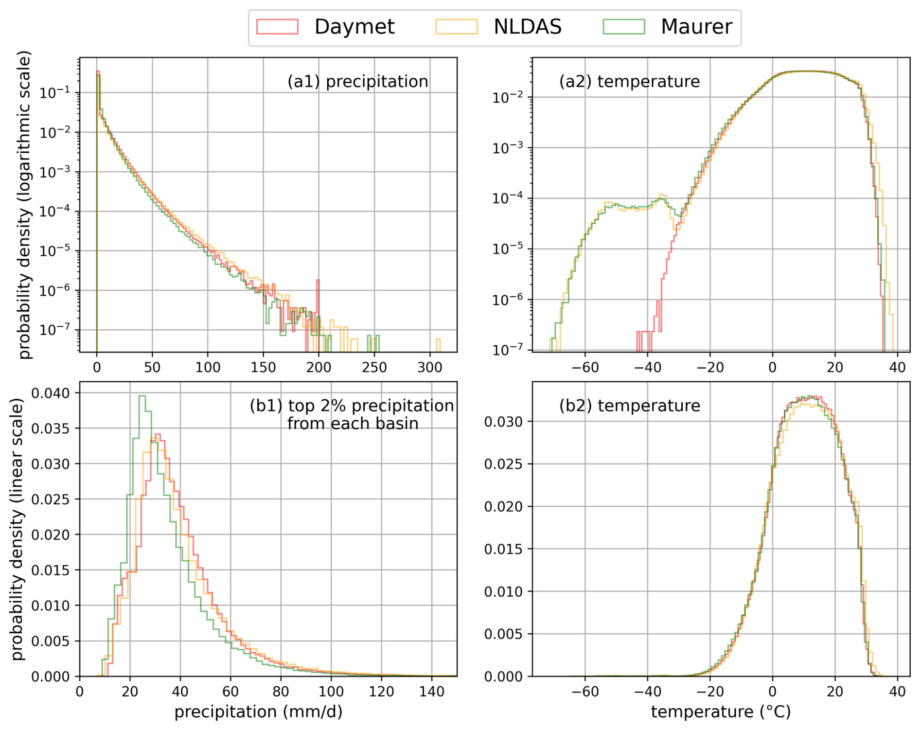
Figure B1 Probability density distributions (top panel in logarithmic scale, bottom panel in linear scale) of precipitation and temperature across three meteorological forcing datasets.

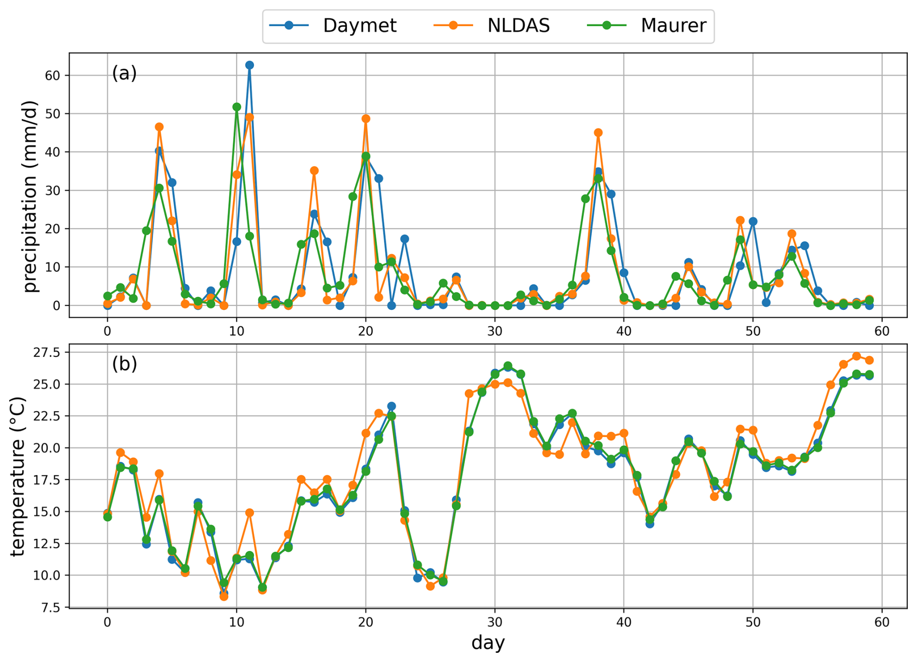
Figure B2 Illustrated temporal variations of precipitation and temperature in a basin across three meteorological forcing datasets.

Appendix C: Details of model inputs, ensemble frameworks, and evaluations

Table C1 Full names for the abbreviations of dynamic data (all but streamflow are “forcings”) and static basin attributes used as model inputs and outputs. All variables and their values are provided in the CAMELS dataset (Addor et al., 2017) except for the NLDAS and Maurer daily temperature extrema, which are from Kratzert et al. (2021). Potential evapotranspiration and normalized streamflow were calculated in this work, using CAMELS data. The number in parentheses specifies model usage: 1 denotes use in the LSTM model, and 2 denotes use in the δHBV model.

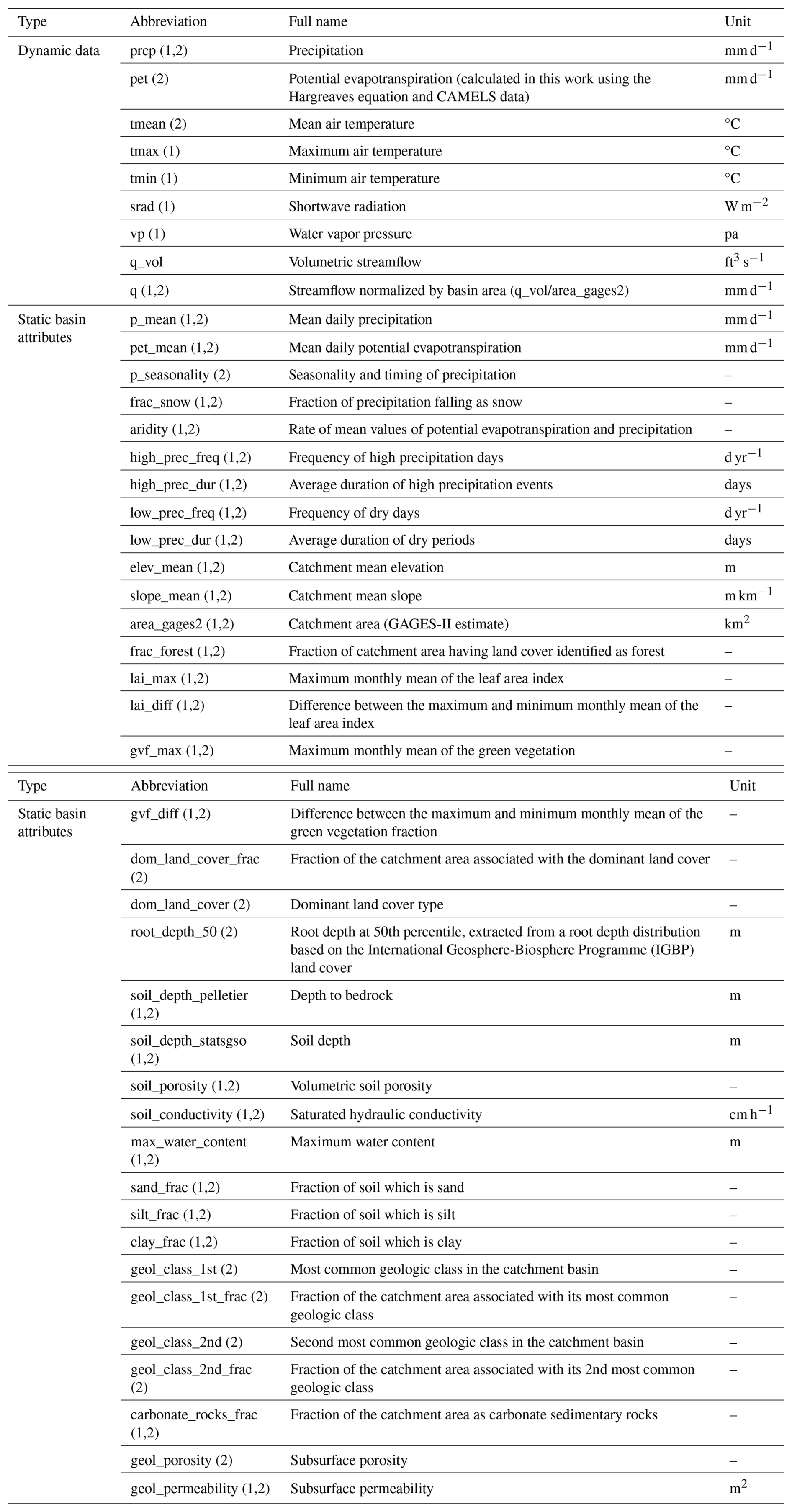
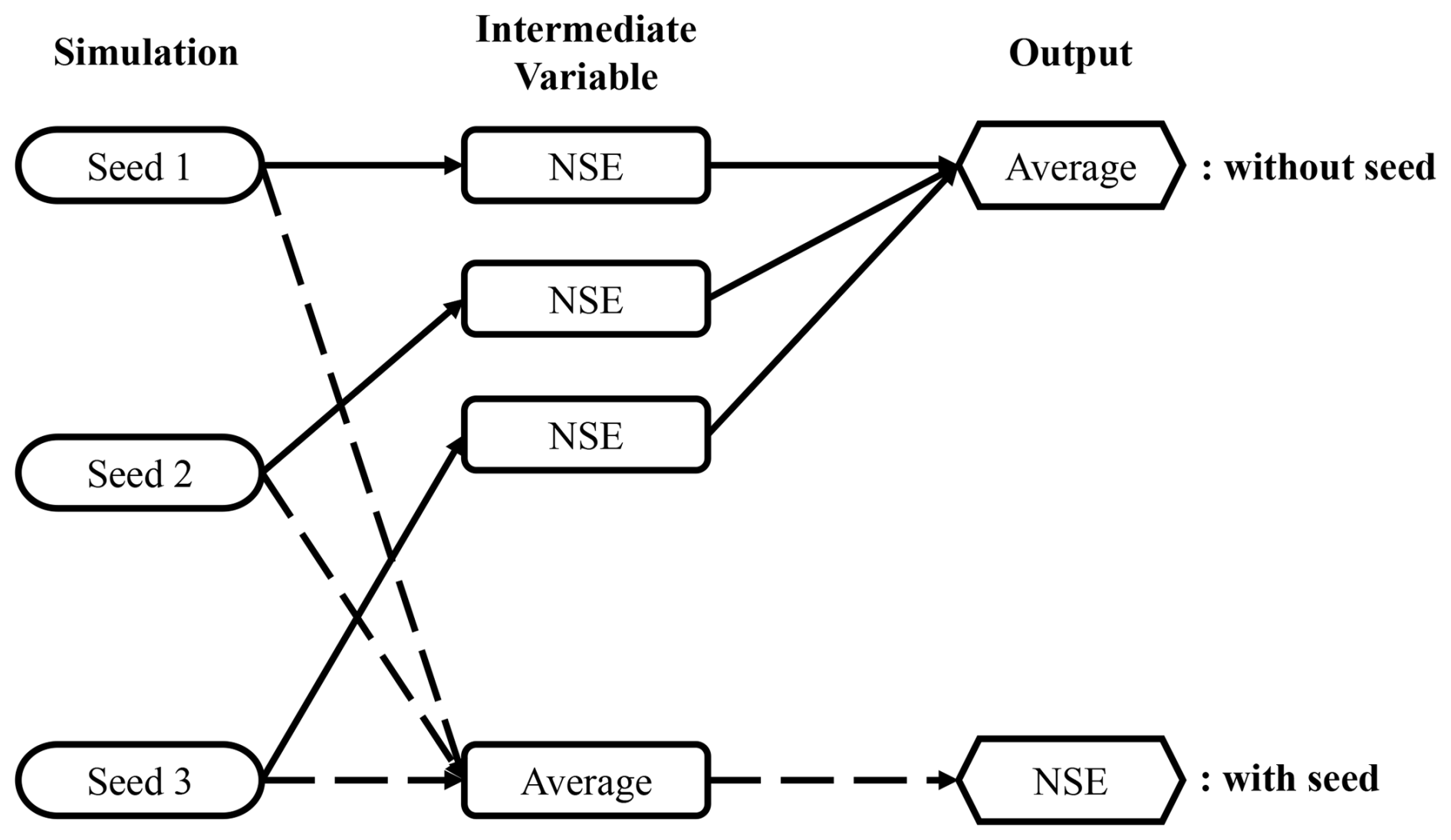
Figure C1 Ensemble frameworks to generate metrics for ensembles named without (solid arrows) and with (dashed arrows) “seed” as a subscript.

Table C2 Loss function and evaluation metrics.

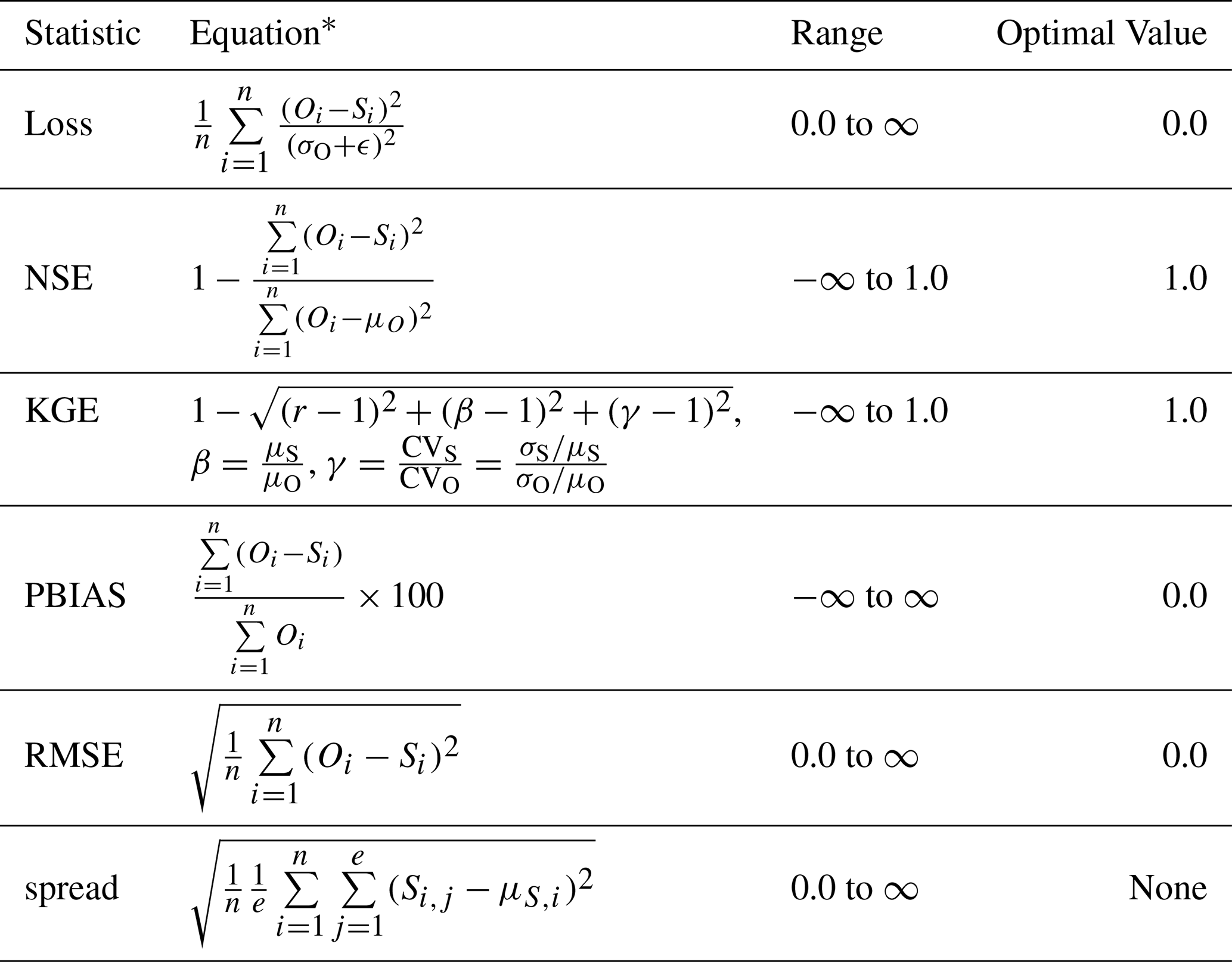
^* S is a streamflow simulation; O is the corresponding observation; n is the number of total S or O; ϵ is a numerical stabilizer, with a default value of 0.1; e is the number of ensemble members; r is the linear Pearson correlation between S and O; β is the mean bias; and γ is the variability bias. The mean and standard deviation of simulations are denoted as μ_S and σ_S, respectively, and μ_O and σ_O are the mean and standard deviation of the observations.

Appendix D: Additional details on model performance

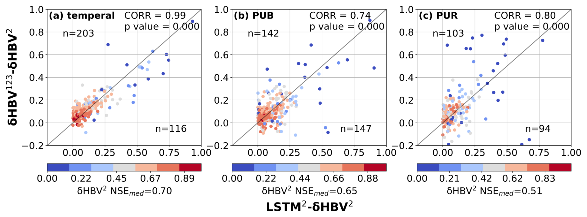
Figure D1 Scatter plots comparing the performance differences between hydrological models for the basins where LSTM outperformed δHBV (the basins where δHBV outperformed are not shown in this plot). The x-axis represents the NSE differences between LSTM² and δHBV² (LSTM²−δHBV²), while the y-axis shows the NSE differences between δHBV¹²³ and δHBV² (δHBV¹²³−δHBV²). Points are color-coded according to the NSE values of δHBV². The correlation coefficient (CORR) and p values between the x-axis values and the y-axis values, along with the median NSE value of δHBV² (NSE_med) on these basins, are also noted.

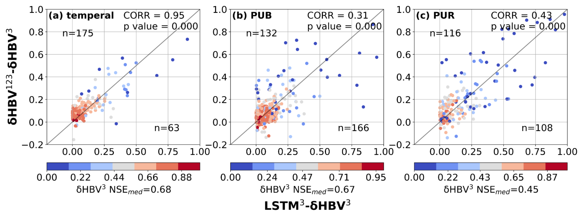
Figure D2 Scatter plots comparing the performance differences between hydrological models for the basins where LSTM outperformed δHBV (the basins where δHBV outperformed are not shown in this plot). The x-axis represents the NSE differences between LSTM³ and δHBV³ (LSTM³−δHBV³), while the y-axis shows the NSE differences between δHBV¹²³ and δHBV³ (δHBV¹²³−δHBV³). Points are color-coded according to the NSE values of δHBV³. The correlation coefficient (CORR) and p values between the x-axis values and the y-axis values, along with the median NSE value of δHBV³ (NSE_med) on these basins, are also noted.

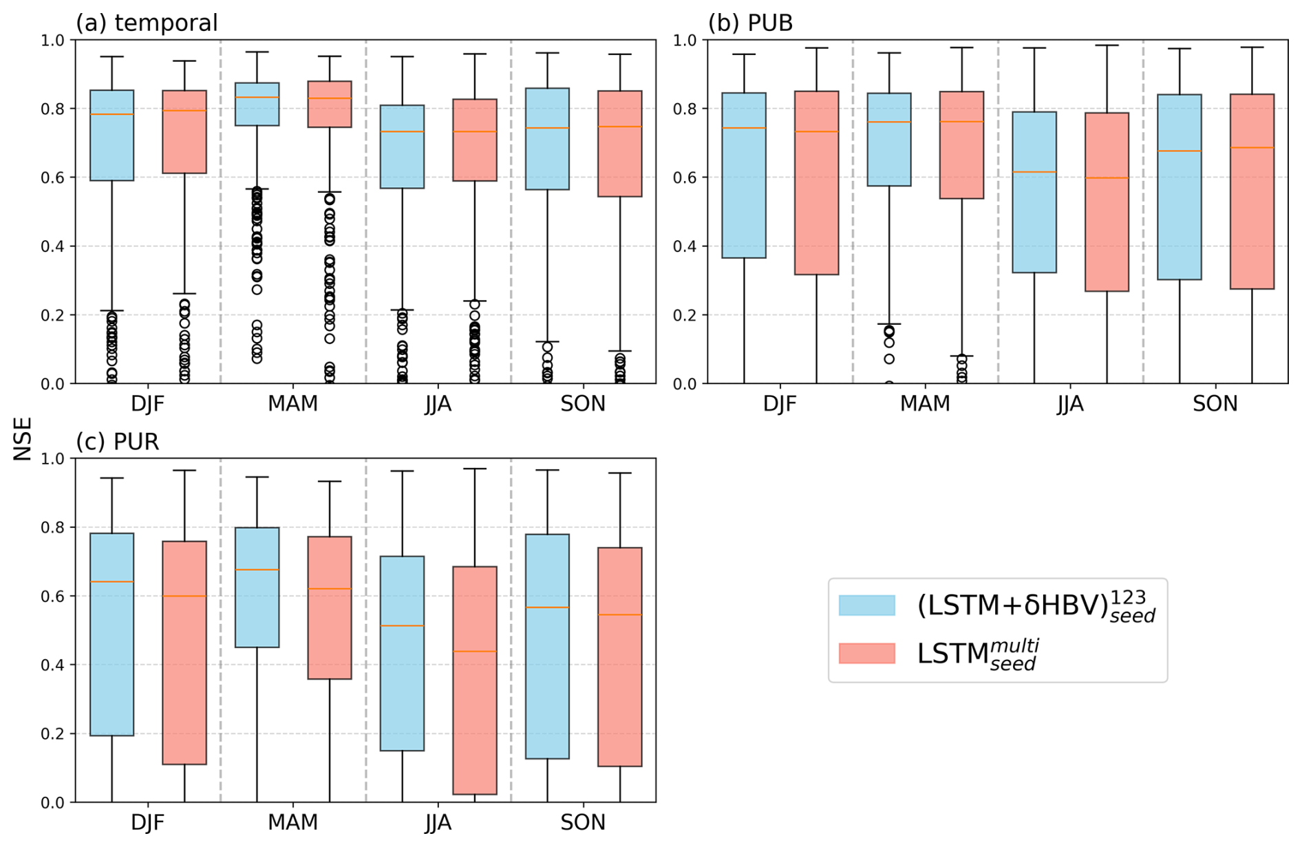
Figure D3 Seasonal comparison of Nash–Sutcliffe efficiency (NSE) values for $(\mathrm{LSTM}+\mathit{\delta }\mathrm{HBV}{)}_{\mathrm{seed}}^{\mathrm{123}}$ (blue) and ${\mathrm{LSTM}}_{\mathrm{seed}}^{\mathrm{multi}}$ (red) in (a) temporal, (b) PUB, and (c) PUR tests. Each box represents the distribution of NSE values across 531 basins for a given season (DJF: December–February, MAM: March–May, JJA: June–August, SON: September–November). Vertical dashed lines separate different seasons. $(\mathrm{LSTM}+\mathit{\delta }\mathrm{HBV}{)}_{\mathrm{seed}}^{\mathrm{123}}$ performs better than ${\mathrm{LSTM}}_{\mathrm{seed}}^{\mathrm{multi}}$ in most cases, especially during MAM, likely due to differences in snowmelt representation.

Figure D4 Spatial distributions of model spread values increase from δHBV and LSTM to the LSTM + δHBV ensemble across temporal, PUB, and PUR tests.

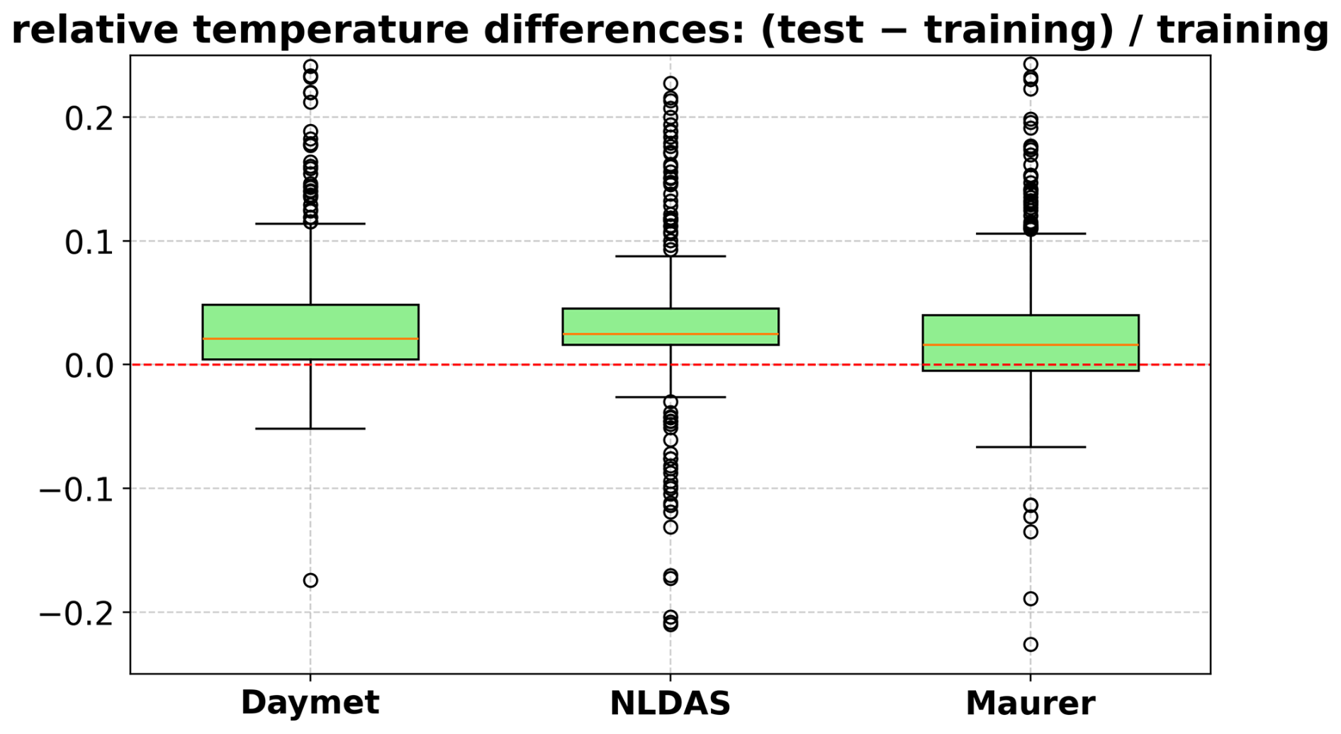
Figure D5 Boxplot of relative temperature differences between the test and training periods, calculated as (test − training)$/$training. Each box represents the distribution of normalized temperature changes across basins for a specific meteorological forcing dataset: Daymet, NLDAS, and Maurer. Positive values indicate warming in the test period relative to the training period.

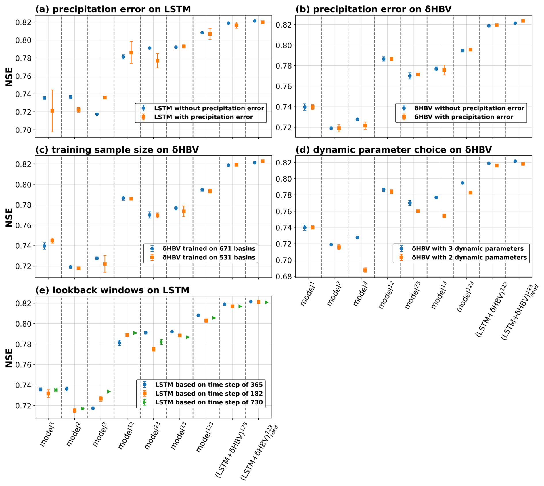
Figure D6 Simulation performance (NSE) under the temporal test: (a) LSTM model with and without a 10 % precipitation error (precipitation × 1.1); (b) δHBV model with and without a 10 % precipitation error; (c) δHBV model trained on 671 versus 531 basins; (d) δHBV model with 3 versus 2 dynamic parameters; (e) δHBV model using time steps of 365, 182, and 730 d. Individual and ensemble groups are distinguished along the x-axis. Ensemble benefits are indicated by the gap between columns of the same color within each panel–columns 1–7 correspond to individual LSTM or δHBV groups, and the last two columns correspond to LSTM + δHBV ensembles.

Table D1 Median NSE, KGE, RMSE, PBIAS, and RMSE values under low (lowRMSE), high (highRMSE), and middle (midRMSE) flows based on 531 basins under the temporal test. The values are the mean of three simulations run with different random seeds.

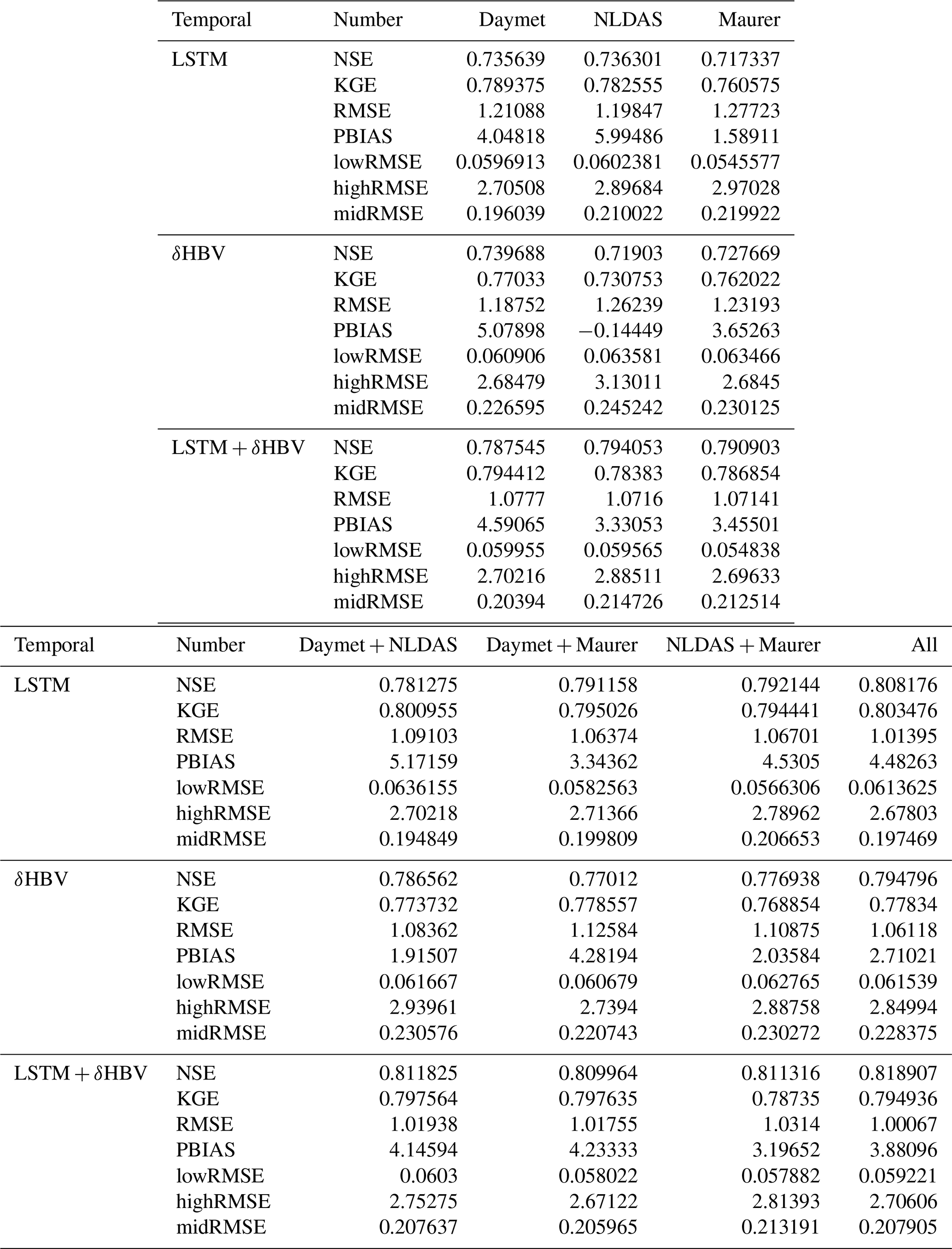
Table D2 Median NSE, KGE, RMSE, PBIAS, and RMSE values under low (lowRMSE), high (highRMSE), and middle (midRMSE) flows based on 531 basins under the PUB test. The values are the mean of three simulations run with different random seeds.

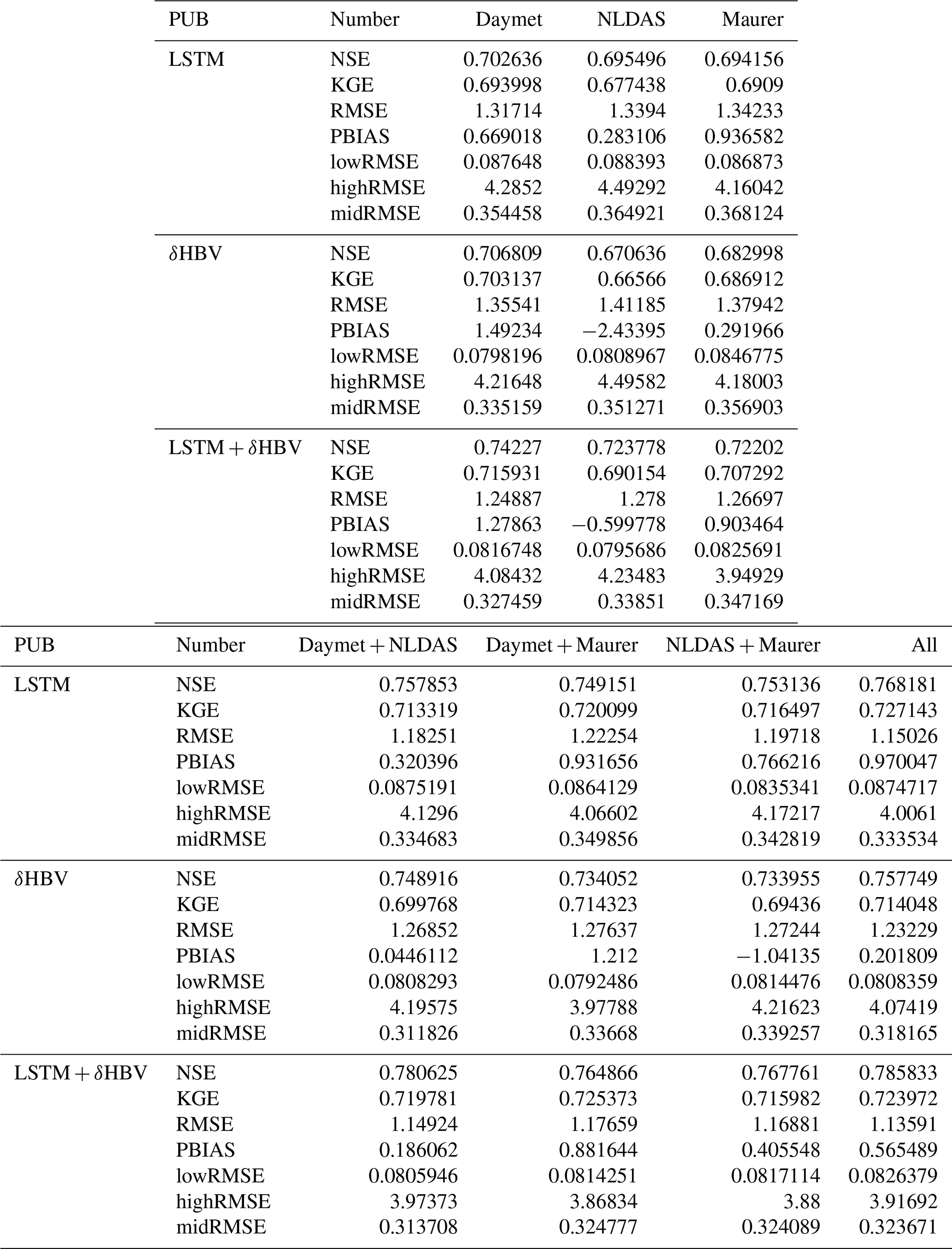
Table D3 Median NSE, KGE, RMSE, PBIAS, and RMSE values under low (lowRMSE), high (highRMSE), and middle (midRMSE) flows based on 531 basins under the PUR test. The values are the mean of three simulations run with different random seeds.

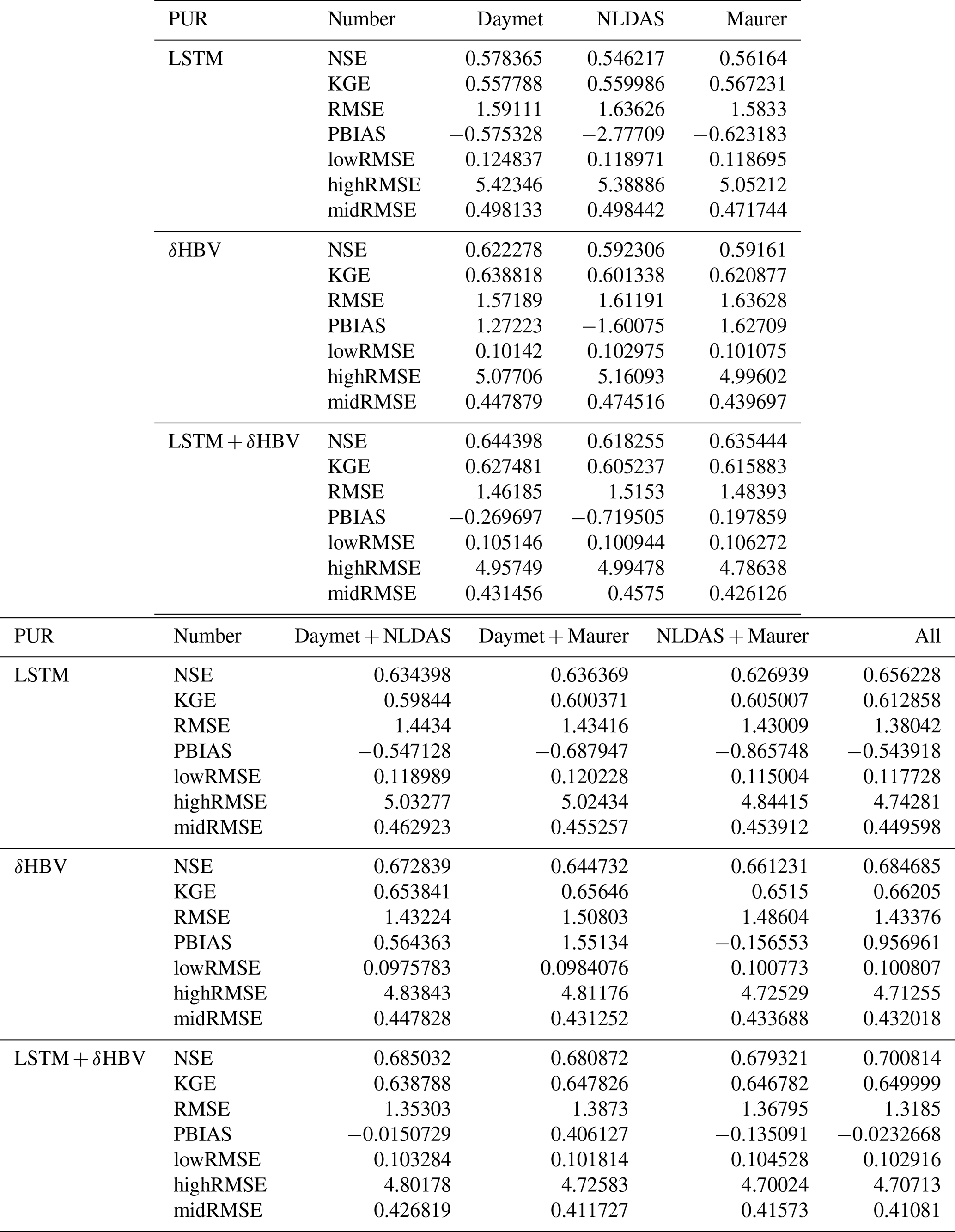
Table D4 Median NSE, KGE, RMSE, PBIAS, and RMSE values under low (lowRMSE), high (highRMSE), and middle (midRMSE) flows based on 531 basins under the temporal, PUB, and PUR tests of LSTM^multi, $(\mathrm{LSTM}+\mathit{\delta }\mathrm{HBV}{)}^{\mathrm{123}}+{\mathrm{LSTM}}^{\mathrm{multi}}$, their “seed” version, and $(\mathrm{LSTM}+\mathit{\delta }\mathrm{HBV}{)}_{\mathrm{seed}}^{\mathrm{123}}$.

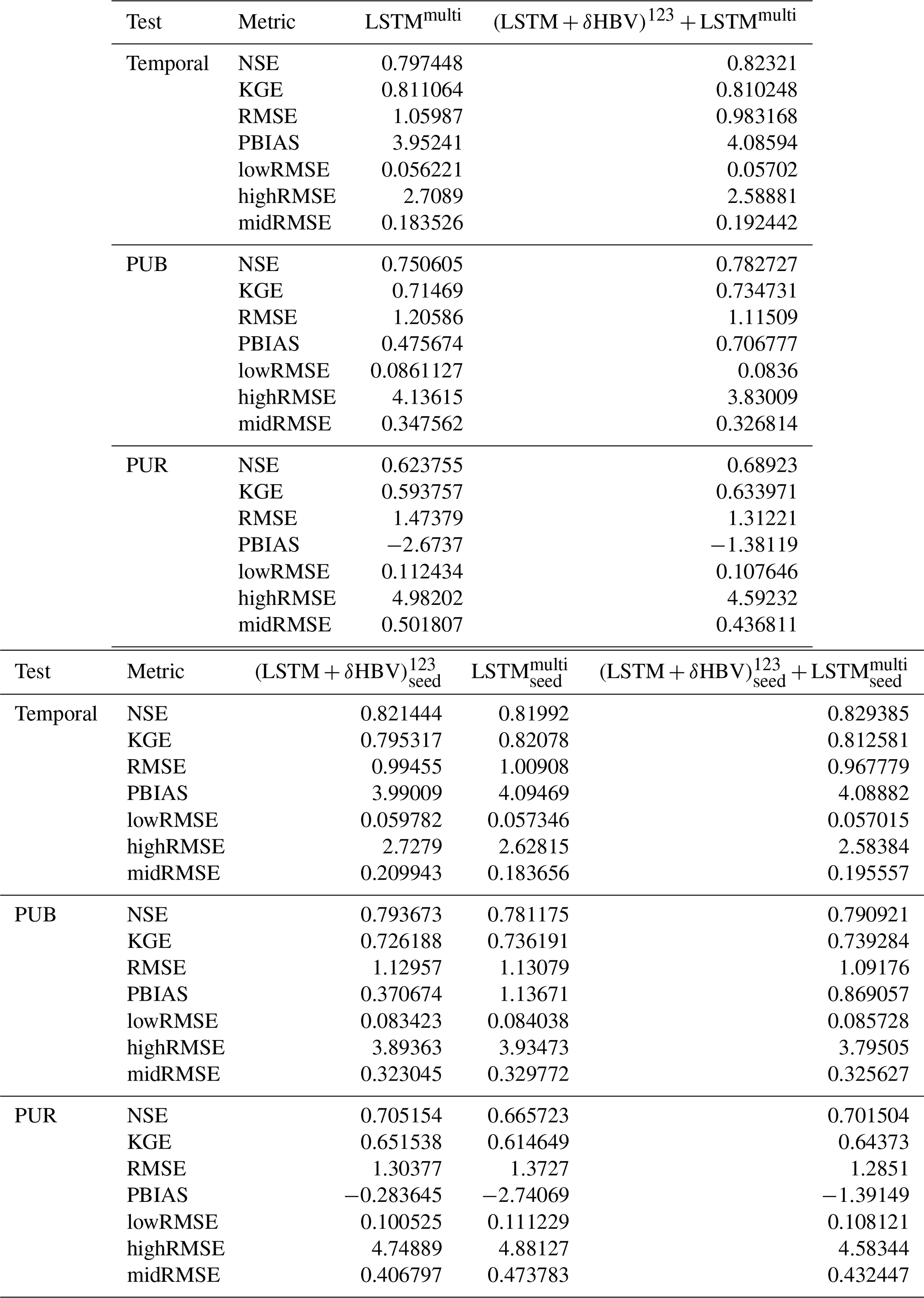
Table D5 Median NSE values based on ten different random seeds during the temporal test. Each number (1 through 10) represents metric values calculated for an individual simulation based on only one random seed. “Seed” indicates metric values calculated by averages of these ten simulations based on different random seeds, while “mean” denotes the average of metrics from 1–10 individual simulations (visualized in Fig. C1).

Appendix E: Intuitive visualization of the relative contributions of ensemble members based on optimized weights

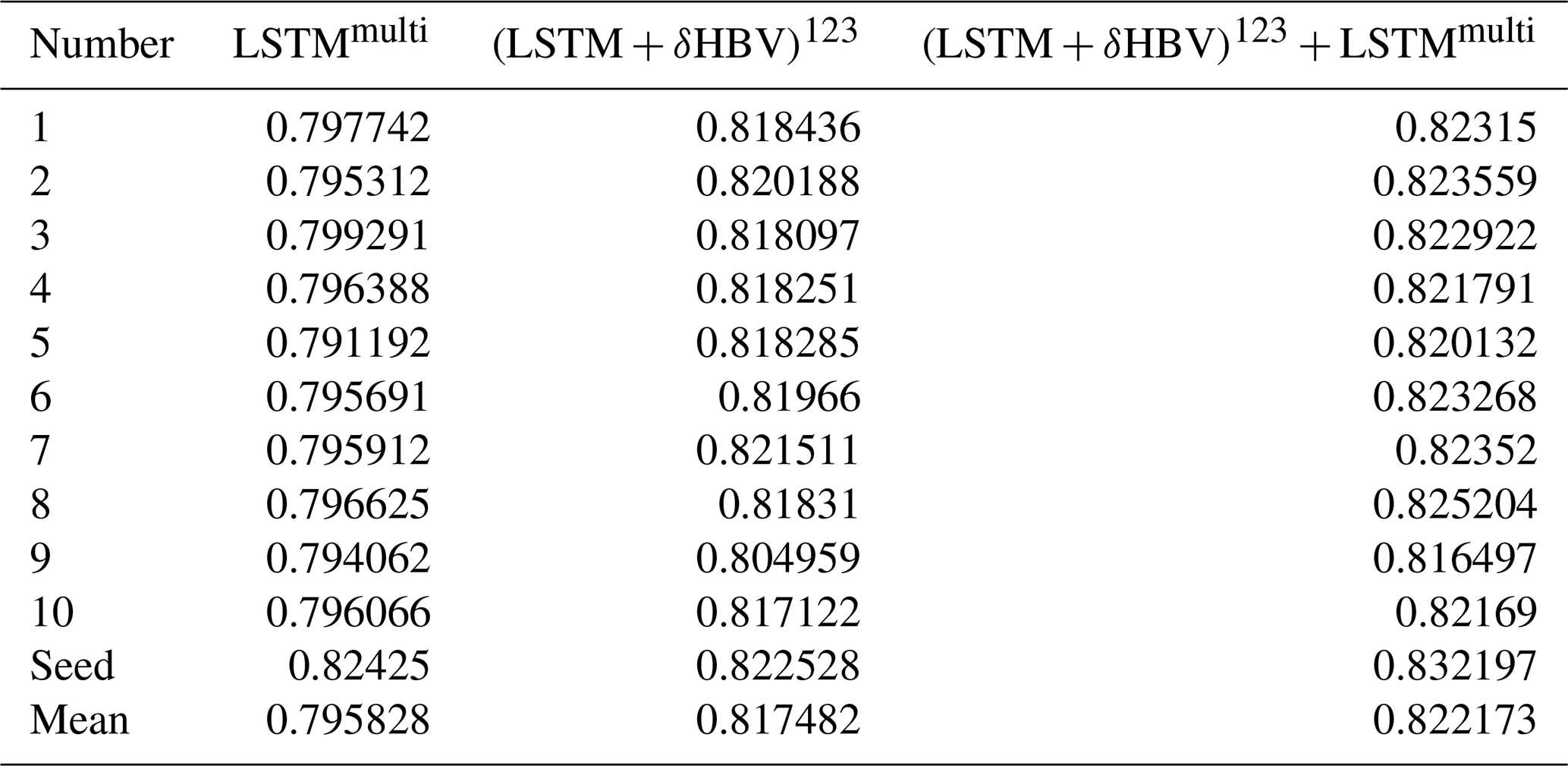
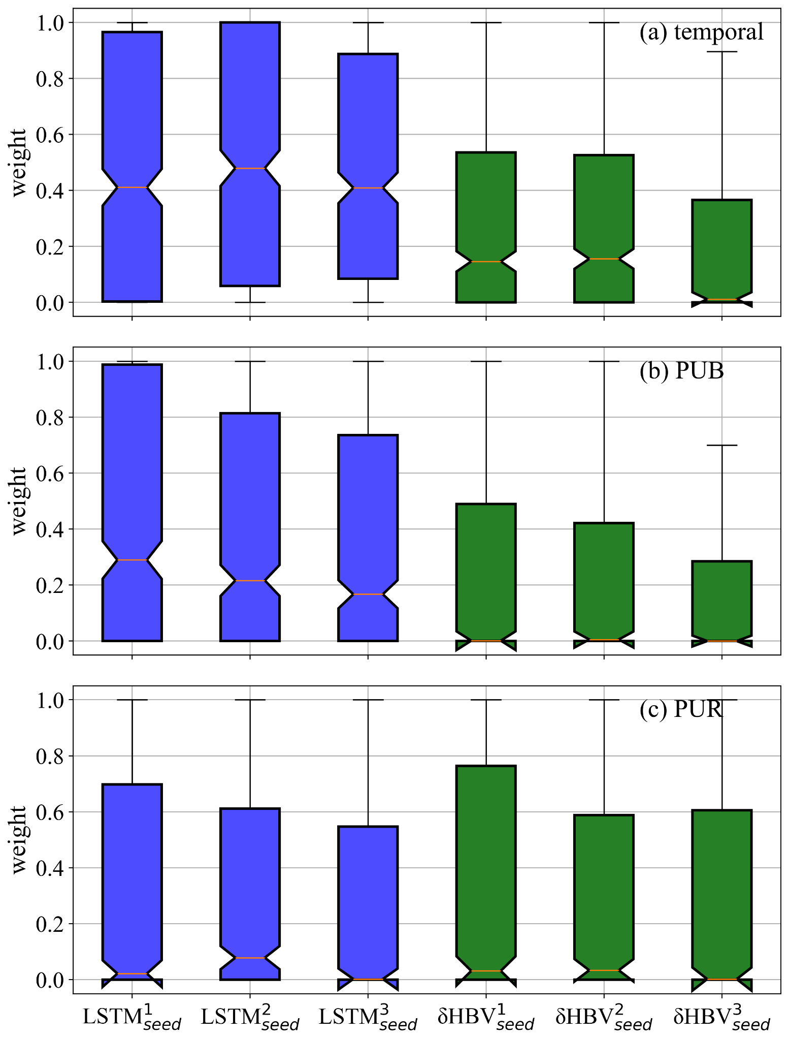
Figure E1 Weights of six components across 531 basins, estimated basin-by-basin using a genetic algorithm based on streamflow observations during the test periods. The weights are normalized by the maximum weight within each ensemble group. These weights are used exclusively for qualitatively analyzing the relative contributions of different ensemble members, with higher values indicating larger relative contributions.

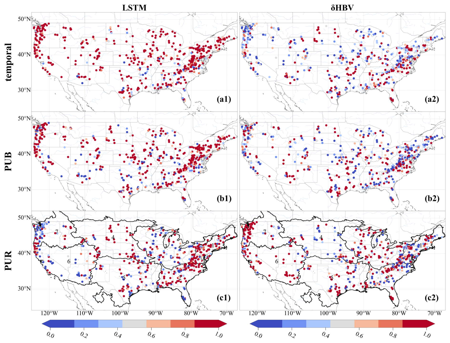
Figure E2 Spatial distributions of weights of the LSTM and δHBV models, estimated by a genetic algorithm based on streamflow observations during the test periods. The weights are normalized by the maximum weight within each ensemble group. These weights are used exclusively for qualitatively analyzing the relative contributions of different ensemble members, with higher values indicating larger relative contributions.

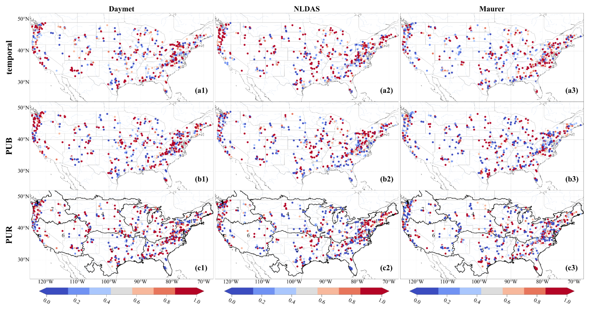
Figure E3 Spatial distributions of weights of the Daymet, NLDAS, and Maurer meteorological forcing datasets, estimated by a genetic algorithm based on streamflow observations during the test periods. The weights are normalized by the maximum weight within each ensemble group. These weights are used exclusively for qualitatively analyzing the relative contributions of different ensemble members, with higher values indicating larger relative contributions.

Table E1 Comparisons of metric values between averaged ensemble simulations and optimized weighted simulations, estimated using a genetic algorithm based on streamflow observations during the test periods. The results highlight the potential for further improvements in ensemble simulations.