Evaporation measurements using commercial microwave links as scintillometers

As the spatial coverage of evaporation observations is limited, we propose a novel, opportunistic method to estimate evaporation in which we consider commercial microwave links (CMLs), such as used in cellular telecommunication networks, in combination with scintillometry. Scintillometers are dedicated instruments to measure path-integrated latent and sensible heat fluxes, transmitting electromagnetic radiation that is diffracted by turbulent eddies between transmitter and receiver, causing the so-called scintillation effect. CMLs are line-of-sight devices that transmit electromagnetic radiation at similar frequencies as microwave scintillometers. However, CMLs and their sampling strategies are designed to ensure a continuously functioning wireless communication network rather than to capture the scintillation effect. Here, we estimate 30 min latent heat fluxes and daily evaporation using a former CML. To do so, we use data of a 38 GHz Nokia CML (formerly part of a telecom network) installed over an 856 m path at the Ruisdael Observatory near Cabauw, the Netherlands. We compare our results with estimates from an optical and microwave scintillometer setup, as well as an EC system. To obtain the flux estimates using the CML, we apply the two-wavelength method, in combination with the optical scintillometer, as well as a standalone energy-balance method (EBM), requiring net radiation estimates. For comparison, we also consider the free-convection limit of Monin-Obukhov similarity theory (MOST), instead of the complete scaling. An advantage of this approach is that it does not require horizontal wind speed measurements, which are more difficult to obtain in complex environments. For the net radiation estimates, we use in-situ measured radiation and data products provided by the Satellite Application Facility on Land Surface Analysis (LSA SAF) of EUMETSAT. Considering both turbulent heat fluxes, the two-wavelength method outperforms the EBM. The standalone EBM shows a reasonable performance, but also a large dependence on the quality of the net radiation estimates. When aggregating our 30 min latent heat fluxes to daily evaporation estimates, the relative performance of the methods remains comparable to that at 30 min intervals. These daily evaporation estimates could also be useful for catchment hydrological applications. Application of the free-convection scaling instead of the complete MOST scaling results in a comparable performance for all methods.

1 Introduction

Evaporation plays a key role in the energy and water cycle, yet large-scale evaporation observations are not readily available. Global coverage of in-situ networks, e.g., consisting of eddy-covariance (EC) systems, like FLUXNET, is relatively low and cannot represent all ecosystems and continents (e.g., Villarreal and Vargas, 2021; Pallandt et al., 2022). In comparison, satellite remote sensing estimates of evaporation have a better spatial coverage, but have a low temporal and limited spatial resolution (Zhang et al., 2016). Also, the method relies on indirect relations between surface characteristics and evaporation, while also clouds can be a limiting factor. As an alternative to these methods, Leijnse et al. (2007b) proposed using commercial microwave links (CMLs), which are near-surface terrestrial radio connections used in cellular telecommunication networks, as scintillometers to obtain latent and sensible heat flux estimates.

To measure evaporation, CMLs can be used in combination with scintillation theory, which derives turbulent characteristics of the atmosphere from fluctuations in the received signal intensity, so-called scintillations (e.g., Ward, 2017). The frequencies of the transmitted electromagnetic radiation by CMLs are comparable to those employed by microwave scintillometers, which are dedicated instruments to obtain the surface turbulent heat fluxes (e.g., Kohsiek, 1982; Green et al., 2001; Ward et al., 2015b). As the transmitted scintillometer signal propagates through the atmosphere, turbulent eddies scatter the beam, so that at the receiving end the signal intensity fluctuates. The scattering properties of the atmosphere, expressed as the structure parameter of the refractive index C_nn, depend on the frequency of the transmitted signal and density of these eddies, which is affected by temperature and humidity of these eddies. To separate the signal intensity fluctuations into temperature and humidity induced fluctuations, usually a two-wavelength scintillometer setup is used. This typically includes a microwave scintillometer (MWS), of which the signal is affected by both temperature and humidity fluctuations, and an optical scintillometer, of which the signal is mostly affected by temperature fluctuations. These separated fluctuations in temperature and humidity can be related to the surface turbulent heat fluxes using Monin-Obukhov similarity theory (Monin and Obukhov, 1954).

As an advantage, CML networks have a large spatial coverage, also at locations where in-situ observation networks are absent, and are actively maintained by mobile network operators. It is estimated that 6 million CMLs will be operationally employed in 2027 (ABI research, 2021). Moreover, CMLs are already used to measure path-averaged rainfall (e.g., Messer et al., 2006; Leijnse et al., 2007a), so that theoretically these networks could be used to measure both water fluxes between the atmosphere and land surface. However, using CMLs as scintillometers also introduces challenges, such as noise floors in antennas, power quantization (i.e., discretization of the signal intensity) and typical temporal sampling strategies in CML network management systems at relatively coarse temporal resolutions, i.e., ∼ 15 min (van der Valk et al., 2025a).

In this study, we build on the results of van der Valk et al. (2025a), where we aimed to obtain the best possible 30 min C_nn estimates using a CML formerly employed in a telecommunication network in the Netherlands. We found that the CML, an 38 GHz Nokia CML sampled at 20 Hz, adds white noise to the signal intensity, resulting in an overestimation of C_nn values. In order to correct for that, we proposed two methods. The first method applies a high-pass filter and subtracts a low quantile of the resulting variances of the Nokia CML, called the constant noise correction method. The second method corrects for the noise in the Nokia CML by comparing with an MWS and selecting parts of the power spectra where the Nokia Flexihopper behaves in correspondence with scintillation theory, called the spectral noise correction method. The latter method also considers different crosswind conditions and corrects for the omitted scintillations using scintillation theory. Both correction methods showed a major improvement in comparison to the uncorrected C_nn estimates. The spectral noise method outperformed the constant noise method, mostly by reducing the spread compared to the reference instruments, the MWS and an EC system. An advantage of the constant noise method is that it provides a straightforward correction, without the need for a collocated MWS. However, it is unclear what the effect of the uncertainty in these C_nn estimates on the eventual turbulent heat fluxes is. The aim of this study is to obtain latent heat fluxes using the proposed correction methods of van der Valk et al. (2025a).

Here, we focus on obtaining 30 min latent heat flux and daily evaporation estimates from the Nokia CML using the scintillometer method. To do so, we use the same Nokia CML as van der Valk et al. (2025a), which is installed at the Ruisdael Observatory near Cabauw, the Netherlands, and examine data between 1 April and 1 October 2024, corresponding to a full growing season in the Netherlands. We try to obtain flux estimates with the CML using the regular two-wavelength method, in which a microwave scintillometer is combined with an optical scintillometer. Moreover, we explore a standalone method based on the energy balance (as proposed by Leijnse et al., 2007b), which can be used to obtain the latent heat fluxes by combining the C_nn estimates with more widely available input data than an optical scintillometer. Additionally, to reduce the number of required meteorological observations, we consider the free-convection limit of Monin-Obukhov similarity theory, instead of the complete scaling. We elaborate on these methods in Sect. 2. We compare our latent heat flux estimates with a two-wavelength scintillometer setup (microwave and optical) and an EC setup. Overall, this setup allows us to investigate the potential of CMLs to estimate 30 min latent heat fluxes and daily evaporation in well-monitored and relatively idealized conditions.

2 Obtaining the turbulent heat fluxes from C_nn

To relate the structure parameter of the refractive index, C_nn, to the turbulent heat fluxes, first the structure parameters of temperature, C_TT, and humidity, C_qq, have to be determined. C_nn is affected by C_TT [K² m${}^{-\mathrm{2}/\mathrm{3}}$], C_qq [kg² kg⁻² m${}^{-\mathrm{2}/\mathrm{3}}$] and the cross-structure parameter C_Tq [K kg kg⁻¹ m${}^{-\mathrm{2}/\mathrm{3}}$] (e.g., Foken, 2021):

$$\begin{array}{}\text{(1)}& C_{nn}={\displaystyle \frac{A_T^{\mathrm{2}}}{{\stackrel{\mathrm{‾}}{T}}^{\mathrm{2}}}}{C}_{TT}+{\displaystyle \frac{A_q^{\mathrm{2}}}{{\stackrel{\mathrm{‾}}{q}}^{\mathrm{2}}}}{C}_{qq}+\mathrm{2}{\displaystyle \frac{A_T{A}_q}{\stackrel{\mathrm{‾}}{T}\stackrel{\mathrm{‾}}{q}}}{C}_{Tq},\end{array}$$

in which A_T and A_q are the structure parameter coefficients for temperature and specific humidity, respectively (e.g., given in Ward et al., 2013), $\stackrel{\mathrm{‾}}{T}$ is the average air temperature [K] and $\stackrel{\mathrm{‾}}{q}$ is the average specific humidity [kg kg⁻¹]. These coefficients are dependent on temperature, humidity, pressure and the wavelength of the scintillometer.

2.1 Two-wavelength setups

Typically in scintillometer systems, a two-wavelength setup is installed, so that C_TT and C_qq can be retrieved from the C_nn estimates of both scintillometers. Usually, this involves a microwave scintillometer (MWS) and a large-aperture scintillometer (LAS), which operates at optical wavelengths. The C_nn estimates obtained from the MWS are affected by both the temperature and humidity fluctuations in Eq. (1), while the C_nn estimates obtained from the LAS are dominated by temperature fluctuations. C_Tq can be measured by correlating the LAS and MWS signals (called bichromatic method; Lüdi et al., 2005) or estimated by assuming a value for the temperature-humidity correlation coefficient r_Tq:

$$\begin{array}{}\text{(2)}& C_{Tq}=r_{Tq}\sqrt{C_{TT}{C}_{qq}}.\end{array}$$

Typical values for r_Tq are around 0.8 for unstable conditions and −0.5 for stable conditions (Ward, 2017). Similar to Ward et al. (2015b), we assume r_Tq to be 0.8 for daytime conditions, who find this to be a reasonable value, consistent with values obtained from fast-response sensors (e.g., Kohsiek, 1982; Meijninger et al., 2002).

Subsequently, when using the two-wavelength method, C_TT and C_qq, can be computed using (e.g.,  Hill, 1997):

$$\begin{array}{}\text{(3)}& \begin{array}{rl}{C}_{TT}& ={\displaystyle \frac{A_{q\mathrm{2}}^{\mathrm{2}}{C}_{nn\mathrm{1}}+A_{q\mathrm{1}}^{\mathrm{2}}{C}_{nn\mathrm{2}}+\mathrm{2}{r}_{Tq}{A}_{q\mathrm{1}}{A}_{q\mathrm{2}}{S}_{\mathrm{2}\mathit{\lambda }}\sqrt{C_{nn\mathrm{1}}{C}_{nn\mathrm{2}}}}{(A_{T\mathrm{1}}{A}_{q\mathrm{2}}-A_{T\mathrm{2}}{A}_{q\mathrm{1}}{)}^{\mathrm{2}}{T}^{-\mathrm{2}}}},\\ C_{qq}& ={\displaystyle \frac{A_{T\mathrm{2}}^{\mathrm{2}}{C}_{nn\mathrm{1}}+A_{T\mathrm{1}}^{\mathrm{2}}{C}_{nn\mathrm{2}}+\mathrm{2}{r}_{Tq}{A}_{T\mathrm{1}}{A}_{T\mathrm{2}}{S}_{\mathrm{2}\mathit{\lambda }}\sqrt{C_{nn\mathrm{1}}{C}_{nn\mathrm{2}}}}{(A_{T\mathrm{1}}{A}_{q\mathrm{2}}-A_{T\mathrm{2}}{A}_{q\mathrm{1}}{)}^{\mathrm{2}}{q}^{-\mathrm{2}}}},\end{array}\end{array}$$

in which subscripts 1 and 2 refer to the LAS and MWS, respectively, and S_2λ originates from the two possible solutions for the C_nn of microwave signals (Hill, 1997). When humidity fluctuations dominate (i.e., a low Bowen ratio) S_2λ equals 1, while when temperature fluctuations dominate (i.e., a high Bowen ratio) S_2λ equals −1. For our study, we assume S_2λ equals 1, given the relatively wet conditions at our field site (e.g., Brauer et al., 2014).

After obtaining C_TT and C_qq, these can be related to the turbulent heat fluxes using Monin-Obukhov similarity theory (MOST). First, C_TT and C_qq are related to the average turbulent temperature ${\stackrel{\mathrm{‾}}{T}}_{*}$ [K] and humidity scales ${\stackrel{\mathrm{‾}}{q}}_{*}$ [kg kg⁻¹],

$$\begin{array}{}\text{(4)}& \begin{array}{rl}& {\displaystyle \frac{C_{TT}{z}^{\mathrm{2}/\mathrm{3}}}{{\stackrel{\mathrm{‾}}{T}}_{*}^{\mathrm{2}}}}=f_{TT}\left({\displaystyle \frac{z-d}{L_{\mathrm{Ob}}}}\right),\\ & {\displaystyle \frac{C_{\mathrm{qq}}{z}^{\mathrm{2}/\mathrm{3}}}{{\stackrel{\mathrm{‾}}{q}}_{*}^{\mathrm{2}}}}=f_{qq}\left({\displaystyle \frac{z-d}{L_{\mathrm{Ob}}}}\right),\end{array}\end{array}$$

in which z is the measurement height [m], d is the displacement height [m], L_Ob is the Obukhov length [m], and f_TT and f_qq are universal functions (e.g., Wyngaard et al., 1971b). The turbulent heat fluxes are directly related to T_* and q_*:

$$\begin{array}{}\text{(5)}& \begin{array}{rl}& T_{*}=-{\displaystyle \frac{H}{\stackrel{\mathrm{‾}}{\mathit{\rho }}{c}_{\mathrm{p}}{u}_{*}}},\\ & q_{*}={\displaystyle \frac{(\mathrm{1}-\stackrel{\mathrm{‾}}{q})L_{\mathrm{v}}E}{\stackrel{\mathrm{‾}}{\mathit{\rho }}{L}_{\mathrm{v}}{u}_{*}}},\end{array}\end{array}$$

in which H is the sensible heat flux [W m⁻²], L_vE is the latent heat flux [W m⁻²], ρ is the air density [kg m⁻³], c_p is the specific heat capacity of air [J kg⁻¹ K⁻¹], u_* is the friction velocity [m s⁻¹] and L_v is the latent heat of vaporization [J kg⁻¹].

The f_TT and f_qq functions usually have the form (for unstable conditions):

$$\begin{array}{}\text{(6)}& f\left({\displaystyle \frac{z-d}{L_{\mathrm{Ob}}}}\right)=c_{\mathrm{1}}{\left(\mathrm{1}-c_{\mathrm{2}}\left({\displaystyle \frac{z-d}{L_{\mathrm{Ob}}}}\right)\right)}^{-\mathrm{2}/\mathrm{3}},\end{array}$$

in which c₁ and c₂ are constants that differ for f_TT and f_qq and depend on stability. Kooijmans and Hartogensis (2016) compare measurements from different datasets in order to obtain robust similarity functions including an uncertainty range for these functions. For f_TT in unstable conditions, c₁ and c₂ are equal to 5.6 and 6.5, respectively. For f_qq in unstable conditions, c₁ and c₂ are equal to 4.5 and 7.3, respectively. L_Ob is defined as:

$$\begin{array}{}\text{(7)}& L_{\mathrm{Ob}}=-{\displaystyle \frac{\stackrel{\mathrm{‾}}{\mathit{\rho }}{c}_{\mathrm{p}}\stackrel{\mathrm{‾}}{T}{u}_{*}^{\mathrm{3}}}{g\mathit{\kappa }H}},\end{array}$$

in which g is the gravitational acceleration [m s⁻²] and κ is the von-Karmán constant. u_* can be calculated using horizontal wind speed measurements U [m s⁻¹]:

$$\begin{array}{}\text{(8)}& u_{*}={\displaystyle \frac{\mathit{\kappa }U}{\log \left(\frac{z_u-d}{z_{\mathrm{0}}}\right)-{\mathit{\psi }}_M\left(\frac{z_u-d}{L_{\mathrm{Ob}}}\right)+{\mathit{\psi }}_M\left(\frac{z_{\mathrm{0}}}{L_{\mathrm{Ob}}}\right)}},\end{array}$$

in which z_u is the measurement height of U [m], z₀ is the roughness length for momentum [m] and ψ_M is the Businger-Dyer expression (e.g., Brutsaert, 1982).

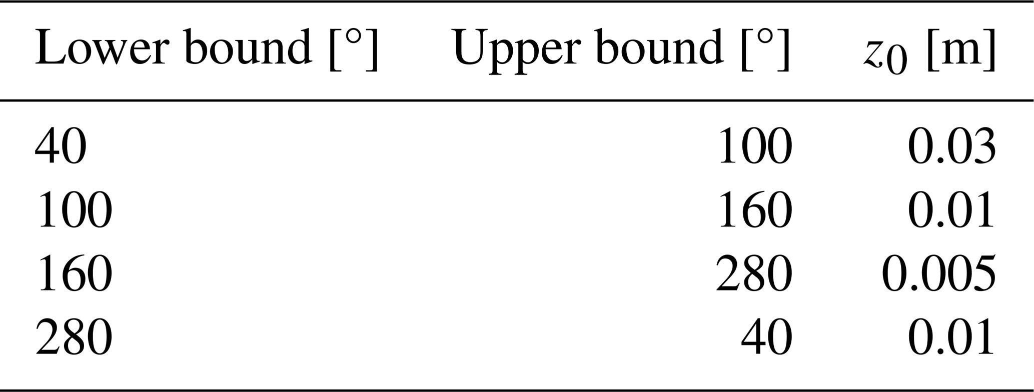
Thus, next to the scintillometer measurements, the two-wavelength method requires temperature, humidity and horizontal wind speed measurements. Additionally, it requires more complex measurements of the correlation between temperature and humidity fluctuations, the roughness length for momentum and the displacement height. For the roughness length z₀, we make use of values reported by Moonen (2021), who determined the roughness length for various wind sectors using EC data (Table 1) and found similar values to Verkaik and Holtslag (2007). For the displacement height d, we use the relationship $d=\frac{\mathrm{16}}{\mathrm{3}}{z}_{\mathrm{0}}$ from Brutsaert (1982).

In order to obtain the turbulent heat fluxes, Eqs. (4)–(7) have to be solved iteratively. In figures, we refer to the two-wavelength method using the suffix 2λ. We refer the reader to Appendix A for a complete overview of the used abbreviations.

Table 1 Lower and upper bound of wind direction classes and roughness length z₀ values as determined by Moonen (2021).

2.2 Standalone methods

To compute the turbulent heat fluxes using CMLs, a LAS is usually not available, so that standalone methods need to be defined. These standalone methods require an additional constraint or assumption in order to separate C_nn into C_TT and C_qq, and subsequently into the turbulent heat fluxes. In this study, we use the energy balance as constraint, hereafter referred to as EBM (Leijnse et al., 2007b). To do so, closure of the measured energy balance is assumed:

$$\begin{array}{}\text{(9)}& R_{\mathrm{net}}-G=L_{\mathrm{v}}E+H,\end{array}$$

in which R_net is the net radiation [W m⁻²] and G is the ground heat flux [W m⁻²]. In combination with Eqs. (1), (4)–(8), both the turbulent heat fluxes can be solved iteratively. In this study, we apply this method using in-situ measurements and LSA SAF data products to obtain the net radiation (Sect. 3.3). For the in-situ method, we use the measured ground heat flux, while for the remotely sensed data product we assume 10 % of the net radiation is used for the ground heat flux. Note that the measured energy balance hardly ever closes, especially in more complex measurement environments, e.g., forests or cities (Mauder et al., 2020). For the field site used in this study, Cabauw in the Netherlands, typically an imbalance during day-time is found between 10 % (afternoons) to 40 % (mornings) (Kroon, 2004). For our data period we find similar values using EC data (not shown).

As alternative constraint, we considered prescribing a Bowen ratio instead of net radiation, however that did not yield promising results. We applied the Bowen ratio obtained from the estimated turbulent heat fluxes by LSA SAF. An advantage is that this does not require radiation estimates, but the performance depends largely on the quality of the prescribed Bowen ratio. In the remainder of this article, we refer to the EBM using in-situ radiation data with EBM-OBS, and for the method using the LSA data products, we use EBM-LSA. We refer the reader to Appendix A for a complete overview of the used abbreviations.

2.3 Free-convection scaling

Free-convection scaling can be applied to further reduce the number of required meteorological observations, as no horizontal wind speed measurements are necessary. This scaling assumes the turbulent heat fluxes are solely a result of convection. A disadvantage of this assumption is that it introduces an underestimation of the turbulent heat fluxes in comparison to the complete scaling, which also includes wind shear as source of the fluxes. However, this underestimation is relatively little as, using the method of De Bruin et al. (1995) to estimate the underestimation of free-convection, we find that L_vE is underestimated less than 5 % for $-\frac{z-d}{L_{\mathrm{Ob}}}$ values larger than 1 (Fig. 1). An advantage of CMLs is that they are typically mounted relatively high above the ground surface (at least 20–30 m), especially in comparison to typical scintillometer heights, so that $-\frac{z-d}{L_{\mathrm{Ob}}}$ also is relatively large with constant L_Ob.

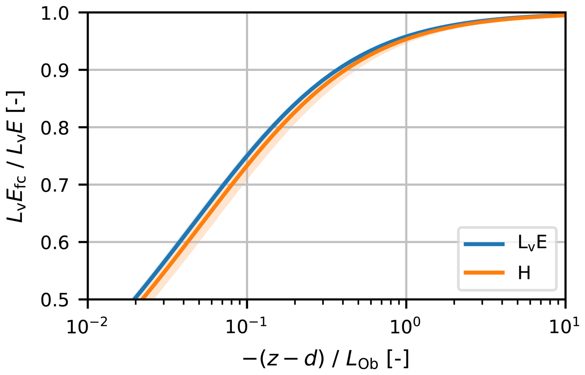
Figure 1 Underestimation of the free-convection scaling versus the complete scaling as function of $-\frac{z-d}{L_{\mathrm{Ob}}}$. The bands indicate the uncertainty based on the uncertainty estimates of the MOST universal functions coefficients by Kooijmans and Hartogensis (2016). For L_vE this uncertainty band is relatively small in comparison to H.

For free-convection scaling, C_TT and C_qq in Eq. (4) are not scaled with T_* and q_*, but with T_fc and q_fc, which are defined as (Wyngaard et al., 1971a):

$$\begin{array}{}\text{(10)}& \begin{array}{rl}{T}_{\mathrm{fc}}& ={\displaystyle \frac{H}{\stackrel{\mathrm{‾}}{\mathit{\rho }}{c}_p{u}_{\mathrm{fc}}}},\\ q_{\mathrm{fc}}& ={\displaystyle \frac{L_{\mathrm{v}}E}{\stackrel{\mathrm{‾}}{\mathit{\rho }}{L}_{\mathrm{v}}{u}_{\mathrm{fc}}}},\end{array}\end{array}$$

in which u_fc is the scaling wind velocity [m s⁻¹], defined as:

$$\begin{array}{}\text{(11)}& u_{\mathrm{fc}}={\left({\displaystyle \frac{g(z-d)}{T}}{\displaystyle \frac{H}{\mathit{\rho }{c}_p}}\right)}^{\mathrm{1}/\mathrm{3}}.\end{array}$$

Finally, replacing T_* and q_* in Eq. (4) with T_fc and q_fc and assuming $-\left(\frac{z}{L_{\mathrm{Ob}}}\right)$ goes to infinity, results in Kohsiek (1982):

$$\begin{array}{}\text{(12)}& \begin{array}{rl}H& =\pm a\mathit{\rho }{c}_{\mathrm{p}}(z-d){\left({\displaystyle \frac{g}{T}}\right)}^{\mathrm{1}/\mathrm{2}}{C}_{TT}^{\mathrm{3}/\mathrm{4}},\\ L_{\mathrm{v}}E& =\pm b\mathit{\rho }{L}_{\mathrm{v}}(z-d){\left({\displaystyle \frac{g}{T}}\right)}^{\mathrm{1}/\mathrm{2}}{C}_{TT}^{\mathrm{1}/\mathrm{4}}{C}_{qq}^{\mathrm{1}/\mathrm{2}},\end{array}\end{array}$$

in which a and b are empirical constants based on the universal function (Eq. 6), which are 0.44 and 0.51 respectively, using the values reported by Kooijmans and Hartogensis (2016). Using their reported uncertainty of these coefficients, a ranges between 0.37 and 0.51, and b between 0.47 and 0.56. In Sect. 4, we apply the complete and free-convection scaling for all our methods, and refer to the latter in the figures with suffix FC. We refer the reader to Appendix A for a complete overview of the used abbreviations.

3 Instrument and data description

3.1 Experimental setup

We use the same experimental setup as van der Valk et al. (2025a). This experiment is conducted at the Ruisdael Observatory at Cabauw, the Netherlands. We installed a commercial microwave links collocated to a MWS and LAS setup over an 856 m path between 51.974252° N, 4.923484° E and 51.967552° N, 4.929561° E (Fig. 2). The CML and scintillometers are installed on a 10 m high, vibration-free mast. We use daytime data from from 1 April to 1 October 2024, which corresponds to a growing season in the Netherlands. Moreover, it is important to note that management of the water table aims to have a constant soil water content in the rootzone, approximately at field capacity (e.g., Brauer et al., 2014). The dominant wind direction at Cabauw is southwesterly, so that the footprints of the scintillometers and EC mostly consist of grass fields. Only for northerly wind directions built-up area may partly be included.

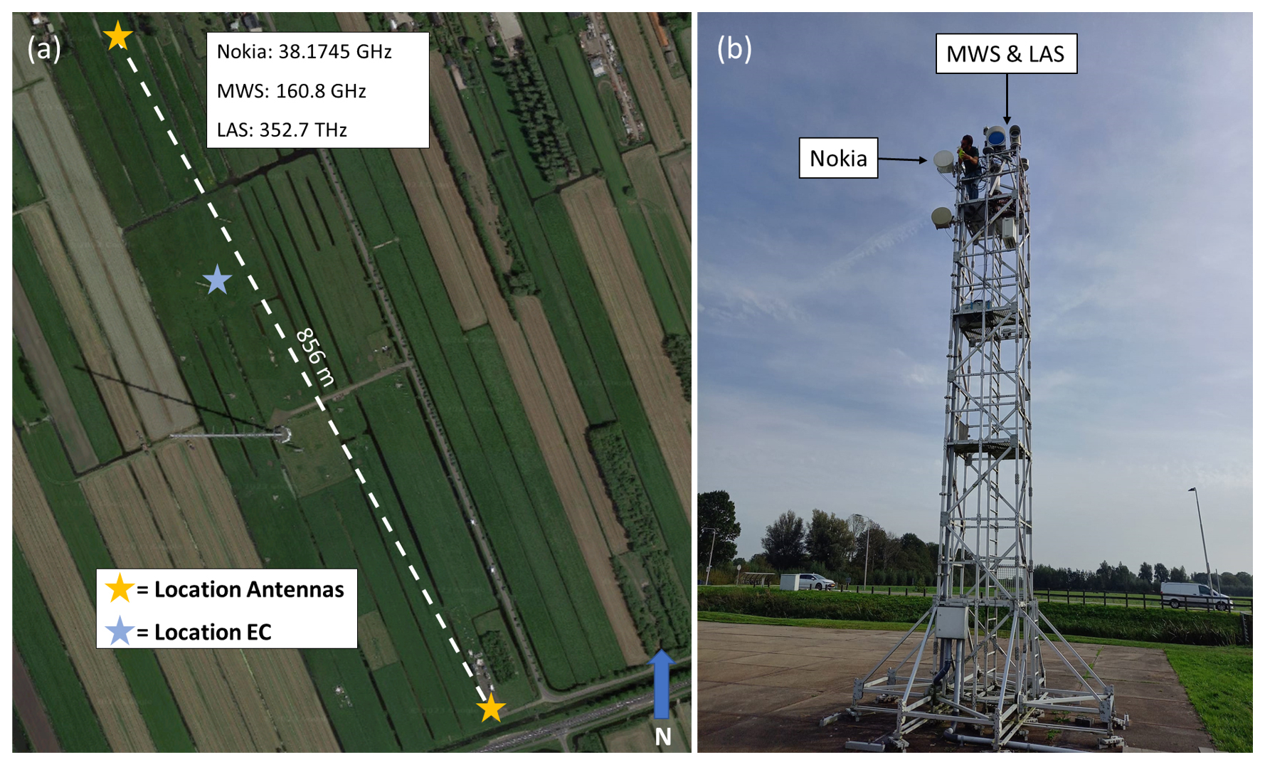
Figure 2 (a) Overview of (formerly employed) Nokia CML, MWS, LAS and EC at the Ruisdael Observatory, Cabauw. Reported frequencies are the transmitting frequencies per antenna. (b) The southern mast with 3 installed instruments. From top to bottom: the receivers of the MWS and LAS, the Nokia Flexihopper and an Ericsson MiniLink (not used in this study). Figure is based on van der Valk et al. (2025a) (© Google Maps).

3.2 Measurement equipment

The CML used in this study is a Nokia Flexihopper, formerly employed in a commercial mobile phone network operated by T-Mobile Netherlands (currently, Odido Netherlands). This link is mounted at 10 m above the surface and transmits at 38.1745 GHz with a bandwidth of 0.9 MHz. The signal intensity is sampled at 20 Hz. In van der Valk et al. (2025a), it is shown that the signal of this CML contains added white noise. Therefore, we suggest two C_nn correction methods, a constant noise correction method, which is a more generic correction, and a spectral noise correction method. Even though the constant noise method is outperformed by the spectral noise method, we show results of both methods in our current analysis, because the constant noise method is a straightforward correction method, which can be applied without a comparison with an MWS.

As reference instruments, we use an optical-microwave scintillometer setup and an eddy-covariance system (EC). The scintillometer setup consists of a Radiometer Physics RPG-MWSC-160 microwave scintillometer, transmitting at 160.8 GHz (i.e., a wavelength of 1.86 mm), and a Kipp & Zonen LAS Mk-II, transmitting at 352.7 THz (i.e., a wavelength of 850 nm), which are both sampled at 1 kHz. Hereafter we refer to this system as MWS-2λ. The path of this scintillometer setup is nearly identical to the path of the CML (e.g., Fig. 2), so that differences in footprints can be neglected. It should be noted that this setup has a major data gap between 10 July and 6 September 2024. The EC system consists of a sonic anemometer (Gill-R50) and an open-path H₂O $/$ CO₂ sensor (LICOR-7500), sampled at 10 Hz, and installed at 3 m above the ground (Bosveld et al., 2020). The fluxes obtained with the EC can directly obtained from the KNMI Data Platform (2024), next to other more common meteorological measurements. The EC data is available during the entire study period. During the dominant south-westerly wind direction, the footprints of the EC, scintillometer setup and CML all predominantly consist of grass fields.

After computing 30 min L_vE estimates, we perform our analysis based on 30 min L_vE [W m⁻²] and daily E [mm d⁻¹] estimates. The former is a typical time interval for turbulent heat flux research (e.g., Green et al., 2001; Meijninger et al., 2002), while the latter time scales are more commonly used in hydrological applications. In order to be able to compare daily E estimates, we only aggregate the 30 min time intervals per day that are available for both the Nokia CML and the reference instrument.

In our analysis, we remove nighttime intervals and intervals with high absolute wind speeds. We assume incoming shortwave radiation above 20 W m⁻² to exclude nighttime intervals, during which negligible evaporation takes place. As threshold for absolute wind speeds we use 8 m s⁻¹, because the Nokia CML vibrates during higher wind speeds (van der Valk et al., 2025a). This is caused by the relatively weak mounting system of the Nokia, as no vibrations are found in MWS even though both are mounted in the same mast. Additionally, we remove rainy intervals or those following a rain event within an hour, in order to exclude the effects of wet-antenna attenuation.

3.3 Remotely-sensed net radiation estimates

For the method of Leijnse et al. (2007b), net radiation measurements are required. To overcome the lacking availability of these measurements for CML networks, we consider the radiation products of Satellite Application Facility on Land Surface Analysis (LSA SAF) of EUMETSAT (EUMETSAT, 2025). Similar to Rains et al. (2024), we use the 15 min incoming shortwave radiation SW_↓ [W m⁻²], 30 min incoming longwave radiation LW_↓ [W m⁻²], daily albedo α, daily emissivity ϵ and 30 min land surface temperature T_surf [K] products to compute 30 min net radiation estimates using:

$$\begin{array}{}\text{(13)}& R_{\mathrm{net}}={\mathrm{SW}}_{\downarrow }+{\mathrm{LW}}_{\downarrow }-\mathit{\alpha }{\mathrm{SW}}_{\downarrow }-(\mathit{ϵ}\mathit{\sigma }{T}_{\mathrm{surf}}^{\mathrm{4}}+(\mathrm{1}-\mathit{ϵ}\left){\mathrm{LW}}_{\downarrow }\right),\end{array}$$

in which σ is the Stefan-Boltzmann constant (i.e., 5.67 × 10⁻⁸ W m⁻² K⁻⁴). In order to obtain 30 min net radiation estimates, we average SW_↓ to 30 min time intervals and assume α and ϵ are constant for the full day. Note that $(\mathrm{1}-\mathit{ϵ}){\mathrm{LW}}_{\downarrow }$ in the outgoing longwave radiation term originates from long-wave reflection (e.g., Maes and Steppe, 2012). Rains et al. (2024) show that hourly net radiation obtained with LSA SAF performs generally comparable to other large-scale products, e.g., the ERA5-Land product, and has on average a root mean square error of 23.5 W m⁻², an average bias of −9 W m⁻² and a correlation coefficient of 0.93 when comparing to in-situ data over Europe. For Cabauw during our data period, the net radiation obtained with LSA SAF compared to the measured net radiation on average shows similar error estimates, though with an overestimation (Fig. B1).

3.4 Error estimates

In this study, we compare 30 min L_vE estimates and daily E estimates [mm d⁻¹]. In all comparisons, we use the mean bias error (MBE), the 10–90 interquantile range (IQR) and Pearson's correlation coefficient (r). The MBE and IQR are calculated as:

$$\begin{array}{}\text{(14)}& \begin{array}{rl}\text{MBE}& =\stackrel{\mathrm{‾}}{y-x},\\ \text{IQR}& =P_{\mathrm{90}}-P_{\mathrm{10}},\end{array}\end{array}$$

in which y are the L_vE or E estimates of the instrument on the y-axis and x are the L_vE and E estimates of the instrument on the x-axis, i.e., the reference MWS-2λ or EC system. Similarly, P₉₀ and P₁₀ are the 90th and 10th percentiles of the difference between the L_vE or E estimates of the instrument on the y-axis and the L_vE or E estimates of the instrument on the x-axis of a scatterplot. The units of the MBE and IQR are the same as the variable presented in the scatterplot.

4 Results

4.1 30 min L_vE estimates

A comparison of the reference methods for the full data period shows an overall comparable behaviour (Fig. 3), indicating negligible influence of differences in footprints between the two references. On average, however, the MWS-2λ method shows an overestimation in comparison to EC. For the monthly median diurnal cycles, all CML methods with the spectral noise correction overestimate L_vE compared to the references (Fig. 4). This overestimation is roughly constant throughout our data period, with the exception of June, during which the overestimation in comparison to the reference methods is larger. The diurnal cycle is well captured by all CML methods, even when considering the interquartile range. Noteworthy, is the similarity between the CML-2λ and CML-EBM-OBS methods in the diurnal cycles, both in median values and uncertainty. The clearest differences between these methods occur before sunset, when the CML-2λ method overestimates LvE, while the CML-EBM-OBS estimates are constrained by the measured net radiation.

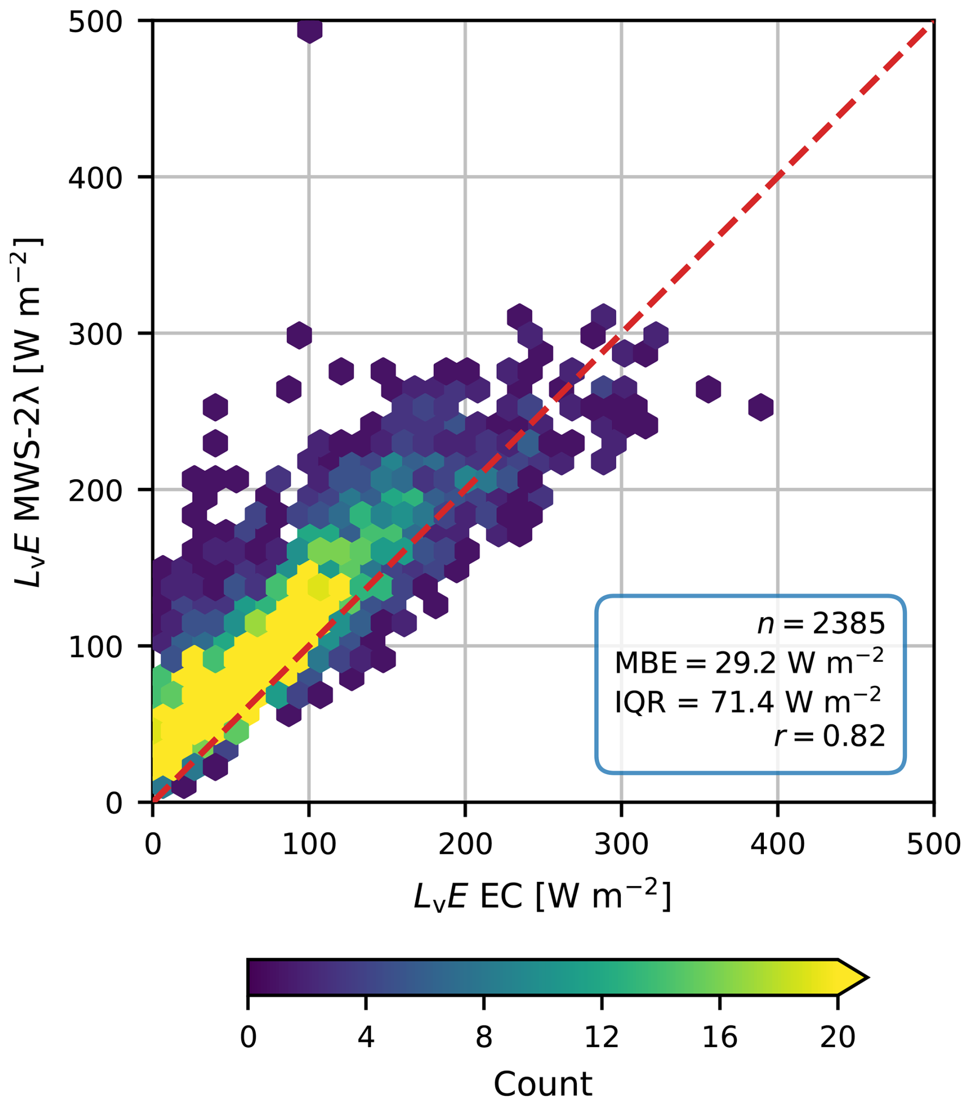
Figure 3 Comparison of 30 min L_vE estimates obtained with the MWS-2λ method versus the EC estimates. MWS-2λ method uses the 2 wavelength scintillation method with the MWS and LAS, and EC are the eddy-covariance estimates. The dashed red line is the 1:1 line.

Subsequently, we examine the performance of both corrections (constant and spectral noise), all methods (two-wavelength, EBM-OBS and EBM-LSA) and both scalings (complete and free-convection) in comparison to our reference instruments. Figure 5 shows scatter density plots for both correction methods with the two-wavelength method using the complete scaling. These plots show that the two example time series are not fully representative of the overall performance. For example, the typically found overestimation of high L_vE values for CML-2λ are not visible in Fig. 4b. In Fig. 6, we present all statistical metrics for the 30 min L_vE estimates using all possible combinations of corrections, methods and scalings. In this plot, we also show the intercomparison between the reference methods and two comparisons with alternative methods to derive L_vE. These alternatives are the L_vE estimates obtained directly from LSA SAF versus those from the MWS-2λ method and L_vE estimates based on R_net−G and a Bowen ratio versus those from the MWS-2λ method. We show these methods to illustrate how a readily available (former) and a basic experimental method from only net radiation estimates (latter) perform in comparison to the reference instruments. The used Bowen ratio is obtained from the EC and is the median ratio for the full data period (excluding nighttime intervals). We use a median value as a means to obtain an objectively selected, representative Bowen ration value to estimate L_vE from only net radiation measurements. For all the corresponding scatter density plots we refer the reader to the supplementary materials. The statistical plot for H can be found in Appendix C, and the corresponding scatter density plots can also be found in the Supplement.

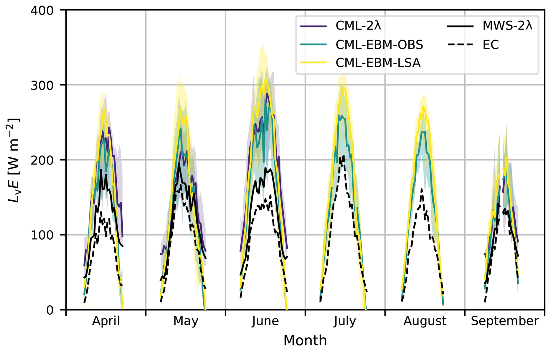
Figure 4 Median diurnal cycles and interquartile ranges (shading) of 30 min L_vE estimates of the methods for the Nokia CML in comparison with the reference instruments. CML-2λ method uses the two-wavelength scintillation method with the CML and LAS, CML-EBM-OBS uses the measured energy balance method as constraint to infer the turbulent heat fluxes and CML-EBM-LSA uses the estimated net radiation by LSA SAF instead of the measured net radiation. Shown estimates are obtained using the spectral noise method for the CML estimates and complete Monin-Obukhov scaling. We removed timestamps with less than 10 available days in order to obtain representative diurnal cycles. We refer the reader to Appendix A for a complete overview of the used abbreviations.

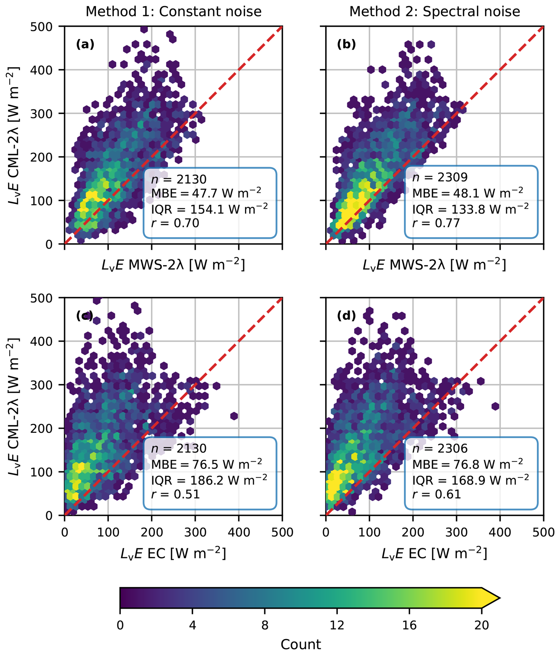
Figure 5 Comparison of 30 min L_vE estimates obtained with the Nokia CML using the two-wavelength method with the complete scaling for the entire study period, post-processed with the constant noise method (a, c) and spectral noise method (b, d) versus the MWS-2λ method (a, b) and the EC (c, d) estimates. The dashed red line is the 1:1 line.

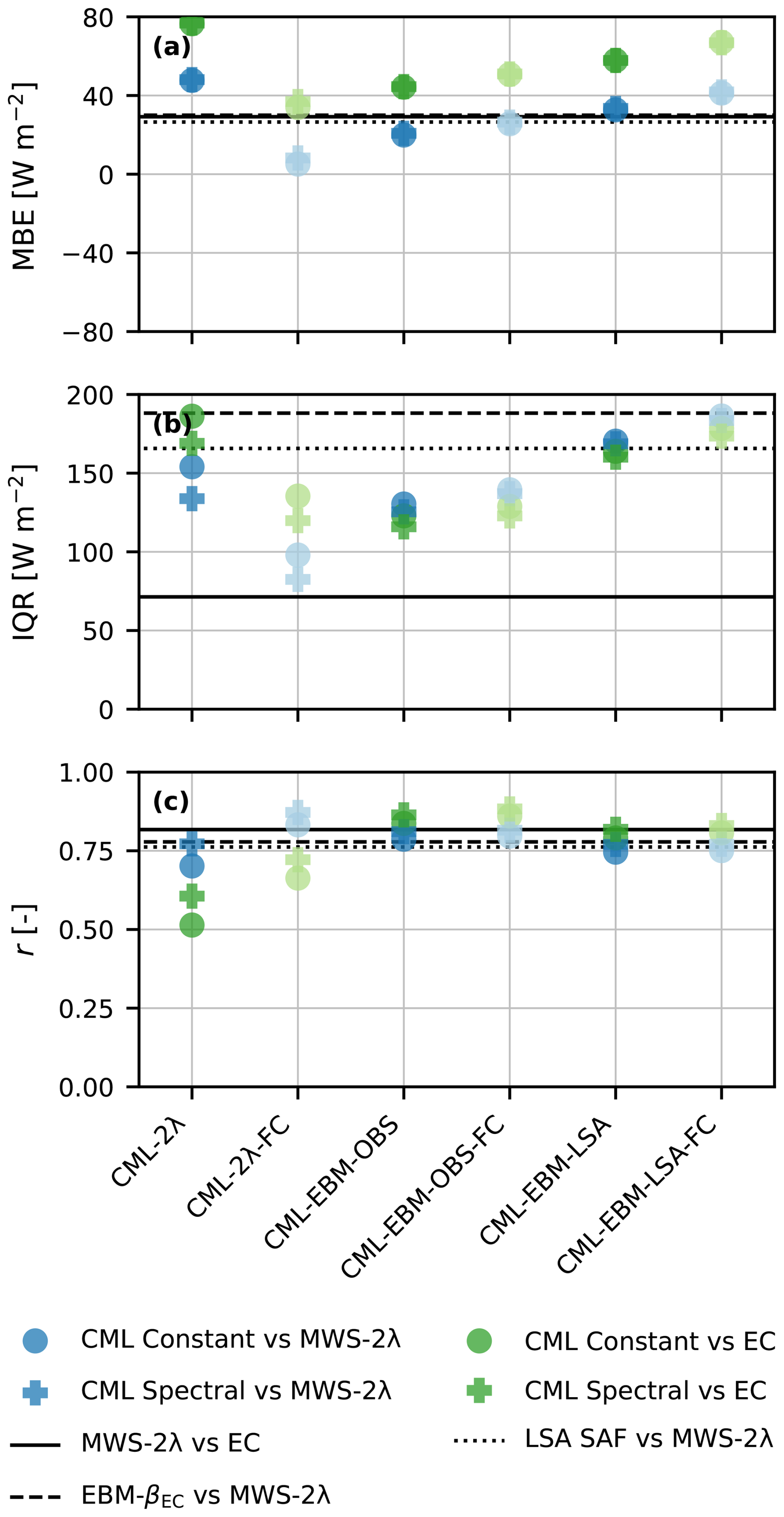
Figure 6 Statistical metrics per method and scaling to obtain L_vE estimates using the Nokia CML for both correction methods (shape) versus both reference instruments (color). The solid line indicates the statistical metrics of the reference instruments versus each other (Fig. 3). CML-2λ method uses the two-wavelength scintillation method with the CML and LAS, CML-EBM-OBS uses the measured energy balance method as constraint to infer the turbulent heat fluxes and CML-EBM-LSA uses the estimated net radiation by LSA SAF instead of the measured net radiation. The “FC”-suffix refers to the free-convection scaling. The dotted line shows the statistical metrics of a comparison between the L_vE estimates directly obtained from LSA SAF versus the MWS-2λ method. The dashed line represents L_vE estimates based on the measured available energy (R_net−G) and the Bowen ratio β obtained from the EC-system, i.e., $\frac{R_{\mathrm{net}}-G}{\mathrm{1}+\mathit{\beta }}$ versus the MWS-2λ method. The used Bowen ratio is a median value for the full data period (excluding nighttime intervals), as a means to obtain an objectively selected, representative Bowen ratio value to estimate L_vE from only net radiation measurements. We refer the reader to Appendix A for a complete overview of the used abbreviations.

4.1.1 Energy-balance method versus two-wavelength method

Overall, the EBM-OBS outperforms the other two methods for the L_vE estimates. It has a lower MBE and IQR than the two-wavelength method and the EBM-LSA. All methods have a comparable r in comparison to the MWS-2λ method. We would have expected the two-wavelength method to perform best, as this is closest to the traditional two-wavelength setup, but it has a higher MBE than both the EBM versions. The H estimates of both EBM versions perform less well than the estimates of the two-wavelength method. This is in line with our expectations, because the LAS signal dominates these estimates. (Fig. C1). The H estimates of EBM-OBS have an MBE and IQR similar to the L_vE estimates, even though the L_vE is the highest of the two turbulent heat fluxes at Cabauw. These differences in performance between the turbulent heat fluxes are mostly a consequence of the nature of these methods in combination with the overestimation of C_nn by the CML (see van der Valk et al., 2025a). For the two-wavelength method, this overestimation is fully attributed to the L_vE, since H is constrained by the same LAS estimates for the CML-2λ and the MWS-2λ methods, while for the EBM methods this overestimation can be distributed among L_vE and H. Note that the EBM-LSA has a higher MBE and IQR than the EBM-OBS, most likely due to the overestimation and uncertainty of R_net by LSA SAF (Fig. B1).

4.1.2 C_nn Correction methods

For both correction methods, the MBE results are approximately equal, while the IQR and r improve for the spectral noise method, similar to the findings of van der Valk et al. (2025a). They argue that this can be attributed to the nature of the correction method. The constant noise correction method is relatively basic and subtracts a constant value of all C_nn values. The spectral noise correction method selects the best performing parts of the power spectra, which reduces the overall spread of the C_nn, and thus L_vE, estimates.

4.1.3 Free Convection scaling

For the two-wavelength method, the free-convection scaling behaves as described in Sect. 2.3, with a reduction in turbulent heat fluxes in comparison to the complete scaling. Overall, this improves the statistical metrics of the L_vE estimates of the two-wavelength method, although for the wrong reasons (i.e., neglecting shear-driven turbulence). For both EBM versions, the L_vE estimates using free-convection scaling increase in comparison to the complete scaling, while the H estimates decrease, as a result of the available energy R_net−G being distributed among L_vE and H.

4.1.4 Comparison with alternative L_vE methods

A comparison with two alternative methods to retrieve L_vE estimates shows that estimating L_vE using CMLs can be beneficial, especially regarding the spread. One of these alternative methods is based on the measured energy balance and prescribing a median Bowen ratio based on the EC data, i.e., the best possible estimation of the Bowen ratio, results in higher IQR in comparison to the MWS-2λ method than any of the methods using the CML. The other alternative is the L_vE estimates obtained from LSA SAF data product. A comparison between these LSA SAF L_vE estimates versus the MWS-2λ method is also outperformed on the IQR by the majority of the methods using the CML. In comparison to this method, it should be noted that the EBM-LSA only shows a minor improvement.

4.2 Daily E estimates

In comparison to the 30 min L_vE estimates, the daily E estimates show a similar behaviour (Fig. 7). The spread found in the 30 min L_vE estimates (Fig. 5) is also found for the daily time intervals. Thus, it seems that the occurrence of outliers is not related to specific atmospheric conditions, illustrating the robustness of the methods. Overall, this makes that the patterns in the daily statistics are comparable to the 30 min statistics when aggregating the 30 min estimates to daily intervals (Fig. 8).

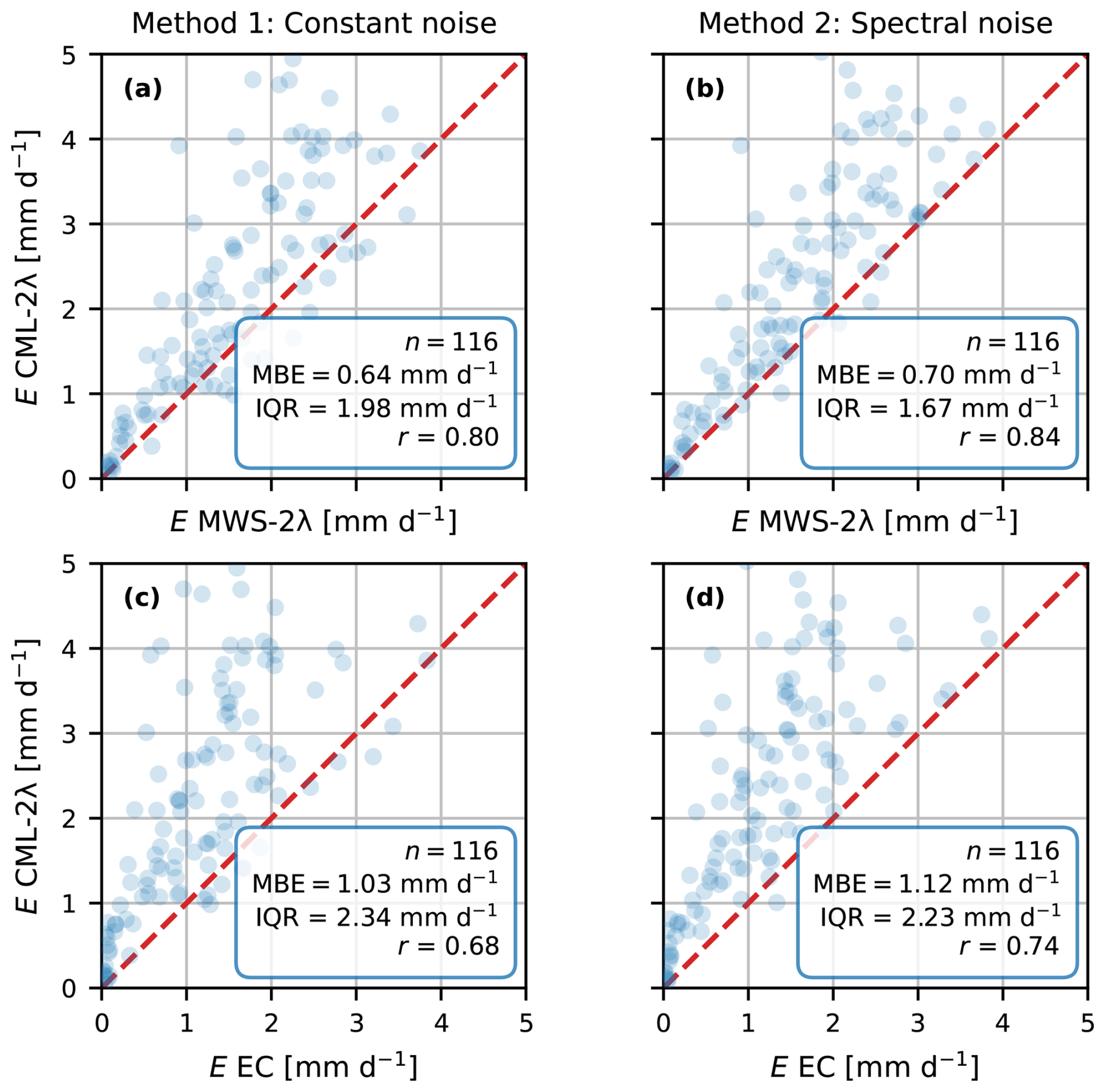
Figure 7 Comparison of daily E estimates obtained with the Nokia CML in combination with the LAS using the two-wavelength method for the entire study period, post-processed with the constant noise method (a, c) and spectral noise method (b, d) versus the MWS-2λ method (a, b) and the EC (c, d) estimates. The red line is the 1:1 line.

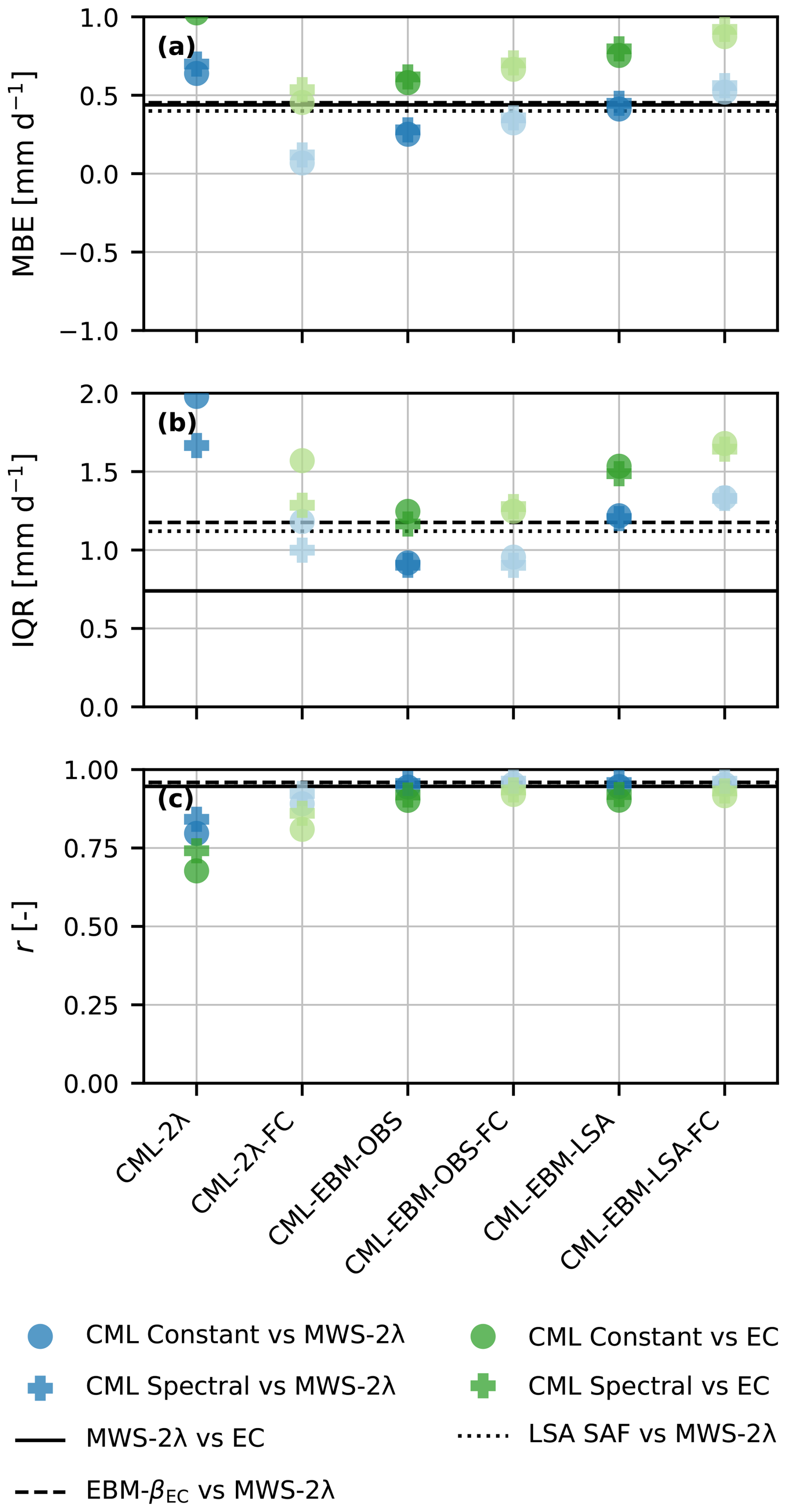
Figure 8 Statistical metrics per method and scaling to obtain daily E estimates using the Nokia CML for both correction methods (shape) versus both reference instruments (color). The solid line indicates the statistical metrics of the reference instruments versus each other (Fig. 3). CML-2λ method uses the two-wavelength scintillation method with the CML and LAS, CML-EBM-OBS uses the measured energy balance method as constraint to infer the turbulent heat fluxes and CML-EBM-LSA uses the estimated net radiation by LSA SAF instead of the measured net radiation. The “FC”-suffix refers to the free-convection scaling. The dotted line shows the statistical metrics of a comparison between the L_vE estimates directly obtained from LSA SAF versus the MWS-2λ method method. The dashed line represents L_vE estimates based on the measured available energy (R_net−G) and the Bowen ratio β obtained from the EC-system, i.e., $\frac{R_{\mathrm{net}}-G}{\mathrm{1}+\mathit{\beta }}$ versus the MWS-2λ method. The used Bowen ratio is a median value for the full data period (excluding nighttime intervals), as a means to obtain an objectively selected, representative Bowen ratio value to estimate L_vE from only net radiation measurements. We refer the reader to Appendix A for a complete overview of the used abbreviations.

5 Discussion

This study aims to obtain L_vE estimates using CMLs as scintillometers and builds on the correction methods proposed by van der Valk et al. (2025a). In that study, a formerly employed Nokia CML is used to obtain C_nn estimates by correcting the CML for the white noise floor in the received signal intensities using two proposed correction methods, a straightforward constant noise and a more advanced spectral noise method. In this study, we make use of both correction methods to obtain L_vE estimates from the estimated 30 min C_nn values with the same formerly employed Nokia CML. In general, all presented methods show that it is possible to obtain L_vE estimates using this Nokia CML. Moreover, conversion of the 30 min L_vE estimates to daily evaporation estimates keeps on average a similar bias.

5.1 Energy-balance method versus two-wavelength method

Similar to the C_nn estimates reported in van der Valk et al. (2025a), the spectral noise correction method outperforms the constant noise method for the L_vE estimates. As shown in van der Valk et al. (2025a), the spectral noise method mostly reduces the IQR in C_nn estimates, which is also reflected in our results. When using the two-wavelength method with the spectral noise method and free-convection scaling, the performance of the L_vE estimates is roughly comparable to the intercomparison between our reference instruments, the MWS-2λ method and EC system. Using the complete scaling instead, the performance of the L_vE estimates decreases, due to the overestimation of C_nn after correction (van der Valk et al., 2025a). The MWS-2λ method estimates larger L_vE values than the EC system, similar to Meijninger et al. (2002, 2006) and Ward et al. (2015a), while the spread in our comparison of the reference instruments is similar to these studies, too.

However, the two-wavelength method can usually not be applied for an entire CML network, due to the absence of a LAS. To overcome this limitation, the EBM proposed by Leijnse et al. (2007b) can be used, which requires net radiation as additional constraint and assumes closure of the measured energy balance. The L_vE estimates of the EBM-OBS are most similar to the reference instruments. Surprisingly, this method even outperformed the two-wavelength method, which is traditionally used in scintillometry. However, this method largely overestimates H, which reduces the overall performance of the EBM-OBS. For the two-wavelength method, the performance of the H estimates is comparable to the L_vE estimates and also comparable to the intercomparison of our reference methods (as the LAS is the main contributor to the H estimates in the two-wavelength method).

Moreover, net radiation is not frequently measured either, which motivated us to consider a satellite-derived radiation product as well. In our case, we use the LSA SAF radiation products and assume that 10 % of the net radiation is used for the ground heat flux. Generally, the net radiation obtained from LSA SAF overestimates the measured net radiation at Cabauw, so that the sum of the turbulent heat fluxes is also overestimated. This underlines the bottleneck of this method, in which the performance of the used net radiation product largely affects the performance of the turbulent heat fluxes, especially the MBE. For LSA SAF, Rains et al. (2024) finds over Europe an average underestimation of 9 W m⁻², with overall a relatively spatially homogeneous performance. However, in more complex environments the net radiation determination can be more difficult. Yet, the EBM-LSA does provide a decent estimate of L_vE, especially when considering it would allow to estimate L_vE using CMLs in places where other measurements are lacking. Other possibilities to obtain net radiation could be based on more basic meteorological measurements, such as suggested by Holtslag and Van Ulden (1983), but do require the use of multiple constants which depend on the local conditions.

Our results show the benefits of using CMLs to estimate L_vE, especially for the EBM-OBS. These EBM estimates show an improvement when comparing to L_vE estimates obtained from measured net radiation and a prescribed Bowen ratio, i.e., the median of the Bowen ratio measured by the EC over all used time intervals, predominantly by reducing the spread. Moreover, in comparison to L_vE estimates obtained from LSA SAF data product, the EBM-OBS shows an improvement, while EBM-LSA does not show any improvement in comparison to these LSA SAF L_vE estimates. Overall, this illustrates the potential of the EBM with measured net radiation, but also the dependence of this method on the quality of the measured net radiation estimates.

However, application of the EBM is not trivial in general, let alone over complex terrain, such as cities or forests. Typically, the observed energy balance does not close (Mauder et al., 2020), which is also the case for our field site (Kroon, 2004). For cities the addition of the anthropogenic heat flux as heat source for the turbulent heat fluxes (e.g., Oke et al., 2017) and the significant amount of heat storage (e.g., Sun et al., 2017) can complicate the application of the EBM (e.g., Harman and Belcher, 2006; Miao et al., 2012). These fluxes are added to the energy balance, so that the assumed energy balance for the EBM versions is not valid for every CML in cities. Moreover, the validity of the EBM also depends on the location of the CML, for example the mounting height, which affects the footprint of the CML to be on local scales, i.e., streets for cities, or more regional scales, i.e., city (or neighbourhood) scales.

5.2 MOST L_vE estimates versus free-convection

The complete MOST scaling requires temperature, humidity and horizontal wind speed measurements and estimates of the roughness length. To eliminate the dependency on horizontal wind speed and roughness length, we apply the free-convection scaling. These eliminated variables have a relatively large influence on the performance of the L_vE estimates, especially for large C_nn values, and thus L_vE (Leijnse et al., 2007b; Ward et al., 2014). Additionally, these variables can be relatively hard to measure in complex environments and would require a more elaborate setup. On the other hand, the use of free-convection scaling introduces an underestimation of the turbulent heat fluxes by assuming that turbulence is only buoyancy-driven and neglecting the shear-driven part, which is confirmed by our findings for the two-wavelength method, similar to Kohsiek (1982) and De Bruin et al. (1995). Moreover, typical mounting heights of CMLs are at least around 20–30 m above the surface, so that $-\frac{z}{L_{\mathrm{Ob}}}$ increases in comparison to our setup and the underestimation of the turbulent heat fluxes reduces. However, it must be noted that for the EBM versions, the use of free-convection causes an increase in the L_vE estimates and a reduction in H in comparison to the complete scaling. H reduces due to the strong relation with the free-convection wind scaling variable u_fc (Eq. 11), which decreases compared to the friction velocity u_*, so that L_vE has to increase as a consequence of the prescribed available energy that needs to be distributed among the two turbulent heat fluxes.

For both scaling methods information on r_Tq is required, in order to determine C_TT and C_qq. The value of r_Tq can be determined by using the bichromatic method proposed by Lüdi et al. (2005) or using an EC system or, alternatively, a value has to be assumed (although for flows following MOST, r_Tq has to be equal to one for two conservative scalars; Hill, 1989). The bichromatic method is not applicable to the Nokia CML, given the large amount of noise added to the signal. In our case, we assumed r_Tq to be equal to 0.8, following the recommendations of Ward et al. (2015b). Previous studies suggest r_Tq to be just below 1 during the day for many different types of surface (e.g., Kohsiek, 1982; Priestley and Hill, 1985; Andreas et al., 1998; Beyrich et al., 2005; Ward et al., 2015b), while an intercomparison of multiple studies by Andreas (1987) revealed a maximum around 0.8. Moreover, Ward et al. (2015b) reports a decrease in maximum r_Tq values for their setup during winter months towards approximately 0.5, while Leijnse et al. (2007b) report a relatively high sensitivity of L_vE estimates to r_Tq for low C_nn values. So, when assuming r_Tq values for application in CML networks a seasonally-dependent value could result in improved L_vE estimates, even though it should be noted that L_vE during winter months is relatively low. Overall, assuming that r_Tq equals 0.8 during the day seems a reasonable estimate, especially when focusing on evaporation during the evaporation season.

5.3 Potential of CMLs to estimate L_vE

Extrapolation of our results to CML networks is not directly possible. Firstly, not all CML antennas modify the received signal intensity in the same manner. For example, in van der Valk et al. (2025a), we rejected a formerly employed Ericsson CML, due to the 0.5 dB power quantization by the antenna. Next to this quantization, CML data is typically not provided at 20 Hz, but either a minimum and maximum signal intensity value per 15 min time interval or an instantaneous value every second to minute. Also, other types of CML antennas might have different noise floors than the Nokia CML.

Secondly, we have tested our methods for Cabauw, the Netherlands, where the water table is managed and with relatively idealized conditions. For example, the Bowen ratio is relatively constant throughout the entire year. Generally, microwave scintillometry has proven itself as reliable method to estimate L_vE over different landscapes, such as heterogeneous farmlands (e.g., Meijninger et al., 2002, 2006; Beyrich et al., 2005; Xu et al., 2023), cities (Ward et al., 2015a). Also, in areas with a more complex topography, scintillometry has shown its value for estimating the turbulent heat fluxes, especially on larger-scales, such as over vineyards (Perelet et al., 2022) or hilly forests (Isabelle et al., 2019). For H, several studies, some only using an optical scintillometer, have shown the potential over heterogeneous farmland (e.g., Beyrich et al., 2002; Ezzahar et al., 2007), arid regions with sparse vegetation (e.g., Asanuma and Iemoto, 2007; Kleissl et al., 2009), and cities (e.g., Lagouarde et al., 2006; Lee et al., 2015). Yee et al. (2015) compares several scintillometers and methods and identifies the difficulty using the two-wavelength method and EBM for higher Bowen ratios. For microwave scintillometry in dryer environments, Wesely (1976), Moene (2003), Leijnse et al. (2007b) and Ward et al. (2015b) emphasize the importance of correctly estimating r_Tq. Moreover, at Bowen ratios around 2–3, C_nn at microwave wavelengths can theoretically approach zero (for $r_{Tq}=\pm \mathrm{1}$), due to the C_Tq term in Eq. (1) canceling the C_TT and C_qq terms (Hill et al., 1988; Leijnse et al., 2007b; Ward et al., 2013). If so, the actual C_nn values may drop below the detection limit of the scintillometer, due to the noise floor in receiving antennas. Our correction methods, in which we try to reduce the noise floor as much as possible, will likely also encounter difficulties for such Bowen ratios.

Future research to estimate evaporation using CMLs should focus on the typically employed sampling strategies of CMLs in communication networks, signal intensity modification by antennas and perhaps explore more opportunistic methods. Obtaining realistic C_nn from less frequently sampled signal intensities is complicated due to the undersampling of part of the turbulent power spectrum. Moreover, different noise floors in antennas or power quantization of the signal intensity also complicate C_nn computation.

6 Conclusions

In this study, we investigated the use of former CMLs to obtain 30 min L_vE and daily E estimates through scintillometry. We build on the results of van der Valk et al. (2025a), who obtained C_nn estimates by correcting a formerly employed Nokia CML for its noise floor. We computed L_vE estimates using the conventional two-wavelength method and a standalone method which prescribes the available energy for the turbulent heat fluxes based on net radiation, and compared these with an actual two-wavelength scintillometer setup and an EC system. Using the two-wavelength method, the performance of the turbulent heat flux estimates obtained with the free-convection scaling and spectral noise correction method is roughly comparable to the comparison between the reference MWS-2λ method and EC system, while application of the two-wavelength method combined with the complete scaling performs less well. In line with the C_nn estimates of van der Valk et al. (2025a), the spectral noise method reduces the spread in comparison to the constant method. For example, for the two-wavelength method using the complete scaling the IQR reduces from 154 to 134 W m⁻² when comparing to the MWS-2λ method. However, application of the two-wavelength method is not possible for entire CML networks, as it would require installation of a LAS next to every CML.

As standalone alternative, the EBM versions require net radiation estimates as a constraint, so that this can be distributed over L_vE and H. The EBM using measured radiation seems to outperform the two-wavelength for the L_vE estimates, but the H estimates are worse. As an alternative to the radiation measurements, we used the LSA SAF radiation products to estimate the net radiation. The overestimation and uncertainty of the net radiation by LSA SAF in comparison to the measured net radiation is also reflected in the performance of our turbulent heat fluxes. The MBE and IQR of the latent heat flux estimates using the constant noise method and complete scaling increases from 20 to 33 W m⁻² and from 130 to 170 W m⁻² in comparison to the MWS-2λ method, respectively. Overall, this illustrates the dependence of the performance of the EBM versions on the quality of the net radiation data, while the assumption of closure of the measured energy balance is not always valid either. For example, over complex environments, such as cities or forest, additional uncertainties are introduced for this method.

The complete scaling of Monin-Obukhov requires temperature, humidity and wind speed measurements, and assumptions on the roughness length, next to C_nn (and the net radiation for the EBM). To eliminate the need for wind speed measurements and roughness length assumptions, we apply free-convection scaling instead of the complete scaling. This scaling neglects the shear-driven part of the turbulent heat fluxes, so that typically the fluxes tend to be underestimated. For our study, this results in an average reduction of the latent heat flux estimates of 40 W m⁻² for the two-wavelength method with the spectral noise correction method. For the EBM versions, this underestimation is generally not applicable, since the method prescribes the amount of energy that needs to be distributed among the latent and sensible heat fluxes. For our experiment, this results in an increase in bias for the latent heat flux and a reduction in sensible heat flux estimates, with similar patterns emerging for the spread.

In general, our results illustrate the possibility to use CMLs as scintillometers. Also after aggregation of the 30 min L_vE estimates to daily E estimates, the performance remains comparable for almost all methods and days. This aggregation might be particularly interesting for hydrological applications, for example on spatial scales of catchments, which could be combined with the possibility to monitor rainfall using the same CMLs. However, our results also illustrate that the accuracy of the L_vE estimates using CML networks will largely depend on the quality of the radiation estimates. The quality of widely available radiation data, such as LSA SAF, seems too low for our purposes, and needs to be addressed in future research. Additionally, attempts to estimate evaporation using different CML types and employed sampling strategies of networks would be required, while also the performance of the proposed methods and scalings need to be tested in different climatic settings. If these issues would be addressed, CMLs could show a large potential to be used to estimate evaporation, especially considering the existing infrastructure which is also present on locations where other observations are lacking.

Appendix A: Abbreviation list

Table A1 List of used abbreviations.

Appendix B: Net radiation LSA SAF versus measurements

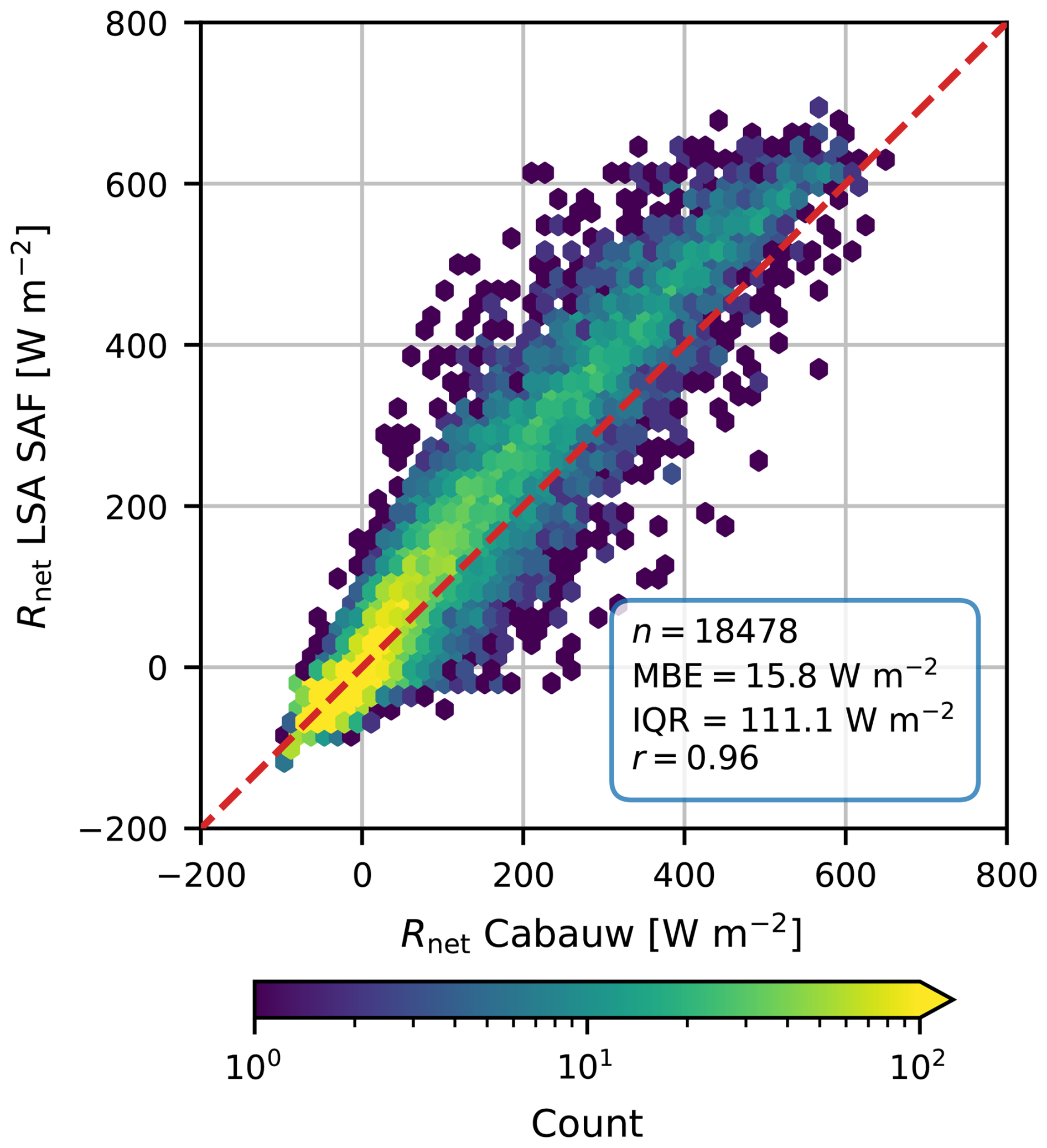
Figure B1 Comparison of 30 min R_net estimates using LSA SAF versus the net radiation measured at Cabauw for our data period.

Appendix C: Statistics H

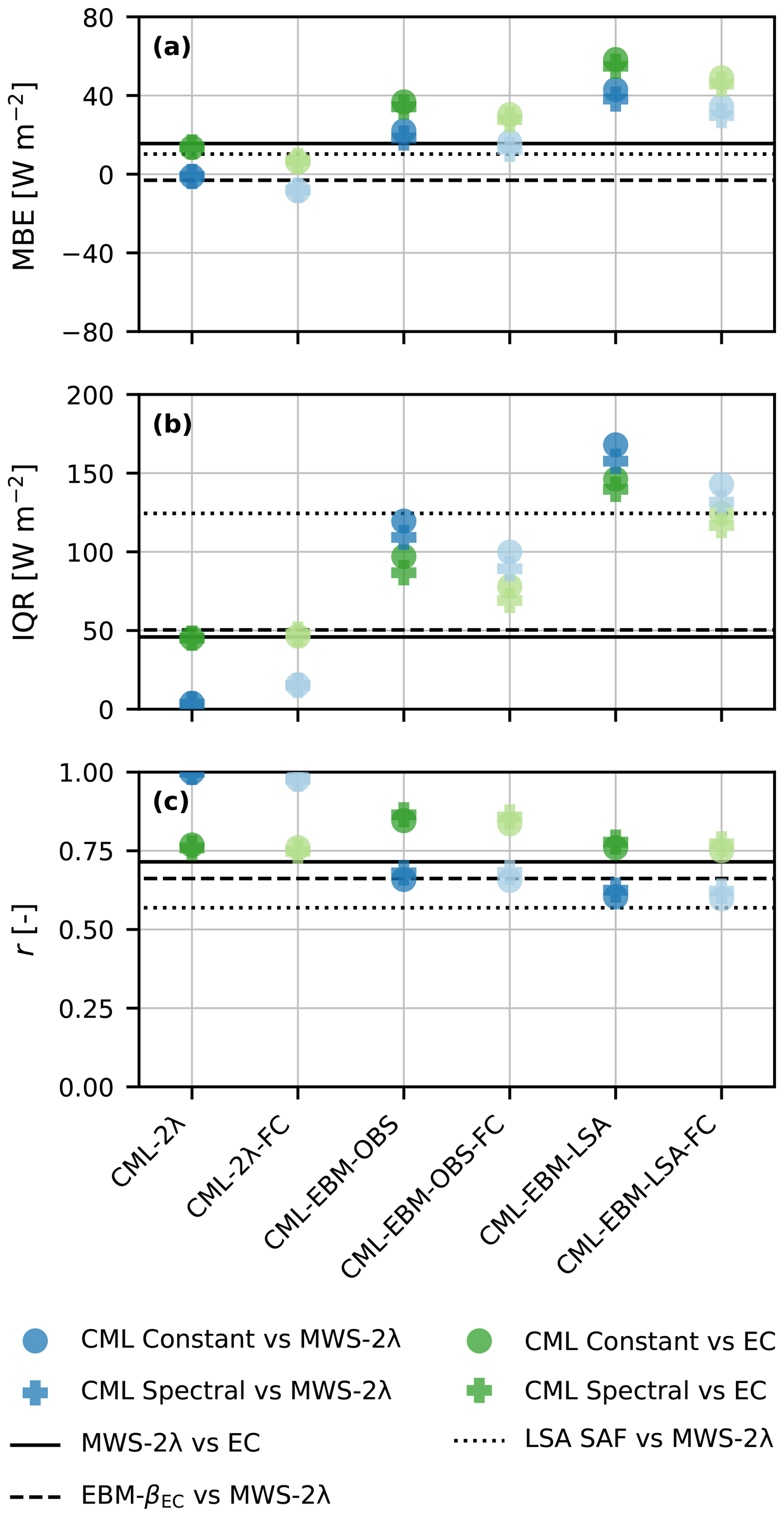
Figure C1 Statistical metrics per method to obtain H estimates using the Nokia CML for both correction methods (shape) versus both reference instruments (color). The solid line indicates the statistical metrics of the reference instruments versus each other. CML-2λ method uses the two-wavelength scintillation method with the CML and LAS, CML-EBM-OBS uses the measured energy balance method as constraint to infer the turbulent heat fluxes and CML-EBM-LSA uses the estimated net radiation by LSA SAF instead of the measured net radiation. The “FC”-suffix refers to the free-convection scaling. The dotted line shows the statistical metrics of a comparison between the H estimates directly obtained from LSA SAF versus the MWS-2λ method. The dashed line represents H estimates based on the measured available energy (R_net−G) and the Bowen ratio β obtained from the EC-system, i.e., $\frac{\mathit{\beta }(R_{\mathrm{net}}-G)}{\mathrm{1}+\mathit{\beta }}$ versus the MWS-2λ. The used Bowen ratio is a median value for the full data period (excluding nighttime intervals), as a means to obtain an objectively selected, representative Bowen ratio value to estimate H from only net radiation measurements. We refer the reader to Appendix A for a complete overview of the used abbreviations.