the Creative Commons Attribution 4.0 License.
the Creative Commons Attribution 4.0 License.
 | 04 Feb 2025
Modeling Lake Titicaca's water balance: the dominant roles of precipitation and evaporation
Nilo Lima-Quispe
Denis Ruelland
Antoine Rabatel
Waldo Lavado-Casimiro
Thomas Condom
In the face of climate change and increasing anthropogenic pressures, a reliable water balance is crucial for understanding the drivers of water level fluctuations in large lakes. However, in poorly gauged hydrosystems such as Lake Titicaca, most components of the water balance are not measured directly. Previous estimates for this lake have relied on scaling factors to close the water balance, which introduces additional uncertainty. This study presents an integrated modeling framework based on conceptual models to quantify natural hydrological processes and net irrigation consumption. It was implemented in the Water Evaluation and Planning System (WEAP) platform at a daily time step for the period 1982–2016, considering the following terms of the water balance: upstream inflows, direct precipitation and evaporation over the lake, and downstream outflows. To estimate upstream inflows, we evaluated the impact of snow and ice processes and net irrigation withdrawals on predicted streamflow and lake water levels. We also evaluated the role of heat storage change in evaporation from the lake. The results showed that the proposed modeling framework makes it possible to simulate lake water levels ranging from 3808 to 3812 m a.s.l. with good accuracy (RMSE = 0.32 m d−1) over a wide range of long-term hydroclimatic conditions. The estimated water balance of Lake Titicaca shows that upstream inflows account for 56 % (958 mm yr−1) and direct precipitation over the lake for 44 % (744 mm yr−1) of the total inflows, while 93 % (1616 mm yr−1) of the total outflows are due to evaporation and the remaining 7 % (121 mm yr−1) to downstream outflows. The water balance closure has an error of −15 mm yr−1 without applying scaling factors. Snow and ice processes, together with net irrigation withdrawals, had a minimal impact on variations in the lake water level. Thus, Lake Titicaca is primarily driven by variations in precipitation and high evaporation rates. These results will be useful for supporting decision-making in water resource management. We demonstrate that a simple representation of hydrological processes and irrigation enables accurate simulation of water levels. The proposed modeling framework could be replicated in other poorly gauged large lakes because it is relatively easy to implement, requires few data, and is computationally inexpensive.
- Article
(8371 KB) - Full-text XML
- BibTeX
- EndNote


1.1 On the need for an integrated water balance in large lakes
Lakes are water reservoirs of vital importance for the development of regions as they provide many ecosystem services, including fisheries, water supply, tourism, and energy generation (Sterner et al., 2020). However, these services can be impacted by fluctuating lake water levels. For instance, Yao et al. (2023) showed that, in the period from 1992 to 2020, there was a significant decrease in water levels in 43 % of natural lakes (457), an increase in 22 % (234), and nonsignificant trends in 35 % (360). Understanding the main drivers of fluctuations in water levels is crucial for effective lake management, which requires a realistic water balance that accounts for both natural processes and anthropogenic pressures (Wurtsbaugh et al., 2017). Several studies on large lakes (> 500 km2) (e.g., Rientjes et al., 2011; Vanderkelen et al., 2018; Wale et al., 2009) have estimated water balance under the assumption that net water withdrawals in the contributing catchments are negligible. However, this assumption may no longer be valid due to changing climate conditions and increased competition for water uses, potentially leading to reduced upstream inflow (Wurtsbaugh et al., 2017). For example, Schulz et al. (2020) demonstrated that net withdrawals for irrigation exacerbate the decline in storage at Lake Urmia, which is also impacted by climate change.
In large lakes, it is essential to adopt integrated water balance modeling, which represents the interactions and feedbacks between natural hydrological processes and water management within a single modeling framework (Niswonger et al., 2014). Unlike traditional decision support systems applied to large lakes (Hassanzadeh et al., 2012), which typically simulate natural flows and irrigation water requirements independently, integrated modeling enables these processes to be simulated in a coupled and dynamic manner. A few studies have attempted to address an integrated water balance in a large lake hydrosystem (e.g., Hosseini-Moghari et al., 2020; Lima-Quispe et al., 2021). These studies tend to focus on some components of the water balance, while others address them superficially. For example, Hosseini-Moghari et al. (2020) focused on estimating the upstream inflow of Lake Urmia, with less emphasis on direct precipitation over the lake and evaporation, which both play very important roles in the water balance of large lakes (Gronewold et al., 2016). This is partly because large lake hydrosystems involve numerous hydrological processes, and there are often insufficient data to represent these processes in detail and evaluate them comprehensively. The issue is further complicated in transboundary lake hydrosystems, where hydrometeorological monitoring is not always coordinated (Gronewold et al., 2018).
1.2 Challenges in estimating the water balance of large lakes
It is widely recognized that large lakes have a major influence on regional climate (Scott and Huff, 1996; Su et al., 2020). For example, it has been observed that direct precipitation over the African Great Lakes is more intense than in their surrounding areas (Anyah et al., 2006; Kizza et al., 2012; Nicholson, 2023; Thiery et al., 2015). According to Scott and Huff (1996), this is due to the differences in heat capacities between the lake surfaces and the surrounding areas as well as the large amount of moisture that lakes provide for the lower atmosphere, which can lead to increased cloudiness and precipitation over lakes. Estimating precipitation based on ground stations, which are mainly located in the surrounding areas, can lead to inaccuracies. Despite the current availability of remotely sensed datasets, they have been shown to still have significant biases (Hong et al., 2022; Satgé et al., 2019). Regarding direct evaporation, this depends not only on meteorological conditions, but also on the size of the lake, water depth, and water clarity, which all influence the energy balance due to changes in water temperature and vertical mixing (Lenters et al., 2005). Thus, estimating lake evaporation based on meteorological data alone can lead to inaccuracies (Bai and Wang, 2023). The energy balance method is considered to be one of the most appropriate and accurate for estimating evaporation (Lenters et al., 2005) but requires large quantities of data, meaning that it is generally difficult to implement. The original Penman formulation, which does not include changes in heat storage, has been used to estimate lake evaporation (e.g., Kebede et al., 2006; Lima-Quispe et al., 2021). However, Blanken et al. (2011) observed a 5-month delay between peak net radiation and evaporation due to heat storage in Lake Superior in North America. One of the limitations of estimating the change in heat storage is the lack of water temperature data at different depths, and so models are used to simulate the thermal stratification dynamics of the water (e.g., Antonopoulos and Gianniou, 2003).
For upstream inflow, ideally, measured streamflow data will be available. However, there are always ungauged catchments contributing to lakes (Wale et al., 2009). Upstream inflow is mostly estimated with hydrological models (e.g., Rientjes et al., 2011; Zhang and Post, 2018). For the ungauged catchments, regionalization methods are applied based on the parameters obtained in the gauged catchments (e.g., Guo et al., 2021). Basic lumped rainfall-runoff simulations may fall short due to the complex interplay of natural hydrological processes and water management. Integrating both aspects is essential for hydrosystems under significant anthropogenic pressure (e.g., Ashraf Vaghefi et al., 2015; Fabre et al., 2015; Hublart et al., 2016). In high mountain catchments, snow and ice processes significantly impact hydrological responses. Estimating melt is challenging because it is difficult to obtain accurate forcing data (e.g., precipitation and temperature) in high-elevation areas where the measurement network is very sparse (Ruelland, 2020) as well as control data (e.g., upstream-area streamflow and glacier mass balance). In this context, temperature-index approaches (Hock, 2003) are more suitable than energy balance approaches and can produce simulations with acceptable accuracy using a reduced number of parameters and forcing data (e.g., Ruelland, 2023). In terms of water management, according to Wu et al. (2022), 60 % of freshwater withdrawals worldwide are made for agricultural irrigation. Catchment-scale irrigation has been addressed using approaches based on soil water deficit (Kannan et al., 2011; Shadkam et al., 2016) and those that additionally consider irrigation scheduling (Githui et al., 2016; McInerney et al., 2018). Regardless of the approach chosen, one of the limitations is the lack of measured irrigation data (McInerney et al., 2018), which hinders the evaluation of irrigation simulations. This evaluation can consequently only be undertaken indirectly by attempting to more realistically reproduce observed outlet discharges and accounting for net consumption for water uses within the catchments (e.g., Fabre et al., 2015; Hublart et al., 2016).
Net groundwater exchanges are neglected in some studies under the assumption that these fluxes are very small (Duan et al., 2018; Lima-Quispe et al., 2021). Lake–groundwater interactions have been addressed using conceptual (Parizi et al., 2022) and physically based models (Vaquero et al., 2021; Xu et al., 2021), chemical and isotopic balances (Bouchez et al., 2016), and the water balance (Chavoshi and Danesh-Yazdi, 2022). The water balance is a fairly easy option, as the net flux is the result of the other components. However, it is crucial to dispose of accurate measurements or estimates of the other water balance terms to avoid propagating uncertainty (Chavoshi and Danesh-Yazdi, 2022). Hydrochemical or isotopic analyses are considered accurate (Bouchez et al., 2016) but can be very costly for a large lake. Modeling approaches are often limited by data availability (Barthel and Banzhaf, 2016), particularly when using models to dynamically simulate surface water–groundwater interactions (Xu et al., 2021). On the other hand, downstream outflow in exorheic lakes can be estimated by direct measurements (Chebud and Melesse, 2009), a rating curve relating lake level to outflow (Sene and Plinston, 1994), and as a residual of the water balance (Duan et al., 2018).
1.3 Placing Lake Titicaca in the context of an integrated water balance
Lake Titicaca, located on the Altiplano of the tropical Andes of South America, is one of the highest large lakes in the world and an interesting case study for an integrated water balance. This lake is part of a vast endorheic catchment and is connected by the Desaguadero River to Lake Poopó in Bolivia (see Fig. 1) (Lima-Quispe et al., 2021). As a transboundary lake shared by Peru and Bolivia and as a poorly gauged hydrosystem, it faces many of the aforementioned challenges. The region experiences significant interannual climate variability (Garreaud and Aceituno, 2001), which, coupled with complex water management issues (Revollo, 2001), intensifies the difficulties in managing Lake Titicaca. These challenges include extreme hydrological events (droughts and floods), lake releases, and water pollution (Revollo, 2001; Rieckermann et al., 2006). Water levels measured in Puno (Peru) have fluctuated by approximately 6 m over the past century, with the lowest recorded in 1943–1944 and the highest recorded in 1984–1986 (Sulca et al., 2024), causing USD 125 million in flood damage (Revollo, 2001). In response to these challenges, a management plan was developed in the early 1990s for both Lake Titicaca and the Altiplano hydrosystem (Revollo, 2001). A key component of this plan was the construction of an outflow gate to regulate lake releases and the establishment of operating rules. Although the outflow gate was completed in 2001, lake releases remain nearly the same as under natural conditions because the operating rules have not yet been implemented. Addressing these water management challenges requires an accurate integrated water balance allowing better knowledge of the drivers of the lake water level variations.
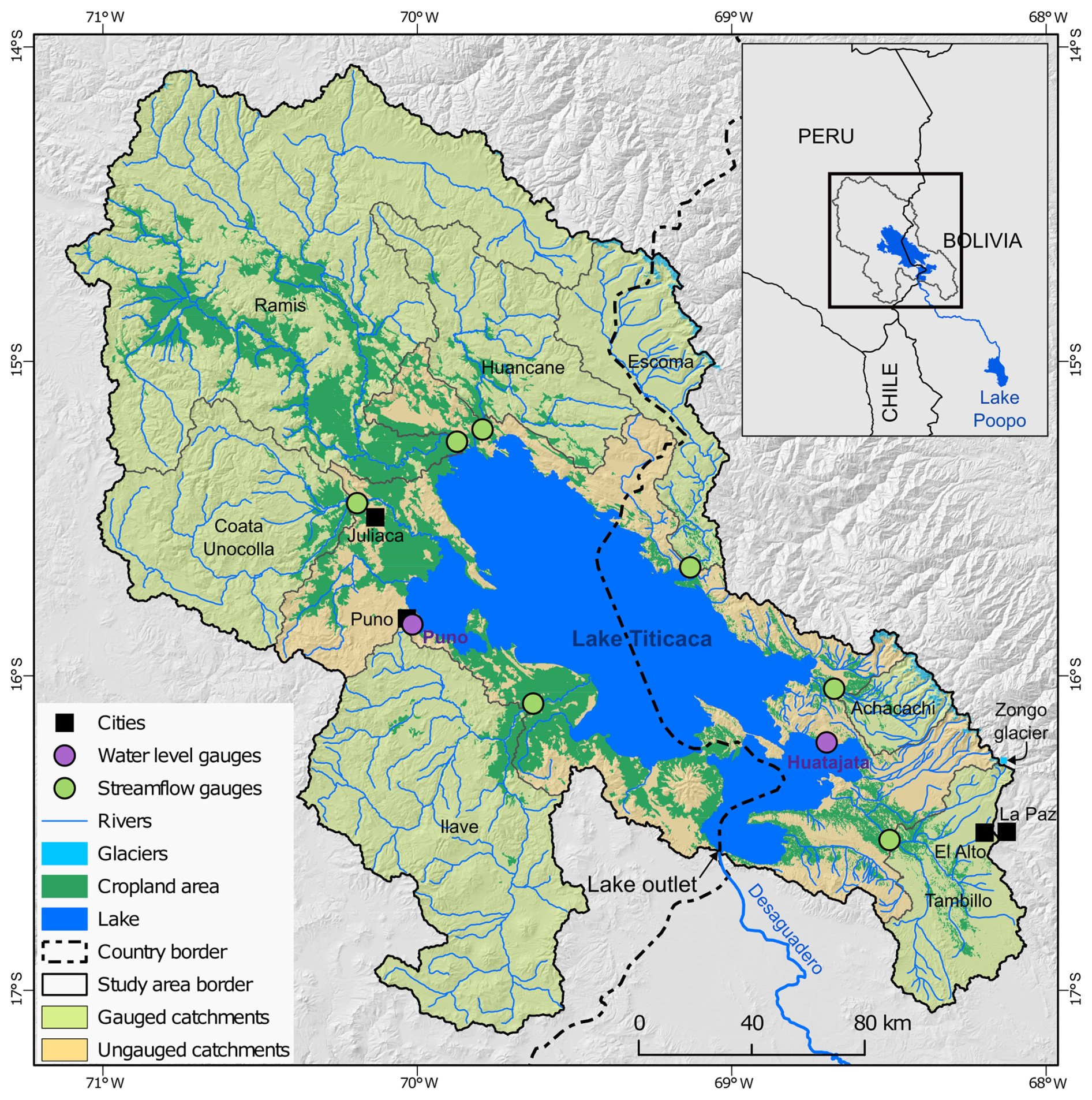
Figure 1The main geographical features of the Lake Titicaca hydrosystem and the locations of the main streamflow gauges. The reference year for the limits of the glacier is 2000 (RGI Consortium, 2017). The reference year for the croplands is 2010 (Ministerio de Desarrollo Rural y Tierras, 2011; Ministerio del Ambiente, 2015).
Unlike other large lakes, very few studies have been conducted on Lake Titicaca. The only study modeling the water balance of Lake Titicaca and Lake Poopó was the one by Lima-Quispe et al. (2021) using the Water Evaluation and Planning System (WEAP) platform with a monthly time step for the period 1980–2015. The study aimed to distinguish between the relative contributions of climate and irrigation management to water level fluctuations. However, the modeling approach proposed by the authors has a significant limitation because it is based on a scaling factor for precipitation over the lake to close the water balance, which clearly introduces additional uncertainty. Other methodological shortcomings include (i) the omission of snow and ice processes, which can play a non-negligible role in this high-elevation region; (ii) the estimation of evaporation using the Penman method, without accounting for changes in heat storage; and (iii) the use of historical monthly averages (humidity, wind speed, and incoming solar radiation) to calculate reference evapotranspiration and evaporation, without considering interannual variability.
1.4 Scope and objectives
In addressing the challenges and limitations of representing hydrological processes in poorly gauged large lakes such as Lake Titicaca, we pose the following key question: how can a reliable water balance be estimated? To answer this, we present an integrated modeling framework based on conceptual models to estimate the water balance of Lake Titicaca more reliably. The modeling framework is applied at a daily time step for the period 1982–2016, allowing us to represent water level fluctuations over a wide range of hydroclimatic conditions. The specific questions are the following: to what extent are water level variations sensitive to net irrigation withdrawals and to snow and ice processes? What is the role of heat storage change in evaporation from the lake? To address these questions, new approaches are introduced for (i) predicting upstream inflow, including hydrological sensitivity to net irrigation consumption and snow and ice processes; and (ii) estimating evaporation from the lake using the Penman method while accounting for changes in heat storage.
2.1 The Lake Titicaca hydrosystem
Lake Titicaca, located at 3812 m a.s.l. on the Altiplano of the tropical Andes of South America, covers an area of approximately 8340 km2. The elevation of the catchments that contribute to the lake ranges between 3812 and 6300 m a.s.l. (average 4200 m a.s.l.) and covers an area of approximately 48 780 km2. The lake has an average volume of 958 km3 and a maximum depth of 277 m according to the bathymetry carried out between 2016 and 2019 (Autoridad Binacional del Lago Titicaca, 2021). Lake Titicaca is of regional hydrological importance, and the outflows of Lake Titicaca represent up to 79 % of the inflows of Lake Poopó (Lima-Quispe et al., 2021). The Lake Titicaca Authority (Spanish abbreviation ALT) was also created as an autonomous binational entity with the mission of managing the lake.
2.2 Climate data
Daily precipitation and air temperature (see Fig. 2) were obtained from the data generated in Bolivia (Ministerio de Medio Ambiente y Agua, 2018) with the Gridded Meteorological Ensemble Tool (GMET) (Clark and Slater, 2006; Newman et al., 2015). GMET has a spatial resolution of 0.05° for the period 1980–2016. It is based on a probabilistic method using ground station data, with further details provided by Clark and Slater (2006) and Newman et al. (2015). Lima-Quispe et al. (2021) used the same data. In some catchments in the study area, Satgé et al. (2019) evaluated 12 satellite-based products and found that MSWEP and CHIRPS products were the most promising at the 10 d time step. As a result, for daily precipitation, four datasets, i.e., GMET, MSWEP, CHIRPS, and basic interpolation of ground station data with inverse distance weighting (IDW) (Ruelland, 2020), were initially tested according to daily hydrological sensitivity analyses. The results showed that GMET led to more accurate simulations in most catchments and Lake Titicaca (not shown here for the sake of brevity). Daily data on relative humidity, wind speed, and solar radiation are very scarce in space and over time. Many values were missing in the time series from the weather stations, thus calling their quality and representativeness into question. For this reason, we used reanalysis data from ERA5-Land (Muñoz-Sabater et al., 2021) (see Appendix A).
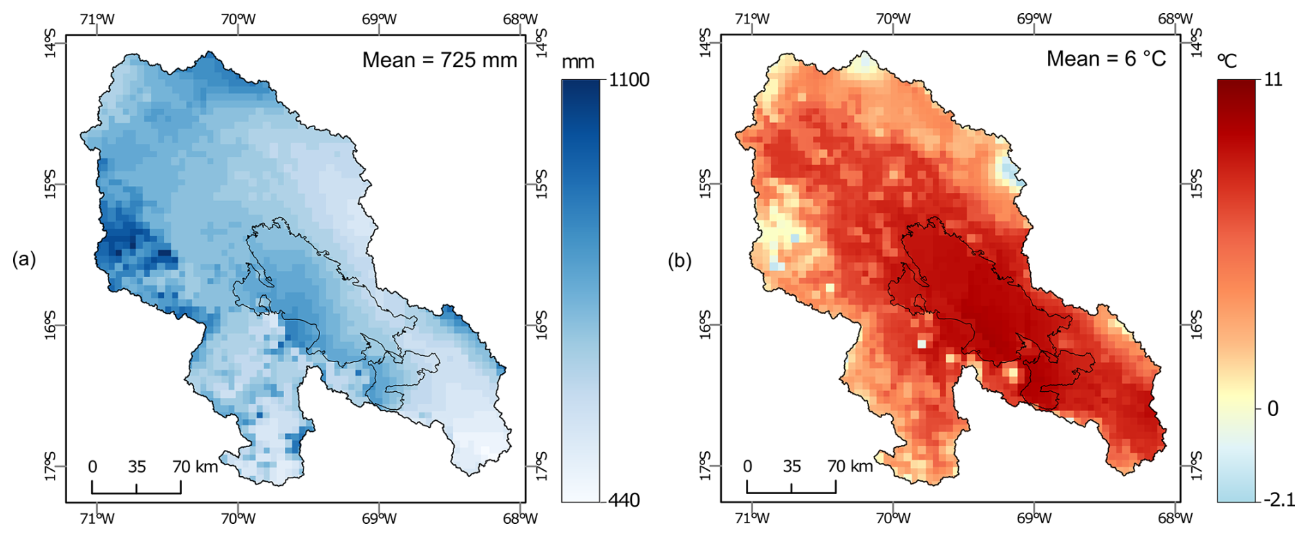
Figure 2Spatial distribution of (a) annual precipitation and (b) mean temperature for the hydrological period 1980–2016 according to GMET (Gridded Meteorological Ensemble Tool).
Figure 2 shows the spatial pattern of precipitation (see Fig. 2a) and air temperature (see Fig. 2b) based on GMET for the period 1980–2016. Annual precipitation varies between 440 and 1100 mm (mean 725 mm). The wettest areas are concentrated in the northwest and over Lake Titicaca. The driest areas are to the south. The spatial distribution does not show generalized dependence on elevation, but there are small areas on the eastern and western margins where precipitation increases with elevation. The annual mean air temperature varies between −2 and 11 °C (average 6 °C). The coldest areas are the western and eastern areas, coinciding with the highest mountains. The warmest areas are located over Lake Titicaca. The spatial distribution of the air temperature depends on the elevation.
2.3 Snow and glacierized areas
According to MODIS snow cover (Hall et al., 2002) computed over the period 2000–2016 based on a method described in Ruelland (2020), 80 % of the upstream catchments are completely free of snow throughout the year. Areas where the snow cover persists for more than 20 % of the year are located above 4700 m a.s.l. These high-elevation areas represent less than 0.5 % of the total surface area. Glacierized areas are located above 4600 m a.s.l. and represented 231 km2 in the early 2000s (RGI Consortium, 2017), i.e., less than 0.5 % of the total area. The estimated glacier volume is ∼ 12 km3 (Farinotti et al., 2019), which represents ∼ 1.3 % of the mean volume of Lake Titicaca (958 km3).
2.4 Croplands and irrigable area
According to land cover maps (Ministerio de Desarrollo Rural y Tierras, 2011; Ministerio del Ambiente, 2015) (see Fig. 1), cropland covers 8069 km2 (17 % of the upstream catchments). Agriculture is largely traditional, rainfed, and constrained by droughts, frosts, and hailstorms (Garcia et al., 2007). The main crops include forage grasses, potatoes, grain barley, and quinoa (INTECSA et al., 1993c). Only 40 % of arable land is cultivated due to crop rotation and agroclimatic constraints (INTECSA et al., 1993c). Potatoes are planted in October–November and harvested after 6 months, while quinoa has a similar cycle. Beans and onions, mostly irrigated, are planted from July to September. The land cover maps (Ministerio de Desarrollo Rural y Tierras, 2011; Ministerio del Ambiente, 2015) do not distinguish between rainfed and irrigated areas (see Fig. 1), limiting the identification of changes in irrigated areas over time. The ESA CCI-LC dataset (ESA, 2017) also does not identify irrigated areas in the Altiplano.
The available data come from the inventory of irrigation systems. The inventory on the Bolivian side was created in 2012 (Ministerio de Medio Ambiente y Agua, 2013). For the Peruvian side, the rights of use granted by the Autoridad Nacional del Agua (ANA) until 2023 were used (https://snirh.ana.gob.pe, last access: 12 May 2023). These inventories provide information on location (latitude and longitude), irrigable area, and volume granted (Peru) or a reference volume of irrigation (Bolivia). Figure 3 illustrates the irrigation systems in terms of location and irrigable area. The irrigable area is 767 km2 (see Table 1), which represents 1.6 % of the upstream catchments that contribute to Lake Titicaca. Only 9.5 % of the croplands are located in “irrigable areas”, i.e., cropland within the area of influence of an irrigation system that can potentially be irrigated. However, not all of the irrigable area is irrigated because irrigation depends on the availability of water in space and over time. Then, we assumed that the irrigable area was constant over the period 1980–2016. Figure 3 also shows that most of the irrigation systems cover an area of less than 5 ha; i.e., small-scale irrigation predominates. Also, irrigation is mostly practiced by smallholder farmers. Furrow irrigation is the most common system, and its efficiency is about 35 % (Autoridad Nacional del Agua, 2009; Instituto Nacional de Recursos Naturales, 2008; Ministerio de Medio Ambiente y Agua, 2013). The main sources of water are rivers and reservoirs (see Fig. 3). The main reservoir is Lagunillas (see Fig. 3), with a capacity of 500×106 m3. The remaining 15 reservoirs have capacities of less than 30×106 m3. Due to a lack of data on dam management, streamflow regulation was not accounted for, assuming that it has minimal impact on natural flows.
Table 1Main characteristics of the gauged and ungauged catchments that contribute to the lake. Glacier area was estimated using RGI 6.0 glacier outlines (RGI Consortium, 2017). Cropland area (including rainfed and irrigated area) was estimated using the 2010 land cover maps of Peru and Bolivia (Ministerio de Desarrollo Rural y Tierras, 2011; Ministerio del Ambiente, 2015). Irrigable area was estimated using data from the inventories of agricultural land use rights (Peru) (https://snirh.ana.gob.pe, last access: 12 May 2023) and irrigation systems (Bolivia) (Ministerio de Medio Ambiente y Agua, 2013). The reference year for irrigable area in Bolivia is 2012, and in Peru it has been updated to 2023. Elevations were extracted from a digital elevation model (DEM) at 90 m spatial resolution from the Shuttle Radar Topographic Mission (SRTM; Jarvis et al., 2008).
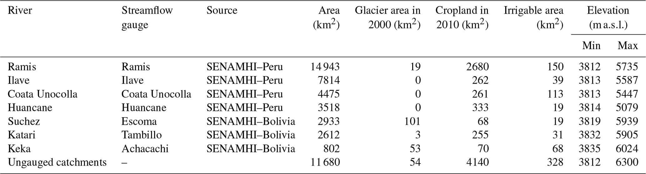
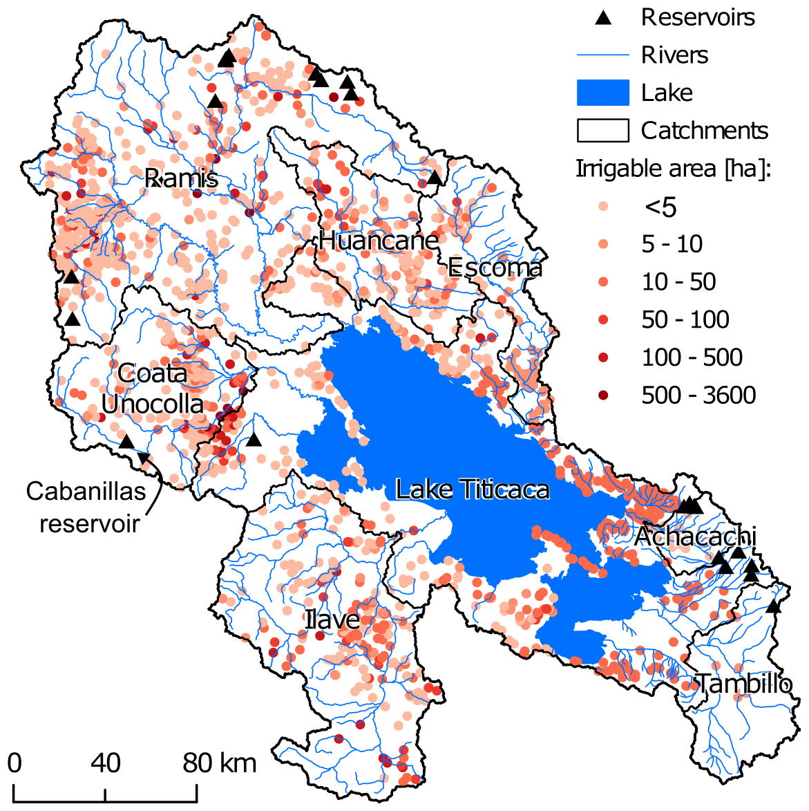
Figure 3Locations of irrigation systems in terms of irrigable area (Ministerio de Medio Ambiente y Agua, 2013; https://snirh.ana.gob.pe, last access: 12 May 2023).
2.5 Glaciological and hydrological control data
2.5.1 Geodetic mass balance of the glaciers
Within the study area, no observations are available at the scale of small glacierized catchments. Only geodetic mass balance data are computed at the scale of the entire Lake Titicaca hydrosystem (e.g., Dussaillant et al., 2019; Hugonnet et al., 2021a). The Hugonnet et al. (2021a) dataset, which is based on ASTER satellite stereo imagery, is available for the period 2000–2019. The mass balance at a 5-year time step is provided for RGI 6.0 glacier outlines. The error range of the Hugonnet et al. (2021a) dataset is smaller than the Dussaillant et al. (2019) dataset, and the interpolation of glacier elevation changes is based on Gaussian process regressions. Therefore, we used the Hugonnet et al. (2021a) dataset.
2.5.2 Streamflow records
Seven streamflow gauges (see Table 1 and Fig. 1) with daily records were used in this study. The gauged (ungauged) area represents 76 % (24 %) of the total area of the catchments that feed the lake. The quality of the Peruvian gauge data can be considered satisfactory since monthly streamflow gauging is performed to calibrate the rating curves, but on the Bolivian side the quality of the Escoma and Achacachi data is questionable. According to SENAMHI–Bolivia, the river stages measured in Escoma and Achacachi are prone to systematic errors due to erroneous measurements made by observers with limited measurement training (Escoma) and/or changes in the geomorphology of the riverbed (Achacachi). Streamflow gauging is only carried out twice in a hydrological year.
2.5.3 Lake water levels
We had access to data recorded at two water level gauges: Puno and Huatajata (see Fig. 1). The Puno gauge (also known as Muelle ENAFER) is managed by SENAMHI–Peru, while the Huatajata gauge is managed by SENAMHI–Bolivia. The daily historical water levels from Puno are more reliable. In the case of Huatajata, inconsistencies were detected in the records made prior to 1998. Additionally, during a field visit, it was observed that the Huatajata measurement scale is prone to displacement. Therefore, in this study we used data from Puno, which provide continuous daily water levels (m a.s.l.) over the period 1982–2016.
3.1 Modeling framework used to quantify the water balance in a high mountain lake hydrosystem
The water balance of Lake Titicaca was modeled at a daily time step for the hydrological period from 1 September 1981 to 31 August 2016 (hereafter 1982–2016) using a lumped model store following the equation
where Plake, Qin, Elake, and Qout are, respectively, direct precipitation over the lake, inflow from upstream catchments, evaporation from the lake, and downstream outflow. The term represents the storage change in the lake over a time window. Qgw represents the net groundwater exchange, and ε represents the error that cannot be explained by the components of the water balance. The unit of the water balance terms is millimeters per day.
WEAP (Yates et al., 2005) was adapted and used to represent the water balance dynamics. The models in WEAP typically seek a compromise between data availability and the complex representation of hydrological processes. This is essential in the context of poorly gauged regions, where it is not possible to represent all hydrological processes in sufficient detail. Unlike the study by Lima-Quispe et al. (2021), which also uses WEAP, this study uses a daily time step and a different approach to simulating irrigation water allocation. We acknowledge that there is an overlap in the precipitation and air temperature data as well as in the irrigable area on the Bolivian side. However, in order to implement the model at a daily time step, it was necessary to collect new data updated to the required timescale. In addition, new data were available, such as lake bathymetry and irrigable area on the Peruvian side. Figure 4 shows the main processes and parameters of the modeling chain used.
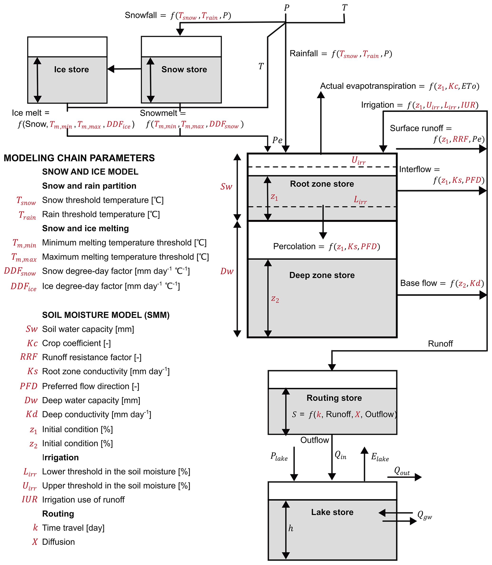
Figure 4Main processes and parameters (in red) of the modeling chain used to simulate the water balance of Lake Titicaca. P, T, ETo, Pe, Plake, Qin, Elake, Qgw, Qout, and h stand for, respectively, precipitation, air temperature, reference evapotranspiration, effective precipitation, direct precipitation over the lake, upstream catchment inflow, evaporation from the lake, net groundwater exchange, downstream outflow, and lake storage. Root zone and deep zone stores were modified based on Yates et al. (2005).
3.1.1 Direct precipitation over the lake
Plake was extracted from GMET for the outline of the lake. The large area and volume of Lake Titicaca favor absorption of solar radiation and result in higher water temperatures than in the surrounding areas, which, in turn, induces convection and higher precipitation over the center of the lake (Roche et al., 1992). However, the magnitude and spatial distribution of precipitation over the lake are not understood well. GMET included two precipitation gauges located on two different islands in the lake. In this study, the extracted data were used directly without correcting for scaling factors. Significant underestimation of precipitation could lead to significant error.
3.1.2 Upstream inflow
Qin was estimated using a conceptual modeling approach that combines a degree-day model for simulating snow and ice processes with the Soil Moisture Model (SMM, part of WEAP) (Yates et al., 2005) to simulate the processes contributing to the generation and regulation of water storage and water flow in the catchments, including irrigation. The model was applied using the same 100 m elevation bands in each catchment to account for snow and ice accumulation and melt, and glacierized and non-glacierized areas were distinguished in each elevation band.
For the snow and ice processes, a degree-day model was applied that considered two stores: one for ice and one for snow (see Fig. 4) in a semi-distributed mode with 100 m elevation bands. However, each glacier in each catchment was simulated separately. For snow accumulation, the liquid (Prain, mm) and solid (Psnow, mm) fractions of total precipitation were estimated from a linear separation between the snow (Ts) and rain (Tl) temperature thresholds according to values (see Table 2) recommended in Ruelland (2023). Potential (maximum) snowmelt was calculated as DDFsnow(T−Tm), where DDFsnow is the degree-day factor (mm d−1 °C−1), T is the air temperature (°C), and Tm is the melting temperature threshold (°C). Tm was calibrated according to two values (Tm,max and Tm,min), where the maximum value occurs in austral summer and the minimum value in winter. In the outer tropical regions, the amplitude of the diurnal range of air temperature is indeed considerable in winter. This means that it is warmer during the daytime, which can increase melting, while cold conditions prevail at night. The seasonal variation of Tm was calculated using the following equation:
where Tm,max and Tm,min are the maximum and minimum temperature thresholds (°C) and D is the Julian day. The maximum value of Tm was assumed to occur on 10 January and the minimum on 12 July.
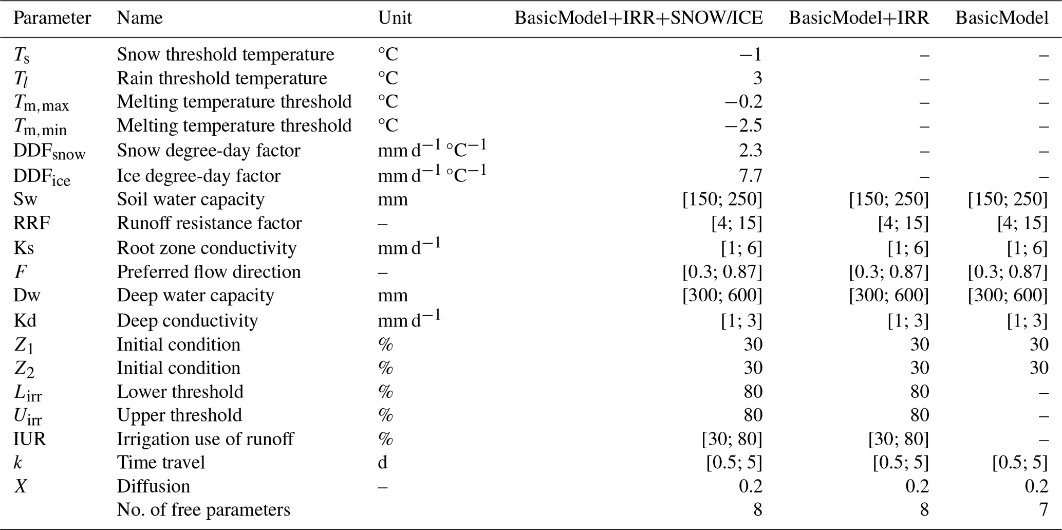
Table 2Parameters of the upstream catchment model of Lake Titicaca and the associated fixed values or ranges tested. The ranges presented were used to generate the random sample of hypercubes in the Monte Carlo approach.
Actual snowmelt (Msnow) was determined as a function of maximum snowmelt and snow accumulation. For ice melt (Mice), the same approach was used as for potential snowmelt, except that DDFsnow was replaced by an ice degree-day factor (DDFice). Ice melts when it is not covered by a snowpack. The daily mass balance (B, mm w.e.) and effective precipitation in glacierized areas (Peg, mm w.e.) in each elevation band (j) were computed as follows:
The annual mass balance in each evaluation band, Ba,j, was estimated as the sum of the daily mass balance in a hydrological year. The annual mass balance was also calculated for individual glaciers (Ba,g) for comparison with the available glaciological and geodetic mass balance. Ba,g was calculated as
where Ag,j and Ag are the glacier area in the elevation band j and the total glacier area, respectively.
The glacierized surface area (RGI Consortium, 2017) was fixed for the period simulated. The area provided for the year 2000 was considered an intermediate value for the period 1982–2016. Ice thickness was also assumed to be infinite. The air temperature in each elevation band (Tj) was estimated as ), where TGMET,j is the air temperature derived from GMET for each elevation band, ZGMET is the mean areal elevation signal from GMET in the elevation band j, Zj is the mean elevation of the elevation band, and Γ is a constant temperature lapse rate that was set to the value calculated from GMET (i.e., 5.8°C km−1). The precipitation extracted from GMET for each elevation band was used directly with no modification.
Regarding SMM, it is a one-dimensional model based on two stores (see Fig. 4). The first store represents the root zone and the second the deep zone (Yates et al., 2005). The model without irrigation has seven free parameters as shown in Fig. 4, of which the crop coefficient (Kc) can be set using reference values from the literature. In addition, there are two parameters associated with the initial states of the two stores called z1 and z2. An additional parameter was included for runoff routing using the Muskingum equation. SMM is driven by precipitation and reference evapotranspiration estimated by the modified Penman–Monteith method (Maidment, 1993) for a grass crop 0.12 m in height and with a surface resistance of 69 s m−1. The climate input data are detailed in Sect. 2.2. The effective precipitation in the elevation band j of both the non-glacierized and glacierized fractions is given as
where Prain,ng and Msnow,ng refer to rainfall and snowmelt in the non-glacierized fraction (mm). The term Ang is the relative area of the non-glacierized fraction.
In SMM, water requirements (WRs) for irrigation are determined by crop evapotranspiration (from seasonal crop coefficients (Kc) and reference evapotranspiration) and the depletion of available water in the root zone store (see Fig. 4). Kc adjusts the reference evapotranspiration to reflect crop-specific characteristics (Allen et al., 1998), such as phenology. It was derived using cropping calendar and crop type data (Autoridad Nacional del Agua, 2009, 2010; Instituto Nacional de Estadística, 2015). The lower and upper irrigation threshold parameters (Lirr and Uirr; see Table 2 and Fig. 4) dictate both the timing and quantity of water used for irrigation (Yates et al., 2005). When the relative soil moisture of the root zone store drops below the lower threshold, a water requirement is triggered and irrigation is supposed to be applied up to the upper threshold (Yates et al., 2005). The irrigation use of runoff (IUR) method was used to allocate water. This method consists of setting or calibrating a percentage (IUR) of a catchment's runoff (before the runoff reaches the main river) that can be used for internal irrigation. IUR focuses on water allocation at the catchment scale, especially when hundreds of irrigation systems are to be represented together. Simulating each of the irrigation systems shown in Fig. 3 individually would not be feasible at the scale of this study, and the IUR approach is thus better suited for this. The irrigation net consumption, IRRnet, was calculated as
where Qwi is runoff without irrigation (mm), IUR is a calibration parameter expressed as a percentage, WR is the irrigation water requirement (mm), and IRRrf is the irrigation runoff fraction expressed as a percentage. The term is the water withdrawn for irrigation. IRRrf is calculated as follows: (i) in the first iteration, SMM simulates Qwi; (ii) in the second iteration, runoff is simulated assuming that the full WR is supplied; and, (iii) finally, IRRrf is estimated based on how much runoff would flow due to irrigation alone.
3.1.3 Evaporation from the lake
Elake was estimated using the Penman method for open water (Penman, 1948). This method is justified because it requires fewer data than an energy balance approach but is not as simple as a temperature-based approach. The Penman method also attempts to incorporate the energy balance in a simplified manner and includes mass transfer. The equation is given as
where Elake is the evaporation (mm d−1), Δ is the slope of the vapor pressure curve (kPa °C−1), λ is the latent heat vaporization set at 2.45 MJ kg−1, and γ is the psychrometric constant (kPa °C−1). The terms Rn and G are net radiation at the water surface and heat storage changes (MJ m−2 d−1), respectively. f(U2) is the function of wind speed measured at 2 m above the lake surface that is equal to c(a+bU2), where the constants a=10, b=5.4, and c=0.26 for Lake Titicaca were taken from Delclaux et al. (2007). Also, es is the vapor pressure at the evaporating surface (kPa), and ea is the vapor pressure at 2 m above the lake surface (kPa). Δ is given as , where Tw and T are the evaporating surface temperature and air temperature (°C), respectively.
Rn is the sum of net shortwave radiation (K) and net longwave radiation (L). K is given as Kin(1−α), where Kin is the incident solar radiation (MJ m−2 d−1) and α is the albedo of the water surface. The L component is the difference between the incident flux (Lin) emitted by the atmosphere and clouds and outgoing radiation (Lout) from the evaporating surface. Lin and Lout can be estimated with Eqs. (9) and (10), respectively. For Lin, we used the equation calibrated by Sicart et al. (2010) on the Zongo glacier, which is located at a distance of about 100 km from Lake Titicaca. The authors suggest that the calibration can be used in the tropical Andes.
where, for a daily time step, C is equal to 1.24; ea is the vapor pressure (hPa); σ is the Stefan–Boltzmann constant (set at MJ m−2 K−4 d−1); τatm is the atmospheric transmissivity (–) that can be approximated as ; Sextra is the theoretical shortwave irradiance (MJ m−2 d−1) at the top of the atmosphere; and εw is the water emissivity set at 0.98 (–).
The term G (heat storage change) in Eq. (8) was estimated using the approach and assumptions of the study conducted by Pillco Zolá et al. (2019) on Lake Titicaca.
where cw is the specific heat of water ( MJ kg−1 °C−1), ρw is the water density (1000 kg m−3), Vmix is the volume above the mixing depth (m3), and Alake is the surface area of the lake (m2). d is the change in water temperature (°C) over the time interval (d).
Air temperature was obtained from GMET, while all the other meteorological variables were obtained from ERA5-Land (Sect. 2.2). Since there are no long-term measurements of lake surface water temperature (LSWT) and the remotely sensed datasets do not cover the entire study period, the Air2Water model (Piccolroaz et al., 2013; Toffolon et al., 2014) was used to simulate LSWT. Calibration and evaluation were performed against ARC-Lake V3 remotely sensed data (MacCallum and Merchant, 2012) (see Appendix B).
3.1.4 Downstream outflow
Qout was simulated using the rating curve shown in Fig. 5a. This curve was established 30 years ago based on a hydrodynamic simulation of the Desaguadero River (INTECSA et al., 1993b). The elevation corresponds to the vertical datum of Peru. The rating curve was used for the entire study period and implemented in the model in combination with the lake bathymetry (see Fig. 5b) carried out between 2016 and 2019 by ALT.
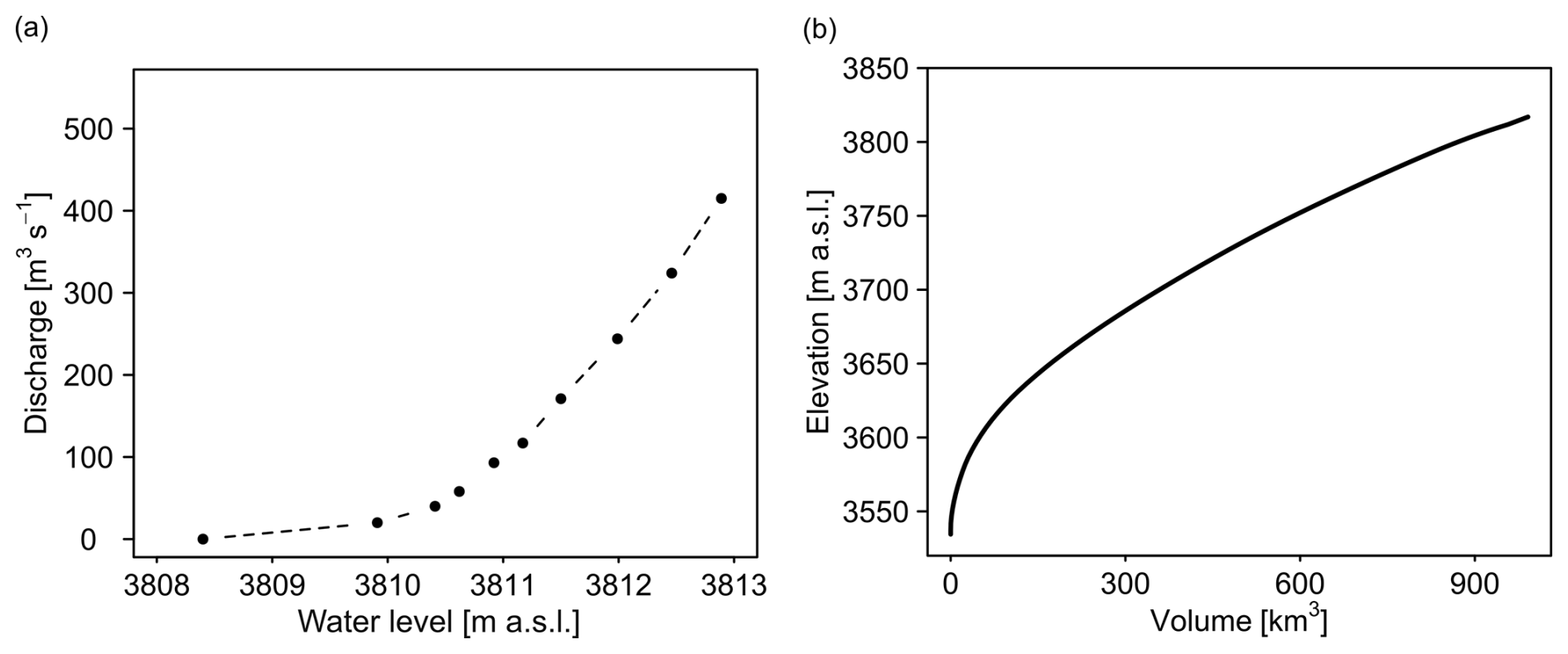
Figure 5Information used to simulate Qout for (a) the rating curve and (b) the bathymetry. The rating curve of the lake outlet to the Desaguadero River was obtained from the master plan (INTECSA et al., 1993b). In both figures the elevation is referenced to the Peruvian vertical datum. The bathymetry (i.e., the relationship between lake water level and storage volume) was recorded by ALT between 2016 and 2019.
3.1.5 Storage change
was calculated directly from the water levels measured at the Puno gauge. Storage change is basically the difference between the water levels of the current time step and the previous time step.
3.1.6 Net groundwater exchange
Qgw was considered negligible. According to INTECSA et al. (1993a), the leakage from Lake Titicaca to the aquifers is very limited, and the lake can be considered an almost completely closed surface system. This is because the lake bed is composed of sediments with very low permeability. In this case, the only areas of high permeability would be limited to alluvial deposits saturated by water that mostly flows towards the lake. According to the same study, the inputs from alluvial deposits were 0.56 m3 s−1. Therefore, omitting Qgw from the water balance is justified.
3.2 Evaluation of the modeling framework
The performance of the lake water balance model was evaluated using both the error term of Eq. (1) and the RMSE computed between observed and simulated water levels. Since the Qin and Elake were modeled, intermediate calibration and evaluation were necessary. Evaporation measurements are not available in the study area to evaluate the performance of the Elake. Therefore, a formal calibration and evaluation procedure was only implemented for the Qin estimates. The procedure was applied sequentially, first to obtain the model parameters simulating snow and ice processes (see Appendix C) and then to calibrate and evaluate the upstream catchment model using the Nash–Sutcliffe efficiency index (Nash and Sutcliffe, 1970) calculated on the root-mean-square-transformed streamflow (NSEsqrt) in order to provide an intermediate fit between high and low flows (Oudin et al., 2006).
3.2.1 Upstream catchment model
The upstream catchment model shown in Fig. 4 has 15 parameters. However, seven of the parameters were set to reduce the number of free parameters. Four parameters (Tm,max, Tm,min, DDFsnow, and DDFice) related to snow and ice store were set to values obtained in the Zongo catchment (see Appendix C). The simulated mass balance of all glaciers of the Titicaca hydrosystem was compared with the geodetic mass balance (Hugonnet et al., 2021a) for the period 2000–2009. Similarly, two parameters of the irrigation module, Lirr and Uirr, were set to 80 %. Winter et al. (2017) used a threshold of 100 % for furrow irrigation in California. However, a value of 80 % is reasonable for our study area because it is irrigated under conditions of limited water availability. X (routing store) was set to a default value (0.2) in WEAP. A total of eight free parameters were kept, as shown in Table 2. The procedure used to obtain the set of parameters with the best performance and the subsequent evaluation consisted of four steps.
First (Step 1 in Fig. 6), the model was run for the period 1980–2016 (of which the first 2 years were used as a warmup period) with 10 000 parameter sets generated from a random sample of hypercubes from the Monte Carlo approach within the parameter intervals tested (see Table 2). Second (Step 2 in Fig. 6), the best-performing parameter sets in terms of NSEsqrt were identified along with subperiods consisting of (i) 5 continuous years (i.e., seven subperiods between 1982 and 2016) and (ii) 5 discontinuous years identified as coldest, warmest, driest, and wettest (i.e., four discontinuous subperiods between 1982 and 2016). The 11 best-performing parameter sets were selected using different subperiods. Third (Step 3 in Fig. 6), the mean of 11 streamflow simulations generated with the selected parameter sets was calculated. Fourth (Step 4 in Fig. 6), the performance of the mean of the streamflow simulations over the 11 subperiods was evaluated using the NSEsqrt criterion.
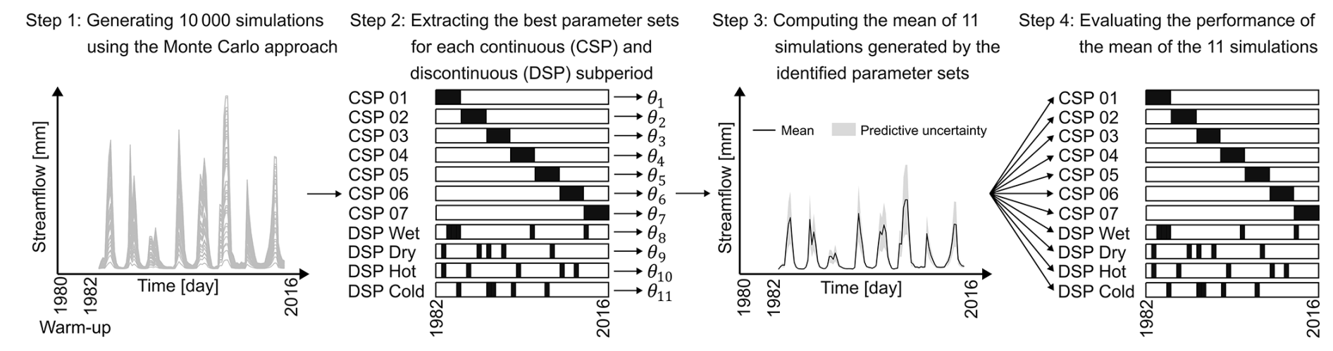
Figure 6Procedure used to evaluate the upstream catchment model to estimate the Qin in each gauged catchment.
Two objectives justify the use of seven continuous and four discontinuous subperiods. The first objective was to evaluate the transferability of the model parameters to nonstationary conditions within the period 1982–2016, including particularly contrasted subperiods in terms of precipitation and temperature. In addition, continuous subperiods were suitable for assessing the transferability of the water allocation parameter (IUR). If there had been a significant and sustained increase in the irrigation withdrawals, the IUR parameter would not have been transferable over time and would therefore have varied over the period 1982–2016. However, it is important to note that irrigable area, crop type, and Kc remain under the assumption of stationarity. The second objective was to consider the parameterization uncertainty through uncertainty envelopes and confidence intervals in the simulations resulting from the 11 parameter sets used over the whole 1982–2016 period.
3.2.2 Sensitivity assessment of model predictability to irrigation and snow and ice processes
To evaluate the sensitivity of the modeling chain to net irrigation consumption and snow and ice processes, different processes were progressively excluded from the modeling structure. Three model structures were tested in the following configuration: (i) BasicModel+IRR+SNOW/ICE, which represents the full reference model structure (as shown in Fig. 4); (ii) BasicModel+IRR, where the processes associated with snow and ice (accumulation and ablation) are excluded but irrigation is maintained; and (iii) BasicModel, where snow and ice processes and irrigation consumption are excluded. The objective was to evaluate whether a simpler structure in terms of the hydrological processes considered performed better or worse than a more complex structure in simulations of catchment streamflow and lake water levels. This is justified because, a priori, snowfall and the proportion of glacierized area and irrigable area are very limited in the catchments that contribute to the lake (see Table 1), and their impact on the streamflow and water level prediction may be negligible. In addition, the data used to represent and control these processes are very limited, which can lead to inaccuracies that could worsen the simulations of streamflow and lake water levels instead of improving them. Table 2 shows the active and inactive parameters in the three model structures.
3.2.3 Transferring parameters to the ungauged catchments
The approach used to transfer the parameters to the ungauged catchments consisted of the following steps: (i) the median of the parameter sets obtained for the seven gauged catchments was calculated for each subperiod, thus generating 11 parameter sets; (ii) the upstream catchment model was run for the 11 parameter sets; and (iii) the mean of the 11 streamflow simulations was calculated, including the confidence interval.
4.1 Modeling chain performance
4.1.1 Performance of the geodetic mass balance simulated by the model for Titicaca glaciers
Figure 7 shows the comparison between the simulated and geodetic mass balances. The scatterplots reveal significant variability in model performance, with some glaciers (represented by each point) close to the identity line and others deviating significantly. The model simulates a more negative glacier mass balance compared to the geodetic glacier mass balance. Figure 7a displays glaciers according to their surface area, while Fig. 7b shows them based on their mean elevation. The model performed more effectively in the catchments that concentrate 92 % of the glacierized area (Achacachi, ungauged catchments, Tambillo, and Escoma). The model performed very poorly in Ramis (see Table 3), but the proportion of glacierized area in that catchment is very small (0.1 %). Therefore, the proportion is expected to have a limited impact on streamflow predictions. Additionally, the model performs much better in the case of large glaciers than small glaciers (see Table 3). For example, for large glaciers representing 84 % of the glacierized area, the weighted simulated mass balance for all the catchments has a bias of 11 %, which is within the error range of the geodetic mass balance (see Table 3). Much more obvious is the dependence on elevation (see Fig. 7b). The model performed very poorly on glaciers with mean elevations below 5100 m a.s.l., which represent only 10 % of the simulated glaciers. At elevations above 5200 m a.s.l., i.e., 68 % of the glaciers, the points are distributed around the identity line. The notable variability in model performance (see Fig. 7b) could be attributed to inaccuracies in precipitation data for some catchments, as estimating precipitation in high-elevation remote areas remains a complex challenge (Ruelland, 2020). At the catchment scale, the underestimation and overestimation of glacier-wide mass balance are compensated for, and the biases are relatively small (see Table 3).
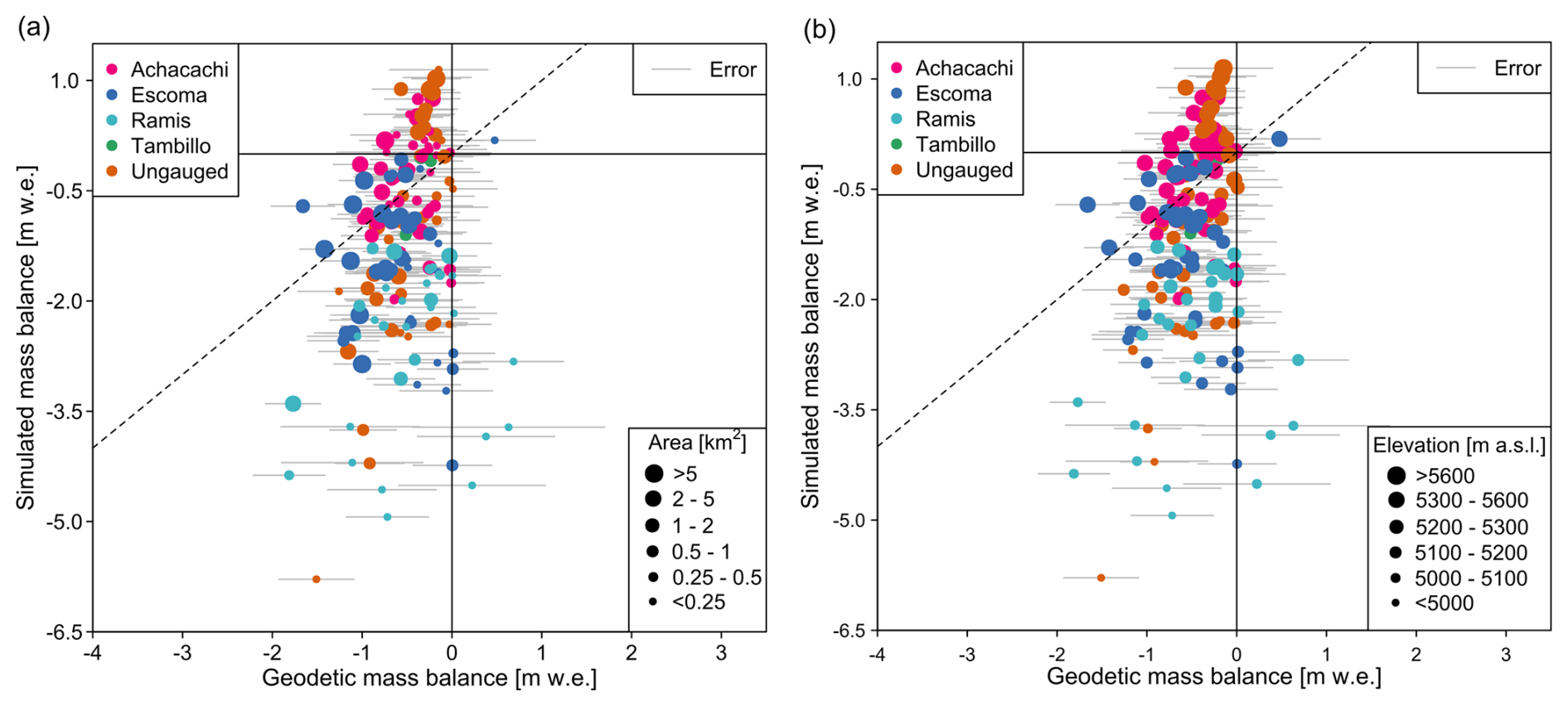
Figure 7Scatterplots comparing simulated and geodetic glacier mass balances for 2000–2009, based on the remotely sensed observation of Hugonnet et al. (2021a). The dot size represents the (a) glacier area and (b) mean elevation. The dashed line indicates the identity line, while the gray line represents the error in the geodetic glacier mass balance.
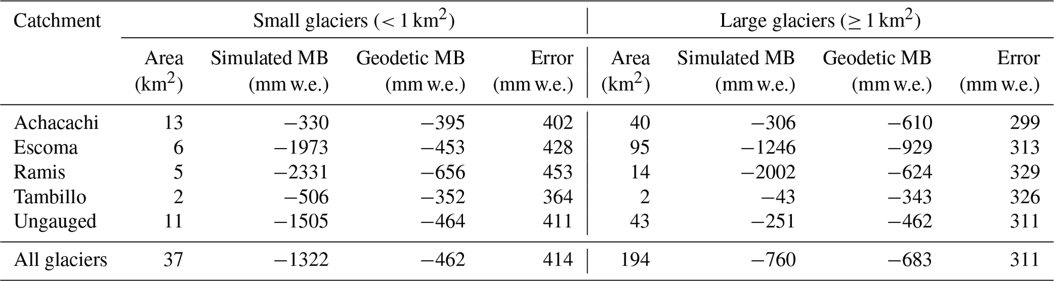
Table 3Comparison of simulated and geodetic glacier mass balances (MBs) in upstream catchments for the period 2000–2009. The catchment-scale mass balance was calculated as an area-weighted average of each glacier. The error corresponds to the geodetic glacier mass balance and was calculated as a weighted average for each catchment.
4.1.2 Performance and sensitivity of the upstream catchment model to irrigation and snow and ice processes
Figure 8 shows the distribution of the performance of the three modeling options (BasicModel+IRR+SNOW/ICE, BasicModel+IRR, and BasicModel) in the evaluation made for each catchment. A striking feature is that the performance in the catchments on the Peruvian side (Ramis, Ilave, Coata Unocolla, and Huancane) was significantly better than in the catchments on the Bolivian side (Escoma, Tambillo, and Achacachi). The performance of the three models is distributed symmetrically in the boxplots in each catchment. This suggests that there are no significant performance differences between the three models. Therefore, Qin is not very sensitive to net irrigation consumption or snow and ice processes. This reflects the fact that the upstream catchments of Lake Titicaca are dominated by a pluvial monsoonal climate regime and that contributions from glacierized areas and snow have little influence on the Qin prediction. However, in terms of mean and median NSEsqrt, BasicModel+IRR+SNOW/ICE and BasicModel+IRR generally performed slightly better than BasicModel, but the differences are marginal: in most cases the difference is between 1 % and 3 %. However, in Achacachi, the NSEsqrt obtained with BasicModel+IRR+SNOW/ICE is 6 % higher than the value obtained with the BasicModel+IRR and BasicModel models.
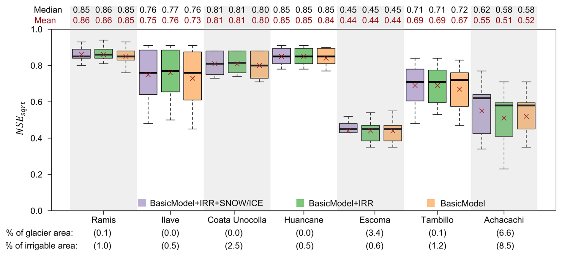
Figure 8Performance distributions of the three modeling options (BasicModel+IRR+SNOW/ICE, BasicModel+IRR, and BasicModel) in each gauged catchment in the evaluation. The size of the sample in each boxplot is 11 (resulting from the procedure presented in Fig. 6).
4.1.3 Performance of the modeling chain with respect to lake water levels
Figure 9 shows the simulation of daily water levels in Lake Titicaca over the 1982–2016 period. Three different estimates of Qin were used, one from BasicModel+IRR+SNOW/ICE, one from BasicModel+IRR, and one from BasicModel. The results show that the models are able to simulate the amplitude and frequency of annual, interannual, and decadal water level fluctuations reasonably well. Visually, the performances of the three Qin estimates appear to be relatively similar. Based on the ε term, BasicModel+IRR performed better than BasicModel+IRR+SNOW/ICE and BasicModel. The difference in the ε term between BasicModel+IRR+SNOW/ICE and BasicModel+IRR was 0.01 mm. When snow and ice processes and net irrigation consumption were excluded, the error increased by 0.03 mm d−1. However, the differences in the error were marginal. Figure 9 shows that, in the mostly dry years of the 1990s, BasicModel+IRR+SNOW/ICE and BasicModel+IRR simulated daily water levels better. However, the performance measured by the RMSE differed in the error term. In that case, BasicModel performed best. This is because the RMSE was calculated using daily water level data (cumulative change in storage over time), whereas the ε term was computed directly from the water balance at each time step. Inaccuracies in some time steps were then propagated to later time steps due to the slow response of the lake. The RMSE obtained was very small compared to the average water level (3809.7 m a.s.l.).
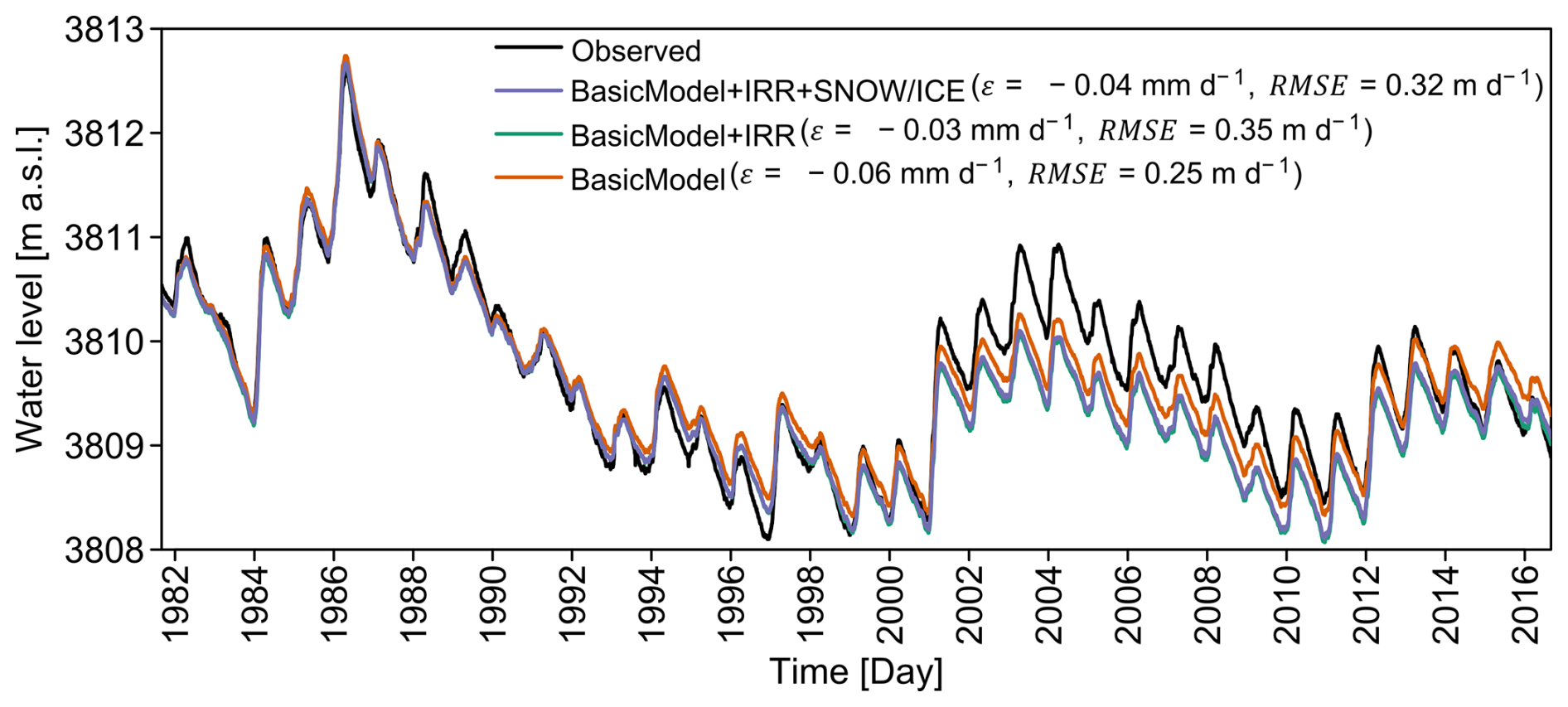
Figure 9Performance of the modeling chain compared with the water levels of Lake Titicaca measured in Puno. Modeling was evaluated using the error (ε) term of the lake water balance and RMSE. Three simulations of water levels are presented because the models produced three different estimates of Qin.
A striking feature of Fig. 9 is the systematic underestimation of daily water levels between 2001 and 2010. This is related to inaccuracies in the estimation of water balance terms. The hydrological response of Lake Titicaca is relatively slow, and it was possible to verify that significant errors were present between 2001 and 2004 but were not underestimated over the whole decade (2001–2010) (see Fig. D1). In 2001, the outflow gate to regulate outflows into the Desaguadero River was completed, and dredging of the Desaguadero River began. This could mean fewer outflows into the Desaguadero River and consequently more storage in the lake. However, even assuming that there were no downstream outflows in those years would not compensate for the underestimation. Looking for other sources of error, discussions with ALT revealed that the lake sometimes received inflows from the Desaguadero River, especially in wet years. This could be the case, since 2001 and 2004 were wet hydrological years, but other than verbal communication there are no records to support such a claim.
BasicModel+IRR+SNOW/ICE produced a reasonably realistic simulation with an even smaller error, with marginal differences, than BasicModel. Consequently, BasicModel+IRR+SNOW/ICE can be considered a reference structure for providing an estimate of the water balance of the Lake Titicaca hydrosystem.
4.2 Simulated water balance
4.2.1 Simulated water balance in upstream catchments
Table 4 shows the mean annual water balance for the hydrological period 1982–2016 simulated by BasicModel+IRR+SNOW/ICE. Some terms (AEni, IRR, and Qin) were calculated as the average of 11 ensemble members. At the scale of all the upstream catchments (see Table 4), the annual precipitation is 723 mm, of which 6 % is estimated to be snowfall. Thus, despite the elevations at which the study area is located (> 3810 m a.s.l.), the precipitation regime is clearly dominated by rainfall. This regime has a unimodal pattern with a strong seasonal cycle between the rainy and dry seasons (see Fig. 10). This is very characteristic of the outer tropical areas, where precipitation mainly occurs in the summer and the dry season in winter. In the upstream catchments, snowmelt accounts for 6 % of the total input (). Snow remains on the ground for only a very short time, as there is practically no time lag between snowfall and snowmelt (see Fig. 10). Snowfall and snowmelt have a less accentuated seasonal cycle, as the rare precipitation that occurs in the dry season is mostly snow. The contribution of ice melt was simulated to be 6 mm yr−1 on average, which represents only 1 % of the total input in upstream catchments. However, the contribution of ice melt is slightly higher in the Achacachi and Escoma catchments, where the simulated value is 7 %. Most ice melt occurs between October and November (see Fig. 10) because the temperature is above the melting threshold and glaciers are mostly free of snow cover. Δice is negative, indicating a loss in ice stock.
Table 4Mean annual water balance (mm) in the upstream catchments for the hydrological period 1982–2016 simulated with BasicModel+IRR+SNOW/ICE. P, Prain, Psnow, Msnow, Mice, AEni, IRR, Δice, Δsnow, ΔSM, and Qin represent total precipitation, rainfall, snowfall, snowmelt, ice melt, actual evapotranspiration in non-irrigated areas, net consumption of irrigation water, variation in ice storage, variation in snow storage, variation in soil moisture storage, and streamflow in upstream catchments, respectively. The water balance follows the equation .
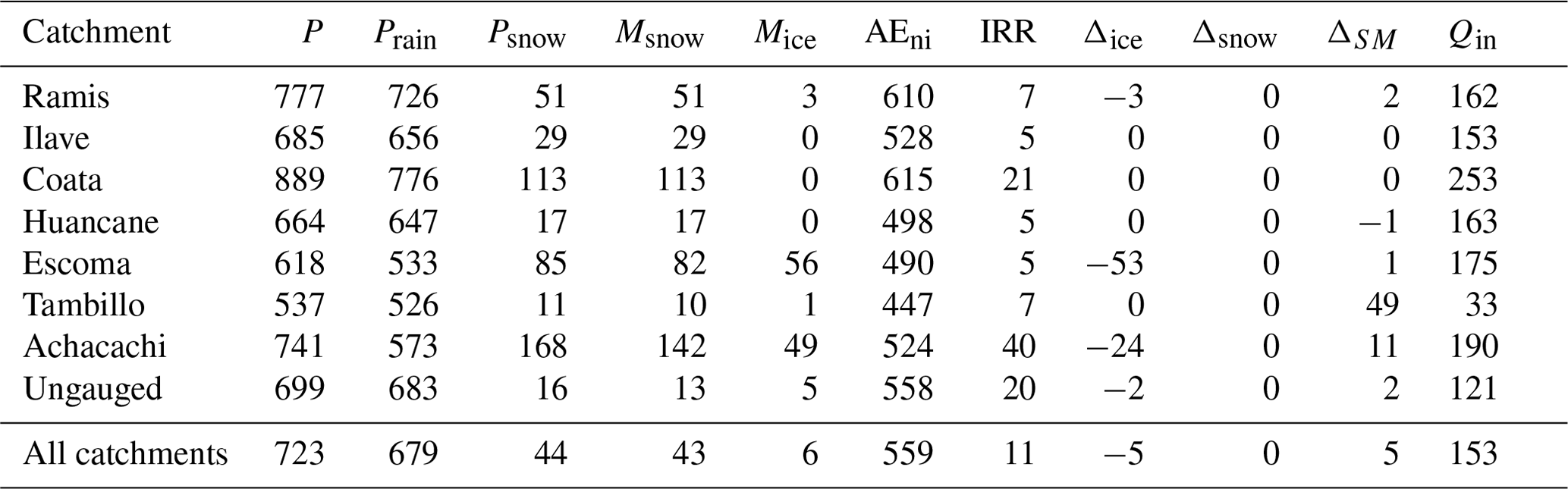
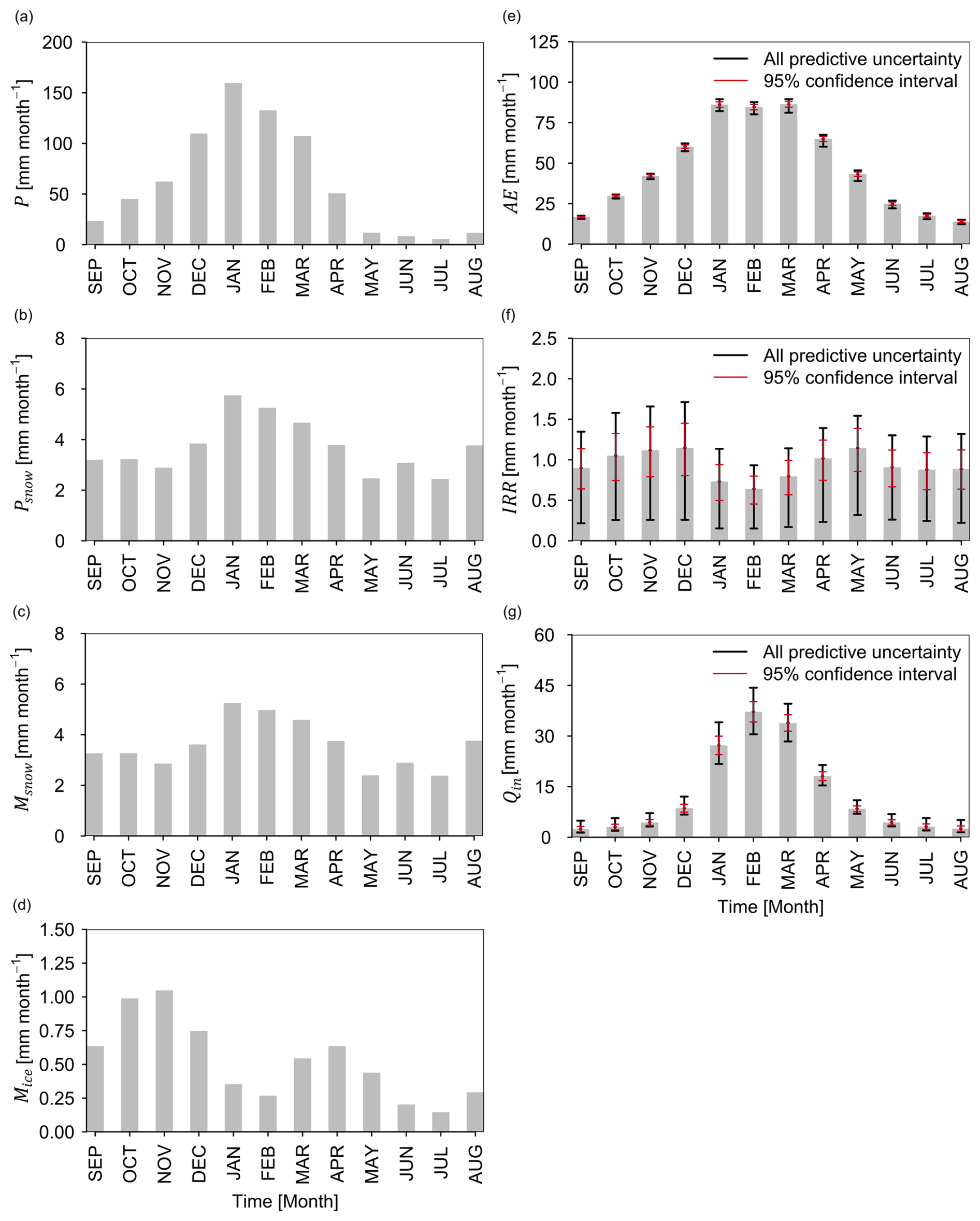
Figure 10Seasonal cycle (monthly average for the period 1982–2016) of the water balance in the upstream catchments of Lake Titicaca simulated with BasicModel+IRR+SNOW/ICE. P, Psnow, Msnow, Mice, AE, IRR, and Qin represent total precipitation, snowfall, snowmelt, ice melt, actual evapotranspiration, irrigation net water consumption, and streamflow in the upstream catchments. For some terms (AE, IRR, and Qin), the gray bars were estimated as the mean of the 11 ensemble members resulting from the procedure shown in Fig. 6. The predictive uncertainty is presented for both the entire prediction range (i.e., all predictive uncertainty) and the 95 % confidence interval. “All predictive uncertainty” was estimated as the maximum and minimum values of the ensemble members. The terms associated with snow and ice are not subject to predictive uncertainty because fixed parameters were used (see Table 2).
Annual actual evapotranspiration (AE) was simulated at 570 mm, of which 2 % corresponds to net irrigation water consumption (IRR). AE is highest between January and March and lowest between July and September (see Fig. 10). IRR is concentrated in the transition season (see Fig. 10). The simulated streamflow is about 153 mm, which represents 21 % of the total outflow in upstream catchments (AE+Qin), the remaining 79 % being actual evapotranspiration. IRR represents 7 % of Qin. The seasonal cycle of Qin shows that the peak is in February, while Qin is low from June to November. The predictive uncertainty associated with the upstream catchment model parameters is shown in Fig. 10 for the terms AE, IRR, and Qin. The prediction range of AE is very narrow (see Fig. 10) compared to that of IRR and Qin, indicating that evapotranspiration is less sensitive to the model parameters. The range of prediction of IRR is quite wide (see Fig. 10), indicating that the simulations are very sensitive to SMM parameters. The range of the prediction of Qin is also wide (see Fig. 10). However, the average predictions fitted the measured streamflow and model performance reasonably well (see Fig. 8).
4.2.2 Simulated water balance in the lake
Figure 11a shows the annual evolution of the water balance, and Table 5 shows the long-term average values. Over the period 1982–2016, the average annual precipitation over the lake was 744 mm (σ=144 mm) and the inflow from the upstream catchments 958 mm (σ= 392 mm). This means that 44 % of the inflows come from direct precipitation over the lake, while the remaining portion (56 %) comes from upstream catchments. Regarding outflows, the annual evaporation from the lake is 1616 mm (σ= 28 mm) and the downstream outflow is 121 mm (σ= 191 mm). Thus, 93 % of the losses are due to evaporation and 7 % due to downstream outflow. The measured storage change for the period 1982–2016 was −50 mm, indicating a drop in the water level. The simulated change in storage was −35 mm, which indicates an overestimation. Therefore, the water balance closure has an error of about −15 mm. Compared to evaporation, Plake and Qin showed significant interannual variability (see Fig. 11a). Elake was subject to less pronounced interannual variability but showed an increasing trend over the period 1982–2016 due to the increase in temperature (about +0.1 °C per decade). This means that the interannual variability of water levels depends to a large extent on variations in precipitation over the lake and in the upstream catchments. The highest values of both Plake and Qin occurred between 1985 and 1986 and caused large floods around the lake and in the Desaguadero River, where discharges reached about 900 mm yr−1. In the 1990s, inflows were lowest in the period studied, resulting in a mostly negative change in storage. Substantial inflows to the lake in the early 2000s led to a significant positive change in storage, although this was followed by another dry period that lasted until 2012.
Table 5Lake Titicaca water balance components simulated for the period 1982–2016. The lake water balance follows the equation .
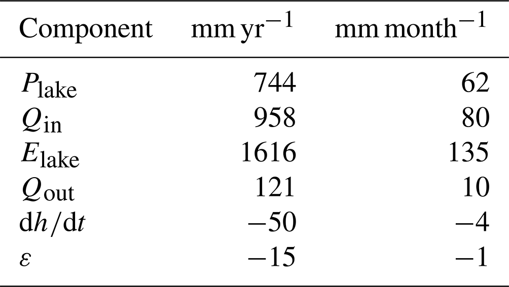
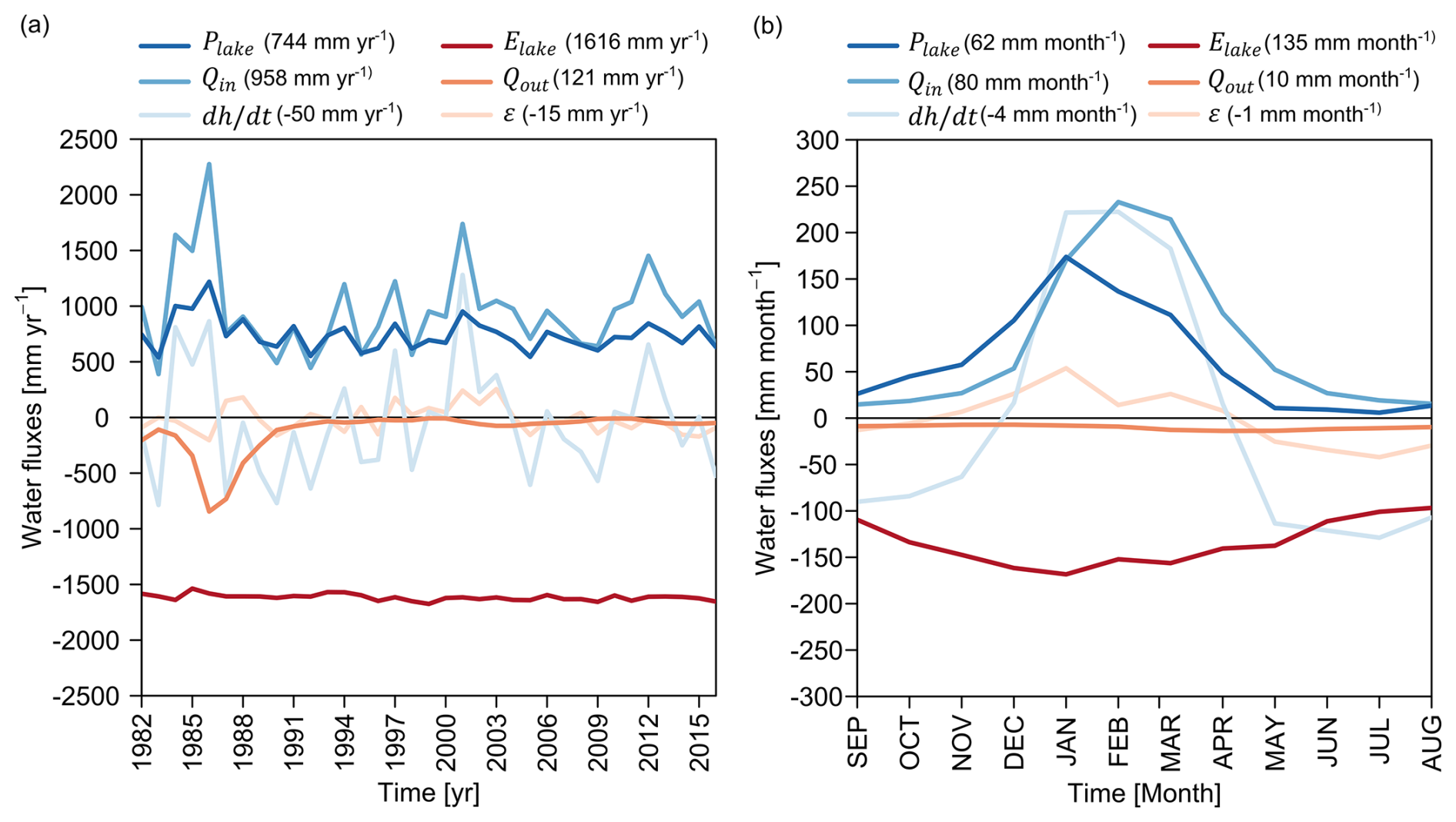
Figure 11Water balance of Lake Titicaca for the period 1982–2016 in terms of (a) interannual variability and (b) seasonal cycle. The values in parentheses correspond to the mean annual or monthly values for the period 1982–2016. The lake water balance follows the equation .
Figure 11b shows a very marked seasonal cycle for precipitation and upstream inflow. For example, the monthly peak in upstream inflow is about 230 mm (in February), while in the dry season the values are very close to 15 mm (in September). One of the features is the lag of upstream inflow with respect to direct precipitation over the lake, which is evidence of the relatively slow hydrological response in the upstream catchments because of the size of the catchment area. The seasonal cycle of evaporation is less marked than that of precipitation and upstream inflow. Although air temperature shows strong seasonality, evaporation is also influenced by other meteorological variables, and heat storage plays a critical role in the seasonal cycle. The peak of the mean monthly evaporation is around 170 mm (in January), while the minimum value is around 95 mm (in August). In Fig. 11b, it is also interesting to observe the seasonal cycle of the error term, which is mostly positive in the rainy season and mostly negative in the dry season. This could indicate that the lake receives net groundwater inflow during the rainy season and is subject to net outflow during the dry season. However, the magnitudes cannot be attributed directly to net groundwater flow because the error term includes both the uncertainty associated with estimating the other terms of the water balance (Plake, Qin, Elake, and Qout) and assumptions concerning the groundwater flow.
5.1 Main findings
This study presents three main novelties. First, our integrated modeling framework accurately simulates the daily water balance of Lake Titicaca without requiring scaling factors. Consequently, the propagation of uncertainty in estimating components of the water balance is significantly reduced. For instance, Fig. 12 illustrates how omitting the calibrated precipitation scaling factor used by Lima-Quispe et al. (2021) leads to unrealistic simulations of lake water levels. Our modeling approach also benefits from (i) a rigorous calibration and evaluation procedure for simulating upstream inflows (see Fig. 6), (ii) the estimation of evaporation from the lake using the Penman method while accounting for LSWT and heat storage, and (iii) estimates of reference evapotranspiration and lake evaporation that account for climate variability, using the ERA5-Land dataset for humidity, wind speed, and solar radiation. This study provides a realistic water balance that estimates most hydrological processes (see Tables 4 and 5), although the role of groundwater remains a major unknown. Its magnitude is expected to be a small component of the total water balance.
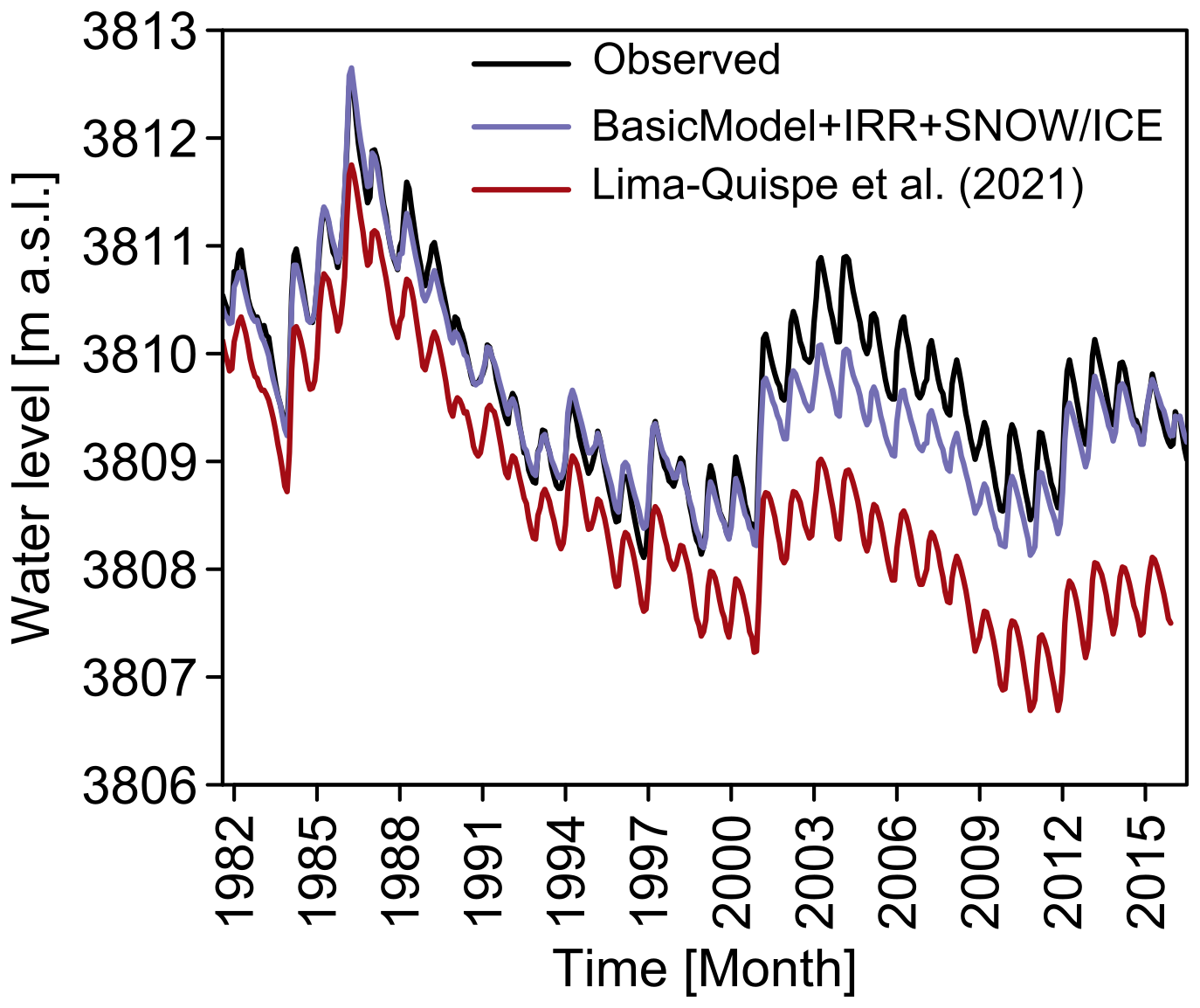
Figure 12Comparison of simulated water levels by BasicModel+IRR+SNOW/ICE (aggregated to the monthly time step) with those obtained by Lima-Quispe et al. (2021) without applying the scaling factor to precipitation over the lake.
Second, through the hydrological sensitivity analysis, we demonstrate that net irrigation withdrawals and snowmelt and ice melt have a minimal impact on lake level fluctuations, indicating that this is primarily driven by rainfall and evaporation variability. However, this does not diminish the importance of glaciers. In fact, glaciers are significant at the scale of the headwater catchments, particularly for supplying water to large cities such as El Alto and La Paz (Buytaert et al., 2017; Soruco et al., 2015), maintaining wetlands like the bofedales (Herrera et al., 2015), and supporting irrigation (Buytaert et al., 2017). In most gauged catchments, incorporating irrigation resulted in only slight improvements in modeling performance. Nonetheless, this approach made it possible to estimate the net consumption due to irrigation at the scale of the catchments that contribute to the lake. Although this consumption is currently low, it is expected to increase significantly due the climatic and anthropogenic changes in the study area. It should also be noted that this process was based not only on soil water deficit, but also on local knowledge of farmers' water allocation practices.
Third, we disentangle the role of the change in heat storage in estimating Elake. Annual evaporation (1616 mm yr−1) is comparable to the evaporation (∼ 1600) of other low-latitude lakes (Wang et al., 2018) and aligns with previous studies of Lake Titicaca (∼ 1600 mm yr−1) (Delclaux et al., 2007; Pillco Zolá et al., 2019). Despite the low air temperature over Lake Titicaca due to its high altitude, the evaporation rate is quite high. This is largely due to net radiation, although humidity, wind speed, and changes in heat storage also play a significant role in the seasonal variation. Regarding heat storage changes, the lake reaches maximum heat gain in October and maximum heat loss in May (see Fig. 13a). Neglecting changes in heat storage leads to overestimation of evaporation during the lake's heating period and underestimation of evaporation during the cooling period (see Fig. 13b). A similar finding was reported by Bai and Wang (2023) for Lake Taihu in China. Although several studies have investigated evaporation from Lake Titicaca using various methods (Carmouze, 1992; Delclaux et al., 2007; Pillco Zolá et al., 2019), our estimates are innovative because they are based on long-term data, including recent periods. Additionally, the accuracy of our estimates was underpinned by a water balance with a small error term, which enhances the reliability of our findings.
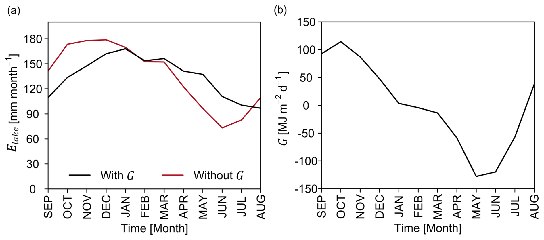
Figure 13(a) Seasonal variations in heat storage and (b) the role of heat storage in the seasonal variation of evaporation from the lake. The figures are based on long-term (1982–2016) average values.
The periods of rising and falling water levels are closely linked to direct precipitation over the lake and upstream inflows (see Fig. 11a), which is mostly influenced by interannual precipitation variability. Understanding the effects of climate oscillations on precipitation variability is therefore crucial for understanding water level changes. Some authors (e.g., Garreaud and Aceituno, 2001; Jonaitis et al., 2021) noted that the interannual variability of precipitation in the region is mainly driven by the El Niño–Southern Oscillation (ENSO). During its warm phase, conditions are typically dry, while during the cold phase conditions are usually wet, although this relationship is not always consistent (Garreaud et al., 2003). For instance, Jonaitis et al. (2021) observed negative precipitation anomalies during La Niña phases and positive precipitation anomalies during El Niño phases in the Lake Titicaca region, though these anomalies were not statistically significant. Segura et al. (2016) argued that El Niño plays an important role in interannual precipitation variability and that decadal and interdecadal variations are influenced by sea surface temperature (SST) anomalies in the central–western Pacific. Therefore, variations in water levels cannot be attributed to ENSO alone. Sulca et al. (2024) found that interannual variations in water levels are related to SST anomalies in the southern South Atlantic and that interdecadal and multidecadal variability can be explained by Pacific and Atlantic SST anomalies. Additionally, they noted that multidecadal variations are linked to North Atlantic SST anomalies and southern South Atlantic SST anomalies.
5.2 Limitations of the modeling framework
Model forcing and evaluation data are the main sources of uncertainty. Daily precipitation and air temperature from GMET rely heavily on the spatial representativeness of ground-based measurements, which are very sparse at elevations above 4000 m a.s.l. As a result, the estimated snow and ice processes above that elevation may be affected by significant inaccuracies. In part, this could explain the poorly simulated mass balances at some glaciers compared to the geodetic observations (which are also uncertain). As shown by Ruelland (2020), the lack of high-altitude stations can have serious implications for correct estimations of precipitation and temperature lapse rates and thus the difficulty in realistically representing the accumulation and ablation processes. The precipitation estimated by GMET on the lake can also be questioned because it is only based on a few stations located on certain islands, which does not guarantee that they will correctly represent local convective phenomena (Gu et al., 2016; Nicholson, 2023), due to the very large surface area of the lake. Consequently, the underestimation of lake water levels in the early 2000s may be associated with underestimation of precipitation.
The simulation of snow and ice processes also needs discussing. The degree-day approach used in the present study might not be perfectly suited to simulating the melting of snow and ice at daily time steps in tropical glaciers, where melting energy is not always correlated with air temperature (Sicart et al., 2008; Rabatel et al., 2013). It may be more appropriate to use models based on energy balance, although they require large quantities of data. For instance, Frans et al. (2015) applied the DHSVM driven by reanalysis data fitted with local measurements in the Zongo catchment. For streamflow prediction over the period 1992–2010, while the performance they obtained at the monthly time step was satisfactory, this was not the case when the evaluation was conducted at a daily time step. The authors argue that the poor performance was due to inaccuracies in the forcing data. This suggests that using a more sophisticated model does not necessarily lead to more realistic streamflow simulations and that uncertainty in the input data may be more important than the structure of the model used. Another limitation is the direct transfer of snow and ice model parameters obtained in the Zongo catchment to the whole Titicaca hydrosystem, although temperature-index-based model parameter transfer has been shown to work relatively well, i.e., with only a small reduction in model performance in the southern Swiss Alps (Carenzo et al., 2009) and western Canada (Shea et al., 2009). The unsatisfactory performance of mass balance simulations on some glaciers may rather be due to inaccurate precipitation and air temperature data. On the other hand, the estimated glacier mass balances did not consider changes in glacier area, thickness, and volume over time. The variation in ice stock over the period 1982–2016 is negative (−5 mm yr−1), which is consistent with the effects of global warming and in agreement with in situ observations (Rabatel et al., 2013). As the surface area of the glaciers in our model was obtained in 2000 and glaciers are shrinking worldwide, melting before the year 2000 may be underestimated, and after the year 2000 it may be overestimated. However, the biases are limited to some extent by the choice of an intermediate glacier area for the modeled period. If it is intended to simulate future changes in glaciers, it may be beneficial to include morphometric glacier changes in the model, drawing inspiration from simple approaches in the literature (e.g., Seibert et al., 2018). To initialize the model, global glacier thickness datasets could be used (e.g., Farinotti et al., 2019; Millan et al., 2022)
Estimates of lake evaporation and reference evapotranspiration also have certain limitations that are worth mentioning. Reanalysis data were used for some forcing data (humidity, solar radiation, and wind speed). Wind speed data were adjusted using the bias found at one meteorological station, which is not necessarily representative of the entire spatial domain. However, we believe that the impact is not very significant because the aerodynamic component only accounts for about 20 % of the reference evapotranspiration and evaporation. This is consistent with previous research in the study area, which indicated that, rather than the aerodynamic component, it is the radiative component that contributes significantly to the reference evapotranspiration (Garcia et al., 2004) and evaporation from the lake (Delclaux et al., 2007). Concerning evaporation, the estimated change in heat storage is based on certain assumptions that could be questionable. Instead of water temperature at different depths, we used LSWT, as suggested by Pillco Zolá et al. (2019), and the magnitude and seasonal variation in our evaporation estimates are in agreement with those of Carmouze (1992) based on temperature measurements taken at different depths.
Concerning irrigation, the main limitations are linked to the stationarity of the irrigable area and crop types. Some authors (e.g., Geerts et al., 2006) reported an increase in quinoa production in the Altiplano. However, quinoa is usually a rainfed crop and consequently requires limited irrigation. Information was also missing concerning changes in the crops cultivated over time. Kc derived from satellite images (Pôças et al., 2020) could be an interesting way of filling this gap. However, small irrigation systems predominate in our study area, which could have implications for the accuracy of the estimates. In addition, the locations of the inventoried irrigation systems are referential, since there are no maps showing delimited areas and it would consequently first be necessary to delimit the irrigable area and then use spectral indices to derive the crop coefficients. Despite these limitations, it should be noted that the reference evapotranspiration was driven by time-varying meteorological data. The water requirement is thus not entirely stationary.
The contributions of groundwater in the catchments were only simulated with the deep store of SMM. This is an important simplification because it neglects the dynamic interaction between rivers and aquifers. The use of pumped groundwater for irrigation was also not taken into consideration because irrigation inventories (Ministerio de Medio Ambiente y Agua, 2013) indicated that the proportion of groundwater in the supply was very small. Therefore, we would expect the impacts on streamflow prediction and water supply results to be negligible. Groundwater–lake interaction was also neglected. Figure 11b shows that the error term exhibits a seasonal variation, being positive during the rainy season and predominantly negative during the dry season. Linking the error term to net groundwater flow suggests that groundwater–lake interactions are seasonally variable. Lake water levels fluctuate by an average of 67 cm over the hydrological year, reaching a maximum in April and a minimum in December. In Fig. 11b, the error term has the highest positive values between December (26 mm) and January (54 mm), indicating a gain in net groundwater flow to the lake. When the lake reaches high water levels, losses to groundwater tend to dominate. This dynamic suggests that there could be a reversal of the hydraulic gradient throughout the year depending on the water level of the lake and the groundwater. However, it is important to note that the error term reflects not only the net groundwater flow, but also the uncertainty in estimating the other components of the water balance.
5.3 Prospects
Despite the aforementioned limitations, our modeling framework and its associated results on the water balance components will be useful for supporting decision-making in water resource management in Lake Titicaca because they represent climatic, glacio-snow-hydrological, and water allocation components. Contrary to the perceptions of some stakeholders, who often attribute the lake's water level variations to water withdrawals for irrigation or glacier retreat, this study demonstrates that Lake Titicaca's variations are primarily driven by rainfall and evaporation variability. In the next stage, water management scenarios could be evaluated in the context of climate change. Some of the management scenarios that could be explored include increasing the irrigable area, the efficiency of irrigation systems, and lake releases. Designing these scenarios would require collaborative work with stakeholders, in particular with the Lake Titicaca Authority. Exploring future scenarios will be crucial for identifying and planning intervention actions to ensure the sustainability of Lake Titicaca. Such experiments could also serve as a replicable model for other poorly gauged large lakes around the world. The conceptual models within the modeling framework are easy to apply, require minimal data, and are computationally inexpensive. Several of these models are part of WEAP, which is openly accessible to developing countries (for academic purposes and public institutions). Additionally, we provide in the current article detailed equations for models that are not included in this platform.
The ERA5-Land (Muñoz-Sabater et al., 2021) dataset is available from 1950 to the present at a spatial resolution of 0.1° and an hourly time resolution. Data were aggregated at a daily time step. The quality of the ERA5-Land dataset was evaluated using data recorded at a station located at El Alto airport as it was the only one with reliable humidity and wind speed data and relatively long time series. For relative humidity, the performance was acceptable, as ERA5-Land was able to adequately reproduce both the annual magnitudes and the seasonal cycle. For wind speed, ERA5-Land satisfactorily represented the seasonal cycle albeit with a significant systematic bias (see Fig. A1a). The bias evaluated at El Alto airport was used to correct the wind speed (see Fig. A1b) in the spatial domain of the study.
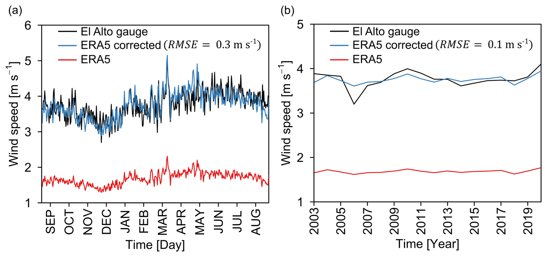
Figure A1Wind speed performance of ERA5-Land evaluated at El Alto gauge in terms of (a) seasonal cycle and (b) interannual variation for the period 2003–2020.
A conceptual lumped model called Air2Water was thus used to estimate LSWT from air temperature (Piccolroaz et al., 2013; Toffolon et al., 2014). The Air2wateR 2.0.0 version available in R was used. ARC-Lake V3 data (MacCallum and Merchant, 2012) available for the period 1995–2012 were used to calibrate and evaluate the Air2wateR model. The spatial resolution of ARC-Lake V3 is 0.05°, and the temporal resolution is daily. The model was calibrated for the period 1995–2003 and evaluated using the period 2004–2012 (see Fig. B1). The performance of Air2Water in the independent control period was acceptable and captured seasonal and interannual variations very well. The LSWT of ARC-Lake V3 had previously been compared with data measured at a buoy located in Lake Titicaca that recorded LSWT (Lazzaro et al., 2021) between 2019 and 2023. The comparison was made between the cell intersecting the measurement point and compared the range of fluctuations and seasonality, since there is no temporal link between the two sources of data. Measured LSWT and LSWT obtained from ARC-Lake V3 fluctuated in a similar range and showed the same seasonal cycle (see Fig. B2).

Figure B1LSWT simulated with the Air2wateR model (Piccolroaz et al., 2013; Toffolon et al., 2014) for Lake Titicaca and its calibration and evaluation performances.
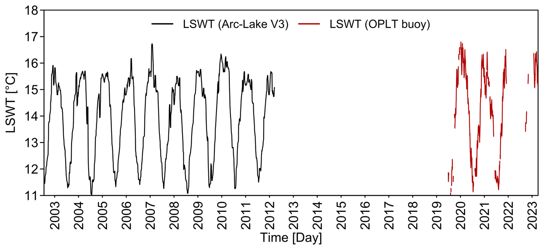
Figure B2LSWT obtained from the buoy site (16.25° S, 68.68° W) in Arc-Lake V3 (MacCallum and Merchant, 2012) and OPLT (Lazzaro et al., 2021).
On-site observations are only available for the Zongo catchment, which is the glacier-dominated catchment adjacent to our study area (see Fig. 1). Streamflows are measured at the Tubo gauge for a catchment of 3.5 km2, of which 52 % is glacierized area. The annual mass balance estimated by the glaciological method (based on direct sampling of changes in the mass of the glacier) was also available for the hydrological period 1991–2016 (see Fig. C1b). The approach used was to obtain the snow and ice model parameters (see the parameters in Fig. 4 and Table C1) in the Zongo catchment and then transfer them directly to BasicModel+IRR+SNOW/ICE. Firstly, the catchment model parameters were calibrated against the streamflow of the Tubo gauge for the hydrological period 2000–2010. The previous 2 hydrological years were used as a warmup period. The irrigation module was disabled because the non-glacierized area was completely dominated by rocks and no crops are cultivated at the high elevations of the Zongo catchment. The parameters with the best performance against the observed streamflow were obtained from 10 000 simulations generated with random hypercube sampling of the Monte Carlo approach. The range of parameters tested is shown in Table C1. NSEsqrt was used as the objective function to select the best-performing parameter sets for the calibration period. Secondly, the model was evaluated against the mass balance observed using the glaciological method (see Sect. 2.5.1) for the period 1992–2016 and using the RMSE criterion. The evaluation was performed with other internal variables of the model, because the goal was to obtain the set of parameters associated with the snow and ice stores. Good internal consistency of the glacier model was thus desirable. In addition, the 25-year time window made it possible to evaluate the ability of the model to simulate the interannual and decadal variation in the mass balance of the Zongo glacier. Figure C1 shows the model's calibration (see Fig. C1a) and evaluation (see Fig. C1b) performances. Figure C1a shows that the model reproduced streamflow reasonably well. Mass balance was also simulated reasonably well. The RMSE obtained (349 mm) is in the range of the error of the mass balance based on the glaciological method (400 mm) (Sicart et al., 2007).
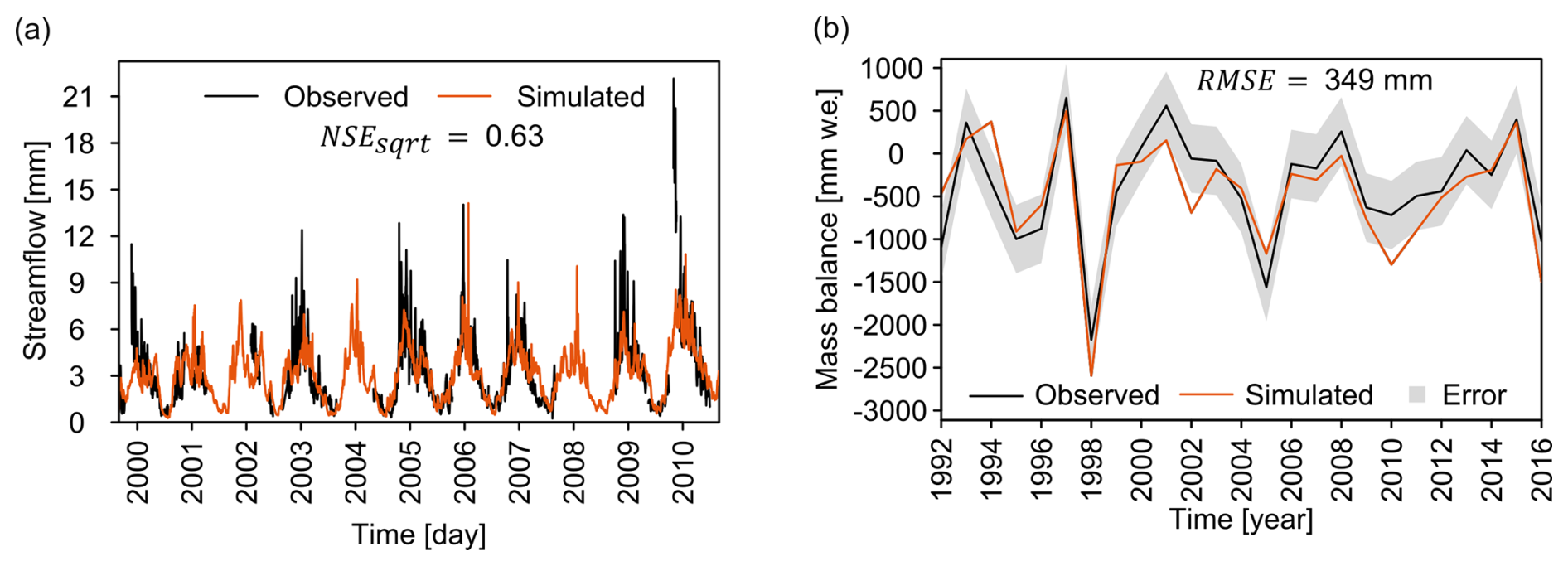
Figure C1Performance of the catchment model in the Zongo catchment versus (a) the observed streamflow at the Tubo gauge and (b) the annual mass balance estimated using the glaciological method. The mass balance estimated using the glaciological method has an error of 400 mm yr−1 (Sicart et al., 2007).
Table C1Parameters of the model implemented in the Zongo catchment and their associated fixed values or ranges tested in order to obtain the parameters of the snow and ice model.
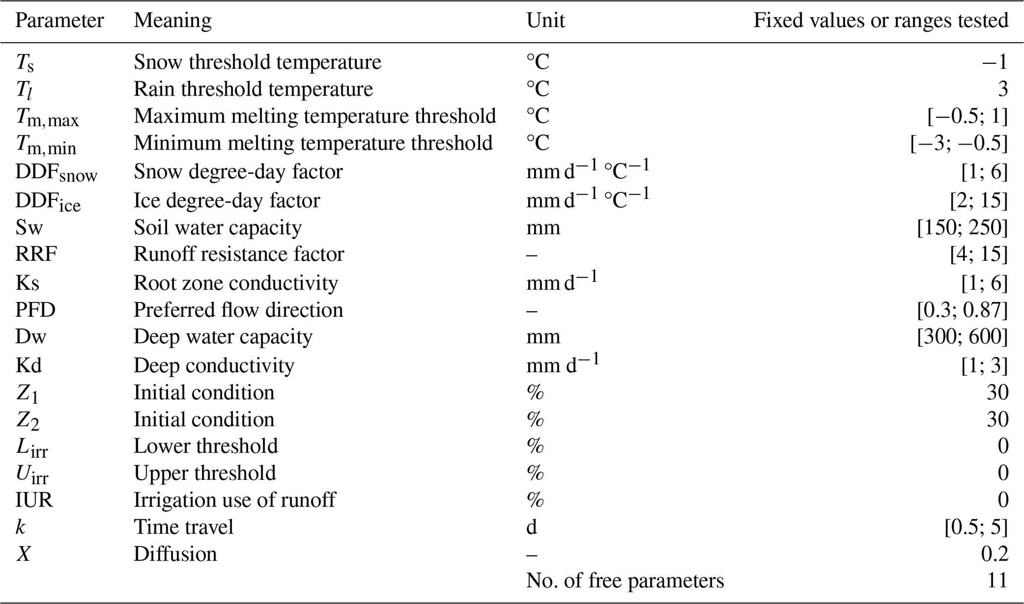

Figure D1Performance of the modeling chain compared with the water levels of Lake Titicaca measured in Puno. Three simulations of water levels are presented because the models produced three different estimates of Qin.
SMM (https://www.weap21.org/webhelp/two-bucket_method.htm, Stockholm Environment Institute, 2025a) and the lake water balance model (https://www.weap21.org/webhelp/river_reservoir_flows.htm, Stockholm Environment Institute, 2025b) are part of WEAP. The models used for the snow processes and lake evaporation are not part of WEAP; therefore, the detailed equations are presented in the Methods section. These models were implemented in WEAP with the user-defined variables (https://www.weap21.org/webhelp/user_defined_variables.htm, Stockholm Environment Institute, 2025c).
The data used in this study are available from their respective websites: GMET (which can be accessed directly from WEAP), ERA5-Land (https://doi.org/10.24381/cds.e2161bac, Muñoz-Sabater, 2019), GLACIOCLIM (https://glacioclim.osug.fr/Glacier-du-Zongo-127, Service d’Observation GLACIOCLIM, 2019), Observatorio Permanente del Lago Titicaca (https://olt.geovisorumsa.com/Datos.html, Institut de Recherche pour le Développement and Instituto de Investigaciones Geográficas, 2020), geodetic mass balance (https://doi.org/10.6096/13, Hugonnet et al., 2021b), and ARC-Lake v3 (https://doi.org/10.17864/1947.186, Merchant and MacCallum, 2018). Measured streamflow and lake water levels should be requested from SENAMHI–Peru and SENAMHI–Bolivia.
NLQ, DR, and TC conceptualized and designed the study approach. AR provided support in the methodological design of the glacier simulation. WLC provided the hydrological and climatic data for the Peruvian side. NLQ and DR implemented the integrated model, analyzed the simulations, and prepared the original version of the manuscript. All the authors contributed to reviewing and editing the manuscript.
The contact author has declared that neither of the authors has any competing interests.
Publisher’s note: Copernicus Publications remains neutral with regard to jurisdictional claims made in the text, published maps, institutional affiliations, or any other geographical representation in this paper. While Copernicus Publications makes every effort to include appropriate place names, the final responsibility lies with the authors.
The authors are grateful to IRD for funding the study. Our special thanks go to SENAMHI–Peru and SENAMHI–Bolivia for providing the ground-based hydroclimatic data. We also thank Javier Núñez (IIGEO-UMSA) and Xavier Lazzaro (IRD) for providing the data from the buoy of the Permanent Observatory of Lake Titicaca. Finally, we thank the other data providers, i.e., GLACIOCLIM (for the Zongo glacier data), THEIA (for access to the geodetic mass balance data), ESA (for access to the ARC-Lake V3 data), ECMWF (for access to the ERA5-Land data), and SEI (for access to the GMET data). The authors are very grateful to Benjamin Kraemer and one anonymous reviewer, who provided a thorough review of this work that helped to improve the final manuscript.
This research has been supported by the Institut de Recherche pour le Développement and Agence Française de Développement (Water Cycle and Climate Change Project – CECC).
This paper was edited by Damien Bouffard and reviewed by Benjamin Kraemer and one anonymous referee.
Allen, R. G., Pereira, L. S., Raes, D., and Smith, M.: Crop evapotranspiration-Guidelines for computing crop water requirements-FAO Irrigation and drainage paper 56, FAO Rome, 300, D05109, ISBN 92-5-104219-5, 1998.
Antonopoulos, V. Z. and Gianniou, S. K.: Simulation of water temperature and dissolved oxygen distribution in Lake Vegoritis, Greece, Ecol. Model., 160, 39–53, https://doi.org/10.1016/S0304-3800(02)00286-7, 2003.
Anyah, R. O., Semazzi, F. H. M., and Xie, L.: Simulated Physical Mechanisms Associated with Climate Variability over Lake Victoria Basin in East Africa, Mon. Weather Rev., 134, 3588–3609, https://doi.org/10.1175/MWR3266.1, 2006.
Ashraf Vaghefi, S., Mousavi, S. J., Abbaspour, K. C., Srinivasan, R., and Arnold, J. R.: Integration of hydrologic and water allocation models in basin-scale water resources management considering crop pattern and climate change: Karkheh River Basin in Iran, Reg. Environ. Change, 15, 475–484, https://doi.org/10.1007/s10113-013-0573-9, 2015.
Autoridad Binacional del Lago Titicaca: Levantamiento hidrográfico convenio binacional del Lago Titicaca, La Paz, Bolivia, https://alt-perubolivia.org/?page_id=1261 (last access: 23 January 2025), 2021.
Autoridad Nacional del Agua: Evaluación de los recursos hídricos en la cuenca del río Ilave, Puno, Perú, https://hdl.handle.net/20.500.12543/3888 (last access: 23 January 2025), 2009.
Autoridad Nacional del Agua: Evaluación de los recursos hídricos en las cuencas de los ríos Huancané y Suches, https://hdl.handle.net/20.500.12543/1736 (last access: 20 April 2023), 2010.
Bai, P. and Wang, Y.: The Importance of Heat Storage for Estimating Lake Evaporation on Different Time Scales: Insights From a Large Shallow Subtropical Lake, Water Resour. Res., 59, e2023WR035123, https://doi.org/10.1029/2023WR035123, 2023.
Barthel, R. and Banzhaf, S.: Groundwater and Surface Water Interaction at the Regional-scale – A Review with Focus on Regional Integrated Models, Water Resour. Manag., 30, 1–32, https://doi.org/10.1007/s11269-015-1163-z, 2016.
Blanken, P. D., Spence, C., Hedstrom, N., and Lenters, J. D.: Evaporation from Lake Superior: 1. Physical controls and processes, J. Gt. Lakes Res., 37, 707–716, https://doi.org/10.1016/j.jglr.2011.08.009, 2011.
Bouchez, C., Goncalves, J., Deschamps, P., Vallet-Coulomb, C., Hamelin, B., Doumnang, J.-C., and Sylvestre, F.: Hydrological, chemical, and isotopic budgets of Lake Chad: a quantitative assessment of evaporation, transpiration and infiltration fluxes, Hydrol. Earth Syst. Sci., 20, 1599–1619, https://doi.org/10.5194/hess-20-1599-2016, 2016.
Buytaert, W., Moulds, S., Acosta, L., Bièvre, B. D., Olmos, C., Villacis, M., Tovar, C., and Verbist, K. M. J.: Glacial melt content of water use in the tropical Andes, Environ. Res. Lett., 12, 114014, https://doi.org/10.1088/1748-9326/aa926c, 2017.
Carenzo, M., Pellicciotti, F., Rimkus, S., and Burlando, P.: Assessing the transferability and robustness of an enhanced temperature-index glacier-melt model, J. Glaciol., 55, 258–274, https://doi.org/10.3189/002214309788608804, 2009.
Carmouze, J.-P.: The energy balance, in: Lake Titicaca, a Synthesis of Limnological Knowledge, Kluwer Academic Publishers, ISBN 0-7923-1663-0, 1992.
Chavoshi, A. and Danesh-Yazdi, M.: Quantifying the uncertainty of lake-groundwater interaction using the forward uncertainty propagation framework: The case of Lake Urmia, J. Hydrol., 610, 127878, https://doi.org/10.1016/j.jhydrol.2022.127878, 2022.
Chebud, Y. A. and Melesse, A. M.: Modelling lake stage and water balance of Lake Tana, Ethiopia, Hydrol. Process., 23, 3534–3544, https://doi.org/10.1002/hyp.7416, 2009.
Clark, M. P. and Slater, A. G.: Probabilistic Quantitative Precipitation Estimation in Complex Terrain, J. Hydrometeorol., 7, 3–22, https://doi.org/10.1175/JHM474.1, 2006.
Delclaux, F., Coudrain, A., and Condom, T.: Evaporation estimation on Lake Titicaca: a synthesis review and modelling, Hydrol. Process., 21, 1664–1677, https://doi.org/10.1002/hyp.6360, 2007.
Duan, Z., Gao, H., and Ke, C.: Estimation of Lake Outflow from the Poorly Gauged Lake Tana (Ethiopia) Using Satellite Remote Sensing Data, Remote Sens., 10, 1060, https://doi.org/10.3390/rs10071060, 2018.
Dussaillant, I., Berthier, E., Brun, F., Masiokas, M., Hugonnet, R., Favier, V., Rabatel, A., Pitte, P., and Ruiz, L.: Two decades of glacier mass loss along the Andes, Nat. Geosci., 12, 802–808, https://doi.org/10.1038/s41561-019-0432-5, 2019.
ESA: Land Cover CCI Product User Guide Version 2.0, https://maps.elie.ucl.ac.be/CCI/viewer/download/ESACCI-LC-Ph2-PUGv2_2.0.pdf (last access: 23 January 2025), 2017.
Fabre, J., Ruelland, D., Dezetter, A., and Grouillet, B.: Simulating past changes in the balance between water demand and availability and assessing their main drivers at the river basin scale, Hydrol. Earth Syst. Sci., 19, 1263–1285, https://doi.org/10.5194/hess-19-1263-2015, 2015.
Farinotti, D., Huss, M., Fürst, J. J., Landmann, J., Machguth, H., Maussion, F., and Pandit, A.: A consensus estimate for the ice thickness distribution of all glaciers on Earth, Nat. Geosci., 12, 168–173, https://doi.org/10.1038/s41561-019-0300-3, 2019.
Frans, C., Istanbulluoglu, E., Lettenmaier, D. P., Naz, B. S., Clarke, G. K. C., Condom, T., Burns, P., and Nolin, A. W.: Predicting glacio-hydrologic change in the headwaters of the Zongo River, Cordillera Real, Bolivia, Water Resour. Res., 51, 9029–9052, https://doi.org/10.1002/2014WR016728, 2015.
Garcia, M., Raes, D., Allen, R., and Herbas, C.: Dynamics of reference evapotranspiration in the Bolivian highlands (Altiplano), Agr. Forest Meteorol., 125, 67–82, https://doi.org/10.1016/j.agrformet.2004.03.005, 2004.
Garcia, M., Raes, D., Jacobsen, S.-E., and Michel, T.: Agroclimatic constraints for rainfed agriculture in the Bolivian Altiplano, J. Arid Environ., 71, 109–121, https://doi.org/10.1016/j.jaridenv.2007.02.005, 2007.
Garreaud, R. and Aceituno, P.: Interannual Rainfall Variability over the South American Altiplano, J. Climate, 14, 2779–2789, https://doi.org/10.1175/1520-0442(2001)014<2779:IRVOTS>2.0.CO;2, 2001.
Garreaud, R., Vuille, M., and Clement, A. C.: The climate of the Altiplano: observed current conditions and mechanisms of past changes, Palaeogeogr. Palaeocl., 194, 5–22, https://doi.org/10.1016/S0031-0182(03)00269-4, 2003.
Geerts, S., Raes, D., Garcia, M., Del Castillo, C., and Buytaert, W.: Agro-climatic suitability mapping for crop production in the Bolivian Altiplano: A case study for quinoa, Agr. Forest Meteorol., 139, 399–412, https://doi.org/10.1016/j.agrformet.2006.08.018, 2006.
Githui, F., Thayalakumaran, T., and Selle, B.: Estimating irrigation inputs for distributed hydrological modelling: a case study from an irrigated catchment in southeast Australia, Hydrol. Process., 30, 1824–1835, https://doi.org/10.1002/hyp.10757, 2016.
Gronewold, A. D., Bruxer, J., Durnford, D., Smith, J. P., Clites, A. H., Seglenieks, F., Qian, S. S., Hunter, T. S., and Fortin, V.: Hydrological drivers of record-setting water level rise on Earth's largest lake system, Water Resour. Res., 52, 4026–4042, https://doi.org/10.1002/2015WR018209, 2016.
Gronewold, A. D., Fortin, V., Caldwell, R., and Noel, J.: Resolving Hydrometeorological Data Discontinuities along an International Border, B. Am. Meteorol. Soc., 99, 899–910, https://doi.org/10.1175/BAMS-D-16-0060.1, 2018.
Gu, H., Ma, Z., and Li, M.: Effect of a large and very shallow lake on local summer precipitation over the Lake Taihu basin in China, J. Geophys. Res.-Atmos., 121, 8832–8848, https://doi.org/10.1002/2015JD024098, 2016.
Guo, Y., Zhang, Y., Zhang, L., and Wang, Z.: Regionalization of hydrological modeling for predicting streamflow in ungauged catchments: A comprehensive review, WIREs Water, 8, e1487, https://doi.org/10.1002/wat2.1487, 2021.
Hall, D. K., Riggs, G. A., Salomonson, V. V., DiGirolamo, N. E., and Bayr, K. J.: MODIS snow-cover products, Remote Sens. Environ., 83, 181–194, https://doi.org/10.1016/S0034-4257(02)00095-0, 2002.
Hassanzadeh, E., Zarghami, M., and Hassanzadeh, Y.: Determining the Main Factors in Declining the Urmia Lake Level by Using System Dynamics Modeling, Water Resour. Manag., 26, 129–145, https://doi.org/10.1007/s11269-011-9909-8, 2012.
Herrera, S. L., Meneses, R. I., and Anthelme, F.: Comunidades vegetales de los bofedales de la Cordillera Real (Bolivia) bajo el calentamiento global, Ecol. En Boliv., 50, 39–56, 2015.
Hock, R.: Temperature index melt modelling in mountain areas, J. Hydrol., 282, 104–115, https://doi.org/10.1016/S0022-1694(03)00257-9, 2003.
Hong, Y., Xuan Do, H., Kessler, J., Fry, L., Read, L., Rafieei Nasab, A., Gronewold, A. D., Mason, L., and Anderson, E. J.: Evaluation of gridded precipitation datasets over international basins and large lakes, J. Hydrol., 607, 127507, https://doi.org/10.1016/j.jhydrol.2022.127507, 2022.
Hosseini-Moghari, S.-M., Araghinejad, S., Tourian, M. J., Ebrahimi, K., and Döll, P.: Quantifying the impacts of human water use and climate variations on recent drying of Lake Urmia basin: the value of different sets of spaceborne and in situ data for calibrating a global hydrological model, Hydrol. Earth Syst. Sci., 24, 1939–1956, https://doi.org/10.5194/hess-24-1939-2020, 2020.
Hublart, P., Ruelland, D., García de Cortázar-Atauri, I., Gascoin, S., Lhermitte, S., and Ibacache, A.: Reliability of lumped hydrological modeling in a semi-arid mountainous catchment facing water-use changes, Hydrol. Earth Syst. Sci., 20, 3691–3717, https://doi.org/10.5194/hess-20-3691-2016, 2016.
Hugonnet, R., McNabb, R., Berthier, E., Menounos, B., Nuth, C., Girod, L., Farinotti, D., Huss, M., Dussaillant, I., Brun, F., and Kääb, A.: Accelerated global glacier mass loss in the early twenty-first century, Nature, 592, 726–731, https://doi.org/10.1038/s41586-021-03436-z, 2021a.
Hugonnet, R., McNabb, R., and Berthier, E.: Accelerated global glacier mass loss in the early twenty-first century – Dataset, SEDOO [data set], https://doi.org/10.6096/13, 2021b.
Instituto Nacional de Recursos Naturales: Actualización del Balance Hídrico de la Cuenca del río Ramis, Ayaviri, Perú, https://hdl.handle.net/20.500.12543/3294 (last access: 23 January 2025), 2008.
Instituto Nacional de Estadística: Censo agropecuario Estado Plurinacional de Bolivia, 2013, https://anda.ine.gob.bo/index.php/catalog/24 (last access: 19 April 2023), 2015.
Institut de Recherche pour le Développement and Instituto de Investigaciones Geográficas: Observatorio permanente del Lago Titicaca, GEOVISORUMSA, https://olt.geovisorumsa.com/Datos.html (last access: 23 January 2025), 2020.
INTECSA, AIC, and CNR: Plan Director Global Binacional de Protección – Prevención de Inundaciones y Aprovechamiento de los Recursos del Lago Titicaca, Rio Desaguadero, Lago Poopó y Lago Salar Coipasa (Sistema T.D.P.S.): Estudio de hidrogeología, https://observatorio.alt-perubolivia.org/storage/multi/F2O7VRdzZQ3CsBWscLA5vmgBd6NnyDfOGmyxQcuF.pdf (last access: 23 January 2025), 1993a.
INTECSA, AIC, and CNR: Plan Director Global Binacional de Protección – Prevención de Inundaciones y Aprovechamiento de los Recursos del Lago Titicaca, Rio Desaguadero, Lago Poopó y Lago Salar Coipasa (Sistema T.D.P.S.): Modelo Matemáticos del Sistema Hídrico T.D.P.S., https://observatorio.alt-perubolivia.org/storage/multi/4K2jIZWhcmR4lYd9NnIN7RMFetkHH7bELwe4i5Bi.pdf (last access: 23 January 2025), 1993b.
INTECSA, AIC, and CNR: Plan Director Global Binacional de Protección – Prevención de Inundaciones y Aprovechamiento de los Recursos del Lago Titicaca, Rio Desaguadero, Lago Poopó y Lago Salar de Coipasa (Sistema T.D.P.S.): Diagnostico Socioeconómico, https://observatorio.alt-perubolivia.org/storage/multi/2TSepRCV8jXuAYFJSTIMU6wMU7jXBIyKRNaeYV6T.pdf (last access: 23 January 2025), 1993c.
Jarvis, A., Reuter, H. I., Nelson, A., and Guevara, E.: Hole-filled SRTM for the globe Version 4, available from the CGIAR-CSI SRTM 90m Database, https://srtm.csi.cgiar.org (last access: 23 January 2025), 2008.
Jonaitis, J. A., Perry, L. B., Soulé, P. T., Thaxton, C., Andrade-Flores, M. F., Vargas, T. I., and Ticona, L.: Spatiotemporal patterns of ENSO-precipitation relationships in the tropical Andes of southern Peru and Bolivia, Int. J. Climatol., 41, 4061–4076, https://doi.org/10.1002/joc.7058, 2021.
Kannan, N., Jeong, J., and Srinivasan, R.: Hydrologic Modeling of a Canal-Irrigated Agricultural Watershed with Irrigation Best Management Practices: Case Study, J. Hydrol. Eng., 16, 746–757, https://doi.org/10.1061/(ASCE)HE.1943-5584.0000364, 2011.
Kebede, S., Travi, Y., Alemayehu, T., and Marc, V.: Water balance of Lake Tana and its sensitivity to fluctuations in rainfall, Blue Nile basin, Ethiopia, J. Hydrol., 316, 233–247, https://doi.org/10.1016/j.jhydrol.2005.05.011, 2006.
Kizza, M., Westerberg, I., Rodhe, A., and Ntale, H. K.: Estimating areal rainfall over Lake Victoria and its basin using ground-based and satellite data, J. Hydrol., 464–465, 401–411, https://doi.org/10.1016/j.jhydrol.2012.07.024, 2012.
Lazzaro, X., Achá Cordero, D., Cruz Hernández, V., Duarte Tejerina, J., Justiniano Ayllón, M., Lanza Aguilar, G., Maldonado Alfaro, J., Molina Arzabe, C., Nuñez Villalba, J., Ormachea Rojas, M., and Sterling, P.: HydroMet: La primera boya automática perfiladora con alta-frecuencia en el Lago Titicaca, el más alto de los Grandes Lagos del mundo, Ecol. En Boliv., 56, 65–67, 2021.
Lenters, J. D., Kratz, T. K., and Bowser, C. J.: Effects of climate variability on lake evaporation: Results from a long-term energy budget study of Sparkling Lake, northern Wisconsin (USA), J. Hydrol., 308, 168–195, https://doi.org/10.1016/j.jhydrol.2004.10.028, 2005.
Lima-Quispe, N., Escobar, M., Wickel, A. J., von Kaenel, M., and Purkey, D.: Untangling the effects of climate variability and irrigation management on water levels in Lakes Titicaca and Poopó, J. Hydrol. Reg. Stud., 37, 100927, https://doi.org/10.1016/j.ejrh.2021.100927, 2021.
MacCallum, S. N. and Merchant, C. J.: Surface water temperature observations of large lakes by optimal estimation, Can. J. Remote Sens., 38, 25–45, https://doi.org/10.5589/m12-010, 2012.
Maidment, D. R.: Handbook of hydrology, McGraw-Hill, New York, ISBN 9780071711777, 1993.
McInerney, D., Thyer, M., Kavetski, D., Githui, F., Thayalakumaran, T., Liu, M., and Kuczera, G.: The Importance of Spatiotemporal Variability in Irrigation Inputs for Hydrological Modeling of Irrigated Catchments, Water Resour. Res., 54, 6792–6821, https://doi.org/10.1029/2017WR022049, 2018.
Merchant, C. and MacCallum, S.: Lake Surface Water Temperature ARC-Lake v3 (1995–2012), University of Reading [data set], https://doi.org/10.17864/1947.186, 2018.
Millan, R., Mouginot, J., Rabatel, A., and Morlighem, M.: Ice velocity and thickness of the world's glaciers, Nat. Geosci., 15, 124–129, https://doi.org/10.1038/s41561-021-00885-z, 2022.
Ministerio de Desarrollo Rural y Tierras: Mapa de Cobertura y Uso Actual de la Tierra de Bolivia 2010, La Paz, Bolivia, https://cdrnbolivia.com/cdrnb/geografia-fisica-nacional/cobertura_uso_2010.zip (last access: 23 November 2022), 2011.
Ministerio de Medio Ambiente y Agua: Inventario Nacional de Sistemas de Riego 2012, https://www.bivica.org/files/sistemas-riego-inventario.pdf (last access: 23 January 2025), 2013.
Ministerio de Medio Ambiente y Agua: Balance hídrico superficial de Bolivia (1980–2016), https://datos.siarh.gob.bo/biblioteca/406 (last access: 10 February 2024), 2018.
Ministerio del Ambiente: Mapa Nacional de Cobertura Vegetal, Lima, Perú, https://www.minam.gob.pe/patrimonio-natural/wp-content/uploads/sites/6/2013/10/MAPA-NACIONAL-DE-COBERTURA-VEGETAL-FINAL.compressed.pdf (last access: 23 January 2025), 2015.
Muñoz-Sabater, J.: ERA5-Land hourly data from 1950 to present, Copernicus Climate Change Service (C3S) Climate Data Store (CDS) [data set], https://doi.org/10.24381/cds.e2161bac, 2019.
Muñoz-Sabater, J., Dutra, E., Agustí-Panareda, A., Albergel, C., Arduini, G., Balsamo, G., Boussetta, S., Choulga, M., Harrigan, S., Hersbach, H., Martens, B., Miralles, D. G., Piles, M., Rodríguez-Fernández, N. J., Zsoter, E., Buontempo, C., and Thépaut, J.-N.: ERA5-Land: a state-of-the-art global reanalysis dataset for land applications, Earth Syst. Sci. Data, 13, 4349–4383, https://doi.org/10.5194/essd-13-4349-2021, 2021.
Nash, J. E. and Sutcliffe, J. V.: River flow forecasting through conceptual models part I – A discussion of principles, J. Hydrol., 10, 282–290, https://doi.org/10.1016/0022-1694(70)90255-6, 1970.
Newman, A. J., Clark, M. P., Craig, J., Nijssen, B., Wood, A., Gutmann, E., Mizukami, N., Brekke, L., and Arnold, J. R.: Gridded ensemble precipitation and temperature estimates for the contiguous United States, J. Hydrometeorol., 16, 2481–2500, 2015.
Nicholson, S. E.: Lake-effect rainfall over Africa's great lakes and other lakes in the rift valleys, J. Gt. Lakes Res., 49, 101971, https://doi.org/10.1016/j.jglr.2021.12.004, 2023.
Niswonger, R. G., Allander, K. K., and Jeton, A. E.: Collaborative modelling and integrated decision support system analysis of a developed terminal lake basin, J. Hydrol., 517, 521–537, https://doi.org/10.1016/j.jhydrol.2014.05.043, 2014.
Oudin, L., Andréassian, V., Mathevet, T., Perrin, C., and Michel, C.: Dynamic averaging of rainfall-runoff model simulations from complementary model parameterizations, Water Resour. Res., 42, W07410, https://doi.org/10.1029/2005WR004636, 2006.
Parizi, E., Hosseini, S. M., Ataie-Ashtiani, B., and Nikraftar, Z.: Quantifying lake–aquifer water exchange: the case of Lake Urmia, Iran, Hydrol. Sci. J., 67, 725–740, https://doi.org/10.1080/02626667.2022.2044044, 2022.
Penman, H. L.: Natural evaporation from open water, bare soil and grass, P. R. Soc. Lond. A Math., 193, 120–145, 1948.
Piccolroaz, S., Toffolon, M., and Majone, B.: A simple lumped model to convert air temperature into surface water temperature in lakes, Hydrol. Earth Syst. Sci., 17, 3323–3338, https://doi.org/10.5194/hess-17-3323-2013, 2013.
Pillco Zolá, R., Bengtsson, L., Berndtsson, R., Martí-Cardona, B., Satgé, F., Timouk, F., Bonnet, M.-P., Mollericon, L., Gamarra, C., and Pasapera, J.: Modelling Lake Titicaca's daily and monthly evaporation, Hydrol. Earth Syst. Sci., 23, 657–668, https://doi.org/10.5194/hess-23-657-2019, 2019.
Pôças, I., Calera, A., Campos, I., and Cunha, M.: Remote sensing for estimating and mapping single and basal crop coefficientes: A review on spectral vegetation indices approaches, Agr. Water Manage., 233, 106081, https://doi.org/10.1016/j.agwat.2020.106081, 2020.
Rabatel, A., Francou, B., Soruco, A., Gomez, J., Cáceres, B., Ceballos, J. L., Basantes, R., Vuille, M., Sicart, J.-E., Huggel, C., Scheel, M., Lejeune, Y., Arnaud, Y., Collet, M., Condom, T., Consoli, G., Favier, V., Jomelli, V., Galarraga, R., Ginot, P., Maisincho, L., Mendoza, J., Ménégoz, M., Ramirez, E., Ribstein, P., Suarez, W., Villacis, M., and Wagnon, P.: Current state of glaciers in the tropical Andes: a multi-century perspective on glacier evolution and climate change, The Cryosphere, 7, 81–102, https://doi.org/10.5194/tc-7-81-2013, 2013.
Revollo, M. M.: Management issues in the Lake Titicaca and Lake Poopo system: Importance of developing a water budget, Lakes Reserv. Sci. Policy Manag. Sustain. Use, 6, 225–229, https://doi.org/10.1046/j.1440-1770.2001.00151.x, 2001.
RGI Consortium: Randolph Glacier Inventory – A Dataset of Global Glacier Outlines, Version 6, National Snow and Ice Data Center [data set], https://doi.org/10.7265/4m1f-gd79, 2017.
Rieckermann, J., Daebel, H., Ronteltap, M., and Bernauer, T.: Assessing the performance of international water management at Lake Titicaca, Aquat. Sci., 68, 502–516, https://doi.org/10.1007/s00027-006-0863-0, 2006.
Rientjes, T. H. M., Perera, B. U. J., Haile, A. T., Reggiani, P., and Muthuwatta, L. P.: Regionalisation for lake level simulation – the case of Lake Tana in the Upper Blue Nile, Ethiopia, Hydrol. Earth Syst. Sci., 15, 1167–1183, https://doi.org/10.5194/hess-15-1167-2011, 2011.
Roche, M. A., Bourges, J., Cortes, J., and Mattos, R.: Climatology And Hydrology, in: Lake Titicaca: A Synthesis of Limnological Knowledge, edited by: Dejoux, C. and Iltis, A., Springer Netherlands, Dordrecht, 63–88, https://doi.org/10.1007/978-94-011-2406-5_4, 1992.
Ruelland, D.: Should altitudinal gradients of temperature and precipitation inputs be inferred from key parameters in snow-hydrological models?, Hydrol. Earth Syst. Sci., 24, 2609–2632, https://doi.org/10.5194/hess-24-2609-2020, 2020.
Ruelland, D.: Development of the snow- and ice-accounting routine (SIAR), J. Hydrol., 624, 129867, https://doi.org/10.1016/j.jhydrol.2023.129867, 2023.
Satgé, F., Ruelland, D., Bonnet, M.-P., Molina, J., and Pillco, R.: Consistency of satellite-based precipitation products in space and over time compared with gauge observations and snow- hydrological modelling in the Lake Titicaca region, Hydrol. Earth Syst. Sci., 23, 595–619, https://doi.org/10.5194/hess-23-595-2019, 2019.
Schulz, S., Darehshouri, S., Hassanzadeh, E., Tajrishy, M., and Schüth, C.: Climate change or irrigated agriculture – what drives the water level decline of Lake Urmia, Sci. Rep., 10, 236, https://doi.org/10.1038/s41598-019-57150-y, 2020.
Scott, R. W. and Huff, F. A.: Impacts of the Great Lakes on Regional Climate Conditions, J. Gt. Lakes Res., 22, 845–863, https://doi.org/10.1016/S0380-1330(96)71006-7, 1996.
Segura, H., Espinoza, J. C., Junquas, C., and Takahashi, K.: Evidencing decadal and interdecadal hydroclimatic variability over the Central Andes, Environ. Res. Lett., 11, 094016, https://doi.org/10.1088/1748-9326/11/9/094016, 2016.
Seibert, J., Vis, M. J. P., Kohn, I., Weiler, M., and Stahl, K.: Technical note: Representing glacier geometry changes in a semi-distributed hydrological model, Hydrol. Earth Syst. Sci., 22, 2211–2224, https://doi.org/10.5194/hess-22-2211-2018, 2018.
Sene, K. J. and Plinston, D. T.: A review and update of the hydrology of Lake Victoria in East Africa, Hydrolog. Sci. J., 39, 47–63, https://doi.org/10.1080/02626669409492719, 1994.
Service d'Observation GLACIOCLIM: Zongo glacier, GLACIOCLIM [data set], https://glacioclim.osug.fr/Glacier-du-Zongo-127 (last access: 23 January 2025), 2019.
Shadkam, S., Ludwig, F., van Oel, P., Kirmit, Ç., and Kabat, P.: Impacts of climate change and water resources development on the declining inflow into Iran's Urmia Lake, J. Gt. Lakes Res., 42, 942–952, https://doi.org/10.1016/j.jglr.2016.07.033, 2016.
Shea, J. M., Moore, R. D., and Stahl, K.: Derivation of melt factors from glacier mass-balance records in western Canada, J. Glaciol., 55, 123–130, https://doi.org/10.3189/002214309788608886, 2009.
Sicart, J. E., Ribstein, P., Francou, B., Pouyaud, B., and Condom, T.: Glacier mass balance of tropical Zongo glacier, Bolivia, comparing hydrological and glaciological methods, Global Planet. Change, 59, 27–36, https://doi.org/10.1016/j.gloplacha.2006.11.024, 2007.
Sicart, J. E., Hock, R., and Six, D.: Glacier melt, air temperature, and energy balance in different climates: The Bolivian Tropics, the French Alps, and northern Sweden, J. Geophys. Res.-Atmos., 113, D24113, https://doi.org/10.1029/2008JD010406, 2008.
Sicart, J. E., Hock, R., Ribstein, P., and Chazarin, J. P.: Sky longwave radiation on tropical Andean glaciers: parameterization and sensitivity to atmospheric variables, J. Glaciol., 56, 854–860, https://doi.org/10.3189/002214310794457182, 2010.
Soruco, A., Vincent, C., Rabatel, A., Francou, B., Thibert, E., Sicart, J. E., and Condom, T.: Contribution of glacier runoff to water resources of La Paz city, Bolivia (16° S), Ann. Glaciol., 56, 147–154, https://doi.org/10.3189/2015AoG70A001, 2015.
Sterner, R. W., Keeler, B., Polasky, S., Poudel, R., Rhude, K., and Rogers, M.: Ecosystem services of Earth's largest freshwater lakes, Ecosyst. Serv., 41, 101046, https://doi.org/10.1016/j.ecoser.2019.101046, 2020.
Stockholm Environment Institute: WEAP21-Soil Moisture Method, https://www.weap21.org/webhelp/two-bucket_method.htm (last access: 29 January 2025), 2025a.
Stockholm Environment Institute: WEAP21-River Reservoir Flows, https://www.weap21.org/webhelp/river_reservoir_flows.htm, last access (29 January 2025), 2025b.
Stockholm Environment Institute: WEAP21-Customizing Data Variables, https://www.weap21.org/webhelp/user_defined_variables.htm (last access: 29 January 2025), 2025c.
Su, D., Wen, L., Gao, X., Leppäranta, M., Song, X., Shi, Q., and Kirillin, G.: Effects of the Largest Lake of the Tibetan Plateau on the Regional Climate, J. Geophys. Res.-Atmos., 125, e2020JD033396, https://doi.org/10.1029/2020JD033396, 2020.
Sulca, J., Apaéstegui, J., and Tacza, J.: New insights into the biennial-to-multidecadal variability of the water level fluctuation in Lake Titicaca in the 20th century, Front. Clim., 5, 1325224, https://doi.org/10.3389/fclim.2023.1325224, 2024.
Thiery, W., Davin, E. L., Panitz, H.-J., Demuzere, M., Lhermitte, S., and van Lipzig, N.: The Impact of the African Great Lakes on the Regional Climate, J. Climate, 28, 4061–4085, https://doi.org/10.1175/JCLI-D-14-00565.1, 2015.
Toffolon, M., Piccolroaz, S., Majone, B., Soja, A.-M., Peeters, F., Schmid, M., and Wüest, A.: Prediction of surface temperature in lakes with different morphology using air temperature, Limnol. Oceanogr., 59, 2185–2202, https://doi.org/10.4319/lo.2014.59.6.2185, 2014.
Vanderkelen, I., van Lipzig, N. P. M., and Thiery, W.: Modelling the water balance of Lake Victoria (East Africa) – Part 1: Observational analysis, Hydrol. Earth Syst. Sci., 22, 5509–5525, https://doi.org/10.5194/hess-22-5509-2018, 2018.
Vaquero, G., Siavashani, N. S., García-Martínez, D., Elorza, F. J., Bila, M., Candela, L., and Serrat-Capdevila, A.: The Lake Chad transboundary aquifer. Estimation of groundwater fluxes through international borders from regional numerical modeling, J. Hydrol. Reg. Stud., 38, 100935, https://doi.org/10.1016/j.ejrh.2021.100935, 2021.
Wale, A., Rientjes, T. H. M., Gieske, A. S. M., and Getachew, H. A.: Ungauged catchment contributions to Lake Tana's water balance, Hydrol. Process., 23, 3682–3693, https://doi.org/10.1002/hyp.7284, 2009.
Wang, W., Lee, X., Xiao, W., Liu, S., Schultz, N., Wang, Y., Zhang, M., and Zhao, L.: Global lake evaporation accelerated by changes in surface energy allocation in a warmer climate, Nat. Geosci., 11, 410–414, https://doi.org/10.1038/s41561-018-0114-8, 2018.
Winter, J. M., Young, C. A., Mehta, V. K., Ruane, A. C., Azarderakhsh, M., Davitt, A., McDonald, K., Haden, V. R., and Rosenzweig, C.: Integrating water supply constraints into irrigated agricultural simulations of California, Environ. Modell. Softw., 96, 335–346, https://doi.org/10.1016/j.envsoft.2017.06.048, 2017.
Wu, B., Tian, F., Zhang, M., Piao, S., Zeng, H., Zhu, W., Liu, J., Elnashar, A., and Lu, Y.: Quantifying global agricultural water appropriation with data derived from earth observations, J. Clean. Prod., 358, 131891, https://doi.org/10.1016/j.jclepro.2022.131891, 2022.
Wurtsbaugh, W. A., Miller, C., Null, S. E., DeRose, R. J., Wilcock, P., Hahnenberger, M., Howe, F., and Moore, J.: Decline of the world's saline lakes, Nat. Geosci., 10, 816–821, https://doi.org/10.1038/ngeo3052, 2017.
Xu, S., Frey, S. K., Erler, A. R., Khader, O., Berg, S. J., Hwang, H. T., Callaghan, M. V., Davison, J. H., and Sudicky, E. A.: Investigating groundwater-lake interactions in the Laurentian Great Lakes with a fully-integrated surface water-groundwater model, J. Hydrol., 594, 125911, https://doi.org/10.1016/j.jhydrol.2020.125911, 2021.
Yao, F., Livneh, B., Rajagopalan, B., Wang, J., Crétaux, J.-F., Wada, Y., and Berge-Nguyen, M.: Satellites reveal widespread decline in global lake water storage, Science, 380, 743–749, https://doi.org/10.1126/science.abo2812, 2023.
Yates, D., Sieber, J., Purkey, D., and Huber-Lee, A.: WEAP21 – A demand-, priority-, and preference-driven water planning model: part 1: model characteristics, Water Int., 30, 487–500, 2005.
Zhang, Y. and Post, D.: How good are hydrological models for gap-filling streamflow data?, Hydrol. Earth Syst. Sci., 22, 4593–4604, https://doi.org/10.5194/hess-22-4593-2018, 2018.
- Abstract
- Introduction
- Material
- Method
- Results
- Discussion and conclusions
- Appendix A: Performance of the ERA5-Land dataset
- Appendix B: Simulation of LSWT
- Appendix C: Parameters of the snow and ice model
- Appendix D: Simulated and observed water levels
- Code availability
- Data availability
- Author contributions
- Competing interests
- Disclaimer
- Acknowledgements
- Financial support
- Review statement
- References