Assessing the cumulative impact of on-farm reservoirs on modeled surface hydrology

On-farm reservoirs (OFRs) are crucial water bodies for meeting global irrigation needs. Farmers use OFRs to store water from precipitation and runoff during the rainy season, which they then use to irrigate their crops during the dry season. Despite their importance to crop irrigation, OFRs can have a cumulative impact on surface hydrology by decreasing flow and peak flow. Nonetheless, there is limited knowledge on the spatial and temporal variability of the OFRs' impacts. Therefore, to gain an understanding of the cumulative impact of OFRs on surface hydrology, we propose a novel framework that integrates a top-down, data-driven, remote sensing-based algorithm with physically based models, leveraging the latest developments in the Soil Water Assessment Tool+ (SWAT+). We assessed the impact of OFRs in a watershed located in eastern Arkansas, the third most irrigated state in the USA. Our results indicate that the presence of OFRs in the watershed is associated with a decrease in annual flow of 14 %–24 % and a mean reduction in peak flow of 43 %–60 %. In addition, the cumulative impact of the OFRs was not equally distributed across the watershed, varying according to the OFR spatial distribution and their storage capacity. The results of this study and the proposed framework can support water agencies with information on the cumulative impact of OFRs, aiming to support surface water resources management. This is relevant because the number of OFRs is expected to increase globally as a response to climate change under severe drought conditions.

1 Introduction

Inland water bodies (e.g., lakes and reservoirs) comprise a small fraction of Earth's surface; however, they are responsible for storing the vast majority of the accessible freshwater resources available on Earth. In addition, these water bodies are pivotal components of surface hydrology, playing key roles in ecosystem functioning and providing habitats for wildlife (Khazaei et al., 2022; Verpoorter et al., 2014). In particular, on-farm reservoirs (OFRs) are crucial for meeting global irrigation needs (Döll et al., 2009; Downing, 2010; Van Den Hoek et al., 2019). Farmers use OFRs to store water from precipitation and runoff during the rainy season to irrigate their crops during the dry season (Habets et al., 2018; Perin et al., 2021b; Vanthof and Kelly, 2019; Yaeger et al., 2017, 2018). The number of OFRs is expected to rise worldwide in the coming decades, and estimates show that there are more than 2.1 million OFRs in the US alone (Downing, 2010; Renwick et al., 2005). OFRs are often built to manage surface water resources more efficiently and to help mitigate the impact of extreme droughts, which are projected to increase due to climate change (Habets et al., 2018; Van Der Zaag and Gupta, 2008). Although OFRs are small water bodies (<50 ha), they can have cumulative impacts on the local and remote hydrology in the watersheds where they occur (e.g., decreasing flow and peak flow) (Habets et al., 2018). Their impact may contribute to worsening the surface water stress already intensified by climate change and population growth (Vörösmarty et al., 2010). Most studies have focused on the cumulative impact of major large reservoirs on downstream flow alteration (Chalise et al., 2021; Mukhopadhyay et al., 2021), but limited analysis has been performed on the impact of OFRs on downstream flow availability.

To quantify the impact of OFRs on surface hydrology, it is necessary to understand the spatial and temporal variability of surface water extent in OFRs, as well as how the impacts are related to the OFR networks, as the impacts of OFRs are not the sum of the individual OFR impacts, but rather the sum and their interaction effects (Canter and Kamath, 1995; Habets et al., 2018). By gathering information from several studies conducted in different countries (e.g., the USA, France, Brazil), Habets et al. (2018) conducted a thorough assessment of the OFRs' impact on surface hydrology and the various types of models and methods for representing OFRs within the watershed. The authors concluded that the modeled OFR impacts have a wide range, and that most studies reported a mean annual reduction in flow, which ranged from 0.2 % to 36 %. In addition, the variability of the impact, as identified in these previous studies, was higher when assessing low flows over multiple years, with reductions ranging from 0.3 % to 60 %. In general, the estimated mean annual reduction in flow was 13.4±8.0 %, and the mean decrease in peak flow was up to 45 % (Habets et al., 2018).

The approaches used to quantify the cumulative impact of OFRs can be divided into two classes: data-driven methods and process-based hydrological modeling. The data-driven approaches include three primary methods. The first method relies on assessing measured inflows and outflows of selected OFRs, aiming to quantify their hydrological functioning with the assumption that the cumulative impacts are the sum of individual impacts (Culler et al., 1961; Dubreuil and Girard, 1973; Kennon, 1966). A variation of the cumulative impact assessment approach has been recently suggested by Hwang et al. (2021) for comparing naturalized flows and controlled flows to assess the impact of large reservoir systems. The second method is based on statistical analysis of the observed discharge time series of a watershed as the number of OFRs increased (Galéa et al., 2005; Schreider et al., 2002). This approach is limited when discriminating the specific impact of OFRs from those of land use and land cover change, and when explicitly representing the OFRs in the models, given that OFRs tend to be aggregated within the entire basin (i.e., OFRs surface area and/or storage are summed and modeled as a unique water impoundment). The third method involves conducting a paired-catchment experiment by comparing the flows from two adjacent and similar catchments: one with OFRs and the other without OFRs (Thompson, 2012). This technique requires the catchment properties (e.g., soils, topology, lithology, land cover) to be spatially homogeneous, which is practically nonexistent at a large scale, hence, this method's applications are limited.

The second class of methods relates to hydrological modeling, which is the most widely used approach for assessing the impacts of OFRs. A variety of models have been proposed by coupling the OFRs' water balance with a quantitative approach to estimate the OFRs' water volume change (Fowler et al., 2015; Habets et al., 2014; Jalowska and Yuan, 2019; Yongbo et al., 2014; Ni and Parajuli, 2018; Perrin et al., 2012; Zhang et al., 2012). In general, the models have three main components: the OFR water balance, a quantitative approach to quantify OFR inflows, and a spatial representation of the OFR's network. These different model components result in various limitations and assumptions – a comprehensive assessment of these three components and their impact on hydrological simulations is provided in a recent review (Habets et al., 2018). Therefore, when selecting a specific model to assess the impacts of the OFRs, it is essential to consider the model's suitability for addressing the target issue, as well as its limitations and assumptions. The selected model should also have the capability to incorporate and assimilate varying land-surface conditions (e.g., soil moisture) and time-varying OFR storages, which can be obtained either from local monitoring or through remote sensing.

Most studies have used remotely-sensed products such as soil moisture (e.g., SMAP; Entekhabi et al., 2010), groundwater (e.g., GRACE; Tapley et al., 2004) and land cover conditions (e.g., MODIS; Justice et al., 1998) for assimilating current conditions into hydrological models. Given that OFRs tend to occur in high numbers (e.g., hundreds), multiple studies leveraged the latest developments and availability of satellite imagery to monitor the occurrence and dynamics of OFRs (Jones et al., 2017; Ogilvie et al., 2018, 2020; Perin et al., 2022, 2021a, b; Van Den Hoek et al., 2019; Vanthof and Kelly, 2019), which could provide helpful information on local storage conditions for predicting downstream streamflow. Furthermore, these studies enabled the quantification of the number of OFRs and their spatial and temporal variability in surface water areas and storage within the watershed where they occur, providing relevant information for modeling the cumulative impact of OFRs. Despite the complementary information provided by satellite imagery, there are only a few studies that incorporated remote sensing-derived information (e.g., soil moisture derived from SMAP, groundwater based on GRACE) with hydrological modeling (Ni and Parajuli, 2018; Yongbo et al., 2014; Zhang et al., 2012), and these studies are limited to mapping the OFRs occurrence, or to snapshots of the OFRs conditions (e.g., surface area). To the best of our knowledge, no study has combined the spatial and temporal variability of the OFRs – derived from multi-year satellite imagery time series analyses – with a process-based hydrological model.

Therefore, to gain an understanding of the cumulative impact of OFRs on surface hydrology, this study proposes a new approach that systematically integrates the dynamically varying conditions of OFRs based on satellite imagery time series (Perin et al., 2022) using a top-down data-driven approach within the latest SWAT+ model. The Soil and Water Assessment Tool (SWAT) (Arnold et al., 2012) has been widely used to model the impacts of the OFRs (Jalowska and Yuan, 2019; Kim and Parajuli, 2014; Ni et al., 2020; Ni and Parajuli, 2018; Perrin et al., 2012; Rabelo et al., 2021; Yongbo et al., 2014; Zhang et al., 2012), in part given by a comprehensive collection of model documentation and guidelines available online (https://swat.tamu.edu/, last access: 11 January 2022). Our objectives are to (1) assess the spatial and temporal variability of the cumulative impact of OFRs at the watershed and subwatershed levels, and (2) to quantify the intra- and interannual impacts of the OFRs on flow and peak flow at the channel scale. By integrating the SWAT+ model with a remote sensing assimilation algorithm to account for the OFRs spatial variability – which is lacking in most of studies assessing the OFRs impacts – and leveraging a digitally-mapped OFRs dataset (Yaeger et al., 2017), we are providing a new approach that can be replicated in watersheds across the world, and used to support water agencies with information to improve surface water resources management.

2 Methods

2.1 Study region

The study region is located in eastern Arkansas, USA, the third most-irrigated state in the USA (ERS-USDA, 2022). The area has a humid subtropical climate with a 30-year annual average precipitation of ∼1300 mm yr⁻¹ (PRISM Climate Group, 2025). Precipitation is distributed mainly between March and May, with an average of ∼400 mm during these months (Perin et al., 2021b). The region has experienced a steady increase in irrigated agriculture, with commonly irrigated crops including corn, rice, and soybeans (NASS-USDA, 2021). A recent study (Yaeger et al., 2017) digitally mapped 330 OFRs located in the study region (Fig. 1) using the high-resolution (1 m) National Agricultural Imagery Program archive in combination with 2015 sub-meter spatial resolution Google Earth satellite imagery. Most of the OFRs (95 %) have a surface area < 50 ha, and they are concentrated in the eastern portion of the study region (Fig. 1). Currently, there is no comprehensive and up-to-date inventory of all OFRs in the basin. This limitation is partly because many of these man-made structures are located on private properties, making them difficult to document. As a result, the study only accounts for a fraction of the total OFRs present in the study region.

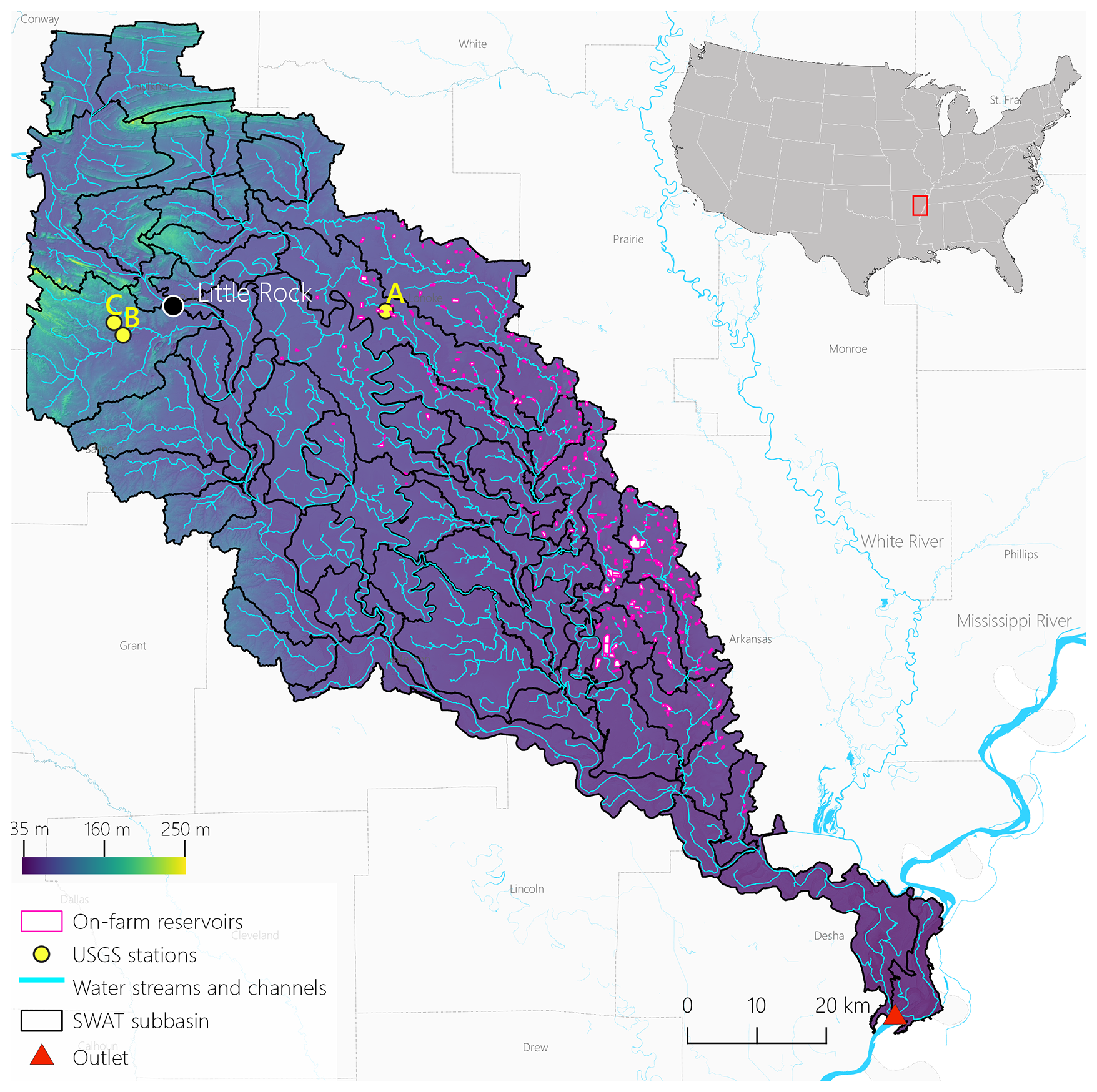
Figure 1 Study region located in eastern Arkansas, USA, the subwatersheds and surface water streams and channels delineated with SWAT+, the model outlet, the United States Geological Survey (USGS) stations (United States Geological Survey Water Data for the Nation, 2022) used for flow calibration and validation, the digitized OFRs (Yaeger et al., 2017), and the Digital Elevation Model (DEM) used in the modeling (Farr et al., 2007).

2.2 SWAT+ model setup

2.2.1 The Soil Water Assessment Tool to model the impacts of OFRs on surface hydrology

The SWAT model is a time-continuous, semi-distributed hydrological model widely used globally – more than 5000 peer-reviewed publications have been published since its launch in the early 1980s (Publications | Soil & Water Assessment Tool (SWAT), 2022). The large number of SWAT applications globally revealed the model development needs and its limitations. To address the present and future challenges when modeling with SWAT, the model source code has undergone significant modifications, and a completely revised version of the model was proposed in SWAT+ (Bieger et al., 2017). SWAT+ utilizes the same equations as SWAT to simulate hydrological processes; however, it provides users with greater flexibility when configuring the model (e.g., defining management schedules, routing constituents, and connecting managed flow systems to the natural stream network) (Bieger et al., 2017).

The SWAT+ is undergoing constant improvements (Chawanda et al., 2020; Molina-Navarro et al., 2018), and a new module (Molina-Navarro et al., 2018) has been recently developed to facilitate the optimal integration of a water body and its drainage area within simulated hydrological processes. In previous versions of the model, when delineating the watershed area draining into a water body, users were required to place an outlet at a specific point in the water stream's network, and areas between the rivers' subwatersheds flowing into the water body were therefore excluded. If these areas are disregarded, critical hydrological processes (e.g., evaporation, overland and/or groundwater flow) flowing into the water body are not accounted for (Molina-Navarro et al., 2018). This former approach can lead to inaccuracies when delineating the watershed areas, mainly when the results are used as input to an OFR model component. The newest versions of SWAT+ consider the OFRs' outline (i.e., shape and surface area) when delineating the watersheds; hence, accounting for the entire drainage area flowing into the waterbody (Molina-Navarro et al., 2018). In addition, the latest versions allow for adding more than one OFR per subwatershed by associating the OFR with channels – components of the watersheds, as well as finer divisions and extensions of water stream reaches, enabling modeling analyses at the channel scale. When simulating the impact of the OFRs at the channel scale, there is a higher level of detail of where and when the OFRs are contributing to changes in surface hydrology, unlike the previous versions of the model, which allowed adding only a single OFR per subwatershed placed at the subwatershed outlet as a point (Arnold et al., 2012), and therefore, the analyses were conducted at the subwatershed scale.

We modeled the impact of OFRs on surface hydrology using the QSWAT+ (v.2.1.9) SWAT+ model interface together with SWAT+ Editor (v.2.1.0) to set up the model, to input the required datasets (e.g., DEM, land use and land cover layer, interpolated meteorological climate information), and to run the different modeling scenarios.

The modeled watershed (710 700 ha, Fig. 1) comprised 68 subwatersheds and a total of 642 Hydrological Response Units (HRUs) – HRUs are unique portions of the subwatersheds characterized by distinct land use and management, as well as unique soil attributes. We set up daily simulations for 30 years (1990–2020), including five years of model warm-up to establish the initial soil water conditions and hydrological processes. The watershed was delineated using the Shuttle Radar Topography Mission DEM (30 m) (Farr et al., 2007). Additionally, we set the channel length threshold to 6 km² and the stream length threshold to 60 km². We placed an outlet in the southern part of the study region – where the lowest part of the watershed is located (Fig. 1). We created the HRUs using the dominant option – this option selects the largest HRU within the subwatershed as the general HRU – within QSWAT+ interface, and used the National Land Cover Database (30 m) (Homer et al., 2020), and Gridded Soil Survey Geographic Database (gSSURGO) (Soil Survey Staff, USDA-NRCS, 2021) (100 m) as inputs to the model. The gSSURGO layers were processed according to their guidelines when using them on QSWAT+ (George, 2020). For climate data, we extracted the centroid coordinates of each subwatershed. We used these centroids to download 30 years of daily precipitation, minimum and maximum temperatures, surface downward shortwave radiation, wind velocity, and relative humidity from the Gridded Surface Meteorological Datasets (Abatzoglou, 2013), which are available in Google Earth Engine (Gorelick et al., 2017). The time series of each subwatershed centroid was added to the SWAT+ Editor as independent weather stations.

2.2.2 Model calibration and validation procedures

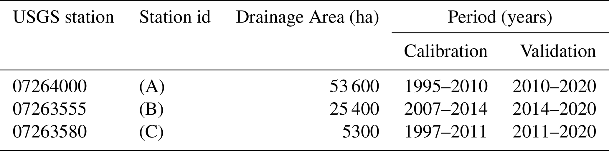
We used monthly measured flow from three USGS stations (Fig. 1 and Table 1) to calibrate and validate the model flow simulations. The USGS flow time series length varied between 14 and 25 years, and we used 60 % of the time series for calibration and 40 % for validation for each USGS station (Table 1). We assessed the performance of the model by calculating the Coefficient of determination (r²), Percent bias (PBIAS, %, Eq. 1) (Yapo et al., 1996), and the Nash–Sutcliffe model efficiency coefficient (NSE, Eq. 2) (Nash and Sutcliffe, 1970). PBIAS is the relative mean difference between the simulated and measured flow values, reflecting the model's ability to simulate monthly flows accurately. The optimal PBIAS is zero, and low-magnitude values indicate better model performance. Positive PBIAS indicates overestimation bias, whereas negative values denote underestimation bias. The NSE indicates how well the model simulates flows, ranging from a negative value to one, with a value of one indicating a perfect fit between the simulated and measured flow values. In general, the model simulations of monthly flow are considered satisfactory when r² ranges from 0.60 to 0.75, PBIAS ranges from ±10 % to ±15 %, and NSE ranges from 0.50 to 0.70 (Moriasi et al., 2015).

Table 1 USGS stations, drainage areas, and the periods used for flow calibration and validation.

$$\begin{array}{}\text{(1)}& {\displaystyle }\mathrm{PBIAS}={\displaystyle \frac{{\sum }_{i=\mathrm{1}}^n(Y_i-X_i)}{{\sum }_{i=\mathrm{1}}^n{X}_i}}\text{(2)}& {\displaystyle }\mathrm{NSE}=\mathrm{1}-{\displaystyle \frac{{\sum }_{i=\mathrm{1}}^n(X_i-Y_i{)}^{\mathrm{2}}}{{\sum }_{i=\mathrm{1}}^n(X_i-\underset{\mathrm{¯}}{X_i}{)}^{\mathrm{2}}}}\end{array}$$

where X_i is the measured flow and Y_i is the simulated flow.

We conducted a sensitivity analysis using the SWAT+ ToolBox (v.0.7.6) (SWAT+ Toolbox, 2022) to reveal the most sensitive parameters when simulating flow – a total of 10 parameters (Table S1) were tested based on previous studies that used SWAT/SWAT+ to model the impact of water impoundments on surface hydrology (Jalowska and Yuan, 2019; Yongbo et al., 2014; Ni et al., 2020; Ni and Parajuli, 2018; Perrin et al., 2012; Rabelo et al., 2021; Zhang et al., 2012). Following the sensitivity analysis, we selected the five most sensitive parameters (Table 2) and proceeded with a manual calibration using the SWAT+ Toolbox. We aimed to improve the model's monthly flow predictions by testing the parameters one at a time and adjusting their values between −20 % and 20 % in 5 % increments, based on their respective ranges. The final calibrated parameters and their fitted values are shown in Table 2.

Table 2 Monthly flow calibration parameters.

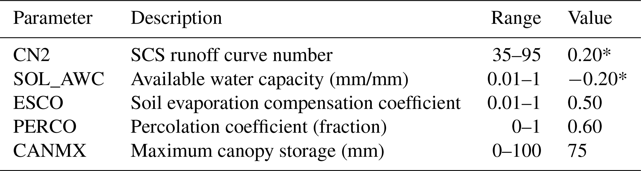
* Denotes relative percentage change.

2.3 OFRs representation in SWAT+

Multiple OFRs can be added to the same subwatershed by associating them with channels (Dile et al., 2022). The OFRs must have at least one outlet channel, and they may have none or multiple inlet channels. Therefore, most OFR-related processes within the model involve determining what channels form inflowing and outflowing channels for each OFR. Ideally, each OFR would interact with a channel, and therefore, have a channel entering, leaving, or within the OFR. Nonetheless, it is common to have OFRs that do not intersect with any channel (Dile et al., 2022) – this is the case for 93 % of the OFRs in our study region. The OFRs in our study region are not dams along the streams but instead engineered water impoundments that are indirectly connected to the main streams via pipes and pumps (Yaeger et al., 2017). A possible solution would be modifying the OFRs' shapes by dragging them to the closest channel (Dile et al., 2022). However, this would require extensive modifications of the OFRs' shapes. Additionally, when an OFR is added to a channel, it is split into two channels, and the model must account for these two newly created channels during the water routing calculations. For this reason, adding multiple OFRs to the same channel or adding multiple OFRs closely located to the same channel can be a cumbersome process that leads to numerous routing errors.

To overcome these challenges, we aggregated the OFRs' surface area and added aggregated OFRs to the model. This adaptation involved two steps. First, for each of the 330 OFRs, we searched for the closest channel by calculating the distance between the OFR's centroid and the multiple channels within each subwatershed. Then, we aggregated all the OFRs associated with each channel by summing their surface areas and adding a polygon representing the aggregated area to the OFR. This approach resulted in 69 aggregated OFRs that were added to 67 different channels located in 16 subwatersheds. The surface area of the aggregated OFRs varied between 3.05 and 165.67 ha, and the number of OFRs in each aggregated OFR varied between 2 and 12. To avoid confusion, for the rest of the manuscript, we refer to OFRs as the aggregated OFRs, and not the individual OFRs shown in Fig. 1.

2.4 OFR's water balance

We did not have access to water abstraction data from the OFRs; therefore, all abstractions were modeled using Eq. (3), which accounts for water flowing out of the OFR, as well as losses due to evaporation and seepage. The volume of water in an OFR, which changes due to changes in inflows, outflows, or abstractions, is associated with changes in the surface area of the OFR. A reduction in surface area (Eq. 4) typically leads to a corresponding decrease in water volume. If inflows are insufficient to fill the OFR, water will not be routed to the downstream channel.

For each of the aggregated OFR, the initial water volume (Vstored, see Eq. 3) was calculated using the SWAT+ default rule, which is a simple multiplication of the OFR surface area by a factor of 10, similar to other studies based on SWAT+ (Ni and Parajuli, 2018; Zhang et al., 2012). For a scenario where the OFR has a surface area of 1 ha (10 000 m²), the corresponding volume would be 100 000 m³ – this is a limitation of our study, as the assumption was necessary due to the absence of available bathymetry data. In addition, since we did not have access to the OFRs' release rates, we used the model's default release rule, which sets the OFRs to release water when the spillway volume is reached – 80 % of the OFRs' capacity (Bieger et al., 2017). While farmers may occasionally withdraw water directly from OFRs, in our study region, most irrigation appropriations are taken from channels and streams. This is consistent with irrigation practices in Arkansas, where large-scale surface water projects withdraw directly from rivers and distribute water via canals and pipelines. Similarly, watershed-scale modeling that incorporates irrigation withdrawals into the river system yields better flow simulations, especially during low-flow periods (Brochet et al., 2024). Given this, and in the absence of high-resolution data on reservoir-specific withdrawals, our framework assumes that inflow to OFRs already reflects upstream irrigation abstractions. Thus, Eq. (3) omits an explicit irrigation withdrawal term for OFRs, and our approach focuses on quantifying the alterations in the hydrological signal through comparisons of natural versus reservoir-influenced flows.

$$\begin{array}{}\text{(3)}& V=V_{\mathrm{stored}}+V_{\mathrm{flowin}}+V_{\mathrm{flowout}}+V_{\mathrm{pcp}}+V_{\mathrm{evap}}+V_{\mathrm{seep}}\end{array}$$

Where V is the volume of water in the OFR at the end of the day (m³), V_stored is the volume of water stored at the beginning of the day (m³), V_flowin is the volume of water entering the OFR during the day (m³), V_flowout is the volume of water flowing out of the OFR (m³), V_pcp is the volume of precipitation falling on the water body (m³), V_evap is the volume of water removed from the OFR due to evaporation, and V_seep is the volume of water lost by seepage (m³).

The OFR surface area is used to calculate the amount of precipitation falling on the water body and the amount of water lost through evaporation and seepage. Given the initial, OFR surface area obtained from one of the three modeling scenarios, the OFR surface area was modeled daily. The surface area varied according to the volume of water stored in the reservoir. Equation (4) is used to estimate the surface area:

$$\begin{array}{}\text{(4)}& {\displaystyle }\text{Surface area }\left(\mathrm{ha}\right)={\mathit{\beta }}_{\mathrm{sa}}+V_{\mathrm{expsa}}\text{(5)}& {\displaystyle }\text{expsa}={\displaystyle \frac{{\log }_{\mathrm{10}}\left(V_{\mathrm{em}}\right)-{\log }_{\mathrm{10}}\left(V_{\mathrm{pr}}\right)}{{\log }_{\mathrm{10}}\left({\text{Surface area}}_{\mathrm{em}}\right)-{\log }_{\mathrm{10}}\left({\text{Surface area}}_{\mathrm{pr}}\right)}}\text{(6)}& {\displaystyle }{\mathit{\beta }}_{\mathrm{sa}}=\left({\displaystyle \frac{V_{\mathrm{em}}}{{\text{Surface area}}_{\mathrm{em}}}}\right)\text{expsa}\end{array}$$

Where βsa is a surface area coefficient, V_em is the volume of water (m³) at the emergency spillway, V_pr is the volume of water (m³) at the principal spillway, Surface areaem is the surface area (ha) at the emergency spillway, and Surface areapr is the surface area at the principal spillway. Spillways release the water once it reaches a specific level. Most OFRs have uncontrolled spillways, implying that there are no gates to control the outflow. The outflow through the spillway depends on the level above the spillway crest. An emergency spillway, whose crest is typically at a higher elevation than the principal spillway, is an additional spillway designed to release excess water during heavy flooding. The surface area of the OFR represents the water spread area corresponding to a given level in the reservoir, which typically increases as the reservoir level rises.

The volume of precipitation falling into the OFR is calculated using Eq. (7):

$$\begin{array}{}\text{(7)}& V_{\mathrm{pcp}}=\mathrm{10}\times R_{\mathrm{day}}\times \text{Surface Area (ha)}\end{array}$$

Where R_day is the amount of precipitation falling into the OFR on a given day (mm).

Evaporation losses are calculated using Eq. (8):

$$\begin{array}{}\text{(8)}& V_{\mathrm{evap}}=\mathrm{10}\times \mathit{\eta }\times E_{\mathrm{0}}\times \text{Surface area (ha)}\end{array}$$

Where η is an evaporation coefficient (0.6), and E₀ is the potential evapotranspiration for a given day (mm).

Seepage losses are calculated using Eq. (9):

$$\begin{array}{}\text{(9)}& V_{\mathrm{seep}}=\mathrm{240}\times K_{\mathrm{sat}}\times \text{Surface area (ha)}\end{array}$$

where K_sat is the effective saturated hydraulic conductivity of the reservoir bottom (mm h⁻¹).

2.5 Scenario Analysis

Given our representation of the OFRs in SWAT+, we assessed the impact of the OFRs on surface hydrology at the channel scale. To do so, we established a model baseline scenario without the presence of OFRs in the watershed. Additionally, we divided the channels into four classes (i.e., low and high flow classes) based on their mean baseline flow. The different class intervals were calculated using the mean flow quartiles, accounting for all channels, which resulted in the following baseline flow classes: (1) 0.001–0.25 m³ s⁻¹, (2) 0.25–0.50 m³ s⁻¹, (3) 0.50–2.11 m³ s⁻¹, and (4) 2.11–17.50 m³ s⁻¹.

To account for the OFRs' variation in surface area (i.e., change in storage capacity), we propose a novel approach that leverages a top-down data-driven model based on satellite imagery (Fig. 2). We used this model to create three modeling scenarios using daily OFRs surface area time series – these scenarios were based on the methodology proposed by Perin et al. (2022). The authors employed a multi-sensor satellite imagery approach combined with the Kalman filter (Kalman, 1960) to calculate the daily OFRs' surface area change between 2017 and 2020. The proposed algorithm accounts for the uncertainties in both the sensor's observations and the resulting surface areas. By improving the OFR's surface area observations cadence, the algorithm enables a deeper understanding of the OFR's surface area intra- and inter-annual changes, which are key pieces of information that can be used to better assess and manage the water stored by the OFR (Perin et al., 2022). The daily surface area time series – derived by combining PlanetScope, RapidEye, and Sentinel-2 satellite imagery (Perin et al., 2022) – of each OFR was used to simulate three scenarios (i.e., lower, mean, and upper) representing the OFRs' capacity in terms of surface area. The mean scenario represents the regular condition of the OFRs, and it is the mean of the daily surface area time series derived from the Kalman filter. The lower and upper scenarios represent the lowest and highest capacities of the OFRs, based on the 95 % confidence interval limits of the surface area, calculated using the daily time series. Please refer to Perin et al. (2022) for more details on how the 95 % confidence interval was calculated.

The SWAT+ model does not allow for direct incorporation of a daily surface area time series because it calculates surface area dynamically (Eq. 4) based on changes in water volume through the reservoir water balance equation (Eq. 3). It is structured to accept a single surface area value per scenario, which then varies internally. Incorporating time-varying surface area data, such as from the Kalman filter, would require modifications to the model that are currently not supported. Therefore, a single surface area value was assigned to each scenario and OFR, with lower, mean, and upper values used as starting points for the model's water balance simulations. This initial surface area reflects the OFR's maximum surface area at full capacity for each scenario. For example, in the lower scenario, an initial surface area of 1.2 ha represents the maximum area for this OFR. As model iterations proceed, the surface area is recalculated based on Eq. (4). The initial OFR surface area was kept constant during the simulation period (Ni et al., 2020; Ni and Parajuli, 2018; Perrin et al., 2012). In other words, the OFR surface area varied according to Eq. (4), however, the maximum surface area did not exceed the initial value. To assess the impact of the OFRs on surface hydrology, we compared the baseline flow with the flow simulated by each surface area scenario – i.e., comparing the flow changes with and without OFRs, a common approach used by previous studies (Habets et al., 2018).

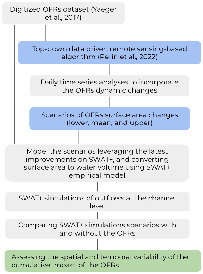
Figure 2 A new approach to integrate a top-down data-driven remote sensing-based algorithm, that assesses the OFR's dynamic conditions (Perin et al., 2022), with the latest SWAT+ model developments.

We estimated the impact of the OFRs on surface hydrology by calculating the percent change (Eq. 10) of monthly flow between the baseline and the three surface area scenarios, including all OFRs. The annual impact on flow was calculated by averaging the mean percent change over the months. We also calculated the distribution of the percent change for each baseline flow class. The distribution was assessed using two-dimensional kernel density estimation (KDE) plots. Unlike discrete bins (e.g., histograms), KDE plots display a continuous density estimate of the observations using a Gaussian kernel. Additionally, we assessed the percentage changes in peak flow. For this analysis, peak flow is defined as equal to or higher than the 99th flow percentile calculated using the entire flow time series (Eq. 10). It is important to keep in mind that the impact of the OFRs on this study is solely based on modeling scenarios and does not account for OFR management practices, which represents a key limitation of this simulation study.

$$\begin{array}{}\text{(10)}& \text{Percent change }\left(\mathit{\%}\right)=\left({\displaystyle \frac{Y_i-X_i}{X_i}}\right)\times \mathrm{100}\end{array}$$

Where X_i is the baseline flow, and Y_i is the simulated flow of each surface area scenario.

3 Results

3.1 Model calibration and validation

The model calibration and validation were done using the three USGS stations presented in Fig. 1 and Table 1, and accounting for all OFRs in the study region. When comparing the monthly simulated flow with the measured flow for the calibration period, there was a good agreement (0.71 r² 0.93), and a satisfactory model efficiency (0.68 NSE 0.90) for all three stations (Fig. 3). In addition, the PBIAS magnitude was <3 % for station A, and <12 % for stations B and C. Meanwhile, the validation period had r² ranging between 0.69 and 0.86, and the NSE between 0.68 and 0.83, with PBIAS magnitude <10 % for stations A and B, and 18.12 % for station C. In general, for stations A and C, the model overestimated flow values (i.e., positive PBIAS) mostly during flow events <3 m³ s⁻¹, and the model underestimated flow (i.e., negative PBIAS) for station B during flows >20 m³ s⁻¹ (Fig. 3). These findings are consistent with a previous study conducted in western Mississippi near our study region (Ni and Parajuli, 2018). Even though during the validation period, Station B had a PBIAS magnitude higher than 15 %, the r² and NSE values from both the calibration and validation periods indicate satisfactory modeling performance when simulating monthly flow (Moriasi et al., 2015). Given that none of the OFRs were directly connected with the streams where the stations were located (Fig. 1), and there were no OFRs near stations B and C, the calibration and validation metrics with and without the OFRs were very similar, with differences smaller than 1 %.

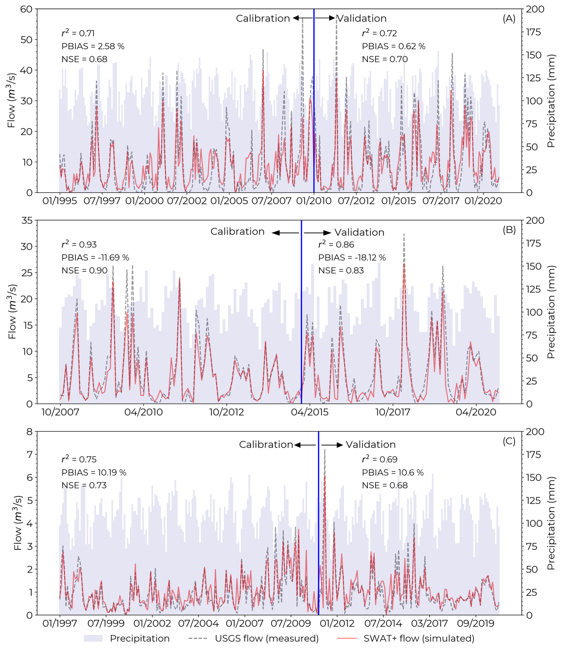
Figure 3 Flow calibration and validation time series for the three USGS stations A (07264000), B (07263555), and C (07263580). See Fig. 1 and Table 1 for more information about the USGS stations. The precipitation time series represents the monthly accumulated precipitation at the watershed scale (i.e., for the entire study region).

3.2 Percent change in flow

We assessed the impact of the OFRs on flow by comparing the baseline flow (i.e., without the OFRs) with the three surface area scenarios generated from the Kalman filter approach – lower, mean, and upper (see Sect. 2.4, and Fig. 2). The total surface area (i.e., summing all OFRs surface area) was 2.176 ha for the lower, 2.766 ha for the mean, and 3.370 ha for the upper, and the three scenarios had a similar OFRs surface area distribution (Fig. 4). In addition, most of the OFRs had surface areas <50 ha – 78 %, 71 %, and 62 % of the OFRs for the lower, mean, and upper scenarios.

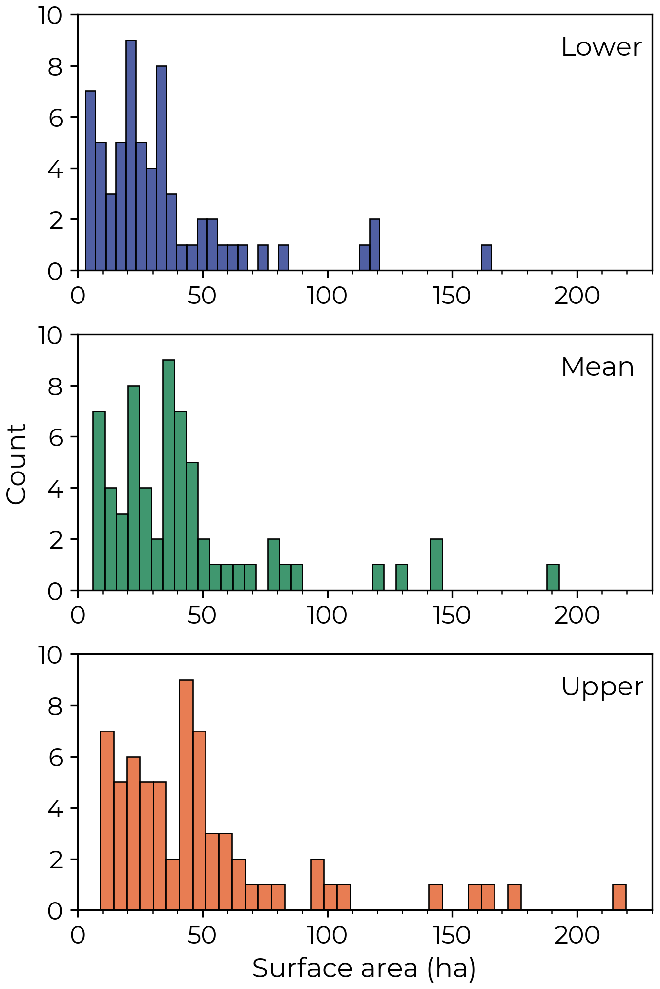
Figure 4 OFR's surface area distribution for the three surface area scenarios, lower, mean, and upper.

Figure 5 categorizes the channels into four distinct groups, with each category illustrating the percentage change in flow throughout the year, displayed along the x axis by month. The three bar colors represent different scenarios, while bar heights illustrate variations across channels and years. For example, the bars for January include all January data spanning from 1990 to 2020, enabling a thorough comparison of seasonal and year-to-year flow changes. The impact of the OFRs on monthly flow varied throughout the year. The largest impacts occurred between January and May for all flow classes (Fig. 5). During these months, including all surface area scenarios, the mean decrease in flow (i.e., negative mean percent change) was $-\mathrm{34.4}\pm \mathrm{6}$ % for class 1, $-\mathrm{37.6}\pm \mathrm{5}$ % for class 2, $-\mathrm{30.0}\pm \mathrm{6}$ % for class 3, and $-\mathrm{34.1}\pm \mathrm{6}$ % for class 4. For all classes, the most significant reduction in flow occurred during March ($\sim -\mathrm{40}$ %). Meanwhile, the impact of the OFRs was more minor during the second half of the year, in which the mean percent change in flow was $-\mathrm{12.0}\pm \mathrm{3}$ % for class 1, $-\mathrm{12.5}\pm \mathrm{5}$ % for class 2, $-\mathrm{1.4}\pm \mathrm{4}$ % for class 3, and $-\mathrm{2.6}\pm \mathrm{10}$ % for class 4 (Fig. 5).

When assessing the mean percent change per month for all surface area scenarios, the lower flow classes (i.e., (1) 0.001–0.25 m³ s⁻¹ and (2) 0.25–0.50 m³ s⁻¹) exhibited a negative mean percent change for all months. Nonetheless, we observed a mean positive percent change (i.e., increase in flow) for August (5.0±1 %) and October (5.2±0.2 %) for class 3, and during June (8.2±0.3 %), August (7.3±0.4 %), and October (8.7±0.4 %) for class 4 (Fig. 5). Furthermore, the different surface area scenarios had similar impacts on flow for all months of the year with differences smaller than 5 % for all scenarios. Between January and May, for all flow classes, the mean percent change was $-\mathrm{32.0}\pm \mathrm{6}$ % for the lower, $-\mathrm{34.6}\pm \mathrm{7}$ % for the mean, and $-\mathrm{35.8}\pm \mathrm{5}$ % for the upper. Between June and December, the impact on flow was $-\mathrm{5.4}\pm \mathrm{6}$ % for the lower, $-\mathrm{7.3}\pm \mathrm{8}$ % for the mean, and $-\mathrm{8.9}\pm \mathrm{5}$ % for the upper.

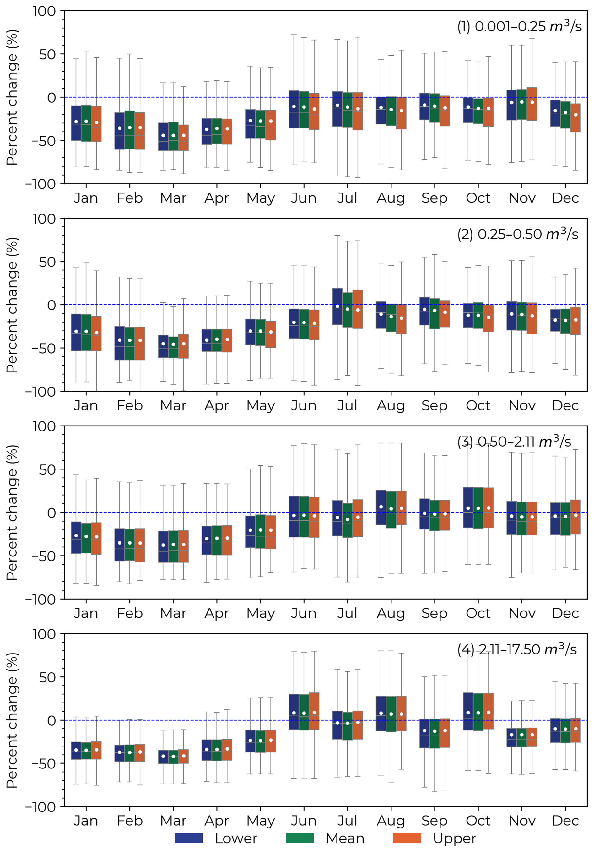
Figure 5 Monthly percent change in flow between the baseline scenario (vertical dotted blue line) and the three surface area scenarios (lower, mean, and upper), and for the four flow classes (1) 0.001–0.25 m³ s⁻¹, (2) 0.25–0.50 m³ s⁻¹, (3) 0.50–2.11 m³ s⁻¹, and (4) 2.11–17.50 m³ s⁻¹. This analysis included data from all simulated years (1990–2020).

Generally, the OFRs contributed to a decrease in monthly flow. However, the OFRs' impact on flow exhibited significant intra- and inter-annual variability, varying according to different OFRs and channels – this is highlighted by the boxplot size variability in Fig. 5, where the variability was lower during the first part of the year and greater between July and August. Additionally, the monthly percent change in flow in the KDE plots (Fig. 6) indicates that for all three scenarios and flow classes, most changes in flow fall within the range of −40 % to 0 %. In addition, all KDE plots have a triangular shape with its base on the smaller flows, denoting where most of the changes occur. Even though most of the percent change in flow is negative, there are circumstances in which the OFRs could positively impact flow – the increase in flow is represented by faded colors in each surface area scenario (Fig. 6). The positive mean percent change could be as high as 80 % – see Fig. 6 for the larger flow classes, (3) 0.50–2.11 m³ s⁻¹ and (4) 2.11–17.50 m³ s⁻¹. The positive impact on flow for these classes was observed during June, August, and October, when a mean positive change was noted (Fig. 5, classes 3 and 4).

The annual mean percent change, for all surface area scenarios, was $-\mathrm{22.5}\pm \mathrm{3}$ % for class 1, $-\mathrm{24.2}\pm \mathrm{4}$ % for class 2, $-\mathrm{14.6}\pm \mathrm{3}$ % for class 3, and $-\mathrm{16.6}\pm \mathrm{3}$ % for class 4. In addition, the surface area scenarios' annual changes were $-\mathrm{18.0}\pm \mathrm{5}$ % for the lower, $-\mathrm{19.6}\pm \mathrm{5}$ % for the mean, and $-\mathrm{20.8}\pm \mathrm{6}$ % for the upper, including all flow classes. The differences between the surface area scenarios shown in Figs. 5 and 6 are related to the variability of the OFR's surface area.

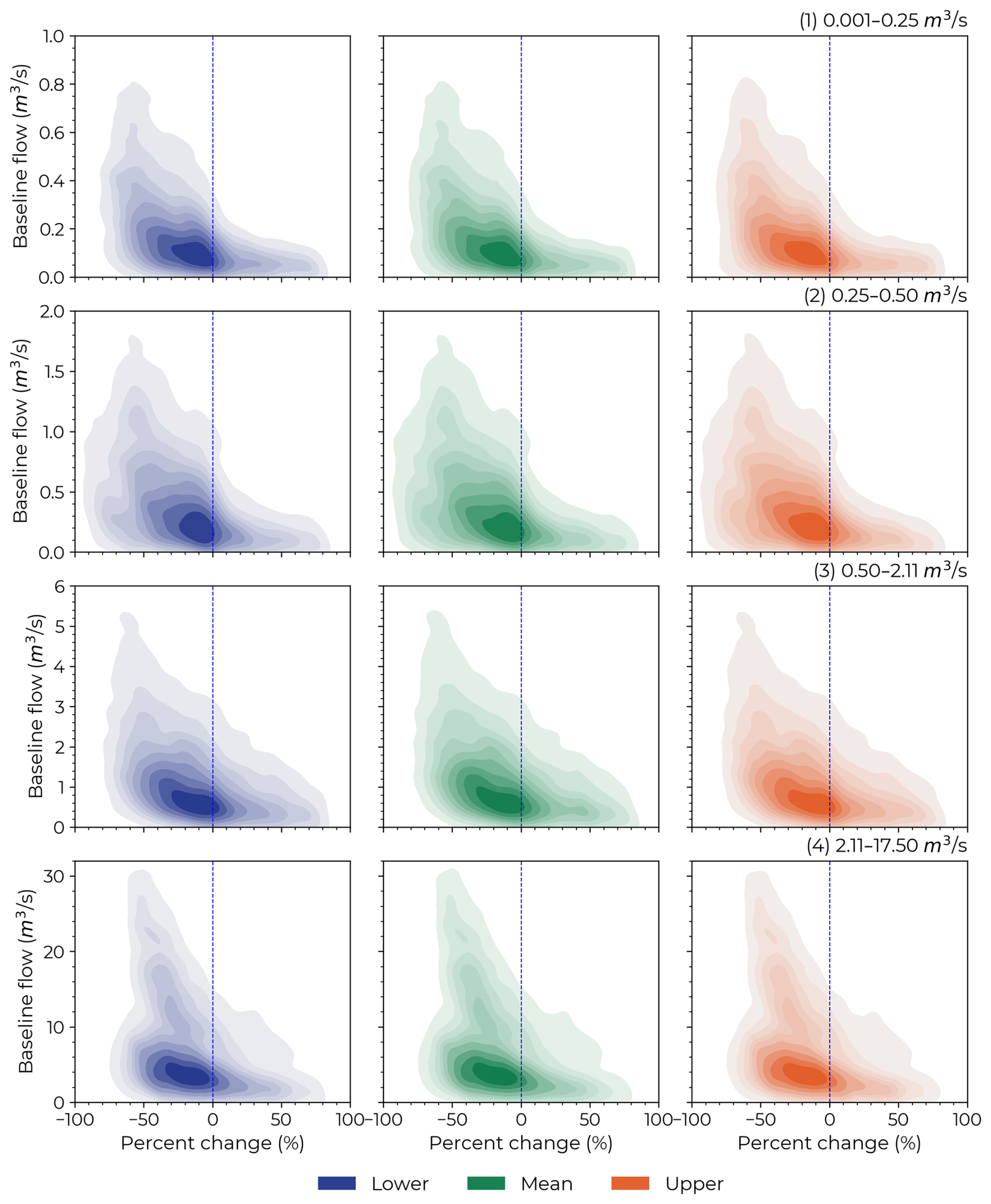
Figure 6 Kernel density estimation plots smoothed using a Gaussian kernel for the monthly percent change in flow between the baseline scenario (vertical dotted blue line) and the three surface area scenarios (lower, mean, and upper) for the four flow classes (1) 0.001–0.25 m³ s⁻¹, (2) 0.25–0.50 m³ s⁻¹, (3) 0.50–2.11 m³ s⁻¹, and (4) 2.11–17.50 m³ s⁻¹. Note the different range of values on the y axis for all four flow classes.

3.3 Impact on peak flow

For each channel, we calculated the impact of the OFRs on peak flow (Fig. 7). The effect on peak flow was $-\mathrm{60.7}\pm \mathrm{13}$ % for class 1, $-\mathrm{56.2}\pm \mathrm{11}$ % for class 2, $-\mathrm{46.7}\pm \mathrm{19}$ % for class 3, and $-\mathrm{43.9}\pm \mathrm{12}$ % class 4. When assessing the impact on peak flow based on different surface area scenarios, the mean percent change was $-\mathrm{49.4}\pm \mathrm{18}$ % for the lower, $-\mathrm{50.4}\pm \mathrm{17}$ % for the mean, and $-\mathrm{52.7}\pm \mathrm{18}$ % for the upper. All peak flows occurred between January and May, which is the period of the year when the study region receives most of its precipitation (Perin et al., 2021a). Except for a few outliers, there was no increase in peak flow, despite the OFRs contributing to a positive mean percent change in flow in certain months of the year (Fig. 5, classes 3 and 4).

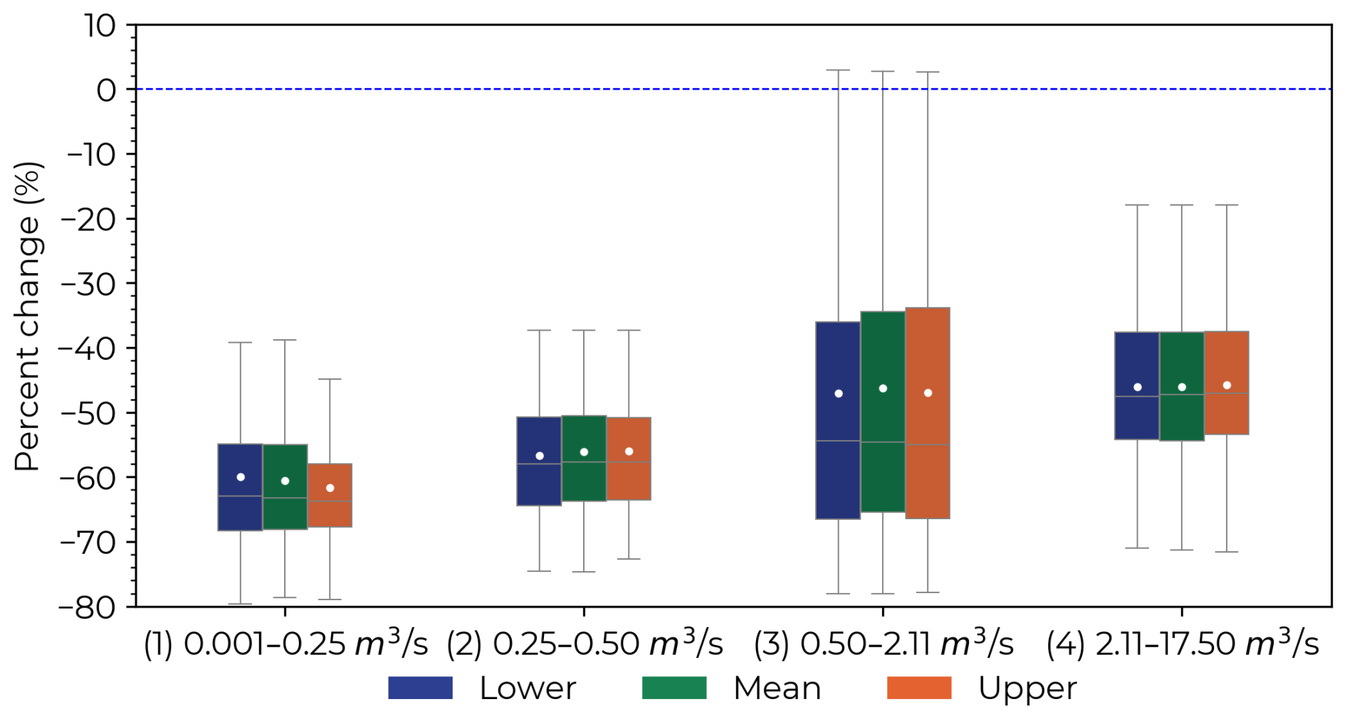
Figure 7 Percent change in peak flow between the baseline scenario (vertical dotted blue line) and the three surface area scenarios (lower, mean, and upper) for the four flow classes (1) 0.001–0.25 m³ s⁻¹, (2) 0.25–0.50 m³ s⁻¹, (3) 0.50–2.11 m³ s⁻¹, and (4) 2.11–17.50 m³ s⁻¹.

3.4 Simulated flow time series

We randomly selected a channel within the flow class 3 to demonstrate the baseline and the three surface area scenarios' flow time series between 1995 and 2005 (Fig. 8). For this channel, the annual mean percent changes in flow when comparing the baseline scenario with the lower, mean, and upper surface area scenarios were 0.99±11.8 %, $-\mathrm{1.9}\pm \mathrm{13}$ %, and $-\mathrm{2.0}\pm \mathrm{19}$ % – the high standard deviation for the three scenarios is explained by the interannual variability. The upper surface area scenario resulted in lower flows (i.e., higher impact) compared to the lower and mean scenarios for the majority of flow events – 67.8 % and 57.6 % for the lower and mean scenarios, respectively. Nonetheless, there are circumstances when the upper scenario yielded higher flows – 32.2 % and 42.4 % of the events for the lower and mean scenarios, respectively (e.g., see the two insets for the periods March 1997–August 1998 and May 2002–February 2004). These findings indicate that the impacts that the OFRs have on flow are not entirely governed by the presence and surface area of the OFRs (i.e., the different surface area scenarios), but instead by a combination of the OFRs with varying components of modeling (e.g., terrain, land use, climate information), and different hydrological processes (e.g., run-off, precipitation, evaporation). In addition, the impact on peak flow for this channel was $-\mathrm{45.7}\pm \mathrm{19.7}$ % for all surface area scenarios, as highlighted on two occasions (August 2002 and August 2003) in the second inset.

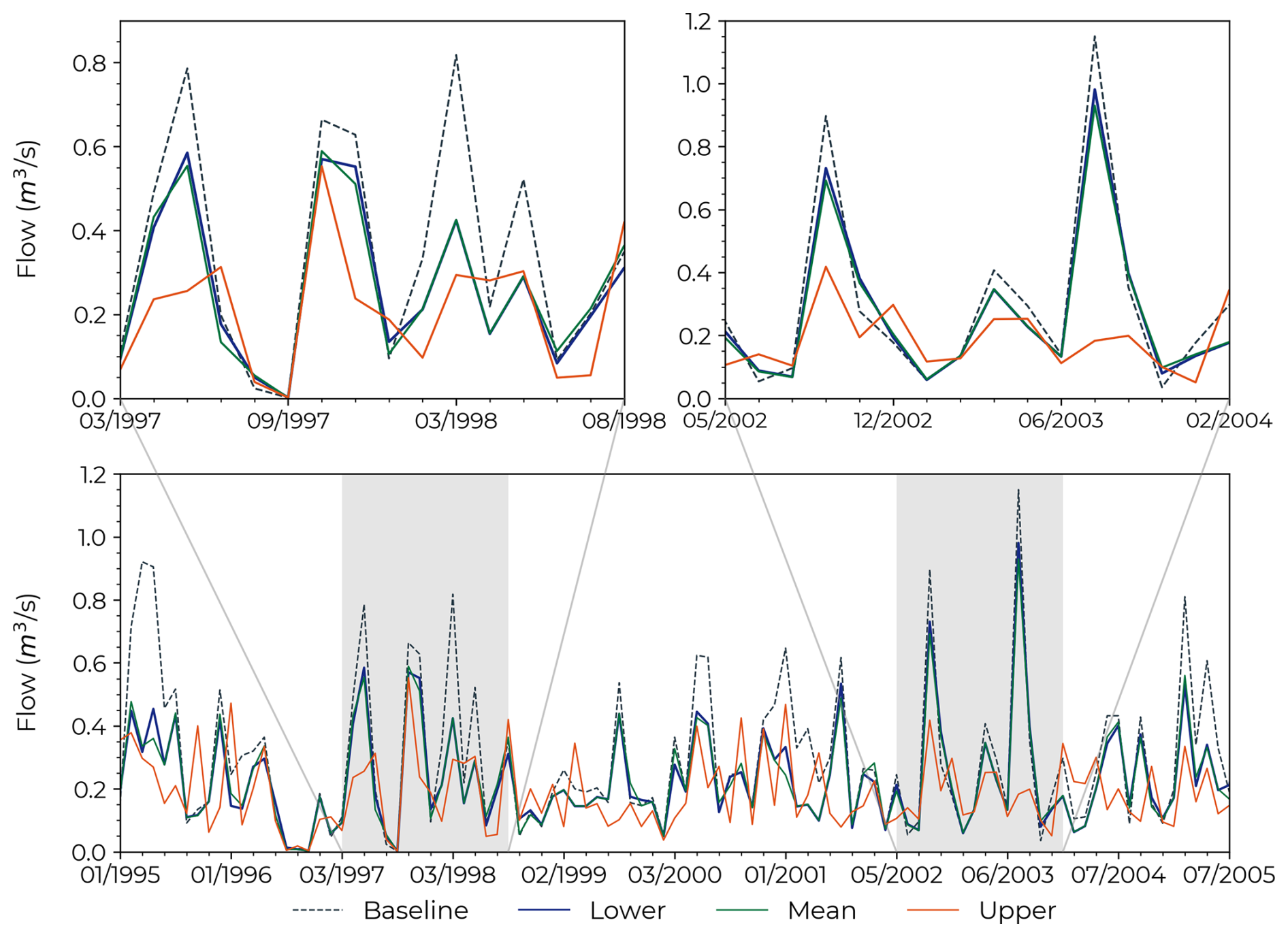
Figure 8 A subset of the time series of simulated flow for baseline and the three surface area scenarios (lower, mean, and upper) between 1995 and 2005 for a selected channel within the flow class 3.

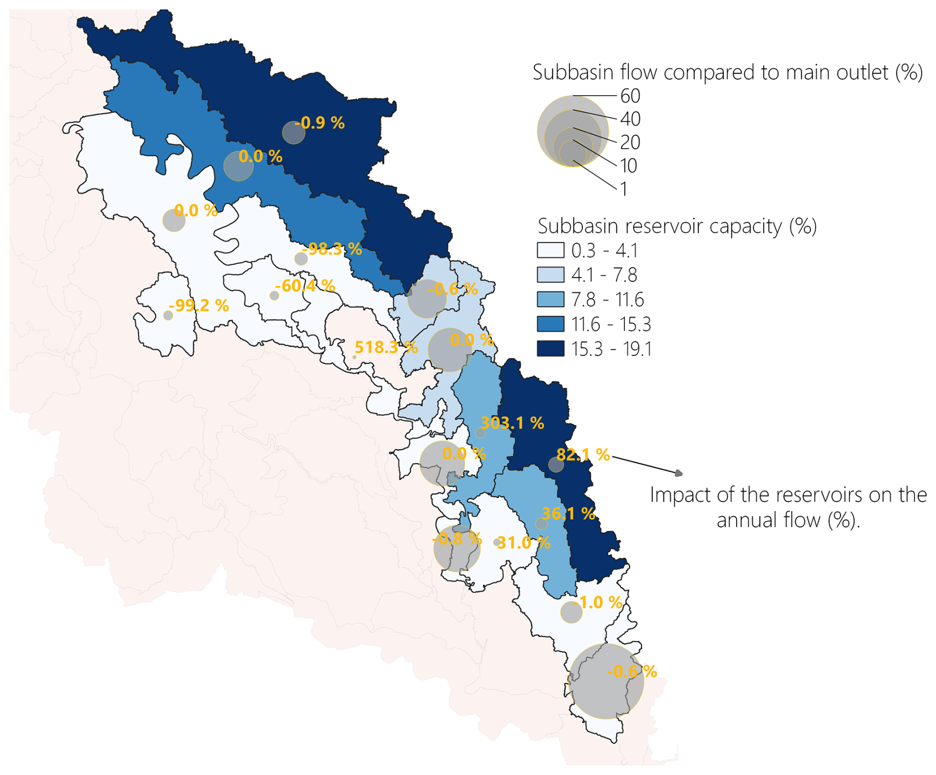
Figure 9 The cumulative impact of OFRs on annual flow for the mean scenario at the subwatersheds where the OFRs occurred. The size of the circles represents the contribution (%) of the subwatershed flow compared to the main outlet (i.e., model outlet). The subwatersheds are color-coded according to their reservoir capacity (%), which was calculated by summing the OFRs surface area in each subwatershed and dividing the sum by the total OFRs surface area (i.e., including all OFRs from all subwatersheds), with a darker color indicating a higher reservoir capacity. The percentages highlighted in yellow represent the impact of the OFRs on annual flow.

3.5 Spatial variability of the OFR's impact on annual flow

To assess the overall impact of the OFRs at the subwatershed level, we calculated the contribution of each subwatershed flow to the main model outlet, and the subwatersheds' reservoir capacity (i.e., summing the OFRs surface area at each subwatershed and dividing it to the total OFRs surface area, including all OFRs from all subwatersheds) (Fig. 9). In general, the highest impacts on annual flow (e.g., >100 %), with positive or negative magnitude, occurred at the subwatersheds that contributed the least (<10 %) to the main model outlet – these subwatersheds are represented in lighter shades of blue, and the annual impact is highlighted in yellow on Fig. 9. In other words, the highest impacts on flow occurred on the channels with smaller flow magnitudes (e.g., channels that presented mean flow ranging between 0.001–0.25 and 0.25–0.50 m³ s⁻¹, these channels were classified as class 1 and 2 in this study). In addition, the subwatersheds with the highest reservoir capacities (between 15.3 % and 19.1 %, represented in darker shades of blue) (Fig. 9) had a small (< 10 %) contribution to the model outlet. These subwatersheds did not present the highest impact on annual flow (e.g., the effect on annual flow for the top two subwatersheds in terms of reservoir capacity were −0.9 % and 82.1 %).

4 Discussion

As OFRs will contribute to improving food production resilience by providing surface water for irrigation during dry periods and severe drought events, which are expected to occur more frequently due to climate change, OFRs can have cumulative impacts on the surface hydrology of the watershed where they are located. Studies have employed either data-driven or physically based hydrological model approaches to estimate the effects of OFRs on watersheds. However, combining these approaches provides a better understanding of the spatial and temporal variability of OFR impacts, as it incorporates the dynamic changes of OFRs into the hydrological model. To quantify whether the impact of the OFRS on mean and peak flow varies intra- and inter-annually, and which subwatersheds are more affected, we combined a data-driven remote sensing-based model with the latest improvements in SWAT+ to assess the OFR impacts.

4.1 Cumulative impact of OFRs

When simulating water impoundments in SWAT/SWAT+, it is common practice to validate and calibrate the model using flow measurements (Evenson et al., 2018; Habets et al., 2018; Jalowska and Yuan, 2019; Ni and Parajuli, 2018). In addition, other studies have validated and calibrated the model using alternative variables. For example, Perrin et al. (2012) employed monthly measurements of piezometric variations to assess aquifer recharge processes, and Jalowska and Yuan (2019) used sediment loadings (concentration and budget) from field monitoring reports to evaluate sediment simulations. Ideally, we would calibrate and validate the model by accounting for the parameters governing the OFRs' water budget (e.g., inflows and outflows) (e.g., Kim and Parajuli, 2014). Nonetheless, these measurements were not available for the OFRs in our study region. Furthermore, a thorough calibration and validation of the model would require extra flow data, covering other parts of the study region, as the three USGS stations – the only data available – used in this study are located in the upper part of the modeled watershed. Similar to Evenson et al. (2018), who proposed a module to better represent spatially distributed wetlands and validated their model using both direct (i.e., flow measurement) and indirect (i.e., wetlands surface area) approaches, our validation and calibration were conducted using flow measurements. The OFR's surface area scenarios were based on an algorithm that was validated with an independent higher spatial resolution dataset (Perin et al., 2022).

There is a consensus within the scientific community that the OFRs will have a cumulative impact on surface hydrology, resulting in decreased flow and peak flow. For example, previous studies have found that OFRs reduce annual and monthly runoffs in southeastern China (Yan et al. 2023) and Australia's Murray-Darling Basin (Robertson et al., 2023). The effect will vary from watershed to watershed due to the number of OFRs and the OFRs' different purposes (e.g., different irrigation schedules) (Ayalew et al., 2017; Fowler et al., 2015; Habets et al., 2018; Nathan and Lowe, 2012; Pinhati et al., 2020; Rabelo et al., 2021). As pointed out by Habets et al. (2018), the mean annual decrease in flow from all studies was $-\mathrm{13.4}\pm \mathrm{8}$ %. Our results align with this value, which varied between $-\mathrm{24.2}\pm \mathrm{4}$ % and $-\mathrm{14.6}\pm \mathrm{3}$ % for all flow classes. In addition, OFRs can reduce peak flow on average by 45 % (Habets et al., 2018; Nathan and Lowe, 2012; Thompson, 2012), and up to 70 % (Ayalew et al., 2017) for certain flow events. Likewise, our results are consistent with these findings, which show a mean impact on peak flow ranging from $-\mathrm{60.7}\pm \mathrm{12}$ % to $-\mathrm{43.9}\pm \mathrm{12}$ %. Furthermore, unlike previous research, our results indicate that the OFRs may have a positive (<9 %) impact on flow (Fig. 5, classes 3 and 4). This can be attributed to the level of detail in our analyses. When evaluating flow changes at the channel scale, it is important to note that flow at this level is several orders of magnitude smaller than at the main basin outlet. Consequently, this scale often exhibits more significant percentage changes, both increases and decreases. This likely explains how OFRs can enhance channel flow, primarily due to the additional water contributed by OFRs, influenced by periods of increased precipitation in certain channels during specific months and years. While we calculated the monthly impact on flow at the channel scale by aggregating the OFRs to the closest channel, previous studies have mainly reported the annual impact on flows (Habets et al., 2018). They performed their analysis at the subwatershed scale by aggregating the OFRs to a single point at the outlet of each subwatershed in SWAT (Evenson et al., 2018; Kim and Parajuli, 2014; Perrin et al., 2012; Zhang et al., 2012), or they used different modeling approaches (see Habets et al., 2018).

By leveraging the latest improvements in SWAT+ to simulate water impoundments (Molina-Navarro et al., 2018) and combining them with a novel algorithm based on time series of satellite data to monitor OFRs (Perin et al., 2022), we modeled the impact of OFRs on flow at the channel scale. In addition, the surface area scenarios enabled us to account for events when the OFRs were at the lowest, regular, and fullest capacities according to their surface area (see Fig. 2). This is an improvement over previous studies (e.g., Ni et al., 2020; Ni and Parajuli, 2018; Perrin et al., 2012) that used a single surface area (i.e., one snapshot in time) to represent the OFRs in SWAT. The small differences (<5 %) between the surface area scenarios in terms of mean percent change in monthly flow indicate that the OFRs' surface area variation had a minimal impact on flow. For instance, during January and May, the mean monthly percent change ranged between $-\mathrm{35.8}\pm \mathrm{6}$ % and $-\mathrm{32.0}\pm \mathrm{7}$ %, and during June and December, it varied between $-\mathrm{8.8}\pm \mathrm{5}$ % and $-\mathrm{5.4}\pm \mathrm{6}$ % for the three surface area scenarios. The same was observed for peak flow, with a mean monthly impact ranging between $-\mathrm{52.7}\pm \mathrm{17}$ % and $-\mathrm{49.4}\pm \mathrm{18}$ %. This small variability on flow impact was observed even though the total OFR surface area increased by 590 and 1194 ha when comparing the lower scenario with the mean and upper scenarios (Fig. 5). However, the OFRs represented a small portion (<1 %) of the total area of the modeled watershed (Fig. 1). These findings are related to the fact that flow simulations are governed by several hydrological processes (e.g., run-off, precipitation, evapotranspiration) besides the presence of OFRs on the channel (Bieger et al., 2017; Dile et al., 2022; Arnold et al., 2012). In addition, when assessing the percent change in flow at the channel scale, the differences in surface area between the scenarios were of a lower magnitude compared to the total OFR's surface area. For instance, an OFR with a surface area smaller than 10 ha, and with surface area variations between 10 % and 20 % for the three scenarios, may not lead to significant differences (e.g., >10 %) between the three scenarios.

4.2 OFRs' impacts on flow and peak flow

Our findings highlight that the impacts of the OFRs on flow and peak flow have a significant intra- and inter-annual variability (Figs. 5, 6, and 7). The impacts vary according to different OFRs and channels (Fig. 5). The most significant impacts on flow occurred during the first part of the year, between January and May, a period when peak flows typically occur. In addition, this time of the year also coincides with the period when the region receives most of its precipitation (Perin et al., 2021b), and the OFRs are at their fullest capacity (i.e., OFRs storing their maximum amount of water) (Perin et al., 2022). During the second part of the year, we observed a milder mean percent change in flow for all flow classes and all scenarios, and a greater variability in percent change, notably for July and August (Fig. 5). Moreover, most of the irrigation activities happen between June and September (Perin et al., 2021b, Yaeger et al., 2017). It is when the OFRs are at their lowest capacities (i.e., storing less water) (Perin et al., 2022), which could explain their moderate impact and higher variability during these months, even though we are not accounting for the OFRs' inflows and outflows, and not simulating irrigation events.

Additionally, the variability of the OFRs' impacts is related to the OFRs' physical properties (e.g., surface area and location in the watershed). For example, the OFR surface area will have an impact on flow and peak flow, as shown by the different surface area scenarios, and depending on where the OFR is located in the watershed, given that it may be connected to lower or higher flow channels, which contributes to their impact variability during the year (Figs. 4 and 5). Besides the OFRs' physical properties, the built-in complexity of SWAT – when simulating the presence of the OFRs and the various hydrological processes (e.g., run-off, precipitation, evapotranspiration) governing the water cycle – contributes to the differences in the OFRs' impacts. This complexity is illustrated in Fig. 8, which shows that the upper scenario can have a higher or lower impact on flow compared to the lower and mean scenarios.

When assessing the annual impact of the OFRs accounting for each subwatershed flow compared to the main model outlet flow, and each subwatershed reservoir capacity (Fig. 9), we found that even though the presence of the OFRs can have a significant impact on flow (Figs. 5, 6, and 7), the highest impacts tend to occur on the subwatersheds that contribute the least (<10 %) to the main model outlet. In general, the highest impacts occurred on the channels with smaller flow magnitudes, and the subwatersheds with the highest reservoir capacities did not have the highest impact on flow. The changes in the OFRs' impacts along the year, and between different years, are directly related to the OFRs' water balance (Eq. 3). The variations are primarily driven by the volume of water stored by the OFRs, which is modeled at a daily scale, and it varies according to total daily precipitation, evaporation, and seepage losses.

4.3 Research implications and applications to other study regions

Overall, we presented a new approach to quantitatively analyze the impact of a network of OFRs on mean and peak flow, and we described the various potential reasons behind the variability of the effects of OFRs. Our results indicate that OFRs have an uneven impact on mean and peak flow across the watershed. This variability is primarily influenced by differences in the size, water storage capacity, and the spatial distribution (i.e., their presence) of OFRs. Hence, assessing the OFR's location as well as their numbers across the watershed is important when aiming to manage the construction of new OFRs. In particular, the geospatial variability of the OFRs impacts could be taken into account by water agencies when planning and developing a network of OFRs, given it is possible to identify the areas that are under high pressure (e.g., regions with multiple OFRs that are having a significant impact on flow), and to identify areas that could benefit from the construction of new OFRs, targeting improvements on water resources management and irrigation activities.

Furthermore, even though the OFR's impacts may vary significantly in different watersheds (Habets et al., 2018), our approach could be transferable to other places across the world, as it integrates a top-down data-driven remote sensing-based algorithm, which is based on freely available and private Earth Observations datasets, with the latest SWAT+ hydrological modeling developments. In addition, the widespread use of SWAT+ and its open-source nature are yet another factor contributing to the transferability of the novel approach presented in this study. This is relevant as the number of OFRs is expected to increase globally (Althoff et al., 2020; Habets et al., 2014; Habets et al., 2018; Krol et al., 2011; Rodrigues et al., 2012), with limited knowledge of how the OFRs may impact surface hydrology in different watersheds, and under diverse environmental conditions. Finally, in tandem with the OFRs' key role in irrigated food production, in part to adapt to climate change (Habets et al., 2018) and to alleviate the pressure on surface and groundwater resources (Vanthof and Kelly, 2019; Yaeger et al., 2017, 2018), their impacts on surface hydrology need to be considered to avoid exacerbating the surface water stress already intensified by climate change and population growth (Vörösmarty et al., 2010).

5 Future improvements

Future improvements should focus on how to better represent OFR's water management (i.e., OFR's inflows and outflows) in SWAT+. Given that each OFR has an independent water balance, accounting for the OFR's water volume change would be a more realistic representation of the OFR when compared to the three surface area scenarios tested in this study. Estimating the OFR's volume change can be done by combining the OFR surface area time series with area-elevation equations – these equations describe the OFR's bathymetry, and allow volume estimation by inputting the OFR's surface area (Liebe et al., 2005; Meigh, 1995; Sawunyama et al., 2006). After carefully assessing different methods to derive these equations (Arvor et al., 2018; Avisse et al., 2017; Li et al., 2021; Meigh, 1995; Sawunyama et al., 2006; Vanthof and Kelly, 2019; Yao et al., 2018; Zhang et al., 2016), we concluded that measured ground data of the OFRs' depth – which is not available – is required to estimate the equations with an acceptable uncertainty. Estimating the area-elevation equations entails several challenges, including: (1) even though there are several DEMs available for the study region (Arkansas GIS Office, 2022) – DEMs can be used to estimate the OFRs bottom elevation – the DEMs were collected when most of the OFRs were full (i.e., bathymetry was not exposed), which limits their use in this case; and (2) although the OFRs are located within the same geomorphological region, they have different depth, shape and physical characteristics (Perin et al., 2022; Yaeger et al., 2017). Therefore, even if a generalized area-elevation equation were calculated for our study region – this is a common approach employed by other studies (Mady et al., 2020; Vanthof and Kelly, 2019) – that would still lead to high uncertainties in water volume changes. Ideally, each OFR would have its own equation, which was not possible when this study was done. Future work should integrate data on actual evapotranspiration, ET (Kiptala et al., 2014) to quantify as the balance between water availability and ET determines in large part the irrigation system efficiency and crop productivity in the watersheds where OFRs occur.

Efforts should also be made to improve SWAT+ capabilities to receive measured OFRs' inflows and outflows. The latest version of the model has improved the hydrological representation of small water impoundments in SWAT+ (Molina-Navarro et al., 2018). Nonetheless, at the time of our study, the newest version of the model does not allow users to input measured or calculated OFRs' inflows and outflows. Instead, the model developers recommend simulating the OFR's water balance using decision tables (Arnold et al., 2018; Dile et al., 2022). However, there are very limited guidelines on how to create these decision tables. In addition, the tables would simulate the OFR's water balance instead of using the measured or calculated volume change, which could introduce more uncertainties to the modeling scenarios.

6 Conclusions

We proposed a novel approach that combines a top-down data-driven remote sensing-based algorithm with the latest developments in SWAT+ to simulate the cumulative impacts of OFRs. This enabled us to assess the spatial and temporal variability of the OFR's impacts, as well as the intra- and interannual changes in impact on mean and peak flow at the watershed and subwatershed levels. Incorporating Earth Observation-derived information with a hydrological model allowed us to capture the dynamic changes of the OFRs and to simulate their impacts under different OFR capacity scenarios.

Our study showed that the OFRs may have an impact on flow and peak flow, which exhibit significant inter- and intra-annual variability. The effect of the OFRs is not equally distributed across the watershed, varying according to the OFRs' spatial distribution and their surface area (i.e., water storage capacity). As the number of OFRs is expected to increase globally, partially to adapt to climate change and alleviate pressure on groundwater resources, their relevance to irrigated food production will also increase. It is imperative to develop new frameworks to further understand the impacts of OFRs on surface hydrology. In this regard, we provided a combination of different methods that can be applied in other watersheds, supporting water agencies with information to enhance surface water resource management.