High-resolution soil moisture mapping in northern boreal forests using SMAP data and downscaling techniques

Soil moisture plays an important part in predicting different forest-related phenomena, such as tree growth or forest fire risk. As they influence the carbon storage capacity of boreal forest ecosystems, it is crucial to provide soil moisture information at high spatio-temporal scales. Current satellite-based soil moisture products often have high temporal resolution at the expense of spatial resolution. Therefore, we developed a machine-learning-based model to estimate soil moisture at high spatial resolution over boreal forested areas for the annual time period from May to October, while retaining the high temporal resolution. The basis data of the model is the 36 km spatial resolution soil moisture data from the Soil Moisture Active Passive (SMAP) mission. Additionally, vegetation properties, weather-related parameters, and measured in situ soil moisture data are used to guide the model construction process. The analysis of the developed model shows that it retains the temporal and large-scale spatial variability of SMAP soil moisture. Furthermore, comparisons with the independent in situ soil moisture data indicate that the model's predictions align more closely with in situ values than SMAP soil moisture, as RMSE decreases from 0.103 to 0.092 m³ m⁻³ , and correlation increases from 0.46 to 0.55 over forest sites. Therefore, this machine-learning-based model can be used to predict high-resolution soil moisture over boreal forested areas.

1 Introduction

Boreal forest ecosystems are important carbon sinks and stocks (Pan et al., 2011, 2024). Trees, mineral soil, and organic layer account for about 70 % of the carbon pool in boreal forests (Merilä et al., 2023). Trees remove carbon dioxide from the atmosphere through photosynthesis, turn it into organic carbon compounds, and use them for growing. Carbon is stored in all parts of the tree, i.e. in branches, stems, leaves, bark, and roots (e.g. Clemmensen et al., 2013; Thurner et al., 2014). This carbon stored in the boreal ecosystems is released back into the atmosphere due to forest fires (Walker et al., 2019) and the decomposition of trees, turning forests from carbon sinks to sources. As soil moisture plays a significant role in predicting tree growth (Larson et al., 2024), forest fire risks (Walker et al., 2019), and carbon stock partitioning (Larson et al., 2023), it is essential to provide soil moisture data at a large spatial scale and high temporal frequency across boreal forests.

Due to the considerable local variation in soil moisture and the sparsity of the in-situ measurement network, the only viable way to extensively observe soil moisture over boreal forests is to use satellite-based soil moisture data sets. However, persistent cloud cover, other weather-related phenomena, and high solar zenith angles hinder the use of optical satellite-based soil moisture data, making microwave-based soil moisture the most feasible option. For example, Sentinel-1 C-band Synthetic Aperture data (SAR) has been used to retrieve soil moisture with high resolution (e.g. Bauer-Marschallinger et al., 2019; Balenzano et al., 2021; Manninen et al., 2022), but the dense vegetation prevents the radar signal from reaching the soil surface (Flores et al., 2019), and thus causes uncertainty in the results (Bauer-Marschallinger et al., 2019; Flores et al., 2019). A longer wavelength band, like L-band, can penetrate the vegetation to reach the soil surface (Flores et al., 2019), and possibly even deeper than the documented −5 cm depth in the boreal forest (Ambadan et al., 2022). The well-known L-band-based soil moisture mission Soil Moisture Active Passive (SMAP, https://smap.jpl.nasa.gov/, last access: 23 May 2025) has been measuring soil moisture globally from 2015 onwards, and has been reported to be sensitive to soil moisture changes under the forest canopy (Colliander et al., 2020; Ayres et al., 2021). The disadvantage of soil moisture data from SMAP is that the spatial resolution is coarse, 36 km (Entekhabi et al., 2014). SMAP soil moisture data has been regridded to 9 km, but as soil moisture is known to be spatially heterogeneous (Mälicke et al., 2020), there is a need for soil moisture data in a finer spatial resolution. SMAP L-band radiometer data has been combined with the Sentinel-1 C-band radar data to obtain higher resolution (1 and 3 km) soil moisture data (O'Neill et al., 2021; Das et al., 2019). The unbiased root-mean-square-error (RMSE) of this combined data is around 0.05 m³ m⁻³ (Das et al., 2019). The limitations of this data set include its temporal frequency, which is around 6 d over Europe, and only around 12 d elsewhere, and also its limited global coverage, as the product covers only the area between −60 and 60° S, excluding the most of the boreal forest zone.

In addition to of directly using satellite-based measurements to retrieve soil moisture, another approach is downscaling. This involves enhancing coarse-resolution soil moisture data to a finer spatial scale using regression or more advanced machine learning methods. Downscaling has been used widely (e.g. Peng et al., 2017; Sabaghy et al., 2018, and references therein) with promising results. A few examples of downscaled soil moisture in 1 km spatial resolution include GLASS SM (Zhang et al., 2023), which is based on ERA5-Land soil moisture; an over 20-year gap-free global and daily soil moisture data set (Zheng et al., 2023) based on ESA-CCI soil moisture; and downscaled SMAP (Fang et al., 2022). Since the original data sets have very coarse spatial resolutions, the downscaled data sets typically aim for a spatial resolution of 1 km or coarser.

Our main goal is to develop a model for estimating high-resolution soil moisture data over boreal forests of Northern Finland. There we can use two elements to our advantage. First is the SMAP soil moisture retrieval process, which is based on the dominant land use classification in each pixel. In the studied area, the SMAP soil moisture is most accurate for forested areas with a shrub and herb dominated understory, because, by definition, the dominant land cover classification is woody savanna (i.e. a herbaceous understory and forest canopy cover between 30 %–60 %; different class definitions can be found in Strahler et al., 1999). The second element is that most available in situ sites are located in forested sites. By combining these two details we provide a model optimized to calculate a high resolution (1 km and 250 m pixel-sized) soil moisture for boreal forests. We use SMAP soil moisture data in 36 km spatial resolution as the basis, and we combine SMAP soil moisture with in situ soil moisture observations. Other high-resolution and soil moisture linked parameters (like vegetation properties) are added to our downscaling machine learning model to guide the process.

This paper is constructed as follows. First, all the used data sets are introduced in Sect. 2, followed by preprocessing steps and model construction in Sect. 3. In Sect. 4, the results of the model analysis and model validation are shown. We conclude with a discussion and conclusions in Sects. 5 and 6, respectively.

2 Data

In this study, we used in situ data from two large boreal forest in situ observation areas with easily accessible data, one in Northern Finland (NF), operated by the Finnish Meteorological Institute (FMI), and the other in Alaska, operated by multiple networks (see Sect. 2.9 below). For model construction, we decided to use NF sites, leaving the Alaska sites for validation. The locations of the sites are shown in Fig. 1. Based on the observations between the years 2019 and 2023 from the weather stations located in the NF (https://www.ilmatieteenlaitos.fi/havaintojen-lataus, last access: 23 May 2025), there is snow cover typically from mid-October to May, depending on the site and location. Therefore, we chose the annual interval spanning from the first of May to 15 of October 2019–2023 as the study period. From here onwards, the use of the soil moisture term indicates volumetric water content (%).

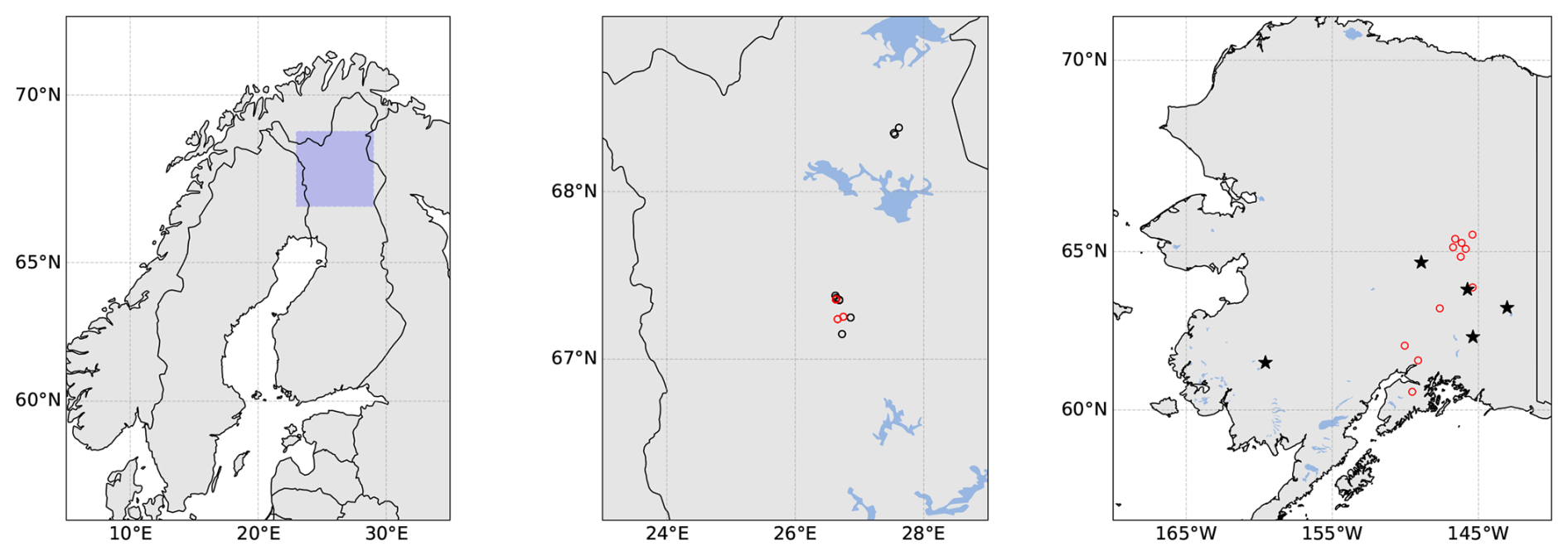
Figure 1 Locations of the chosen training, test, and validation data sites. Left: Northern Finland study area in a broader context (blue squared area). Middle: Location of the chosen model training (black circles) and test (red circles) in situ sites. Right: Location of the chosen model validation in situ sites. Black stars indicate forest sites and red circles indicate other sites (mosaic, shrub, sparse).

2.1 Study area

The main study area is located in Northern Finland, between latitudes 65.5 and 70.0° N, placing it in the boreal forest biome. Based on the land cover classification data in 100 m resolution from CORINE land cover (see Sect. 2.8) for NF (area shown in Fig. 1), around 61 % of the area is covered by tree cover (42 % coniferous trees, 10 % broadleaved trees, and 9 % mixed trees). One fifth of the area (almost 20 %) is covered in peat bogs, and 4.5 % is covered by water bodies (lakes). Water bodies include three large lakes (Lake Inari, Lokka Reservoir, and Porttipahta Reservoir), but also many smaller lakes. The rest of the land use (around 15 %) is different urban areas, heatlands, bare areas, and agriculture.

2.2 SMAP soil moisture

The SMAP mission was meant to combine radiometer (passive) and radar (active) observations. However, since the radar broke down just months after the launch, the radiometer is currently the only instrument observing the surface. This SMAP L-band (1.41 GHz) radiometer has a native spatial footprint of 36 km and the data is provided on the global cylindrical EASE-Grid 2.0 (Brodzik et al., 2012).

SMAP soil moisture is based on retrieved brightness temperature data in horizontal and vertical polarizations (O'Neill et al., 2021). Water body correction is applied to the brightness temperature data first to remove water bodies, as they lower the brightness temperature values and hence cause overestimated soil moisture values. Then tau-omega-model (tau, vegetation optical depth τ and, omega, vegetation single scattering albedo, ω) is applied to the single channel (horizontal and vertical) brightness temperature data to separate soil and vegetation contributions from the total brightness temperature. After that, soil moisture is retrieved by inversion from the tau-omega corrected brightness temperature. Land use classification data is used to determine the τ and ω values for different areas. For dual-channel retrieved soil moisture, the tau-omega corrected single-channel brightness temperature data is used.

In this study, we use the SMAP SPL3SMP V009 product (O'Neill et al., 2023), in which the global surface soil moisture (0–5 cm) in m³ m⁻³ is provided twice a day, at 06:00 am (descending) and at 06:00 pm (ascending). Three different soil moisture products are available, one calculated from each single channel and one dual-channel product. As the latter one is currently the baseline product (Chan and Dunbar, 2021), we chose that for this study. Further, we focus on the soil moisture data at 06:00 am (descending overpasses). This SMAP data in 36 km resolution is used as an input for the soil moisture model.

2.3 MODIS

The Moderate Resolution Imaging Spectroradiometer (MODIS) instruments are aboard the Terra and Aqua satellites, which were launched in 1999 and 2002, respectively. As Sun-synchronous satellites, they provide almost global coverage every 1 to 2 d. Terra is set to a descending orbit (measurements at 10:30 am) and Aqua to an ascending orbit (measurements at 01:30 pm). The MODIS instrument measures multiple wavelength bands, resulting in a wide range of obtained parameters. In this study, we use vegetation indices from both MODIS instruments. We use MYD13Q1 (from Aqua, Didan, 2021a) and MOD13Q1 (from Terra, Didan, 2021b) products (version 6.1) which are global 16-d-mean data sets with 250 m spatial resolution. The data used, the Enhanced Vegetation Index (EVI) and the Normalized Vegetation Index (NDVI), are provided in the Sinusoidal tile grid. EVI and NDVI contribute to the vegetation effects of the soil moisture model.

2.4 SMAP-based 1 km soil moisture data

SMAP, enhanced to 9 km spatial resolution, was further downscaled to 1 km (Lakshmi and Fang, 2023) by using thermal inertia theory (Fang et al., 2022). Based on that theory, the land surface temperature (LST) difference between night and day is negatively correlated to the soil moisture. For downscaling SMAP, the MODIS LST data in 1 km spatial resolution from Terra (night) and Aqua (day) were used, combined with the NDVI, also from MODIS. The NDVI, divided into 10 groups by using an interval of 0.1, is used for grouping soil moisture and LST differences. The assumption behind this is that changes in NDVI affect the relationship between soil moisture and LST difference. Based on the validation, the downscaled SMAP data performs better in low latitudes and warm months, compared to high latitudes and cold months (Fang et al., 2022). The SMAP in 1 km resolution is used in this study as an example of downscaled data based on SMAP data.

2.5 Interpolated daily weather observations

Finnish Meteorological Institute provides different weather-related parameters in spatial resolution of 1 km (Finnish Meteorological Institute, 2023), covering the time period starting from 1961 through the present day. Daily weather station observations are interpolated into a 1 km × 1 km grid by using kriging with external drift. In that method, external predictors are used as covariates. Elevation, relative altitude, the effect of the seas, and the effect of the lakes are the chosen external predictors for these weather station observation based maps (Aalto et al., 2016). Daily precipitation sum and daily mean temperature are used as inputs for the soil moisture model.

2.6 GPM

The Global Precipitation Measurement mission (GPM, https://gpm.nasa.gov/missions/GPM, last access: 23 May 2025) is a network of satellites, aiming to provide precipitation observations every 2–3 h. This is achieved by using active radar observations and passive microwave radiometer measurements. Precipitation data is provided in multiple levels and processing steps, of which we use the level 3 Integrated Multi-satellitE Retrievals for GPM (IMERG) Final Run data. This data is based on intercalibrated data from all microwave precipitation estimates, and microwave-calibrated infrared satellite estimates, as well as bias corrected by using precipitation gauge analyses (Huffman et al., 2023). The Final Run product is provided in either 30-min intervals or daily and monthly means. The spatial resolution is 0.1° (around 10 km). For this study, we use daily means of precipitation.

2.7 ERA5-Land

ERA5-Land, the land component of the fifth generation of European Centre for Medium-Range Weather Forecasts (ECMWF) atmospheric reanalysis of the global climate (ERA5), is produced by the Copernicus Climate Change Service. Similarly to ERA5, the land component also covers the period from 1940 to the present day (Hersbach et al., 2020), but with enhanced spatial resolution (from 31 to 9 km). ERA5-Land provides hourly data of various surface parameters, of which we used air temperature at 2 m above the surface (K).

2.8 CORINE land cover

The Coordination of Information on the Environment (CORINE) program was launched in the 1980s, as there was a need for detailed and harmonized land cover data set over the European continent (Büttner et al., 2017). The current land cover data covers the pan-European area with 100 m spatial resolution. The data set consists of 44 classes, and it is updated every six years. In this study, we use CORINE land cover data from 2018 to determine the land use classifications of the study area, the land cover classes of the used in situ sites in the NF area, and we also used land cover data to create a mask to exclude water bodies and all the other land covers except forested areas.

2.9 In situ data

In situ soil moisture data for model training and testing are from the Arctic Space Centre of the Finnish Meteorological Institute (FMI-ARC, https://fmiarc.fmi.fi/, last access: 23 May 2025). FMI-ARC hosts a measurement infrastructure, which is used to monitor, for example, the atmosphere, soil properties, snow properties, precipitation, and carbon and water cycles. All collected observations can be found at https://litdb.fmi.fi/ (last access: 30 September 2024). For in situ soil moisture observations, the measurement sites are located around Sodankylä and Saariselkä, and they cover mostly boreal forested sites. The chosen in situ sites with additional information can be found in Table A1, and their locations are shown in Fig. 1. The in situ soil moisture is measured at different depths, and for this study, we chose a depth of −5 cm.

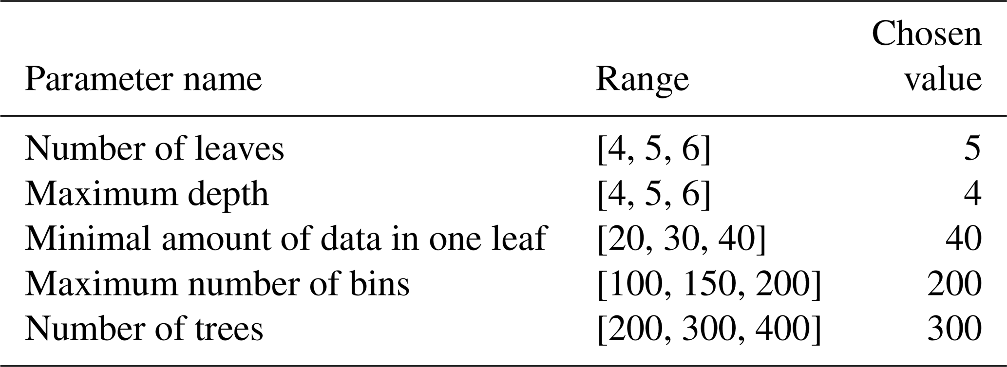
Table 1 Gradient Boosting model parameters, their ranges and chosen values to be used for model building. Parameter ranges are constrained to prevent overfitting. The chosen values are determined by using GridSeachCV method with CV = 3.

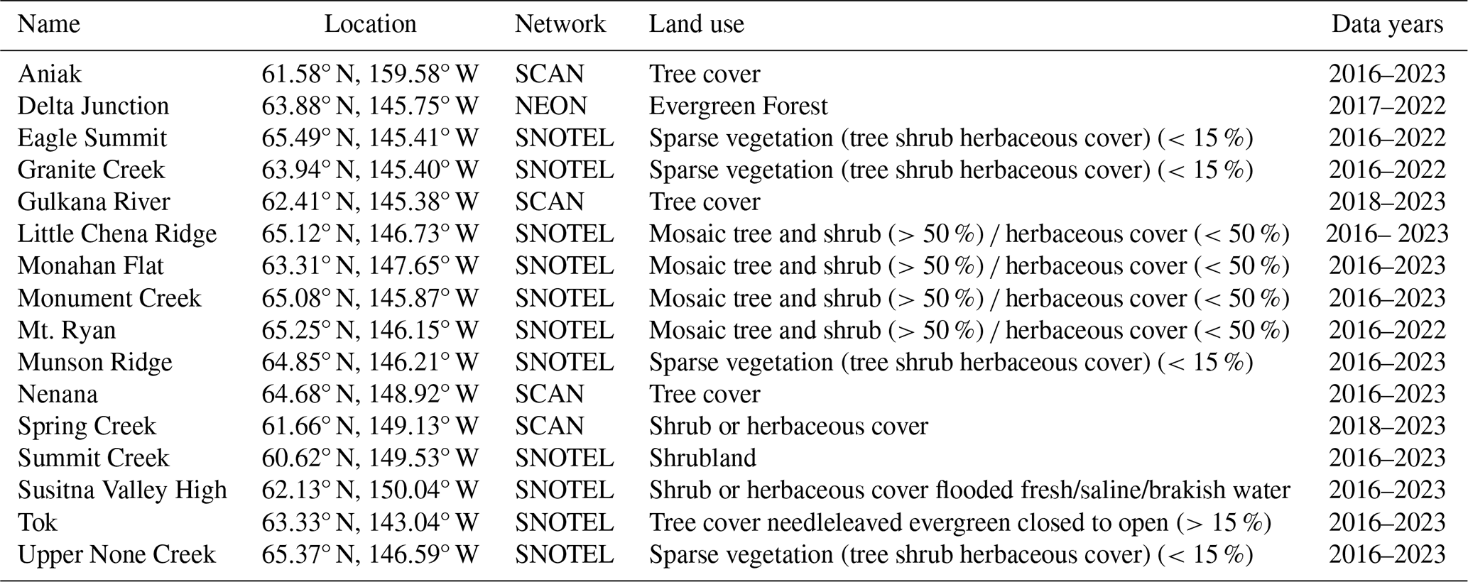
The in situ data for validation of the constructed model are located in the boreal zone in Alaska. In situ soil moisture data has been collected in the International Soil Moisture Network (ISMN) database starting from 1952 (Dorigo et al., 2013, 2021). In situ soil moisture data is provided to the ISMN by multiple organizations for free use. From ISMN we chose 16 stations located in the boreal zone (Fig. 1, right side), and information about those sites can be found in Table A2. Similarly to NF sites, the in situ soil moisture is also measured at different depths, and for this study, we chose a depth of −5 cm.

Additionally, we included one in situ site from the U.S National Science Foundation's National Ecological Observatory Network (NEON). NEON has multiple measurement sites around the United States, of which 5 are located in Alaska. From these 5 sites, we chose Delta Junction as its dominant land use class is evergreen forest. The used data product is DP1.00094.001 (National Ecological Observatory Network, 2025), in which soil volumetric water content is included in various depths. For this study, we chose a depth of −6 cm, which is the shallowest one.

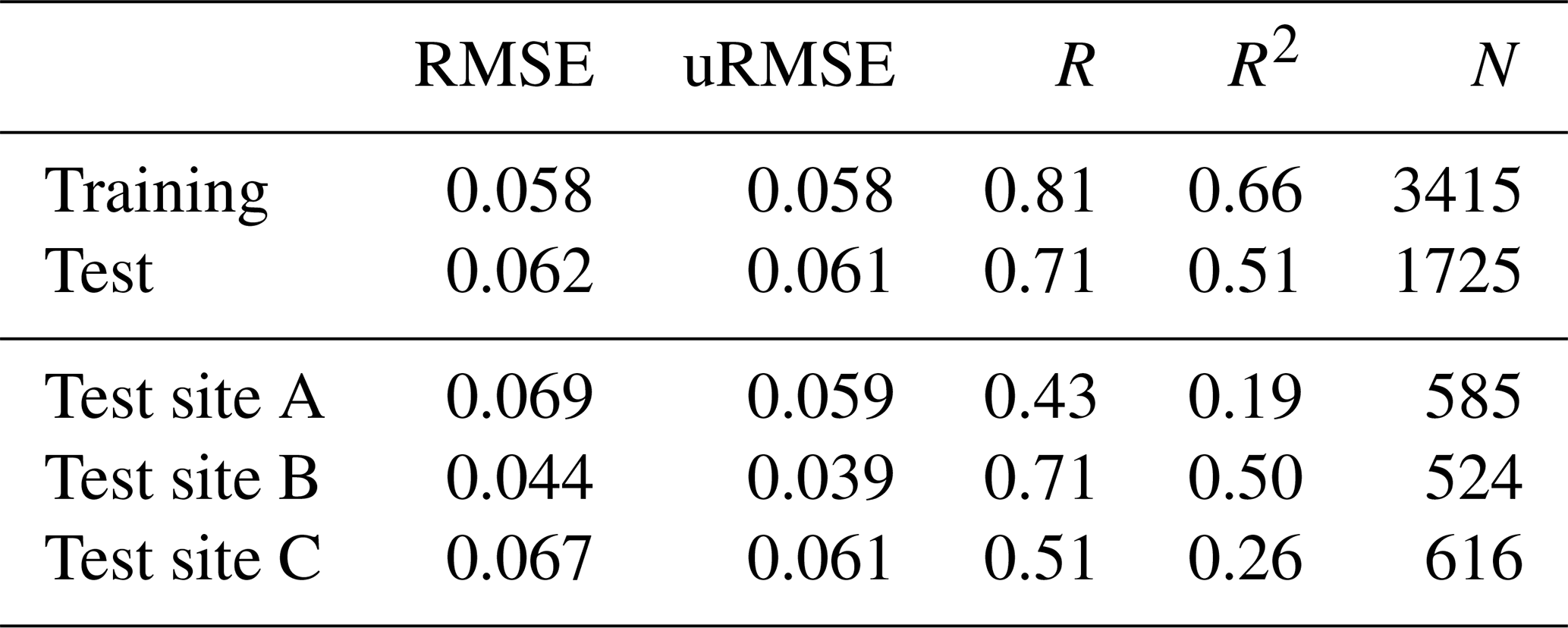
Table 2 Statistical values between predicted values and in situ soil moisture for training and test sets.

3 Methods

3.1 Preprocessing

All gridded data used (SMAP, EVI, NDVI, and interpolated weather station observations) are reprojected to the global EASE2-grid if needed and resampled to achieve a spatial resolution of 1 km. This means that the projection matches that of SMAP, but the spatial resolution is finer than that of SMAP. If the original resolution is coarser than the resampled one, the resampling is done by using the nearest neighbor. On the other hand, if the original resolution is finer than the resampled one, then the resampling is done by taking the average of all values within the coarser pixel. The average is taken even if there is only one value within the coarser pixel. This ensures that the model inputs have a minimal number of missing values.

After resampling and reprojecting, some of the data are further preprocessed. As EVI and NDVI data from both MODIS instruments are originally provided every 16 d, we obtain daily maps of EVI and NDVI by linear interpolation over time using the closest available observations. The linear interpolation was chosen because it is easy to implement and does not cause any major discrepancies in the interpolated data for vegetation types with weak seasonal changes, such as evergreen needle-leaved forests (Li et al., 2021).

After interpolation, we calculate the mean value of Terra and Aqua -based vegetation maps to obtain only one EVI and NDVI map per day. Precipitation and air temperature from interpolated weather station data are provided as daily means. Based on preliminary testing, we decided to use a precipitation sum of 2 and 7 d preceding each SMAP observation, and a temperature sum of 8 and 10 d preceding each SMAP observation instead of using just the daily means of one previous day. This approach takes into account the cumulative effects of temperature and precipitation. In situ data for training and testing was cleaned by removing those stations and those years where soil moisture values were abnormally low (below 0.05 continuously, or decreased to zero regularly), as including those values might lead to the model underestimating soil moisture. Also, there are two in situ sites located in or close to the peatlands, where soil moisture values of those sites are extremely high (>0.75 m³ m⁻³). Including those locations in the training set caused the model to predict erroneous soil moisture values. Therefore, those two sites were excluded from the study data set.

After preprocessing and data cleaning, all the gridded data are matched with NF in situ locations. If there are multiple in situ values within the same 1 km pixel, we take a mean value of those soil moisture values and use that instead to represent the soil moisture in that location. By doing this, we end up with only 10 individual locations, as most of the in situ sites are located near each other.

3.2 Model for soil moisture

The data set for model construction consists of only 10 individual locations. We aimed to have similar distributions of soil moisture values in both training and test sets. Therefore, we chose 7 of those 10 sites for the training data set, and the other 3 were left for the test set. The placing of the individual in situ sites to training or test set is shown in Fig. 1 and Table A1.

We used all the available data from the chosen annual periods covering the years 2019–2023, and hence we had 3415 values for training and 1775 for testing. Tree-based algorithms are commonly used in soil moisture predictions (e.g. Wei et al., 2019; Tramblay and Quintana Seguí, 2022; Ning et al., 2023; Shokati et al., 2024), and it has been reported that tree-based methods can outperform deep-learning methods (Li and Yan, 2024). The Gradient Boosting (GB) method (Breiman, 1997; Friedman, 2001, 2002), in which the weak learners (decision trees) are trained sequentially by correcting the residuals of the previous model, was therefore chosen for model construction. We used a framework for tree-based algorithms called Light Gradient-Boosting Machine (lightGBM), as it is faster to use (Ke et al., 2017).

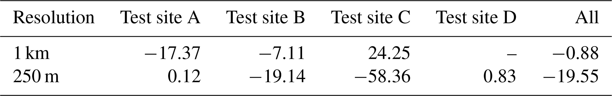
Table 3 Mean relative differences [%] between in situ soil moisture values and predicted soil moisture estimates from both GB model. Values are from test set, and they cover the time period 2019–2023.

We hypertuned the model parameters by using the GridSearchCV method from scikit-learn (Pedregosa et al., 2011). It is a method where all possible combinations of given model parameters and their grids are tested and evaluated by using cross-validation. In our model building, we used CV = 3. The chosen parameters with their test ranges are shown in Table 1. The learning rate was chosen to be 0.05. We also limited the maximum bins to 200, and a minimum number of data values in one leaf to 40 at maximum to limit overfitting.

4 Results

4.1 Analysis of the model

The SHapley Additive exPlanations (SHAP, Lundberg et al., 2020) values (which specify the effect of different individual inputs on the output) indicate that vegetation inputs dominate the results, as can be seen from Fig. 2. All inputs have clear linear effects on the results. Precipitation-related inputs have the smallest effect on the model.

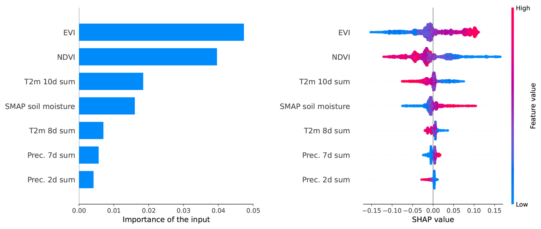
Figure 2 The SHapley Additive exPlanations (SHAP) values for the constructed gradient boosting model. Left: the mean SHAP values for each predictor. Right: More detailed view of the effect of different feature values on predictions.

The RMSE, R, and R² values between the training and test set indicate no overfitting (Table 2). RMSE and uRMSE values between in situ values and training and test sets are almost identical (0.058 and 0.062, and 0.058 and 0.061, respectively). On the other hand, R and R² values are higher between in situ values and predicted soil moisture values from the training set compared to values between in situ values and test set predicted soil moisture values. Based on results in Fig. 3, there is a possibility of the model underestimating higher soil moisture values (>0.3 m³ m⁻³). Also, as there are no higher than 0.4 m³ m⁻³ soil moisture values in the training set, the model will have difficulties predicting soil moisture values above 0.4 m³ m⁻³.

As the original highest spatial resolution of some inputs is 250 m (NDVI and EVI), we also resampled SMAP soil moisture and weather-related inputs to that same 250 m spatial resolution using nearest neighbor resampling. We then calculated soil moisture maps from those 250 m resolution data maps using the constructed GB model to study how sensitive the developed model is to small changes in vegetation values (i.e. as those are the only parameter values changing within one time step). Exemplary time series for NF test sites for the year 2020 are shown in Fig. 4. The individual in situ sites are located close to each other and therefore the Test sites A–B have the same in situ sites in both resolutions. Only in Test site C one site (MET0010) locates in a different pixel. Therefore, for Fig. 4, we have added an extra Test site D, which includes the in situ site MET0010. Overall, as all sites (A–D) are boreal forest sites, SMAP soil moisture is temporally well in line with in situ soil moisture values, but due to the coarse resolution, there are systematic differences, especially in Test site C (and D). Predicted values calculated for both 1 km and 250 m resolution data are better in line with in situ values. Based on these results for NF sites, the developed model is not overly sensitive to small changes in weather-related and vegetation properties data. Also, based on these time series results, the developed model detects temporal changes well. In hindsight, as the model is constructed using SMAP soil moisture, and SMAP soil moisture data is noisy, some of the same noisy features can be found in predicted values. Also, due to the SMAP being the basis for the developed model, the predicted values have the same temporal resolution as SMAP, meaning that data can be predicted almost daily if SMAP soil moisture data are available. Mean relative differences (Table 3) between in situ values and GB model-based predicted values indicate varying under- and overestimations. In 1 km resolution, the underestimation for the whole test set is just <1 %, which is to be expected. For 250 m resolution, the underestimation is higher, almost 20 % for the whole test set.

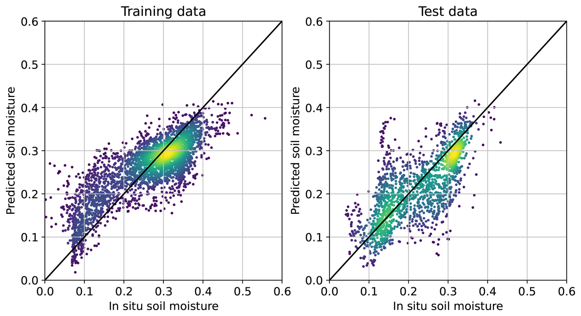
Figure 3 Scatter plots of predicted training and test set soil moisture values from years 2019–2023. Left: scatter plot of training data set. Right: scatter plot of test set.

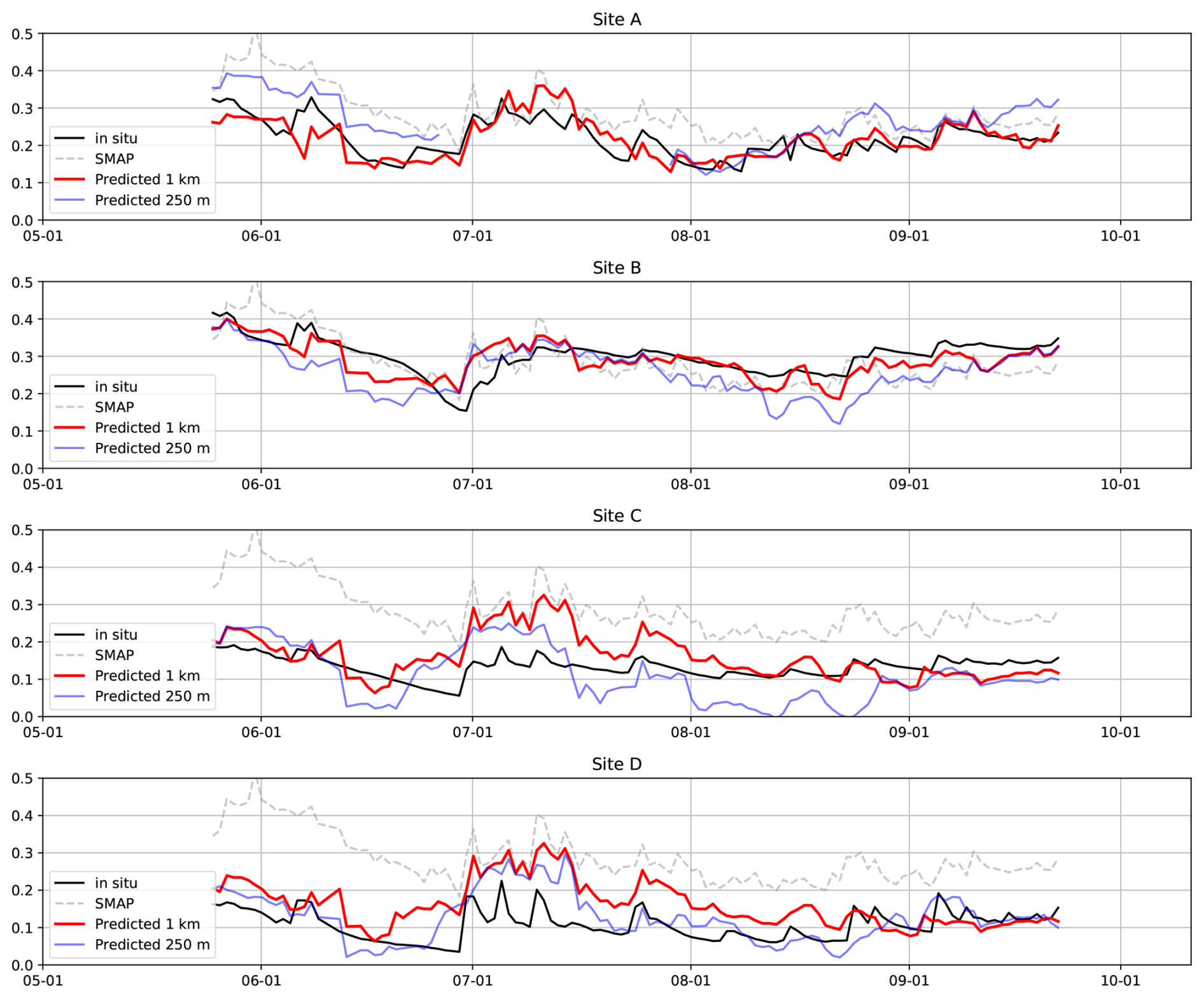
Figure 4 Exemplary time series of test sites for the year 2020. Predicted soil moisture values in 1 km and 250 m resolutions are from a developed gradient boosting model. In test site C, one in situ site (MET0010) locates in different pixel in 250 m resolution. Therefore, we added an extra Test site D, which includes the in situ site MET0010.

We also calculated the soil moisture values for the whole NF area using the constructed model to analyze how well the model captures the spatial variations and also to show the impact of missing pixels on the predicted maps. We calculated soil moisture maps using 1 km and 250 m resolution data. Examples of these predicted soil moisture maps are shown in Figs. 5 and 6. Predicted soil moisture values are lower than SMAP soil moisture values, and for 250 m resolution maps the number of missing pixels increases. Nevertheless, spatial changes are well detected by the predicted values when compared to SMAP soil moisture. The missing values in predicted maps are due to the missing data in the inputs. SMAP data have missing data because of water bodies or otherwise failed soil moisture retrievals. Similarly, vegetation properties are not retrieved over water bodies, but vegetation data are also missing because of missing measurements, caused typically by cloud cover (as vegetation properties are based on optical data). Furthermore, as the model is developed mainly for forested areas, a land cover mask was applied to the results (shown only in Fig. 6, and omitted in Fig. 5 for clarity). We used CORINE land cover data in 100 m spatial resolution as the basis of the mask. Land cover data was resampled to the 1 km and 250 m spatial resolutions and those pixels where forest classes covered under 50 % of the coarser pixel were masked.

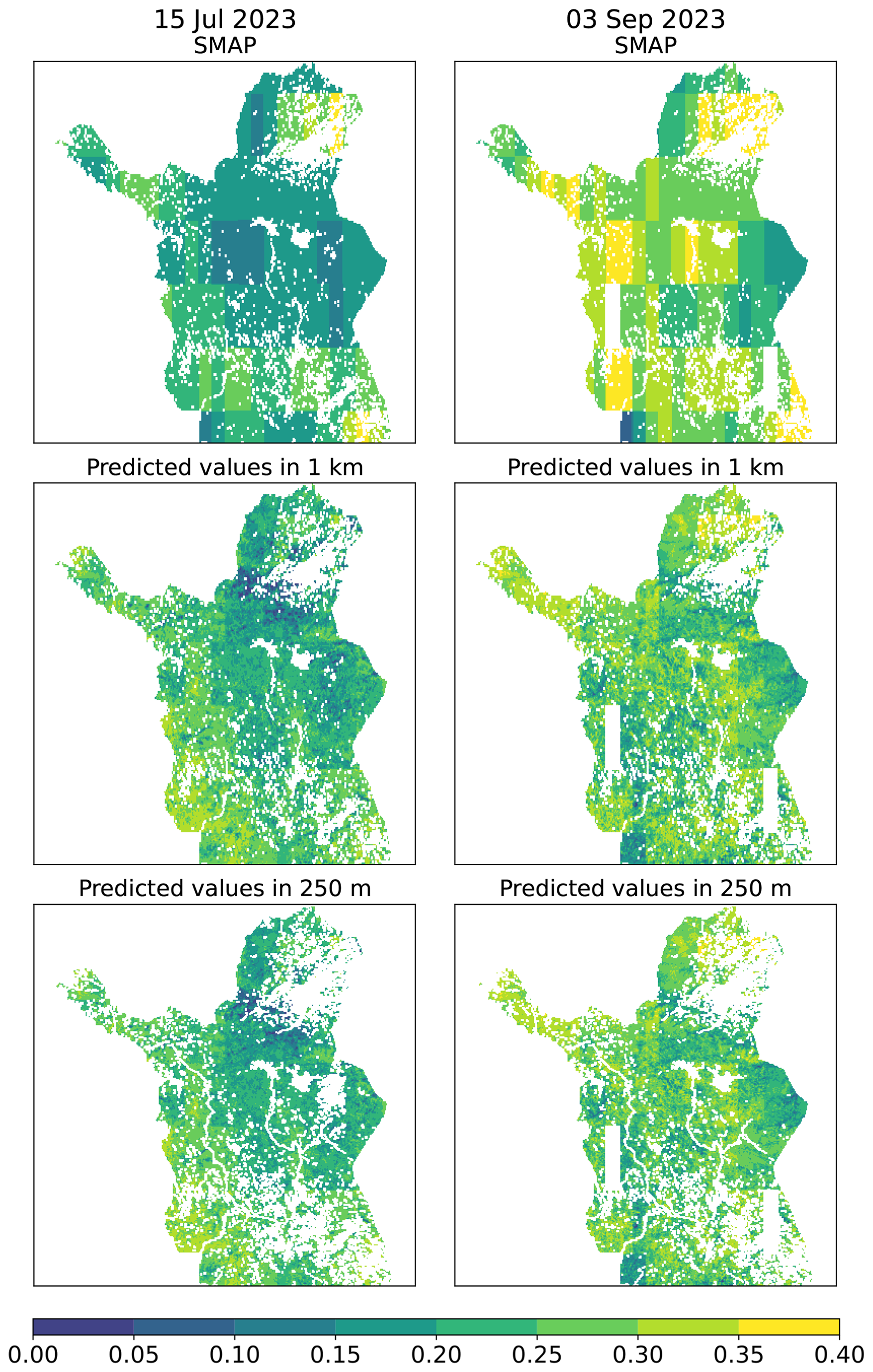
Figure 5 Exemplary maps show SMAP soil moisture for two dates, along with predicted soil moisture at spatial resolutions of 1 km and 250 m. Missing values due to the missing values in inputs and water bodies are indicated in white. Even though developed model is just for forested areas, all pixels with data in these maps are shown for clarity.

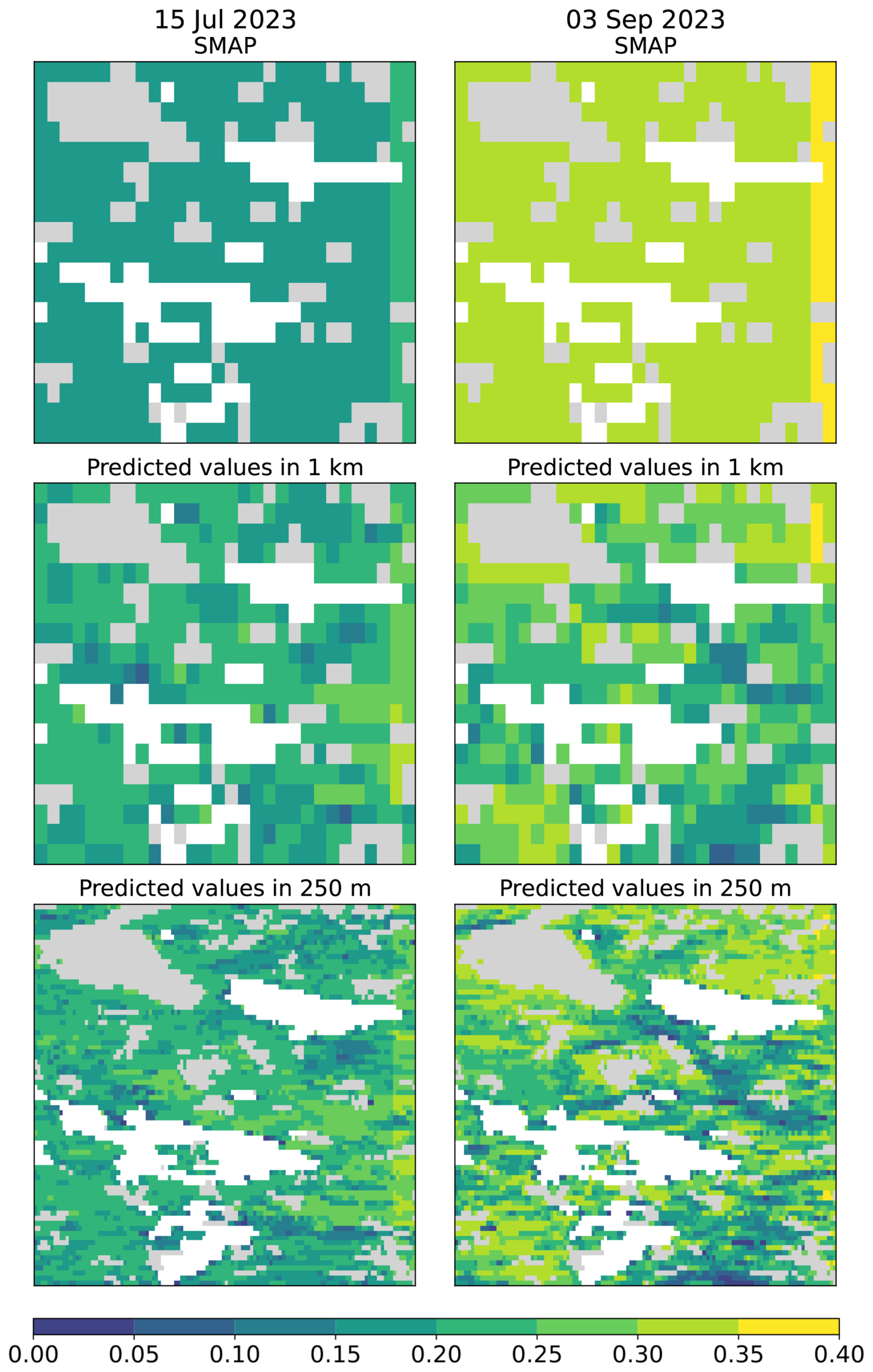
Figure 6 Exemplary maps show SMAP soil moisture for two dates, along with predicted soil moisture at spatial resolutions of 1 km and 250 for a smaller area located around Lake Pallas (68.033° N, 24.197° E). Missing values due to the water bodies are indicated in white and other land uses than forest are indicated in grey. The land use mask is based on CORINE land use classification in 100 m resolution. Pixel is assumed to be forest if the forest class fraction is above 50 %.

4.2 Model uncertainty

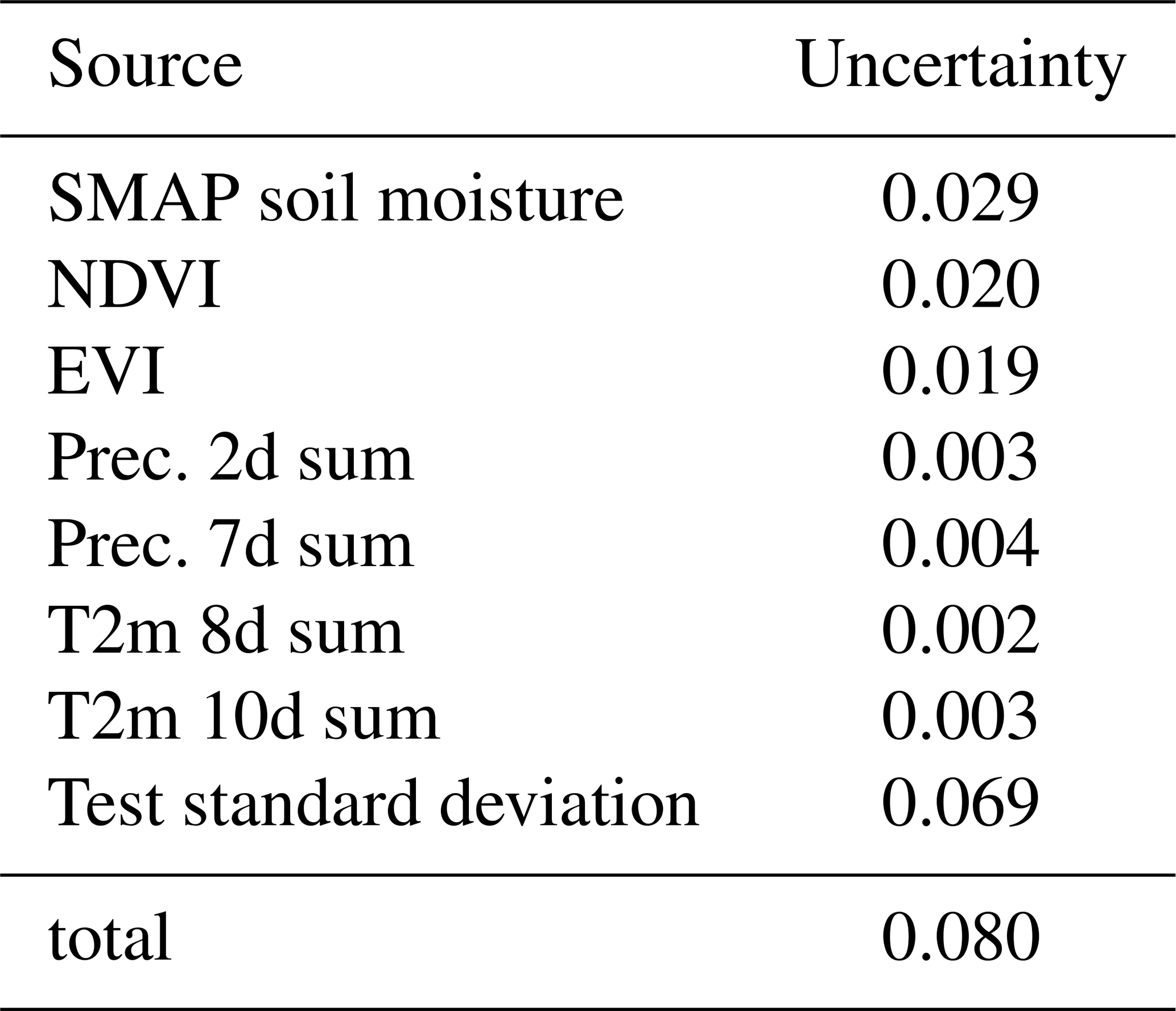
We used the sensitivity of the most important inputs and the standard deviation of the difference between predicted soil moisture values and in situ values from test data as the uncertainty of the model. First, we approximated the uncertainty each input causes to the results. Predicted soil moisture from the training data was used as the reference data. Then we added errors to the important inputs separately from their error distributions $\mathit{ϵ}\sim \mathcal{N}(\mathrm{0},{\mathit{\sigma }}^{\mathrm{2}})$. For vegetation indexes, we used the reported uncertainties, 0.015 for EVI and 0.025 for NDVI (https://modis-land.gsfc.nasa.gov/ValStatus.php?ProductID=MOD13, last access: 15 May 2025). For SMAP soil moisture, we used the standard deviation from the difference between SMAP soil moisture and in situ soil moisture from the whole in situ data set from NF. The obtained standard deviation was 0.097. For weather-related inputs, we used reported RMSE values (Aalto et al., 2016), 1.4 mm for precipitation and 0.58 °C for temperature. As we use cumulative sums, we used error propagation of sum to estimate the uncertainty of them. The uncertainties have therefore a form of $\sqrt{x}\cdot {\mathrm{RMSE}}_i$, where x in the number of days the cumulative sum is obtained, and i is either precipitation or temperature. This way we obtained 1.98 mm uncertainty for precipitation sum over 2 d, and 3.7 mm uncertainty for precipitation sum over 7 d, and 1.64 and 1.83 °C uncertainties for temperature sums over 8 and 10 d, respectively. We calculated the difference between the error-added values and the reference data 100 times. The sensitivity of each varied input, the test std, and the total uncertainty for the constructed model are shown in Table 4. The total uncertainty is calculated as a squared sum between the individual sensitives and test std, that is:

$$\begin{array}{}\text{(1)}& \mathit{ϵ}=\sum _i^N\left(u_i^{\mathrm{2}}\right).\end{array}$$

SMAP soil moisture has the highest impact on the model uncertainty for individual inputs. On the other hand, vegetation properties and weather-related data have the lowest impact. In total, the model uncertainty is around 0.080 m³ m⁻³.

Table 4 Sensitivities for chosen inputs, standard deviation between test set in situ soil moisture and predicted soil moisture, and calculated total uncertainty of the model. All results have the unit m³ m⁻³.

4.3 Validation with Alaska sites

The weather station network over Alaska is sparse, and thus kriging-based interpolation to obtain precipitation and temperature in high resolution (as done over Northern Finland) is not possible. Therefore, we decided to use satellite-based data for precipitation (GPM data) and for temperature, we used ERA5-Land temperature data. GPM data was calculated to required cumulative sums without any modifications, but as ERA5-Land data is provided hourly, we preprocessed it in daily mean temperatures and then further processed it to required cumulative sums.

Altogether 17 stations from Alaska were used as an independent model validation set. One site located in Alaska, Tokositna Valley, was excluded from the validation set, because its soil moisture values varied abnormally. In addition, the predicted soil moisture values below 0.05 m³ m⁻³ were also excluded. We calculated statistical values (RMSE, uRMSE, and R) for each site between in situ soil moisture and SMAP in 36 km resolution, SMAP enhanced to 1 km resolution, and GB-model-based predicted values, both 1 km and 250 m. The median statistical values are similar (Fig. 7), only R values are slightly higher with SMAP in 36 km resolution compared to others.

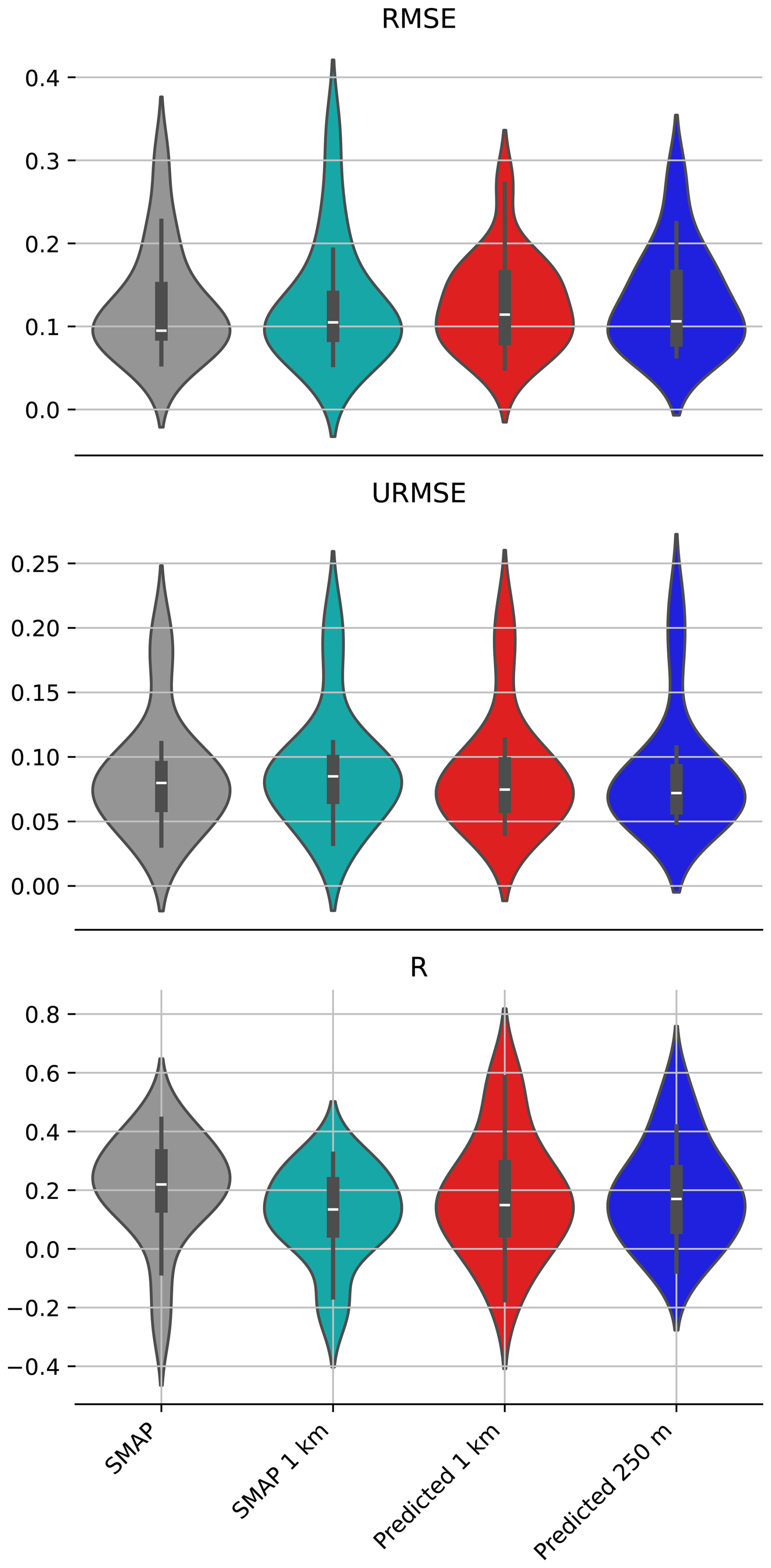
Figure 7 RMSE, uRMSE, and R values between in situ values from Alaska validation data set and different soil moisture data sets (SMAP in 36 km resolution, SMAP in 1 km resolution, predicted values using 1 km resolution data, and 250 m resolution data) shown as violin plots. The data is from the annual time period between 1 May and 15 October, covering varying number of years depending on the in situ site.

Of the 16 stations, only 5 were reported to be located in forested sites (information is based on ESA CCI Land Cover (ESA, 2017) and NLCD (https://www.mrlc.gov/, last access: 12 May 2025)). Soil moisture data comparisons from those five sites are shown in Fig. 8. SMAP soil moisture in both resolutions has a lot of variability compared to predicted estimates. It is also evident that the GB-model cannot predict high soil moisture values (>0.4 m³ m⁻³), as was expected. Overall, there are clear correlations between satellite-based estimates and in situ soil moisture values when taking into account all data, but correlations are less clear when focusing on individual sites.

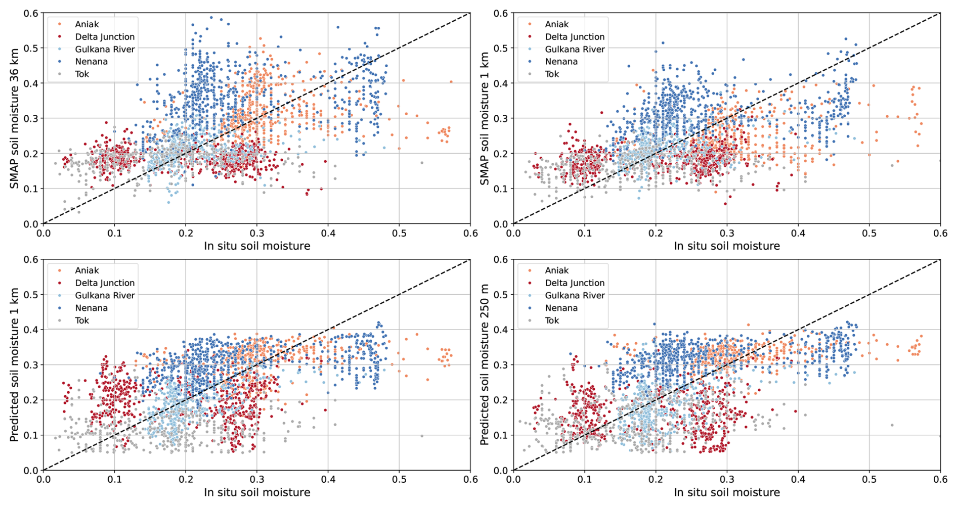
Figure 8 Comparisons between in situ values from Alaska sites (five forested sites) and different soil moisture data sets (SMAP in 36 km resolution, SMAP in 1 km resolution, predicted values using 1 km resolution data, and 250 m resolution data). The data is from the annual time period between 1 May and 15 October, covering varying number of years depending on the in situ site.

Exemplary time series for sites Nenana and Gulkana River (tree-covered sites) are shown in Fig. 9, and a close-up focusing on the year 2019 in Fig. 10. The high soil moisture values at the beginning of the summer (due to the snow melt) are not detected by SMAP data. On the other hand, the GB-model-based estimates do catch them better. Otherwise, SMAP data in both resolutions detect the soil moisture values well. The GB-model-based soil moisture estimates have more temporal variation compared to SMAP data. The close-up of the year 2019 shows that the model can detect the U-shape of the in situ soil moisture better than SMAP data.

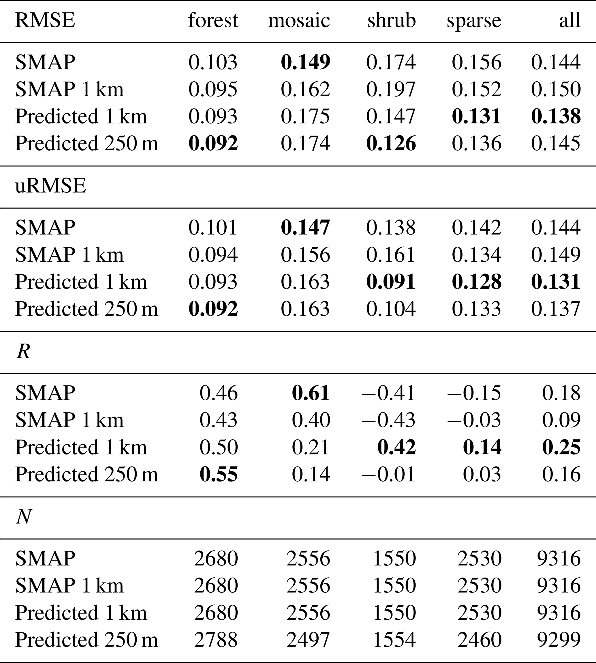
Sixteen in situ sites in Alaska were grouped into coarser land use classification classes (forest, mosaic, shrub, and sparse), and RMSE, uRMSE, and R values were calculated between in situ values and each satellite-based data, the values are shown in Table 5. For forested sites, predicted values in 250 m have the lowest RMSE and uRMSE, and highest R values compared to other data sets. Predicted values in 1 km resolution have the second-highest model validation statistics. For mosaic sites, SMAP in 36 km has the lowest RMSE and uRMSE, and the highest R value. All data sets struggle to predict soil moisture values in sparse sites. In shrub sites, predicted values in 1 km resolution are more in line with in situ values compared to SMAP soil moisture values in both resolutions. Based on these validation results, the developed model predicts temporal changes relatively well.

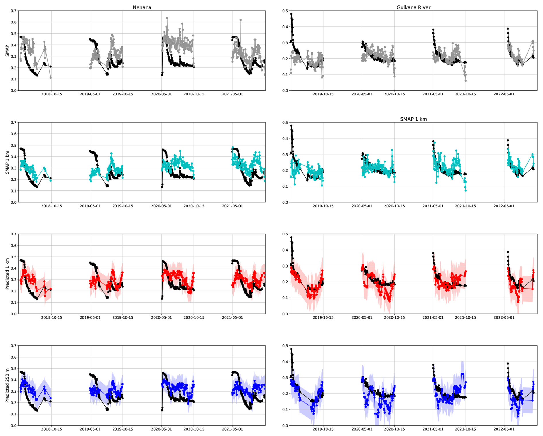
Figure 9 Exemplary time series of soil moisture for two Alaska sites located in forested areas. Left: Nenana, right: Gulkana River. Black indicates in situ soil moisture and grey, turquoise, red, and blue satellite-based soil moisture data. The curtain in the two bottom rows indicates the model uncertainty (uncertainty 0.080 m³ m⁻³ added and subtracted from the predicted values). Data for Nenana is from years 2018–2021, and for Gulkana River from years 2019–2022.

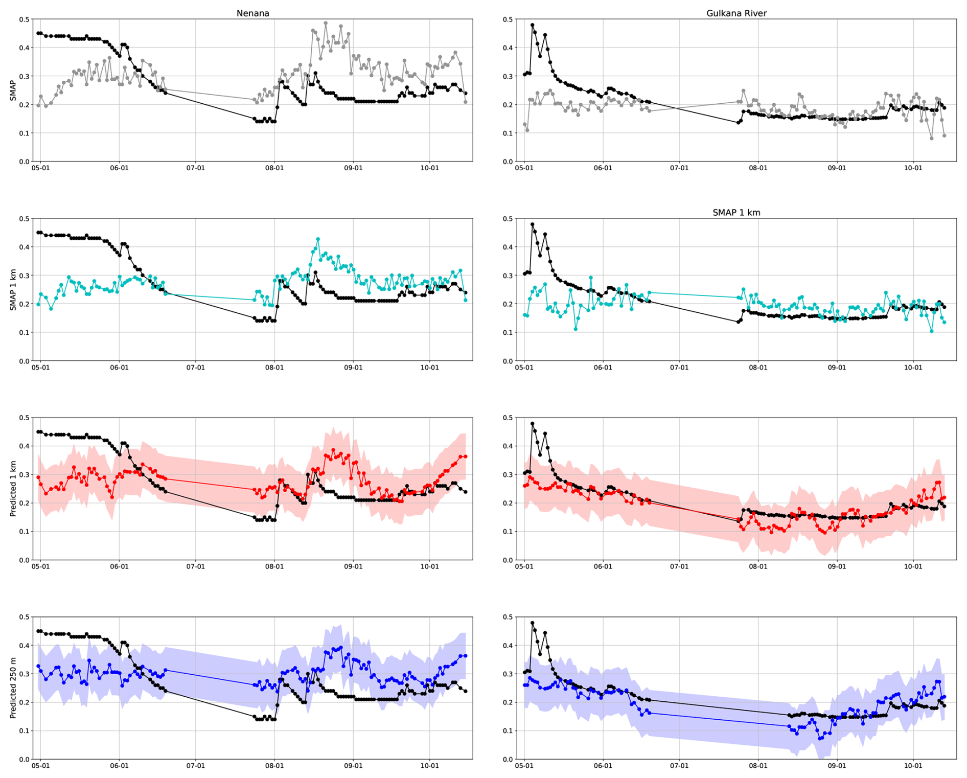
Figure 10 Close-up from the exemplary time series for two Alaska sites located in forested areas. Left: Nenana right: Gulkana River. Black indicates in situ soil moisture and grey, turquoise, red, and blue satellite-based soil moisture data. The curtain in the two bottom rows indicates the model uncertainty (uncertainty 0.080 m³ m⁻³ added and subtracted from the predicted values). Data are from the year 2019.

Table 5 Model validation statistics between observed in situ soil moisture from Alaska sites and predicted soil moisture values. Highlighted values in bold indicate the lowest RMSE and uRMSE values, and the highest correlation values.

5 Discussion

Spatio-temporal data on the variation in soil moisture for boreal regions is crucial for predicting forest-related phenomena, such as tree growth and forest fire risk, both of which influence the carbon storage capacity of these ecosystems. However, existing satellite-based soil moisture products for vegetated areas often have coarse spatial resolution. To address this issue, higher-resolution data is necessary to capture the finer spatial variations in soil moisture. Consequently, we developed a model utilizing satellite data to estimate soil moisture at high resolution (1 km and 250 m) over boreal forested regions. We used a tree-based machine learning method called gradient boosting with SMAP soil moisture in 36 km spatial resolution as a basis. Produced data maps have the same temporal resolution as SMAP (typically daily, but are missing if SMAP soil moisture retrieval has failed). The developed model is shown to retain the temporal and spatial variability of SMAP soil moisture, but validated against independent data, the predicted values show better agreement compared to the SMAP soil moisture (RMSE decreasing from 0.103 to 0.092 m³ m⁻³, and correlation increasing from 0.46 to 0.55 over forest sites).

There exist numerous other soil moisture products at a 1 km spatial resolution, which differ on the underlaying data they use, the methods they implement, and also whether they are global or regional (Table 6). Overall, our constructed model has higher uRMSE values than many other 1 km spatial resolution data sets, but most of them do not cover boreal forest areas or are not validated against boreal forest soil moisture. Of those that do cover boreal forests, the uRMSE and R² values are in line with the results we obtained from validation against forested sites in Alaska. Those data products which are based on Sentinel-1 SAR and cover boreal forest zone (Bauer-Marschallinger et al., 2018; Fan et al., 2025; Meyer et al., 2022) have difficulties with dense vegetation, which is to be expected due to the C-band being sensitive to vegetation. On the other hand, good results are obtained when using ERA5 soil moisture as the basis data (Zhang et al., 2023). Used downscaling methods and algorithms vary. Change detection method (used in Bauer-Marschallinger et al., 2018) and forward model (Fan et al., 2025) are used for Sentinel-1 SAR data, whereas for Sentinel-1 and SMAP combination uses SMAP active-passive algorithm (used in Das et al., 2019; Meyer et al., 2022, and is based on work by Das et al., 2014, 2018; Entekhabi et al., 2014). Machine-learning methods are also implemented (Kovačević et al., 2020; Rao et al., 2022; Zhang et al., 2023, 2024; Zheng et al., 2023), mostly when using ESA-CCI or ERA5 soil moisture data. When SMAP soil moisture is used as a data source, typical algorithms are based either on the thermal inertia theory (used in Fang et al., 2022; Dandridge et al., 2020) or the Temperature–Vegetation (T–V) method (used in Yin et al., 2020; Mohseni et al., 2024, based on Sandholt et al., 2002). Once again, the validation results from our constructed ML-method-based model are consistent with other ML-based data sets.

Bauer-Marschallinger et al. (2018)Fan et al. (2025)Das et al. (2019)Meyer et al. (2022)Kovačević et al. (2020)Zhang et al. (2024)Zheng et al. (2023)Zhang et al. (2023)Fang et al. (2022)Yin et al. (2020)Dandridge et al. (2020)Mohseni et al. (2024)Rao et al. (2022)

Table 6 A collection of downscaled soil moisture data sets in 1 km spatial resolution, with reported accuracies. The uRMSE values have the unit m³ m⁻³.

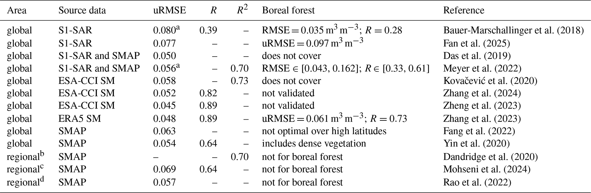
^a RMSE instead of uRMSE. ^b Lower Mekong River Basin. ^c Africa. ^d China.

Soil properties are commonly used inputs for soil moisture models (e.g. Ranney et al., 2015; O et al., 2022; Ma et al., 2023; Zhang et al., 2023). As we have a small number of individual sites in training and test sets, we excluded soil properties data from this study. Additionally, other commonly used inputs include topography and geography data (i.e. elevation, slope, aspect, latitude, and longitude). Again, as we have a relatively small amount of model construction data, adding geographical information would have caused major overfitting. We also excluded topography data, as it has been found that models using topography data as inputs may not be useful in other locations (Kemppinen et al., 2023). Weather-related data, i.e. precipitation, and temperature, are included as inputs because they are related to the soil moisture. Precipitation is positively correlated with soil moisture (Sehler et al., 2019), but air temperature has the opposite effect (Feng and Liu, 2015). Based on feature importances (Fig. 2), air temperature in both cumulative sums (sums over 8 and 10 d) have a negative impact on the results as expected, but precipitation has a varying effect. Precipitation sum over 7 d has the expected positive effect, but the precipitation sum over 2 d has the opposite effect. The latter might be due to the canopy interception and no-rain values. The canopy interception of precipitation can be up to 50 % in the dense boreal forest (Molina and del Campo, 2012; Zabret et al., 2017; Hassan et al., 2017), leading to only a small amount of rain attributed to the soil moisture, but also it is possible that there are no rain events happening, leading the sum of rain over 2 d to cause negative effect to the soil moisture values. It has also been studied that air temperature has a higher impact on soil moisture than precipitation, even over forest areas (Feng and Liu, 2015). This effect can be seen in feature importances (Fig. 2), as temperature has a clearly higher impact on the soil moisture estimates compared to precipitation. The cumulated precipitation and temperature values increased the model accuracy compared to the instantaneous values, and therefore they were chosen. An additional useful data source would have been the land surface temperature (LST), as the LST difference between night and day correlates with soil moisture. LST data has been widely used for estimating soil moisture (e.g. Matsushima et al., 2012; Hao et al., 2022; Han et al., 2023). The disadvantage of LST is that it is obtained from optical measurements. Due to the difficulties caused by cloud cover, obtaining even moderately gap-free LST data regularly over the whole NF area was an impossible task, and therefore we did not include LST as an input.

To choose the best model, we tested three tree-based methods: random forest, level-wise gradient boosting, and leaf-wise growth-based gradient boosting. The leaf-wise growth GB (lightGBM) produced the results with the highest accuracy and was therefore chosen. However, because it is a tree-based method, it cannot extrapolate well when inputs differ from training data, as the decision boundaries are determined during training. Therefore, our predicted estimates are more or less bounded, and unexpectedly high or low soil moisture values are not predicted correctly (i.e. soil moisture values below 0.05 m³ m⁻³ or above 0.4 m³ m⁻³). To overcome this disadvantage, there needs to be much more data from diverse in situ locations. The available data from the in situ networks is limited and thus hinders model’s predictive ability.

We included SMAP in 1 km resolution to be compared to our model predictions. Other downscaled data sets were also considered, but as the soil moisture network is sparse, they, unfortunately, use some of the same in situ sites from NF and Alaska for training, and therefore we could not use them as independent data sets. The comparisons with SMAP in 1 km resolution indicate that downscaled SMAP lacks some of the variability found in our model. For some sites in Alaska, SMAP in 1 km even performed weaker compared to SMAP in 36 km resolution. Based on those results, it could be possible that thermal inertia theory is not ideal for downscaling soil moisture data over forested areas.

As our model provides high-resolution soil moisture for forested areas, it covers approximately 60 % of the NF area (see Sect. 2.1). Additionally, SMAP soil moisture has a lot of noise, and some of those features are also transferred to our model predictions. Smoothing would have been one option to decrease the effect of noise, but choosing the method that would have retained the actual temporal variations was not a straightforward task. Also, we tried to implement precipitation and temperature data to smooth some of the noise, but due to the dense nature of the boreal forest, there was no clear relationship between soil moisture changes and weather. Therefore, we decided to leave the noise in the end results.

In the future, L-band-based missions, like the NASA-ISRO SAR mission (NISAR, https://nisar.jpl.nasa.gov/, last access: 23 May 2025; Lal et al., 2023, 2024) with a planned launch around April 2025, and Radar Observing System for Europe in L-band (ROSE-L, https://sentiwiki.copernicus.eu/web/rose-l, last access: 23 May 2025) with a planned launch in 2028, are aiming to provide soil moisture data with higher spatial resolution (around 200 m for NISAR and around 25 m for ROSE-L). With those resolutions, even peatlands can be taken into account. As they cover over 20 % of NF and are important carbon sinks, peatlands need to be included in soil moisture studies. If there were more in situ observation sites located in varying kinds of peatlands, one could construct a model based on them, and then combine models focused on forested areas and peatlands to better account for all the variability in soil moisture over boreal forest areas. As it is, the constructed GB-model does provide an alternative to downscale SMAP soil moisture in 36 km resolution to finer spatial scales over boreal forests.

6 Conclusions

We developed a model to predict high-resolution soil moisture in boreal forests. This model specifically targets forests, as peatlands are not represented in SMAP soil moisture data, and most in situ soil moisture observation sites are located within forests. The model was developed by using SMAP soil moisture at 36 km spatial resolution as the basis data, and additional vegetation properties and weather-related data were used to guide the machine learning model together with in situ soil moisture values. The model produces predictions at a resolution of 1 km, which aligns well with SMAP measurements. However, it can also generate soil moisture estimates at a finer resolution of 250 m, offering improved accuracy in certain applications, for example hydrological modelling and carbon exchange studies. Consequently, the model provides a valuable tool for predicting soil moisture in high resolution across boreal forested landscapes.

Appendix A

Table A1 In situ sites for training and testing the soil moisture model, located in Northern Finland. Land cover information is from CORINE land cover data set.

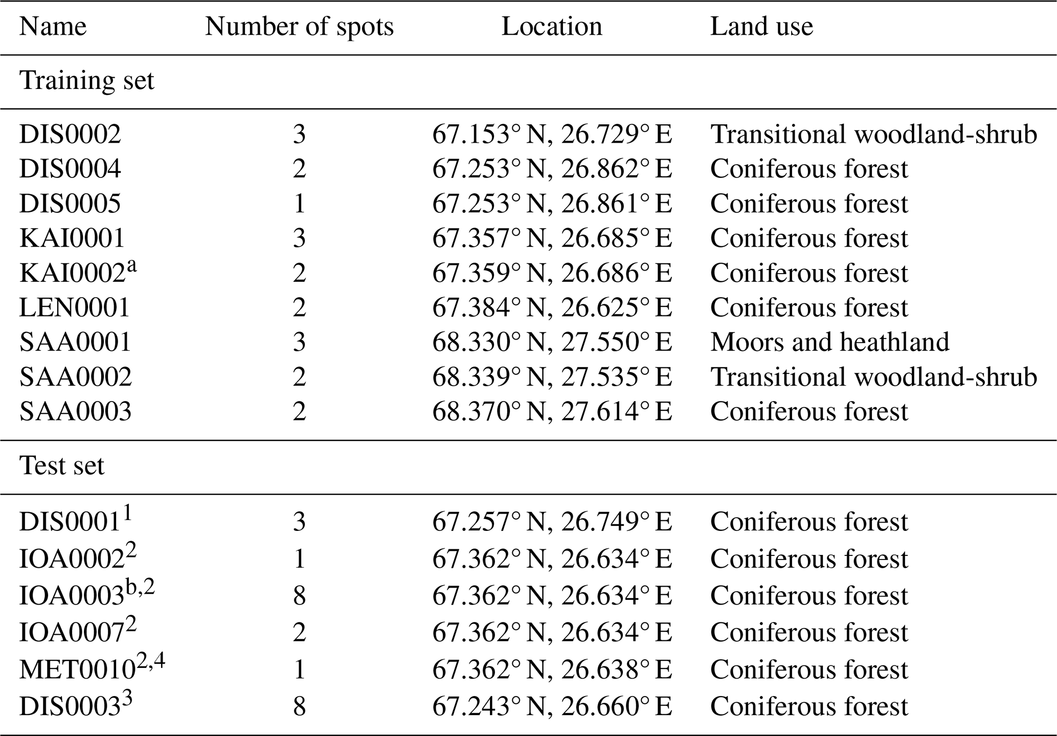
^a KAI0002 has 3 spots, but one of them had abnormally low soil moisture values and was therefore removed. ^b IOA0003 has 8 spots, but two of them had abnormally low soil moisture values and were therefore removed. ¹ Test site A. ² Test site B. ³ Test site C. ⁴ Test site D in 250 m resolution.

Table A2 In situ sites for model validation, sites located in Alaska. Data are from four different networks, SCAN (Schaefer et al., 2007), SNOTEL (Leavesley et al., 2008), USCRN (Bell et al., 2013), and NEON (National Ecological Observatory Network, 2025). Land cover information for SCAN, SNOTEL, and USRN sites is from ESA CCI Land Cover (ESA, 2017), and for NEON, the land cover information is from NLCD (https://www.mrlc.gov/, last access: 23 May 2025).