Integrating historical archives and geospatial data to revise flood estimation equations for Philippine rivers

Flood magnitude and frequency estimation are essential for the design of structural and nature-based flood risk management interventions and water resources planning. However, the global geography of hydrological observations is uneven, with many regions, especially in the Global South, having spatially and temporally sparse data that limit the choice of statistical methods for flood estimation. To address this data scarcity, we pool all available annual maximum flood data for the Philippines to estimate flood magnitudes at the national scale. Available river discharge data were collected from publications covering 842 sites, with data spanning from 1908 to 2018. Of these, 466 sites met criteria for reliable estimation of the annual maximum flood. Using the index flood approach, a range of controls was assessed at both national and regional scales using modern land cover and rainfall data sets, as well as geospatial catchment characteristics. Predictive equations for 2 to 100 year recurrence interval floods using only catchment area as a predictor have R²≤0.59. Adding a rainfall variable, the median annual maximum 1 d rainfall, increases R² to between 0.56 for Q₁₀₀ and 0.66 for Q₂. Very few other topographic or land use variables were significant when added to multiple regression equations. Relatively low R² values in flood predictions are typical of studies from tropical regions. Although the Philippines exhibits regional climate variability, residuals from national predictive equations show limited spatial structure, and region-specific equations do not significantly outperform the national equations. The predictive equations are suitable for use as design equations in ungauged catchments for the Philippines, but statistical uncertainties must be reported. Our approach demonstrates how combining individually short historical records, after careful screening and exclusion of unreliable data, can generate large data sets that can produce consistent results. Extension of continuous flood records by continuous and rated monitoring is required to reduce uncertainties. However, the national-scale consistency in our results suggests that extrapolation from a small number of carefully selected catchments could provide nationally reliable predictive equations with reduced uncertainties.

1 Introduction and rationale

The impact of river flooding across Southeast Asia is severe on a global scale, whether measured in terms of the inundated area, the number of people affected, or fatalities (Ziegler et al., 2020). Understanding the hazard and designing mitigation or adaptation strategies rely on estimating flood magnitude and frequency, which is achieved through empirical analyses of available data and, for forecasting, the results of climate and hydrological models. The resulting equations to estimate flows of specified recurrence are used for a wide range of purposes, including insurance loss estimation (Lyubchich et al., 2019), aquatic biodiversity assessment (Parasiewicz et al., 2019), engineering design, and water resource planning.

Estimating flood magnitude and frequency is crucial for designing mitigation strategies, and estimates are typically made using empirical analyses that generate predictive models. A wide range of statistical methods have been applied to flood frequency estimation (see Asquith et al., 2017 for a recent listing). The index flood approach uses the median or mean annual maximum flood, or equivalently a flood of specified recurrence interval, and relates this to catchment properties to develop regional predictive equations (e.g. Dalrymple, 1960; Kjeldsen and Jones, 2006; Stedinger and Lu, 1995). In data-rich settings, such approaches can be complex, as illustrated by the United Kingdom (UK) Flood Estimation Handbook (FEH). Kjeldsen et al. (2008; Table 4.1) show how successive iterations of predictive equations for the UK have added variables and statistical complexity. However, catchment area and annual precipitation remain the most significant predictors even in this case (Meigh et al., 1997). Although the index flood method is reliable and can yield high R² values, adding non-linear effects and spatially dependent interactions has been proposed as a potential source of further improvement (Muhammad and Lu, 2020).

In many countries, river flow data may be sparse in space and/or time (Mamun et al., 2011), limiting the choice of statistical methods for flood frequency estimation and strongly influencing the magnitude of associated uncertainties. The lengths of records that are available impact the analytical results (Fischer and Schumann, 2022), and uncertainty increases with short data series. This uncertainty can be reduced by extending data series through use of historical or proxy information (Macdonald et al., 2014; Merz and Blöschl, 2008; Reinders and Muñoz, 2021; Ziegler et al., 2020), by cross-validation against hydrological modelling predictions (Haberlandt and Radtke, 2014), or by pooling information from many sites (Kjeldsen, 2013; Griffiths et al., 2020).

For the Philippines, which exemplifies some of the challenges of using sparse hydrological data, some national-scale analyses of flood magnitude and frequency have been undertaken. Meigh (1995) analysed data mostly from up to 1980, from 333 sites collected by the Bureau of Research and Standards (BRS). Growth curves and prediction equations for flood magnitude were presented for different hydrological regions and catchment sizes (Meigh, 1995; Meigh et al., 1997). Liongson (2004) demonstrated a significant relationship between catchment area and mean annual flood (Q_MAF) for 29 sites in northern Luzon and analysed the form of growth curves. Regional differences in climate and precipitation patterns are well documented (Bagtasa, 2017), and projections have been made of climate change impacts on river flow (Tolentino et al., 2016), with some evidence for significant changes having occurred in recent decades (Meigh, 1995). Calibrating local data with global runoff data sets enables the augmentation of catchment-specific data to a certain extent (Ibarra et al., 2021).

Studies of flood magnitude across South-East Asia provide a valuable regional context for our Philippines analysis. Loebis (2002) found significant correlations between mean annual flood and catchment area in Indonesia, Laos, and Thailand, as did Meigh et al. (1997) for Indonesia, Papua New Guinea, and Thailand. Mamun et al. (2011) provide updated equations for peninsular Malaysia that use catchment area and mean annual rainfall as predictors. In these studies, coefficients of determination (R²) values range from 0.5 to 0.9, tending to be higher in smaller countries, where inter-annual rainfall variability is lower; for example, Meigh et al. (1997) report R² values of 0.92 for Papua New Guinea and 0.46 for administrative regions 3–8 in the Philippines (Fig. S1 in the Supplement).

There are few continuous multi-decadal river flow records available for the Philippines, but many short (3–20  years) records exist from across the country. This scarcity of data leads to the Philippines being omitted from databases used for global flow frequency analyses (e.g. Zhao et al., 2021). Pooling of the information from the available records to maximise the value of these extensive data forms the basis of the analysis in this paper. The approach uses elements of the UK FEH methodology (Kjeldsen et al., 2008), adapted to reflect the nature of the river flow and other data that are available, and considers whether there are significant regional differences in flood magnitude across the country. The paper aims to demonstrate and evaluate the use of pooled short data series to deliver estimates of flood magnitude for the Philippines. Using these estimates, the hypothesis that regional equations do not reduce the uncertainties associated with a single, national-scale predictive equation is tested. Finally, we assess the potential use of our new results as predictive design equations applicable to catchments that are ungauged or that have records that are insufficiently long to be used by themselves to estimate flood magnitude records.

2 Data sources

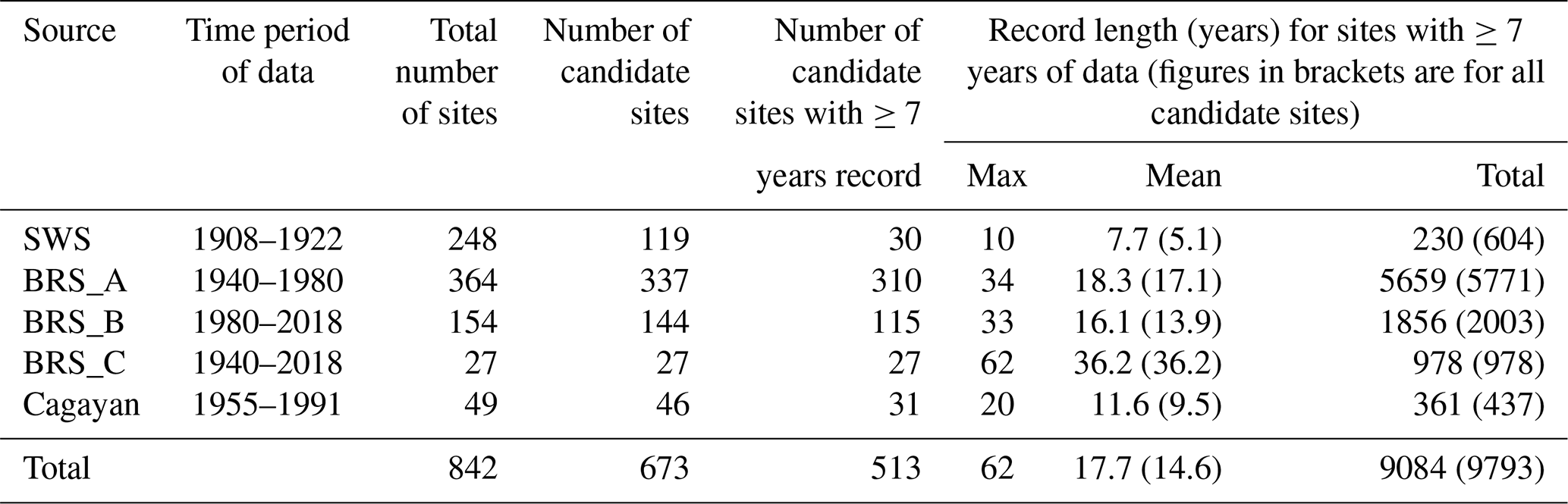
Daily mean river discharge data were collated from 842 sites (Table 1) reported by three sources. The first, “SWS” data set, comes from four volumes of the “Surface Water Supply of the Philippine Islands” (Irrigation Division, 1923–1924) that contain rating curves and daily flow measurements over the period 1908–1922. Water level measurements were made at constructed weirs, and rating curves were computed using discharges obtained by the velocity-area method. Rating information is supported by detailed information on the measurement site, bank and bed characteristics, and river channel stability. Data from 248 SWS stations across the country (Fig. 1) were used. The second data set (“BRS”) was initially managed by the Bureau of Research Standards, later being transferred to the Bureau of Design, also under the Department of Public Works and Highways (DPWH). The BRS data set (Fig. 1) is in three parts: BRS_A contains 364 gauging sites with data in the period 1940–1980; BRS_B has another 181 sites with data from 1980 onwards. BRS_C includes 27 of the sites from BRS_A and BRS_B that are either at identical locations or are sufficiently close (within a few km, without any significant tributaries in between) to allow for their records to be combined. This produces a maximum record length of 62 years. Some of these sites had automated water level sensors, but most sites had a gauging structure at which manual observations were made three times per day. Rating curves were obtained by velocity-area gauging. The source of the third data set (“Cagayan”) is the “Feasibility Study of the Flood Control Project for the Lower Cagayan River in the Republic of the Philippines” produced by Nippon Koei Co. and Nikken Consultants Inc. in collaboration with the DPWH in 2002 (Nippon Koei, 2002). This study only considers the Cagayan watershed, northern Luzon, the largest catchment in the Philippines. Out of 78 gauging stations in the watershed, 48 stations (Fig. 1) were used in this study since some of the stations only reported gauge height data and others had a lot of gaps. Daily mean water level data were recorded from 1955 to 1991 and converted to discharge using rating curves (details not reported; Nippon Koei, 2002).

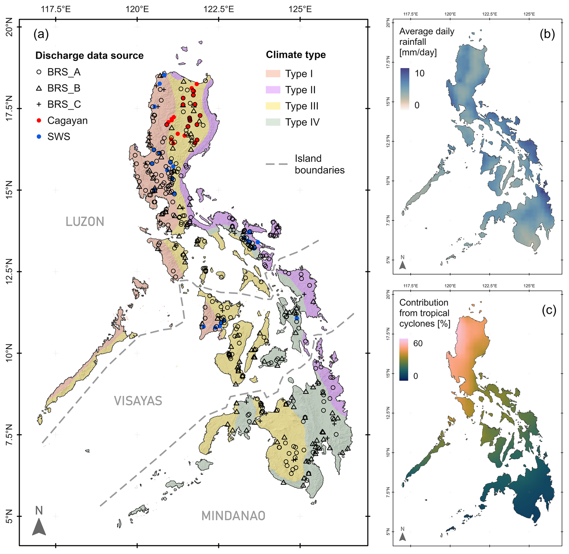
Figure 1 (a) Locations of gauging sites from the data sources used in the analysis ($n=\mathrm{466};$ Table 2). The background map (after Tolentino et al., 2016) shows elevation shading overlain by the four climate types that have been identified for the Philippines (Coronas, 1920). (b) Mean daily rainfall (after Bagtasa, 2017). (c) Proportion of annual rainfall generated by tropical cyclones (after Bagtasa, 2017). The climates can be summarised as in Ibarra et al. (2021): type I – distinct wet and dry seasons; type II – no distinct dry season and relatively high rainfall; type III – lower overall rainfall with short dry and wet seasons; and type IV – reasonably even distribution with lower total rainfall.

Table 1 Summary of available discharge data sets. Candidate sites are sites retained after removing sites with no or poor rating or indeterminate locations. Record length is the number of years for which reliable annual maximum flow estimates exist after removal of erroneous data.

The data were initially filtered to remove sites with very short records (<7 years), those with inadequate rating between water level and discharge, and those from the SWS data set where the gauging site location could not be reliably determined. The Philippines has four distinct climate types (Coronas, 1920), as shown in Fig. 1. For convenience, hydrological data are often reported for 15 administrative regions (Fig. S1), and we use this regionalisation to consider whether there is variation in flood hydrology across the country.

3 Analysis methods

3.1 Curve fitting for annual daily maximum flows

The maximum flows in each calendar year were extracted from the daily flow data and fitted to three distributions: (1) generalised logistic distribution (GLO) (Kjeldsen and Jones, 2006; Kjeldsen, 2013); (2) Weibull; and (3) log-Pearson Type III (LPIII). The median annual flood (Q_med) was used as the index flood, rather than the mean, to minimise the effect of outliers in the data (Kjeldsen and Jones, 2006), and the parameters of the distributions were estimated using L-moments (Hosking, 1990; Hosking and Wallis, 1997). L-moments are linear combinations of probability-weighted moments, and the GLO distribution uses ratios between the first three L-moments, l₁, l₂, and l₃, to define the L-CV (coefficient of variation) t₂ and L-Skewness t₃ as:

$$\begin{array}{}\text{(1)}& t_{\mathrm{2}}=l_{\mathrm{2}}/l_{\mathrm{1}}{t}_{\mathrm{3}}=l_{\mathrm{3}}/l_{\mathrm{2}}.\end{array}$$

The GLO is a three-parameter distribution, which has location, scale, and shape parameters. The location (ξ) is the median of the distribution. The shape (κ) and scale (β) parameters are estimated from the L-moment ratios (Eq. 1) as:

$$\begin{array}{}\text{(2)}& \widehat{\mathit{\kappa }}=-t_{\mathrm{3}}\mathit{\beta }={\displaystyle \frac{t_{\mathrm{2}}\widehat{\mathit{\kappa }}\sin \left(\mathit{\pi }\widehat{\mathit{\kappa }}\right)}{\mathit{\pi }\widehat{\mathit{\kappa }}\sin \left(\widehat{\mathit{\kappa }}+t_{\mathrm{2}}\right)-t_{\mathrm{2}}\sin \left(\mathit{\pi }\widehat{\mathit{\kappa }}\right)}},\end{array}$$

where $\widehat{}$ indicates an estimate of the distribution parameter. Further details on L-moments and their application to distribution fitting are provided by Hosking and Wallis (1997) and Asquith et al. (2017). The GLO distribution can be used to calculate a flood, Q_T, with a recurrence interval of T years as

$$\begin{array}{}\text{(3)}& Q_T=\mathit{\xi }\left[\mathrm{1}+{\displaystyle \frac{\mathit{\beta }}{\mathit{\kappa }}}\left(\mathrm{1}-(T-\mathrm{1}{)}^{-\mathit{\kappa }}\right)\right]=\mathit{\xi }{z}_T,\end{array}$$

where z_T is the “growth curve” at T. The Weibull and log-Pearson Type III distributions are also three parameter distributions, described fully by Asquith et al. (2017) and Hosking and Wallis (1997) who define the relevant L-moments and parameter calculations. The Gringorten (Cunnane, 1978) plotting position (Eq. 4) was used,

$$\begin{array}{}\text{(4)}& x_i=(i-\mathrm{0.44})/(n+\mathrm{0.12}),\end{array}$$

where x_i is the ith quantile of the distribution, i is the rank of the annual maximum flood in a given year, and n is the total number of years in the record. This method allows for the estimation of an event with a return period of up to 1.79n+0.2 years (Stedinger et al., 1993). Figure 2 shows typical data sets and curve fits.

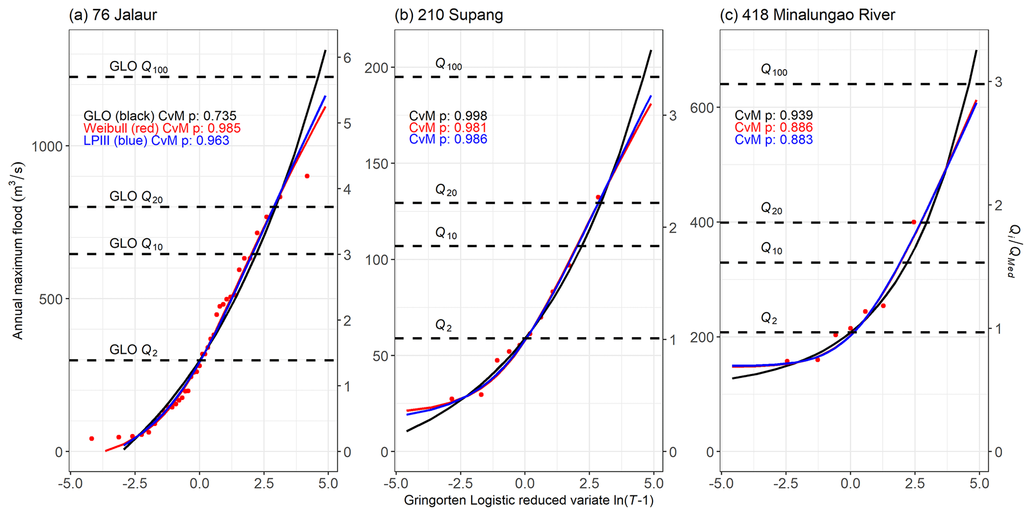
Figure 2 Selected annual maximum flood data and curve fits. Red points are data. Fitted curves are generalised logistic distribution (black), Weibull (red), and log-Pearson III (blue). Cramér–von Mises p values are shown. Left axes are flood magnitude (m³ s⁻¹), and right axes scale this by the median annual flood at each site. Values of 2, 10, 20, and 100 year recurrence interval floods are indicated and calculated using the GLO method. (a) Site 76, Jalaur (Lat: 11.1195°; Long: 122.5386°; Area: 210 km²; BRS_C data set; 37 years of data; best-fit curve: Weibull); (b) Site 210, Supang (Lat: 17.0073°; Long: 120.9086°; Area: 56 km²; Cagayan data set; 10 years; GLO); (c) Minalungao (or Sumacbao) River (Lat: 15.3430°; Long: 121.0794°; Area 309 km²; SWS data set; 7 years; GLO).

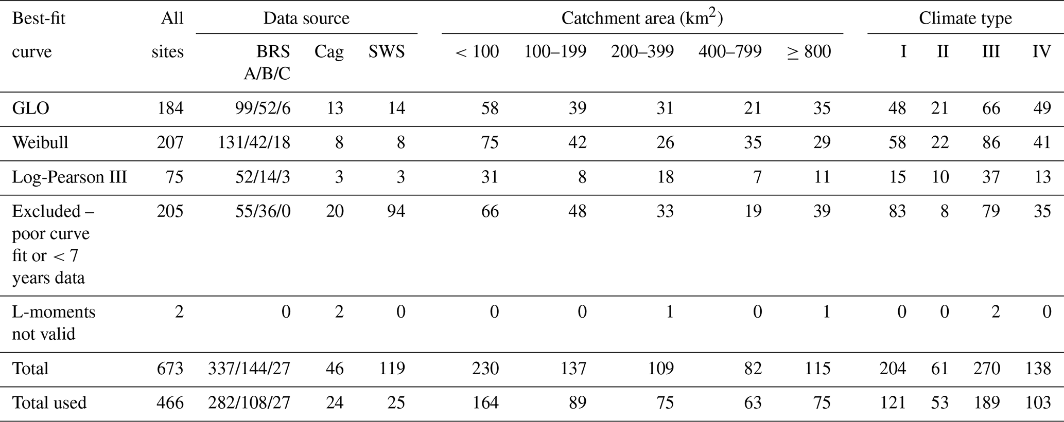
Analysis was undertaken in R (R Core Team, 2021), using the package lmomco (Asquith, 2020) to derive the L-moment estimates, to fit the distributions and to calculate their significance. Of the 513 sites with records of at least 7 years' length (Table 1), the minimum required for L-moment calculation, two had invalid L-moments and therefore were excluded from further analysis. For the remaining 511 sites, goodness-of-fit between the data and the three distributions was assessed using the Cramér–von Mises (CvM) test (Asquith, 2020). Such goodness-of-fit tests are unable to definitively identify the best distribution to use or if any of the distributions are adequate (Asquith, 2020), particularly with relatively short records, as used here. Rather, the CvM p values provide an indication of the performance of the three distributions. The annual maximum series and the three curve fits were inspected for each site, and those with visually very poor fits were excluded. Mostly, these excluded sites corresponded with low CvM p values, although this was not always the case. The median CvM p value for best-fit curves was 0.93. The distribution (GLO, Weibull, or log-Pearson Type III) with the highest p value from the CvM test was used to provide Q_x estimates for the site. This screening process led to the elimination of a further 45 sites from the data set, leaving 466 that were further analysed. The distribution of the best-fit curves (Table 2) does not show systematic differences between data source, catchment area, or climate type (Table 2).

Table 2 Best-fit curves with highest Cramér–von Mises test p value. A total of 207 sites were excluded from the analysis – two due to L-moments not being valid and the remainder due to having short records (<7 years) or a poor curve fit, based on the p value and visual inspection.

Values of Q₂, Q₁₀ and Q₁₀₀ were calculated from the fitted curves, although the lengths of available records mean that estimates of Q₁₀₀ are subject to significant uncertainty. Towards the high flow end of the data, the Weibull and log-Pearson Type III curves are usually very similar, with the GLO curve typically being steeper and more curved (Fig. 2), providing higher flow estimates for high recurrence intervals (Q₂₀ to Q₁₀₀) than the other two curves and often slightly lower estimates of Q₂ and Q₁₀. Ratios between flow estimates from different curves (Fig. S2) show this pattern: mean ratios between estimates from the GLO and Weibull distributions are Q_2GLO $/$ Q_2Wei=1.07 (range 0.99–3.48), Q_10GLO $/$ Q_10Wei=0.92 (0.70–1.00), and Q_100GLO $/$ Q_100Wei=1.09 (0.42–1.15). Equivalent ratios for the GLO and log-Pearson Type III curves are Q_2GLO $/$ Q_2LPIII=1.10 (1.00–4.27), Q_10GLO $/$ Q_10LPIII=0.91 (0.55–0.99), and Q_100GLO $/$ Q_100LPIII=1.09 (0.36–1.15). These ratios show some systematic differences between the distributions (Figs. 2 and S1) and suggest that the choice of distribution influences flow estimates.

Estimating uncertainty in the Q_x estimates is not straightforward (Kjeldsen, 2013; Kjeldsen and Jones, 2004) and reflects variability in the index flood, in the growth curve, and in covariance between the index flood and the growth curve (Kjeldsen and Jones, 2004). For a single site, the factorial standard error for the GLO distribution, fse, is defined as (Kjeldsen, 2013):

$$\begin{array}{}\text{(5)}& \mathrm{fse}=e^{\left(\frac{\mathrm{2}\mathit{\beta }}{\sqrt{n}}\right)}.\end{array}$$

Derivation of Eq. (5) relies on approximations that limit the reliability of the equation when n≤20 (Kjeldsen, 2013). On account of this, fse values were calculated only for records of at least 20 years' length, all but one of which come from the BRS data sets (Table 1).

Growth curves were calculated for each of the 466 sites (Table 2) using Eq. (3) and equivalents for the Weibull and log-Pearson Type III distributions, over the range of $-\mathrm{3.5}\le \ln (T-\mathrm{1})\le \mathrm{5.0}$, i.e. return period T in the range 1 to 149 years. Curves were standardised by dividing discharge by the median annual flood recorded at each site.

Combined growth curves using data from sets of catchments that are adjacent or have similar properties (e.g. catchment area) can be used to provide estimates of the magnitude of floods at specified recurrence intervals, given an initial value of Q_med. There are several ways to construct such pooled growth curves for (i) each of the administrative regions of the Philippines; (ii) each of the four climate types (Fig. 1); and (iii) catchments of different areas, as identified in Table 2. Firstly, the curves from each site within any of these groups can be combined by calculating their mean, mean weighted by record length, or median (Figs. S3–S5). Secondly, the data can be amalgamated for all sites within each group and GLO curves fitted to the pooled data. The median and weighted mean methods lead to under-estimation of the longest recurrence interval floods (Figs. S3–S5), whereas both the mean of the best-fit curves from each site and the GLO curves fitted to the amalgamated data increase more rapidly at long recurrence intervals. Note that the variability between sites within a region (or climate type or within catchments of similar area) provides an indication of the uncertainty to be expected when using regionalised curves.

3.2 Predicting high magnitude floods from catchment properties

The values of Q_T provided by the best-fit curves for each site individually determined above were correlated with catchment properties. These catchment properties, precipitation, and land use were derived from a range of data sources. Table 3 summarises the variables used and provides a comparison with the FEH method (Kjeldsen et al., 2008). Note that much of the data used are not contemporary and significant changes in some variables, particularly land use but potentially also precipitation (Bagtasa, 2017), may have occurred since the SWS data were collected in the early 20th century.

Table 3 Variables used in the flood prediction analysis.

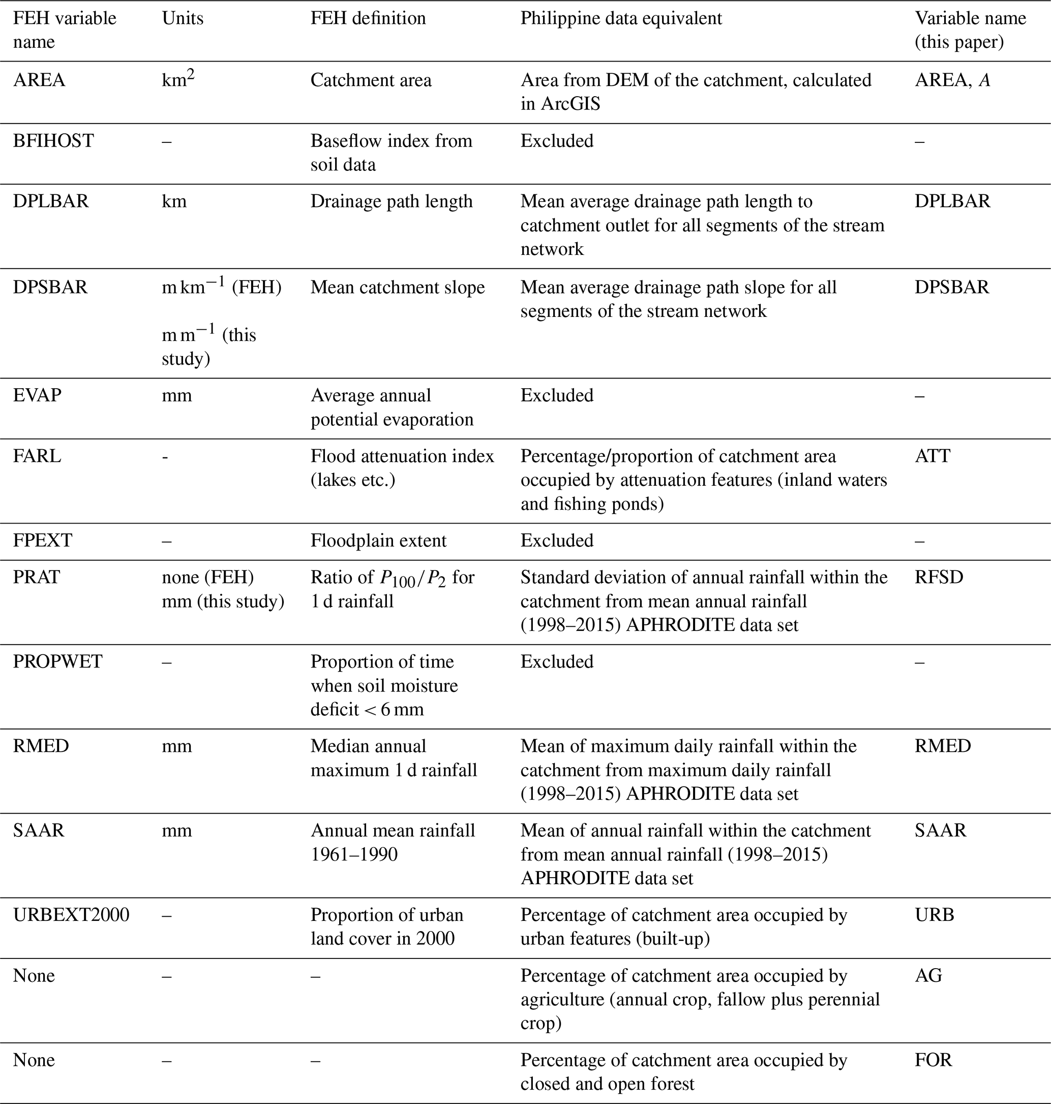
National-scale catchment physical properties for the Philippines were previously calculated and are available as an open-access geodatabase (Boothroyd et al., 2023). In brief, topographic analysis was undertaken using a digital elevation model (DEM) acquired in 2013 with a 5 m spatial resolution and 1 m root-mean-square error vertical accuracy (Grafil and Castro, 2014). The DEM was resampled to a 30 m spatial resolution in ArcGIS due to processing constraints. Here, AREA, DPLBAR, and DPSBAR were extracted from the geodatabase. Rainfall data were from the end-of-the-day adjusted version of the APHRODITE data set (V1901, Yatagai et al., 2012). Land use variables (ATT, URB, AG, FOR) were taken from the National Mapping and Resource Information Authority (NAMRIA) 2010 land cover data set (https://www.namria.gov.ph/, last access: 15 October 2025).

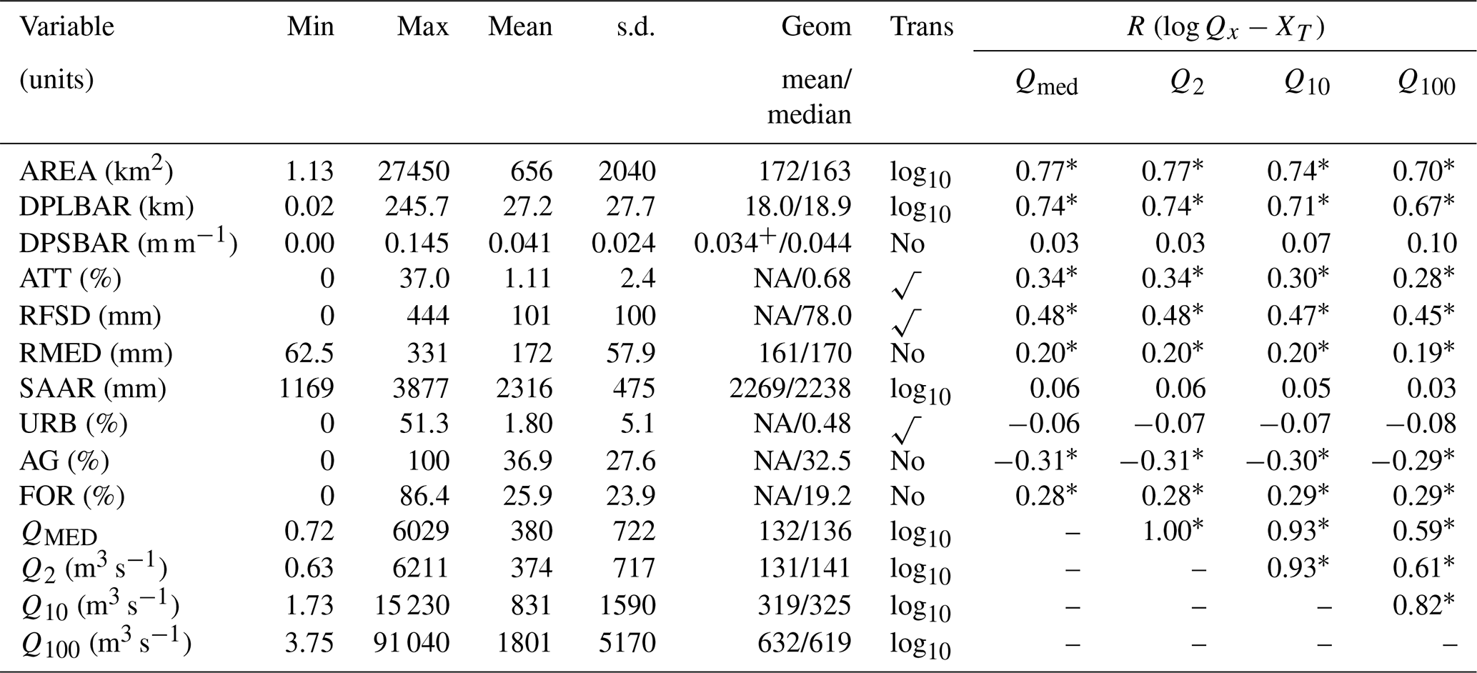
Each of the variables listed in Table 3, together with the estimates of Q₂, Q₁₀, and Q₁₀₀, was tested for normality and transformed as required (Table 4). log ₁₀ transformation was used as the default, most variables being moderately positively skewed, with square-root transformation for two land use (areas of attenuation features and urban land use) and one rainfall (standard deviation of rainfall) variables that contained numerous zero values. Cross-correlation plots and matrices of the transformed variables, where relevant (Fig. S7), show expected autocorrelation between climate variables and no significant non-linear relationships elsewhere in the predictor variables. Note (Table 4) that mean annual rainfall (SAAR) is poorly correlated with each of the Q_x measures.

Table 4 Summary statistics for variables used in the flood prediction analysis (466 sites). All values are in original units, prior to transformation (Trans). Land use variables expressed as % were converted to proportion (0–1 scale) for analysis. Correlation coefficient, R, significance: ^* p<0.01. Geometric mean (Geom mean) shown for variables with no zero values. ⁺ One slope of 0.0 was excluded when calculating geometric mean. X_T = transformed value of variable X. NA = geometric mean not able to be computed due to zero values.

4 Results

4.1 Validity of L-moment calculations

The L-moment ratio diagram (Figs. 3 and S6) shows the relationship between L-skew and L-kurtosis differentiated by catchment area and the optimal best-fit curve. Sites where each of the distribution types fits the data best cluster close to the theoretical relationships for each of those distributions as expected. Neither climate type (Fig. 3), data source, catchment area, nor record length (Fig. S6) shows significant segregation on the L-moment diagram. Consequently, the 466 retained sites are considered as a single data set in subsequent analysis.

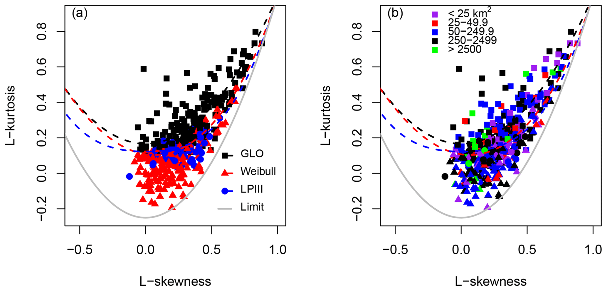
Figure 3 Relationships between L-skewness and L-kurtosis compared with theoretical curves (Hosking and Wallis, 1997). Data are classified by (a) best-fit curve and (b) catchment area. Panel (a) shows segregation between sites with different best-fit curves, with higher positive L-kurtosis associated with the GLO curve and low to negative L-kurtosis associated with the sites where the Weibull curve fits the data best. Panel (b) shows overlap between the best-fit curve type and catchment areas with no clustering of different-sized catchments. Colours indicate catchment areas, as shown at the top of the figure, and symbol shapes (as shown in the legend of panel a) indicate best-fit curves. Figure S6 plots the data classified by climate type, length of record, and data source; in all cases, there is no segregation according to the classifying variable.

Only for sites (N=71) that had at least 20 annual maxima and for which the GLO distribution provided the best fit to the data, was it possible to compute the factorial standard error (fse) using Eq. (5). The values of fse range from 1.03 to 1.32, with mean = 1.18. It is noted that uncertainty will be greater for sites with records of less than 20 years.

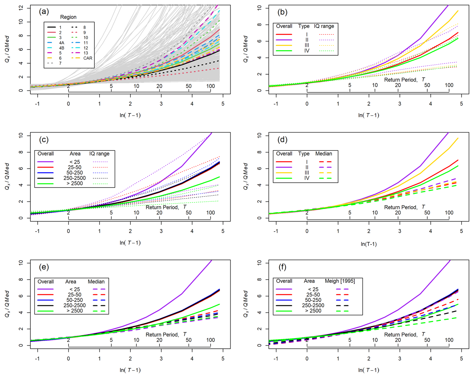
Figure 4 Dimensionless growth curves. (a) Individual curves (GLO, Weibull, or log-Pearson Type III, according to which produced the highest p value in the Cramér–von Mises test) for 466 sites, overlain by pooled GLO curves for each region. (b) GLO curves fitted to data pooled from all sites in each climate type; IQ range lines represent the interquartile range (25th and 75th percentiles) of the curves for individual sites within each climate zone. (c) GLO curves fitted to all data within bins of catchment area, with interquartile ranges from individual sites shown. (d) Comparison of GLO curves fitted to all data within each climate zone and the median value from curves fitted to individual sites within that zone. (e) Comparison of GLO curves fitted to all data from sites within each catchment area bin and the median value from individual sites within that bin. (f) Overall GLO curves for each catchment area bin and adjusted equivalent curves from Meigh (1995). Adjustment was necessary because Meigh (1995) used the mean annual flood as the index flood rather than the median. See the text for details.

4.2 Regional annual maximum daily flow growth curves

Growth curves for all sites (Fig. 4a) show considerable variability within and between regions, reflecting the number, length, and quality of available data records as well as catchment properties. To assess variation across the country, we use the administrative division of the Philippines into 15 regions (Fig. S1), which are aligned to hydrological and topographic patterns (Fig. 1). Different climate zones (Fig. 4b) and catchment areas (Fig. 4c) indicate some grouping that may form the basis for hydrologic regionalisation. Climate types II and III plot higher than the others (Fig. 4b), although the median growth curves for all four climate types are very similar (Fig. 4d). The pooled data provide steeper growth curves, reflecting the larger data series used and the increasing influence of large events in these larger samples. Consequently, the pooled data curves match high percentiles of the individual curves (shown by plotting close to or sometimes outside of the 75th percentile limits, as shown in Fig. 4b and c). The steeper curves for pooled data are also seen when grouped according to catchment area (Fig. 4e). Small (<25 km²) catchments plot separately from all larger areas, and there is little differentiation between any larger catchments. This contrasts with Meigh's (1995) results, which suggested a steady decrease in $Q_x/Q_{\mathrm{mean}}$ as the catchment size increased.

4.3 Flood estimation equations

4.3.1 Flood prediction from catchment area and rainfall

The correlations in Table 4 show that catchment area alone provides the most significant prediction of flood magnitude. Drainage path length (DPLBAR) is an equally good predictor, as path length is correlated with catchment area (Hack's law; Rigon et al., 1996). However, R² for catchment area and DPLBAR is in the range 0.45–0.6, so there is potential for additional variables to improve flood magnitude prediction. Initially, the rainfall variables were introduced to multiple regression relationships to account for the volume of water entering catchments as catchment area × rainfall. Tables 3 and 4 show two relevant rainfall variables: SAAR, the mean annual rainfall, and RMED, the maximum daily rainfall, which serve as a measure of the magnitude of rainfall extremes that may be expected to be correlated with flood peaks.

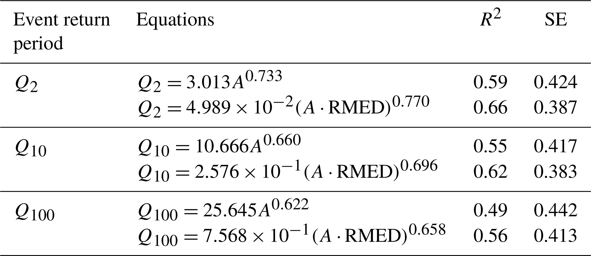
Equations using catchment area alone (Table 5) provide R² values between 0.49 (Q₁₀₀) and 0.6 (Q₂). These rise to 0.55–0.65 when area is multiplied by RMED (Table 5). P₉₉, the 99th percentile of daily rainfall, produces equations that fit the data equally well as RMED.

Table 5 Best-fit equations for the data set covering the whole of the Philippines (n=466). SE = standard error of residuals.

The residuals from the equations using A⋅MED as the predictor were examined for effects of data source, climate type, or region (Fig. 5). One-way ANOVA indicates significant differences between regions for Q₂, Q₁₀, and Q₁₀₀, with regions 7 (p=0.003; 0.0043; 0.026, respectively), 11 (p=0.012; 0.001; 0.005), and 12 (p<0.001 for all Q_x) being significantly different for all three return periods, region 3 (p=0.02; 0.02) for Q₁₀ and Q₁₀₀, and region 9 (p=0.02) for Q₁₀₀ only. Differences between climate types are only significant for Q₁₀ and Q₁₀₀, in both cases Type IV being significantly different from the others (p<0.01). For data source, significant differences are noted for Q₂ and Q₁₀, in both cases due to BRS_B (p=0.006 for both) and the early 20th century SWS (p<0.001 and 0.014 for Q₂ and Q₁₀, respectively) data sets. While these results suggest possible benefits from subdividing the data to produce predictive equations, inspection of Fig. 5, the boxplots, and ANOVA results all show considerable inter-group variance. Hence, the alternative approach of introducing additional variables to the analysis is considered as the next stage of the analysis, before regionalisation is considered in Sect. 4.3.3.

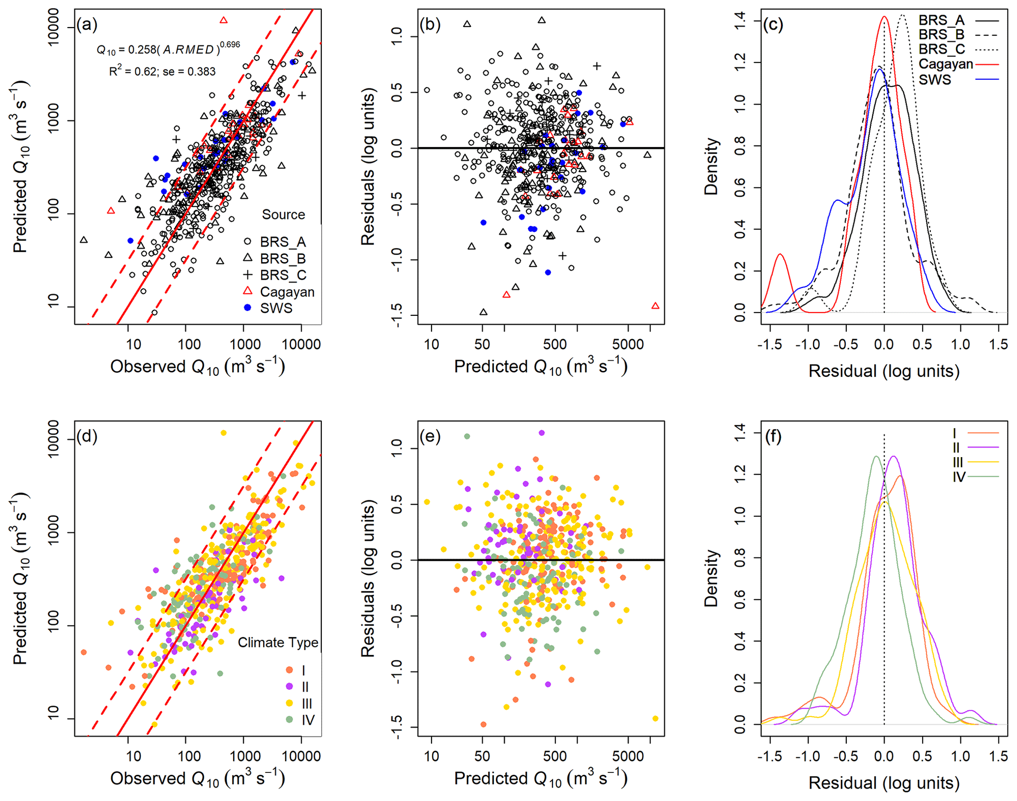
Figure 5 Observed values, predictions, and residuals for Q₁₀ as a function of catchment area (A) multiplied by median daily maximum rainfall (RMED). (a–c) Stratified by data source and (d–f) by climate type. Panels (a) and (d) show predicted vs. observed values with 1:1 (solid) and 1:2 and 2:1 (dashed) lines. Residuals in (b) and (e) are normally (Gaussian) distributed and show no systematic variation with predicted Q₁₀. Density plots of residuals in (c) and (f) confirm the absence of systematic variation with data source and climate type. Equivalent figures for Q₂ and Q₁₀₀ are provided in the Supplement (Figs. S8 and S9).

4.3.2 Comprehensive stepwise regression prediction

Stepwise regression yielded equations (Table 6) with between three and six significant (p<0.05) predictors but overall R² values of 0.68, 0.63, and 0.57 for Q₂, Q₁₀, and Q₁₀₀, respectively. The modest improvements in R² associated with these additional variables suggest that there is limited value in using these complex equations for flood magnitude prediction.

Table 6 Best-fit stepwise equations for the data set covering the whole of the Philippines (n=466). SE = standard error of residuals.

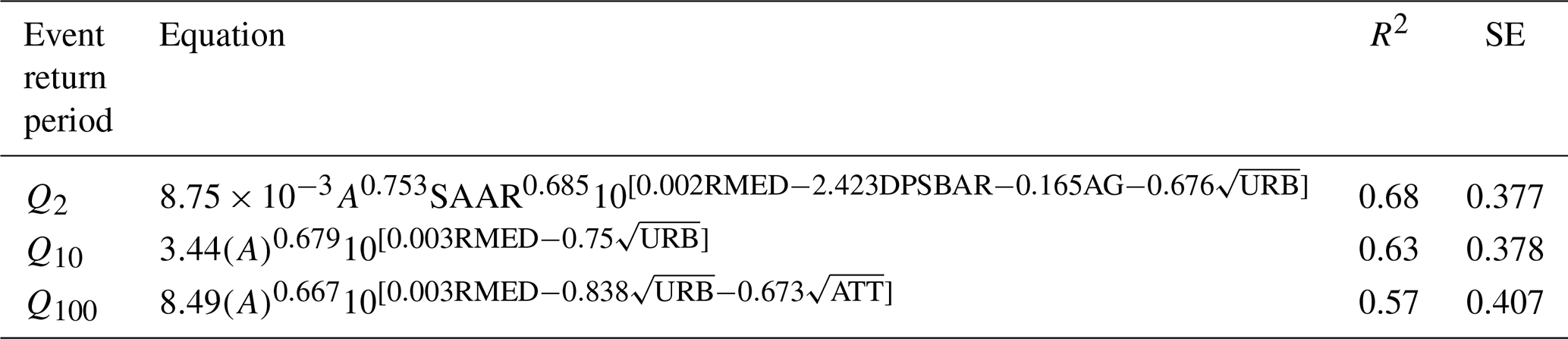
This limitation is enhanced by consideration of the variables in the equations. Each equation contains land use variables (ATT, URB, and AG) that are determined from modern conditions. The relevance of these values to historical data is uncertain given historic and contemporary land use change across the Philippines. Their inclusion in equations for all three return periods does suggest that land use may play a significant role in flood magnitude. In all three cases, catchment area A enters the equation first, followed by RMED. R² values after each of these steps for Q₂, Q₁₀, and Q₁₀₀ are A: 0.59, 0.55, and 0.49 and A and RMED: 0.66, 0.62, and 0.55. Adding further variables (Table 6) improves R² by ≤0.02; hence, only catchment area (A) and median annual maximum daily rainfall (RMED) are considered necessary for developing predictive equations. Whether these two predictors are added sequentially or are multiplied together (Table 5) does not affect overall model performance (note that the RMSE values quoted in the equations are for the transformed variables). Subsequently, the product A⋅RMED is used as a single measure of flood event rainfall volume across the catchments.

4.3.3 Regionalisation of predictive equations

The dimensionless growth curves (Fig. 4a), inspection, and ANOVA of regression residuals suggest that regionalisation may be able to improve predictive equations. Although the growth curves also show some segregation between climate types, this is not found to be a significant cause of variation in the residuals from predictive equations. Fitting equations to each region separately (Fig. 6a) yields improvement in R² and residual standard error for some regions, but this is inconsistent. The regional equations suggest that some grouping of regions may be beneficial.

Three ways of dividing the 15 regions into groups were considered: (a) classification by visual inspection of the growth curves, (b) K-means cluster analysis of the intercepts (a) and gradients (b) for regression equations (Fig. 6a), and (c) the regionally contiguous groups used by Meigh (1995). Each grouping was tested for Q₂, Q₁₀, and Q₁₀₀ predictions. Results were consistent between these return periods, and results for Q₁₀ are given in Table 7 (see the Supplement for Q₂ and Q₁₀₀ results).

Table 7 Equations for different groups of regions. Results for Q₁₀ are presented. Meigh (1995) did not include regions 13 or CAR, so the total number of sites in the three contiguous regional groups is 431.

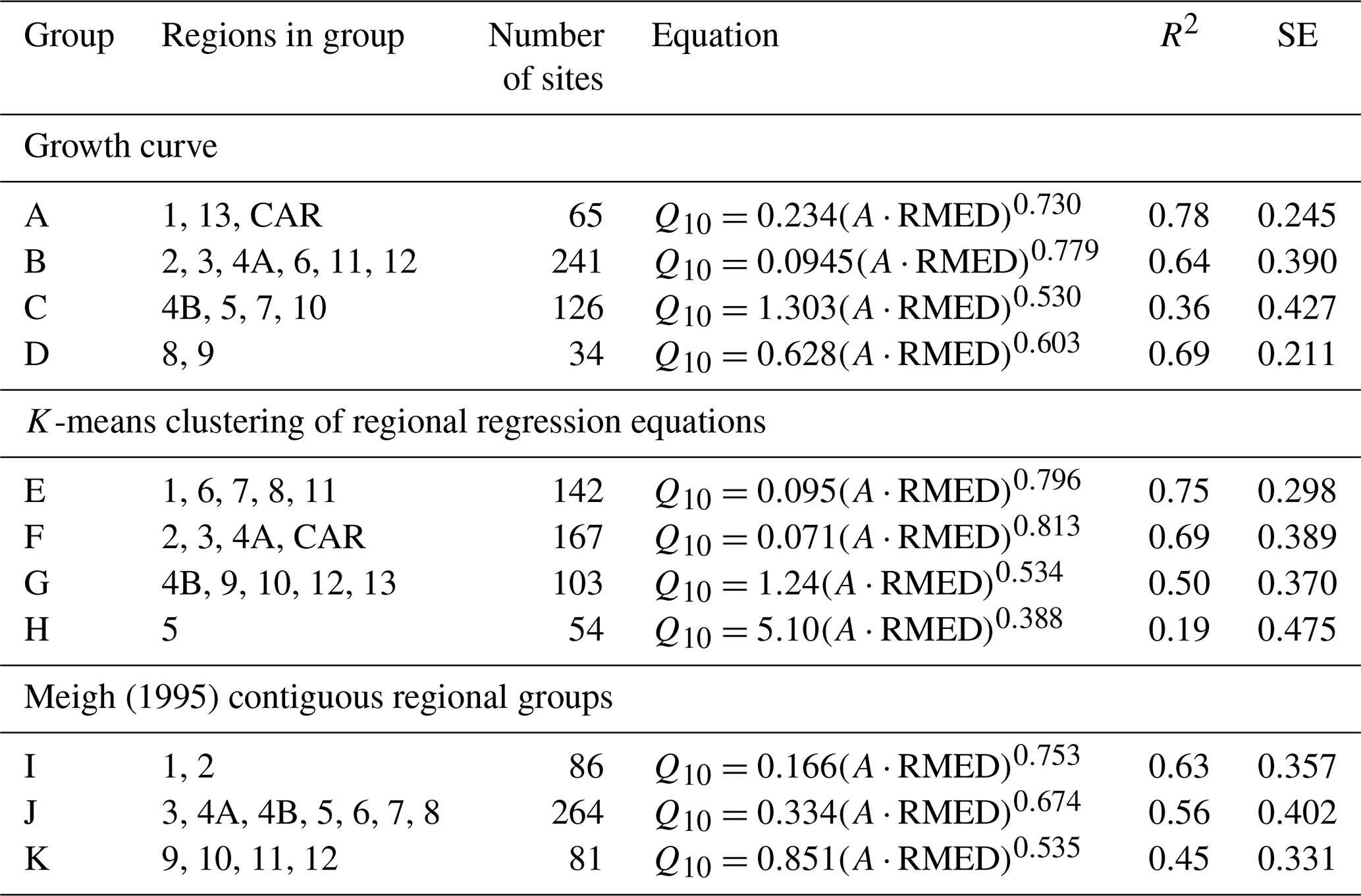
The R² and standard errors of residuals in Table 7 are compared with the combined results for all regions in Table 5 (R²=0.62; SE = 0.383). Weighting both the R² and residual error values by the number of sites in each group/region suggested that for Q₂, Q₁₀, and Q₁₀₀ the highest R² values are those obtained using the overall regressions on the full data set (Table 5). The residual standard errors are slightly lower when obtained from the 15 individual regional curves (0.36, 0.35, and 0.37 for Q₂, Q₁₀, and Q₁₀₀, respectively) than from the overall regressions (0.39, 0.38, and 0.41). However, these differences are small, and there is insufficient evidence to justify the use of curves either for individual regions or for groups of regions.

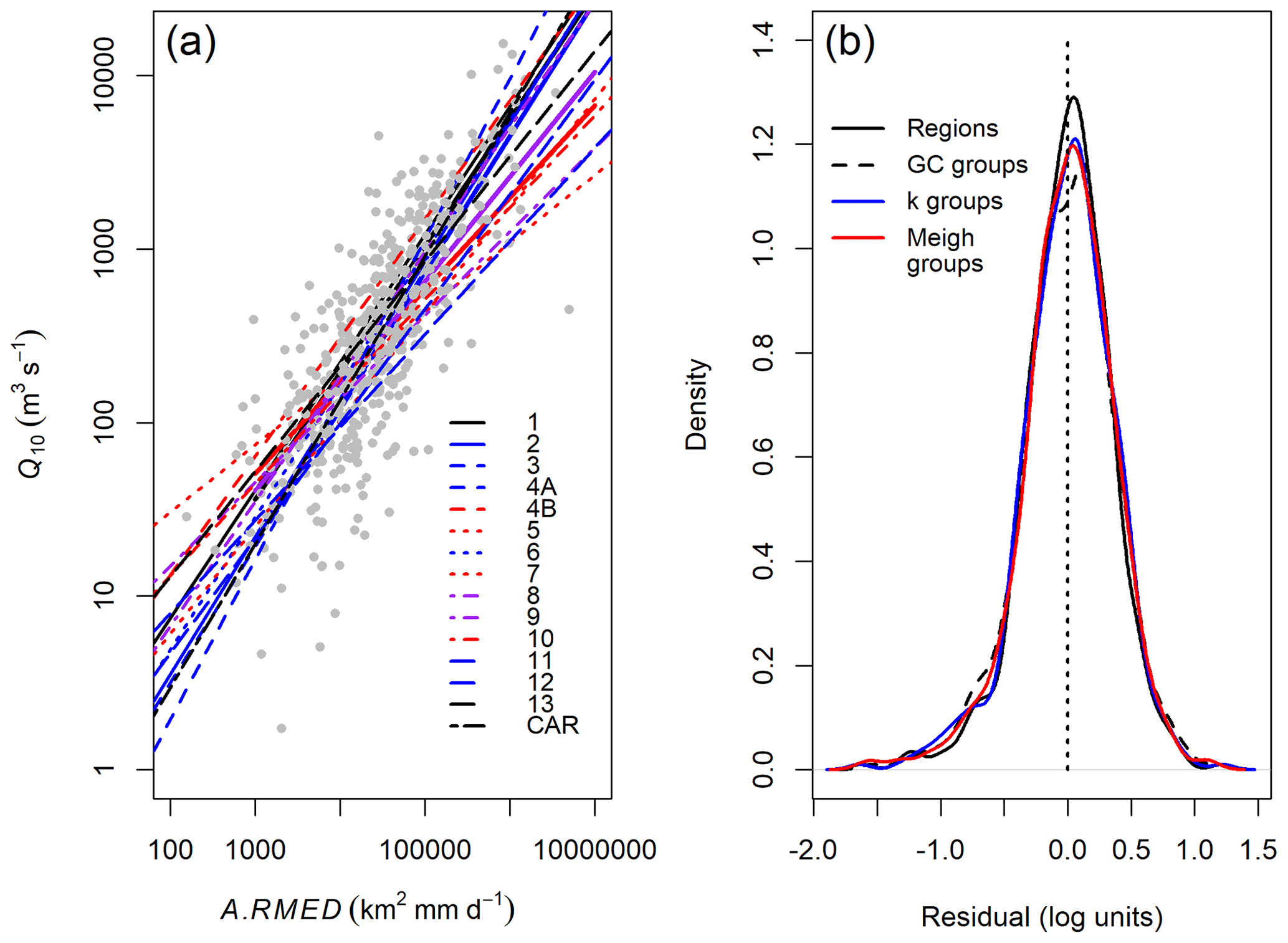
Figure 6 (a) Regression curves for each region in the form $Q_{\mathrm{10}}=a(A\cdot \mathrm{RMED}{)}^b$. Curves are grouped according to growth curve shapes (Table 7): group A (black), B (blue), C (red), and D (purple), and bold lines represent the regional curves given by the equations in Table 7. (b) Probability density functions for residuals from the individual regional curves in panel (a) and the three groupings of regions in Table 7 (GC = growth curve; k = k-means). Note the similarity in the distributions of residuals, although those for the individual regions are clustered slightly more closely around the mean than those from the grouping methods.

4.3.4 Spatial distribution of flood magnitudes and residuals

The spatial distribution of calculated specific flood magnitudes (Q_xx divided by catchment area A) (Fig. 7a) shows a concentration of higher values through the central Philippines, with relatively lower values in NE Luzon and across Mindanao in the south. The underlying annual rainfall map shows a general decline from east to west, and some of the highest rainfall areas are associated with high $Q_{xx}/A$ values, for example, in the Bicol region. Residuals from the overall equations (Table 5) do not show strong regional trends, although there are clusters of positive and negative residuals in different regions. The residuals are not correlated with catchment area ($R=-\mathrm{0.04}$; p=0.39) and are correlated only weakly with annual rainfall (R=0.15; p<0.001). However, there is a significant positive correlation between residuals and specific flood magnitude ($R=\mathrm{0.62};$ $p<\mathrm{2}\times {\mathrm{10}}^{-\mathrm{16}}$), with only negative residuals for $Q_{\mathrm{10}}/A<\mathrm{0.46}$ and only positive residuals when $Q_{\mathrm{10}}/A>\mathrm{6.4}$. These results are replicated for Q₂ and Q₁₀₀, with significant correlations of 0.6 ($p<\mathrm{2}\times {\mathrm{10}}^{-\mathrm{16}}$) for both $Q_{\mathrm{2}}/A$ and $Q_{\mathrm{100}}/A$.

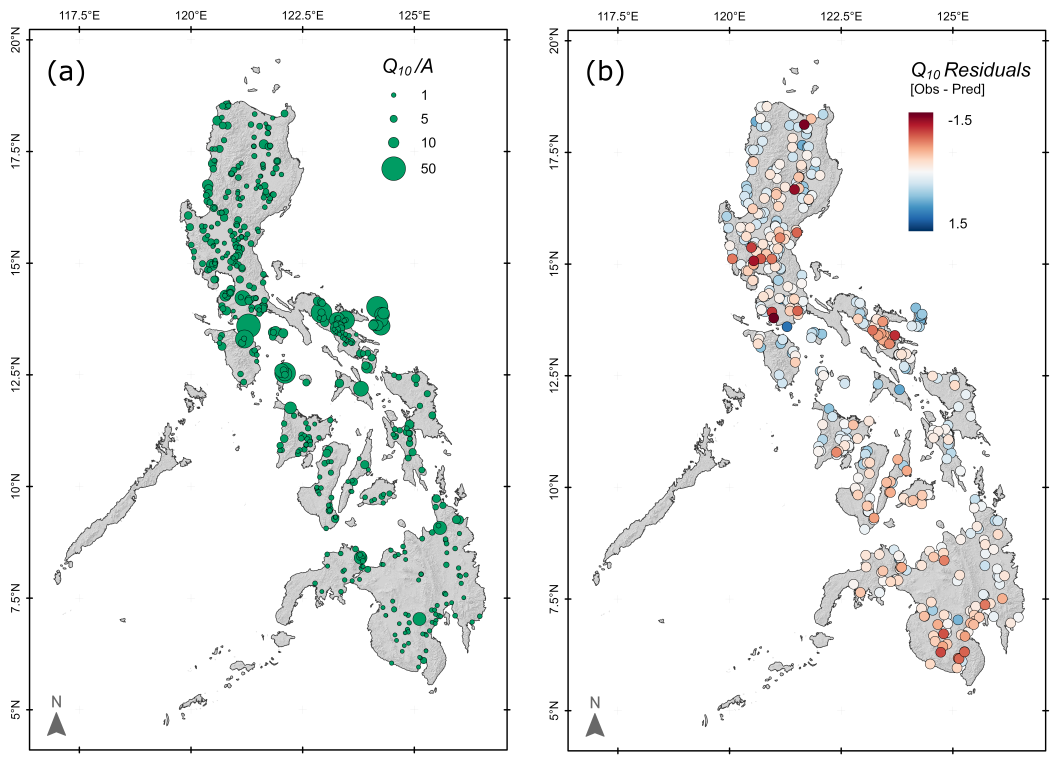
Figure 7 (a) Specific 10 year flood discharge ($Q_{\mathrm{10}}/A$), showing generally higher values in the central Philippines and southern Luzon and lower values across Mindanao. (b) Residuals (in log ₁₀ units) from Philippines-wide (Table 5) equations for Q₁₀. Note the absence of regional trends, although there are some sub-regional clusters of both positive and negative residuals.

5 Discussion

5.1 Design equations for the Philippines

5.1.1 Data availability and quality

Flow data were combined from four data sets that are partly independent, having been collected by different agencies and using different methods, but they overlap significantly in collecting data at the same or nearby locations. Catchment properties, such as area and gradients, were derived from a high-resolution DEM that covers the whole of the Philippines. Although some station locations are ambiguous in the data records, the locations of all stations included in the analysis have been reliably identified using the descriptions in the original data sources. Land use data rely on a single time, and no historical land use data are available. This introduces uncertainty to the analysis, especially for data collected a century or more prior to the land use data in areas that have undergone urban development or forest replacement by agriculture.

The proportions of variance in flood estimates that are statistically explained by the best-fit equations (R²; Tables 5–7) are within the range from studies in other tropical regions (Meigh et al., 1997), from 0.38 (Malawi) to 0.92 (Papua New Guinea). The relatively low R² values reflect a range of factors, including data quality and length of flow records, changing climate and hydrological conditions during the time period covered by the study, and controls over flood magnitude in these tropical catchments being influenced by hydrological parameters that are not considered in the analysis. Data quality has been assessed throughout, with sites excluded if their growth curves are based on short records or do not fit expected shapes (Tables 1 and 2). Further, there is no evidence of bias in the data, shown both by the original variables and the behaviour of residuals from the final predictive curves. For example, the best-fit curves are not biased by data source, climate type, or record length (Figs. 3, S6, S8, and S9). The residuals show neither systematic variation across these same categories (Fig. 5) nor consistent spatial dependence (Fig. 7).

Some spatial dependence is visible in Fig. 7, although attempts to produce regionally consistent predictive curves (Table 7; Fig. 6) do not improve the overall performance of the equations compared with national equations. The residuals in Fig. 7 do not correlate clearly with either total rainfall (Fig. 1b) or the relative importance of tropical cyclones in generating precipitation (Fig. 1c). Further analysis of the role of regional climate in flood generation may be able to provide some improvements to predictions, although this is complicated by ongoing climate change and potential changes in the importance of cyclonic precipitation (Bagtasa, 2017).

5.1.2 Recommended design equations

Neither the addition of further catchment variables (Eq. 6), nor regionalisation (Table 7) generated significant improvement in the predictive capabilities of the discharge equations. Hence, it is recommended that single national equations are utilised. This approach has the advantage of maximising the size of the data set used in generating the equations, particularly for the largest catchments, where the small sample size reduces confidence in the predictions in some regions. Regionally grouped equations (Table 7) can provide additional estimates of flood magnitude that may be helpful in some cases.

The recommended design equations for Q₂, Q₁₀, and Q₁₀₀ are those for the whole of the Philippines given in Table 5. Using only catchment area, A, will provide usable flood magnitude estimates, the uncertainty of which can be estimated from the residual standard errors given in Table 5. Here, we obtained RMED values from the APHRODITE database. RMED can be determined in other ways, and the sensitivity of flood predictions to changing RMED can be assessed directly. Along with catchment area, other catchment properties that provide information to contextualise the flood magnitude estimates can be obtained from an open-access database (Boothroyd et al., 2023). Utilising design equations based on catchment area alone has the advantage of simplicity of computation, but the relatively low R² values (Tables 5 and 7) obtained suggest that a simple multivariate regression approach offers only partial improvement to the predictive capability of the equations.

Being derived from a large data set, the design equations have narrow confidence intervals (Fig. S10). For use as estimators of flood magnitude, prediction intervals are required. These (Fig. S10) are of 1 order of magnitude either side of the regression lines, reflecting the scatter in the data (quantified by the standard errors of residuals in Table 5). The greatest challenge with the Philippines data lies in the relatively short data records and the sparse data from recent decades. Shorter records are associated with greater uncertainty in growth curve shape (Fischer and Schumann, 2022; Papalexiou and Koutsoyiannis, 2013) and derived flood estimates (Kjeldsen, 2013). The equations in Table 5 can be analysed to assess the relative importance of catchment area and rainfall in determining flood magnitudes, with catchment area being the predominant control. This result suggests that climate change impacts on rainfall patterns may have relatively small, but potentially locally significant, impacts on flood magnitude. Other impacts of climate change, for example, on vegetation and sediment production rates, may lead to indirect changes in flood patterns due to changes in sediment budgets and river mobility (Quick et al., 2025). Further analysis of the data, including the structure of the predictive models and the impacts of uncertainties in input data, may prove informative. However, the combination of data from different sources and the limitations in some of these data sets, as explained above in Sects. 2 and 3.2, will constrain interpretations from uncertainty analysis.

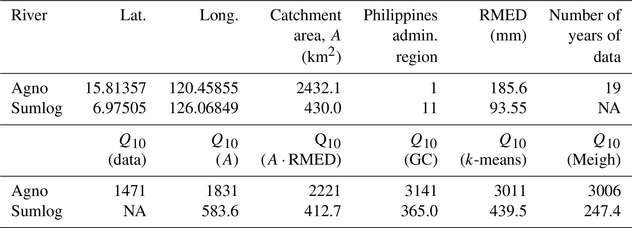
Table 8 shows sample calculations for two sites, one of which (Agno) has 19 years of annual maxima available, whereas the other (Sumlog) is ungauged. For Agno, all of the equations from Tables 5 and 6 produce higher estimates of Q₁₀ than those from the observations. The reliability of the predictive equations may be affected by this being one of the largest catchments in the Philippines. Sumlog is a smaller catchment for which no data are available. In this case, the equations provide a smaller range, with the calculations using the three regional methods (Table 7) spanning the result from the national-scale equation using A⋅MED in Table 5.

Table 8 Sample calculations for Q₁₀ using equations from Tables 5 and 6. The six Q₁₀ estimates for each site are as follows: Q₁₀ (data) from annual maxima recorded at the Agno site only; Q₁₀(A) using catchment area only – equation from Table 5; Q₁₀(A⋅RMED) using catchment area and RMED – equation from Table 5; Q₁₀ (GC), Q₁₀ (k-means), and Q₁₀ (Meigh) using equations from Table 6 for selected groups of Philippine administrative regions. NA – not available.

5.2 Comparison with other estimates

5.2.1 Comparison with similar approaches

The previous large-scale study of Philippine flood magnitude (Meigh, 1995; Meigh et al., 1997) used a smaller data set than that used here, based mainly on BRS data from before 1980, and fitted only the general extreme value distribution to the annual maxima time series. The overlap in data means that Meigh's (1995) study cannot be considered to be independent of the present analysis and so does not provide a validation of our results. Some comparison between the two studies is valuable to illustrate the effects of using an expanded data set and the GLO fitting approach (Fig. 4f). Liongson (2004) used data from 29 stations and found that Q_m=5.90A^0.763 (R²=0.65), which is consistent with results in Table 5, as Q_m lies between Q₂ and Q₁₀.

Meigh et al. (1997) presented global data although with an emphasis on tropical regions. Their best-fit equations contain few variables, often only the catchment area, with mean annual rainfall as the secondary predictor. Comparison of equations between sites revealed the expected overall pattern of higher specific discharges in more humid areas with steeper growth curves in more arid locations that have more variable rainfall, as also seen in the data of Loebis (2002). The consistency of rainfall across the Philippines leads to a clear catchment area effect (Fig. 4f) in growth curves for small (<25 km²) and large (>2500 km²) catchments, although using aggregated data shows no differentiation for catchments of intermediate sizes. Individual catchment growth curves show considerable variation within all of the catchment area bins, suggesting that caution is needed in using the aggregated curves for predictive purposes at individual sites. Figure 4 provides a range of aggregated growth curves that can be applied according to catchment area and/or climate type. The differences between the median and mean curves in Fig. 4 reflect skewness in the growth curve distributions, which is likely to result from the use of relatively short records, some of which will include long return period events thus overestimating flood magnitudes. Median curves (climate type – Fig. 4d; catchment area – Fig. 4e) can be used in flood estimation, with the associated mean values and interquartile ranges (Fig. 4b and c) giving indications of the possible variability, and hence, uncertainty, associated with these estimates.

5.2.2 Comparison with rainfall-runoff modelling

The Philippines “Nationwide Disaster Risk and Exposure Assessment for Mitigation (DREAM) Program” produced reports for major Philippine river basins (https://dream.upd.edu.ph/products/publications/index.html, last access: 19 October 2025), which included flood magnitude estimation. In the DREAM study, 24 h rainfall events with a range of return periods were calculated from data, and these events were then used to model river flows in HEC-HMS 3.5 software. Comparisons are made using catchment area equations (Table 5) for Q₁₀ and Q₁₀₀ for sites with unambiguous locations from which DREAM results are reported and for which we are able to calculate catchment areas.

Q₁₀ and Q₁₀₀ comparisons (Figs. 8a and S11) cluster around the 1:1 line of agreement. The HEC-HMS estimates exceed the predictions using catchment area at 27 of 38 sites for Q₁₀ and at 24 sites for Q₁₀₀. Mean ratios between HEC-HMS and predicted values are 1.61 for Q₁₀ and 1.76 for Q₁₀₀. The HEC-HMS results are for instantaneous flows, which will be greater than the predicted daily mean flows, with the magnitude of this difference depending on hydrograph shape and hence catchment size (Fig. 8b). Given the uncertainties in the data and predictions noted above and the limited calibration data available for the flood modelling in the DREAM project, the results shown in Fig. 8 provide confidence in both the HEC-HMS modelling undertaken for the DREAM project and the catchment area-based predictions developed herein, although results using both approaches are subject to significant uncertainty.

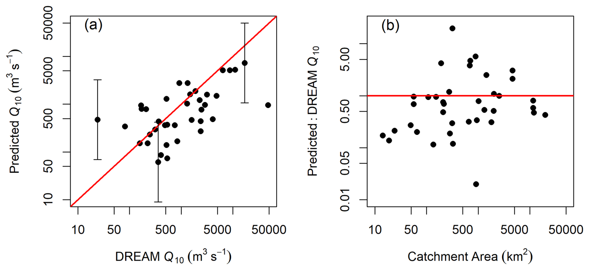
Figure 8 (a) Comparison between Q₁₀ estimates based on catchment area (Table 5) and HEC-HMS estimates from the DREAM project. The red line shows 1:1 equivalence. (b) Effect of catchment area on the ratio between Q₁₀ values from this study and the DREAM HEC-HMS modelling. The red line indicates equal Q₁₀ values from both methods. DREAM estimates are instantaneous peak flows, whereas the estimates herein are daily means. As catchment area increases, equivalence between the two methods would show the Q₁₀ ratio increasing towards 1.0, with lower values in smaller catchments in which flood peaks are shorter than 1 d duration. 95 % prediction intervals are shown for selected points in (a) to indicate the magnitude of statistical uncertainty in the predictions. These are approximated as ±2 SE, where SE is the regression standard error given in Table 5. Figure S11 presents equivalent results for Q₁₀₀.

5.3 Combining data from multiple sources

Long hydrological time series are not commonly available worldwide, with particular challenges in developing countries (Cabrera and Lee, 2020). More usually, short, discontinuous records are available, and the challenge is to make best use of these to produce regional or national design equations. Combining data from different sources and over different time periods raises several issues, including changing data gathering methodologies, climate and land use changes, and rating curve changes due to relocation of measuring sites and/or river bed morphological changes. Uncertainty in individual measurements was assessed here through careful reading of available metadata and quality control. Comparison of results from different data sources (e.g. Fig. 5a–c) shows no statistically significant differences between results from analysis for each of the data sets, thereby supporting our amalgamation of the data from different sources for aggregated analysis. The metadata available for the early 20th century SWS data include very detailed site descriptions, rating curves, assessment of site stability, and statements on data reliability from the authors (Irrigation Division, 1923–1924). Such details are rarely available, at least in accessible public records, for more recent data. The SWS reports provide useful insight into the challenges of hydrometric monitoring in the Philippines, with several sites showing evidence of channel change and frequent shifts in rating curves. Although beyond the scope of this paper, such changes in rating behaviour can be used to assess the impacts of land use and climate changes on river sediment budgets (e.g. Slater et al., 2015).

The validity of combining data is difficult to assess directly. The residuals from predictive curves (Fig. 5c) and similar disaggregation by data source for other parts of the analysis herein show no significant differences between data sources. This absence of evidence of systematic bias between the data sources supports their aggregation. However, aggregation must be undertaken carefully, with assessment of data quality and comparability at all stages of the analysis.

5.4 Enhancing the predictions

There are several sources of river flow data for the Philippines that report data in different ways. Using the annual maximum flood ensures that the largest number of sites can be included in the data set, but it does lead to valuable information on other flood peaks, seasonal variation, and event spacing being overlooked. All available flow data have been analysed and were inspected during the initial stages of the work reported herein. For those sites with the longest continuous flow records, strong seasonality in daily mean flows is observed, with flood peaks superimposed upon this annual cycle. This temporal pattern leads to annual maxima occurring at similar times each year, which lends some support to analysing the maximum value recorded annually in comparison with, for example, temperate coastal regions where flood peaks can occur throughout the year. Further analysis of the timing of flood peaks and regional variation in growth curve shapes may improve understanding, as could peak-over-threshold or other techniques. Once again, it is noted that the relatively short length of records from the Philippines will constrain the use of these methods and that the effects of record length on distribution shapes will need to be accounted for following Fischer and Schumann (2022) and Papalexiou and Koutsoyiannis (2013).

Tropical cyclones generate many of the significant floods in the northern Philippines, where they contribute over 50 % of total rainfall (Fig. 1; Bagtasa, 2017), but are very infrequent south of 10° N. Annual rainfall totals show less variability (Fig. 1), although rainfall seasonality varies between climate types. Climate models predict increasing flood magnitudes across the Philippines north of 10° N for nearly all scenarios, with smaller or no increases predicted in southern regions (Tolentino et al., 2016). Hence, regional assessments that consider cyclone frequency and annual precipitation changes are required to assess the impacts of climate change on flood magnitude.

The existing flow data base, coupled with geospatial information (Boothroyd et al., 2023), can be used for further analysis. Regional spatially weighted grouping methods (Bocchiola et al., 2003; Griffiths et al., 2020; Muhammad and Lu, 2020) may reveal sub-regional controls over flood magnitude that could improve predictions. Hydrological similarity between catchments does not necessarily imply regional proximity. In the Philippines, climatic gradients are observed both east–west due to topographic influences and north–south as a result of typhoon locations (Fig. 1). Coupled with topographic diversity due to the range of island sizes and relief, a range of hydrological characteristics is expected across the country. Hence, statistical grouping (e.g. clustering, Fig. 7; Fischer and Schumann, 2022) of catchments is necessary to identify hydrologically similar behaviour and provides a more cost-effective and achievable approach than resource-intensive rainfall-runoff modelling (Griffiths et al., 2020). Regional studies from the Philippines have shown the relative contributions that rainfall and topographic factors make to flood magnitude (Cabrera and Lee, 2020), and this approach may be extended nationally.

The methods in this study assume stationarity in the data time series, which has increasingly been questioned as the impacts of recent climate change and a range of anthropogenic factors on flood properties have been observed (Kalai et al., 2020; Kundzewicz et al., 2017). Consequently, approaches that explicitly consider non-stationary time series (e.g. François et al., 2019; Kalai et al., 2020) are being developed and refined. The data presented herein may be analysed using quantile regression (Franco-Villoria et al., 2019), copula methods (Fuentes et al., 2012), or max-stable processes (Davison and Gholamrezaee, 2012), in each case noting assumptions regarding record length that may require further filtering of the data set. For local studies, incorporation of additional data into Bayesian models may allow confidence intervals to be reduced (e.g. Parkes and Demeritt, 2016). Spatially variable responses to changing climate suggest the need for spatio-temporal modelling (e.g. Franco-Villoria et al., 2019) and regional calibration of predictive equations (e.g. Griffiths et al., 2020). Our combined data set will enable some of these analyses to be undertaken in the Philippines, thereby potentially improving the understanding and prediction of flood peaks.

6 Conclusions

Collation of historical data from multiple sources is a widely used technique in climatological and hydrological studies to extend modern records. Changes to data collection methods, to the environment in which the data are collected, and to the ways in which data are recorded and reported all affect the reliability of such consolidated data sets. Here, we accessed an extensive and well-documented data set from the early 20th century (SWS data; Irrigation Division, 1923–1924) that extends annual maximum flood records from the Philippines. The data set is extended from that analysed by Meigh (1995), although the results herein are largely consistent with that study. Recent high-quality data on catchment properties, precipitation, and land use have been added to the analysis, enabling assessment of a range of controls over flood magnitude.

Multivariate analysis shows that predictive equations for floods of recurrence intervals from 2 to 100 years based on catchment area alone have R² values no greater than 0.59 but that incorporating RMED, the median annual maximum 1 d rainfall, as a precipitation variable only increases R² to between 0.56 for Q₁₀₀ and 0.66 for Q₂. Very few other variables were significant when added to multiple regression equations. The relatively low R² values are typical of studies from tropical regions, suggesting that the Flood Estimation Handbook approach developed for temperate climates requires some re-design for application to the tropics. The equations developed herein are suitable for use as design equations for the Philippines, but the uncertainties in predictions need to be assessed. This is particularly relevant when predicting Q₁₀₀ values for design purposes, as the uncertainties in Q₁₀₀ estimates are greater than those in estimates of more frequent floods. Comparison with previous, independent, HEC-HMS modelling is encouraging but serves to illustrate the uncertainties in flood magnitude prediction that remain using either of these methods.

The Philippines exhibits regional climate variability, and there is some spatial structure in residuals from the predictive equations. However, region-specific predictive equations do not perform significantly better than the national equations.

This study demonstrates the potential for combining data from multiple sources to generate flood magnitude predictions. Combining individually short records, after careful screening and exclusion of erroneous data, generates large data sets that can produce consistent results. Enhanced data gathering and extension of continuous flood records are required to reduce uncertainties and improve flood forecasting, but the consistency across the Philippines suggests that extrapolation from a small number of carefully selected catchments could provide nationally reliable predictive equations with uncertainties that are considerably reduced from our results.