Controls on spatial and temporal variability of soil moisture across a heterogeneous boreal forest landscape

In light of climate change and biodiversity loss, modeling and mapping soil moisture at high spatiotemporal resolution is increasingly crucial for a wide range of applications in Earth and environmental sciences, particularly in boreal forests, which play a key role in global carbon cycling, are highly sensitive to hydrological changes, and are experiencing rapid warming and more frequent disturbances. However, modeling and mapping soil moisture dynamics is challenging due to the nonlinear interactions among numerous physical and biological factors and the wide range of spatial and temporal scales at play. This study aims to identify key spatial and temporal controls on soil moisture using an empirically based modeling approach. We focused on a boreal forest landscape in northern Sweden, where we monitored surface soil moisture with dataloggers at 78 locations during the summer of 2022. We investigated the relationships between observed soil moisture variations and numerous environmental and meteorological predictors from multiple sources at varying spatial resolutions and temporal scales, and we assessed how these relationships changed over time. Spatial variation in soil moisture was influenced not only by topography and by the spatial resolution used to represent it, but also by soil properties, vegetation, and land use/land cover (LULC). In addition, the relative importance of these factors changed over time, with topography generally explaining more spatial variation during wet periods, while soil and vegetation were more relevant during dry periods. This suggests that current soil moisture maps relying primarily on topographic indices could benefit from integrating soil, vegetation, and LULC information to better capture spatial variability under different wetness conditions, as well as from selecting the optimal spatial resolution for the specific area of interest. Temporal variation in soil moisture was better explained by hydrological and meteorological variables averaged over 5 to 7 d preceding soil moisture measurements, highlighting the importance of accounting for both lagged and cumulative effects of weather conditions. Field predictors generally outperformed remote sensing and modeled predictors, indicating that soil moisture mapping based solely on spatially continuous predictors requires improving spatial detail of maps describing soil texture, structure, and organic matter content. Our findings contribute to improving the accuracy and interpretability of data-driven methods, such as machine learning, for mapping soil moisture across space and time for forest management and nature conservation.

1 Introduction

Soil moisture, often referred to as the water content within the soil, is a key component in modulating terrestrial ecosystem dynamics, playing a crucial role in the water, energy, and biogeochemical cycles at the interface between the atmosphere and the land surface (Seneviratne et al., 2010; Ochsner et al., 2013). In boreal forests, soil moisture has been proven to affect tree growth (Sikström and Hökkä, 2016; Van Sundert et al., 2018; Larson et al., 2024), influence soil nitrogen availability and, in turn, needle production (Nogovitcyn et al., 2023), and control the distribution of soil organic carbon stocks (Larson et al., 2023). Modeling the soil moisture state, along with its spatial and temporal fluctuations, is essential for numerous Earth and environmental sciences applications, such as weather forecasting (Collow et al., 2014), water resource management (Dobriyal et al., 2012), forest fire prediction (Chaparro et al., 2016), forest soil trafficability (Schönauer et al., 2024), sustaining ecosystem services (Vereecken et al., 2016), and monitoring ecosystem response to climate change (Jones et al., 2017). Spatial heterogeneity in soil moisture is a key factor in providing diverse habitats, thereby promoting biodiversity (McLaughlin et al., 2017). Temporal variations in soil moisture also influence ecosystem composition, with different species communities depending on more stable or variable soil moisture conditions (Kemppinen et al., 2019). Modeling both components of soil moisture variability assumes even greater significance in the context of climate change and biodiversity loss. In order to accurately model soil moisture, however, it is first necessary to gain a comprehensive understanding of the controls on both spatial patterns and temporal dynamics of soil moisture. Despite the considerable research in this field, most studies primarily focused on the spatial variability of soil moisture, often neglecting temporal variations (Kopecký et al., 2021; Ågren et al., 2021; Zhao et al., 2021), restricted analysis to specific spatial resolutions or temporal scales, overlooking their effects on soil moisture predictions (de Oliveira et al., 2021; Tyystjärvi et al., 2022; Schönauer et al., 2024), or analyzed a partial subset of soil moisture drivers, while omitting others (Potopová et al., 2016; Ge et al., 2022; Larson et al., 2022). For mapping purposes, it is also important to evaluate how well spatially continuous variables (e.g., gridded datasets) perform as predictors of soil moisture compared to field measurements (Zignol et al., 2023). Identifying key predictors of both spatial and temporal soil moisture variability – particularly those derived from remote sensing and modeled products at multiple spatial resolutions and temporal scales – can inform and strengthen data-driven approaches, such as machine learning, by improving both their predictive accuracy and interpretability when mapping soil moisture across space and time.

Factors influencing soil moisture spatiotemporal variability can be classified into five broad groups: topographical features, soil properties, vegetation characteristics, land use/land cover (LULC), and meteorological forcings (Petropoulos et al., 2013; Rasheed et al., 2022). While spatial variations in soil moisture result from the combined effect of multiple types of drivers, most studies have focused on one or two groups (Gwak and Kim, 2017), with topography being considered the most. Due to the ever-higher spatial resolution of digital elevation models (DEMs), such as those derived from airborne light detection and ranging (lidar) measurements, researchers have increasingly relied on terrain indices to explain local influences on soil moisture (Murphy et al., 2011; Lidberg et al., 2020; Ågren et al., 2021; Kopecký et al., 2021). However, only a few studies assessed how the spatial resolution of these indices might affect the prediction of soil moisture (Sørensen and Seibert, 2007; Ågren et al., 2014; Larson et al., 2022). Non-topographical factors usually explain at least half of the spatial variability in soil moisture (Western et al., 1999; Baldwin et al., 2017) and should be taken into account to increase the predictive power of terrain indices (Larson et al., 2022; Kemppinen et al., 2023). Some of these drivers include soil texture (Krauss et al., 2010), soil depth (Tyystjärvi et al., 2022), organic matter content (Amooh and Bonsu, 2015), hydraulic conductivity (Gwak and Kim, 2017), vegetation density (Gwak and Kim, 2017), vegetation type (Gaur and Mohanty, 2013), snow cover (Potopová et al., 2016), tillage (Jonard et al., 2013), and grazing (Zhao et al., 2011). On the other hand, temporal variations in soil moisture are mostly driven by meteorological variables, such as evapotranspiration and precipitation (McMillan and Srinivasan, 2015; Stark and Fridley, 2023), but the relationship between soil moisture and its controlling factors strongly changes depending on the temporal scale considered (Entin et al., 2000; Parent et al., 2006; Chai et al., 2020). A comprehensive investigation of the role of topography, soil, vegetation, LULC, and meteorological variables as well as the effect of their spatial resolution and temporal scale in explaining soil moisture variations is essential for gaining new insights into the key factors driving soil moisture and the optimal spatial resolutions and temporal scales that should be used to predict it.

Research has demonstrated that the relative importance of controls on soil moisture spatial distribution can also vary with changing soil wetness conditions over time (Famiglietti et al., 1998; Western et al., 2004; Joshi and Mohanty, 2010; Mei et al., 2018; Gao et al., 2020; Wang et al., 2023). At the catchment level, the wet state is dominated by lateral surface and subsurface flows, which are influenced by nonlocal controls, primarily macrotopography. Conversely, the dry state is characterized by vertical water fluxes, such as infiltration and evapotranspiration, which are influenced by local controls, mainly soil properties and vegetation (Grayson et al., 1997; Western et al., 1999; Rosenbaum et al., 2012). In cold-climate regions with seasonal snow cover, the relationship between topography and soil moisture is strong after snowmelt but weakens towards the end of the snowless season when other processes, such as evaporation and transpiration, primarily control soil moisture patterns (Riihimäki et al., 2021; Kemppinen et al., 2023). Similar results emerged from analyses comparing different seasons (Takagi and Lin, 2012) and years (Gaur and Mohanty, 2013), showing that topography explains more variability in soil moisture spatial patterns during the wetter season/year, while soil characteristics play a more prominent role during the drier season/year. However, recent research reveals a more complex relationship, where the influence of topography on soil moisture does not necessarily diminish under dry conditions or increase in wet ones. Instead, the relative importance of terrain metrics has been found to persist or even increase as catchments become drier (Liang et al., 2017; Kaiser and McGlynn, 2018; Han et al., 2021) or to remain low during the wet season (Dymond et al., 2021). Further research is needed to fully understand how the relationship between soil moisture spatial variability and its controls changes in response to different soil wetness conditions. This information holds practical significance for predicting and mapping soil moisture not only spatially, but also over time (e.g., Schönauer et al., 2024).

In predictive models, spatial and temporal variations in soil moisture are commonly estimated by using one of two types of predictors: either point-scale field measurements or gridded datasets derived from remote sensing and other modeling procedures, such as spatial interpolation and data assimilation (e.g., climate reanalyses). In situ observations are typically more accurate but lack spatial continuity, and field campaigns require great efforts in terms of human and financial resources, especially when many environmental variables need to be measured. Conversely, remote sensing and modeled estimates are spatially continuous and can cover large geographic areas, with most datasets being freely available, but they tend to be less accurate than field measurements. Due to advancements in spatial and temporal resolutions, alongside enhanced algorithms, remote sensing and modeled products are increasingly being employed to predict spatiotemporal variability in soil moisture, gradually replacing, in most instances, in situ observations. While field measurements have been widely used for validation purposes, only a limited number of studies have explicitly compared these two kinds of datasets regarding their predictive capabilities (e.g., Kašpar et al., 2021; Zignol et al., 2023). Remote sensing and modeled gridded predictors have the potential to be used to develop dynamic soil moisture maps over extensive areas, but their predictive performance should be assessed in relation to analogous variables collected in the field.

In this study, we investigated the climatic and environmental factors that determined spatial patterns and temporal dynamics of surface soil moisture measured using 78 dataloggers during 3 snow-free months in 2022 across a heterogeneous boreal forest landscape in northern Sweden. By taking advantage of extensive field measurements available for the well-studied Krycklan catchment (Laudon et al., 2013, 2021), we were able to analyze a broad range of soil moisture predictors and compare their predictive performance with those of analogous variables obtained from remote sensing or modeled datasets. We tested the hypotheses that the spatial resolution of gridded predictors influences the ability to predict spatial variations in soil moisture and that meteorological conditions preceding the logger recordings are key to predicting its temporal variations. Additionally, we examined whether the relative importance of predictors in explaining spatial variability in soil moisture changes in response to different wetness conditions throughout the study season. With the ultimate purpose of providing insights into data-driven modeling of soil moisture across time and space, we identified four specific aims: (i) to assess how different variables at varying spatial resolutions affect the prediction of soil moisture spatial variability, (ii) to evaluate the relative contribution of numerous meteorological variables at multiple temporal scales in predicting soil moisture temporal variability, (iii) to investigate how varying soil wetness conditions over time impact the ability to explain spatial variations in soil moisture, and (iv) to compare the predictive performance of field measurements versus remote sensing and modeled estimates.

2 Material and methods

2.1 Study area

The Krycklan catchment covers an area of about 68 km² in northern Sweden (Fig. 1), with elevations ranging between 127 and 372 m a.s. l. (Fig. S1b in the Supplement) (Larson et al., 2022). Soils, lying on a poorly weathered gneiss bedrock, consist primarily of unsorted glacial till (51 %) at higher altitudes and postglacial sorted sediments of sand and silt (30 %) at lower altitudes (Fig. S1a) (Laudon et al., 2013). In the northern part of the catchment, peat has built up in areas with low topographic relief, typically forming oligotrophic minerogenic mires (8.7 %) (Fig. S1a and d) (Laudon et al., 2021). The landscape is predominantly forested (87.5 %) (Fig. S1c and d), with Scots pine (Pinus sylvestris) and Norway spruce (Picea abies) as the main tree species (63 % and 26 %, respectively) and an understory of bilberry (Vaccinium myrtillus) and cowberry (Vaccinium vitis-idaea) on moss mats of Hylocomium splendens and Pleurozium schreberi (Laudon et al., 2013). The remaining coverage includes arable land (2.0 %), open land (0.9 %), lakes (0.8 %), and a small fraction of urban land (0.03 %) (Fig. S1d) (Lantmäteriet, 2023). The area is characterized by a cold temperate humid climate, with a mean annual temperature of 2.1 °C and total annual precipitation of 619 mm, over 30 % of which falls as snow (Larson et al., 2022). Approximately 25 % of the forested area has been protected since 1922, while the remaining majority consists of second-growth managed forest. Forestry practices have shifted over time, from selective cutting prior to the 1940s to predominantly rotation forestry characterized by clear-cutting and subsequent conifer planting, resulting in a heterogeneous landscape with varying stand ages and species compositions (Laudon et al., 2021).

Since the 1980s, the Krycklan catchment has supported research on ecosystem dynamics and forest management with high-quality, long-term climatic, biogeochemical, hydrological, and environmental measurements, making it a unique field infrastructure in boreal forest landscapes (Laudon et al., 2013). It features 11 gauged streams, around 1000 soil lysimeters, 150 groundwater wells, over 500 permanent forest inventory plots, three automatic weather stations (Fig. 1), and a 150 m tall ICOS (Integrated Carbon Observation System) tower (Fig. 1) for measuring atmospheric gas concentrations and biosphere–atmosphere exchanges of carbon, water, and energy (Laudon et al., 2021). Additionally, high-resolution multi-spectral lidar measurements and large-scale experiments have been conducted in the Krycklan catchment over the past decade.

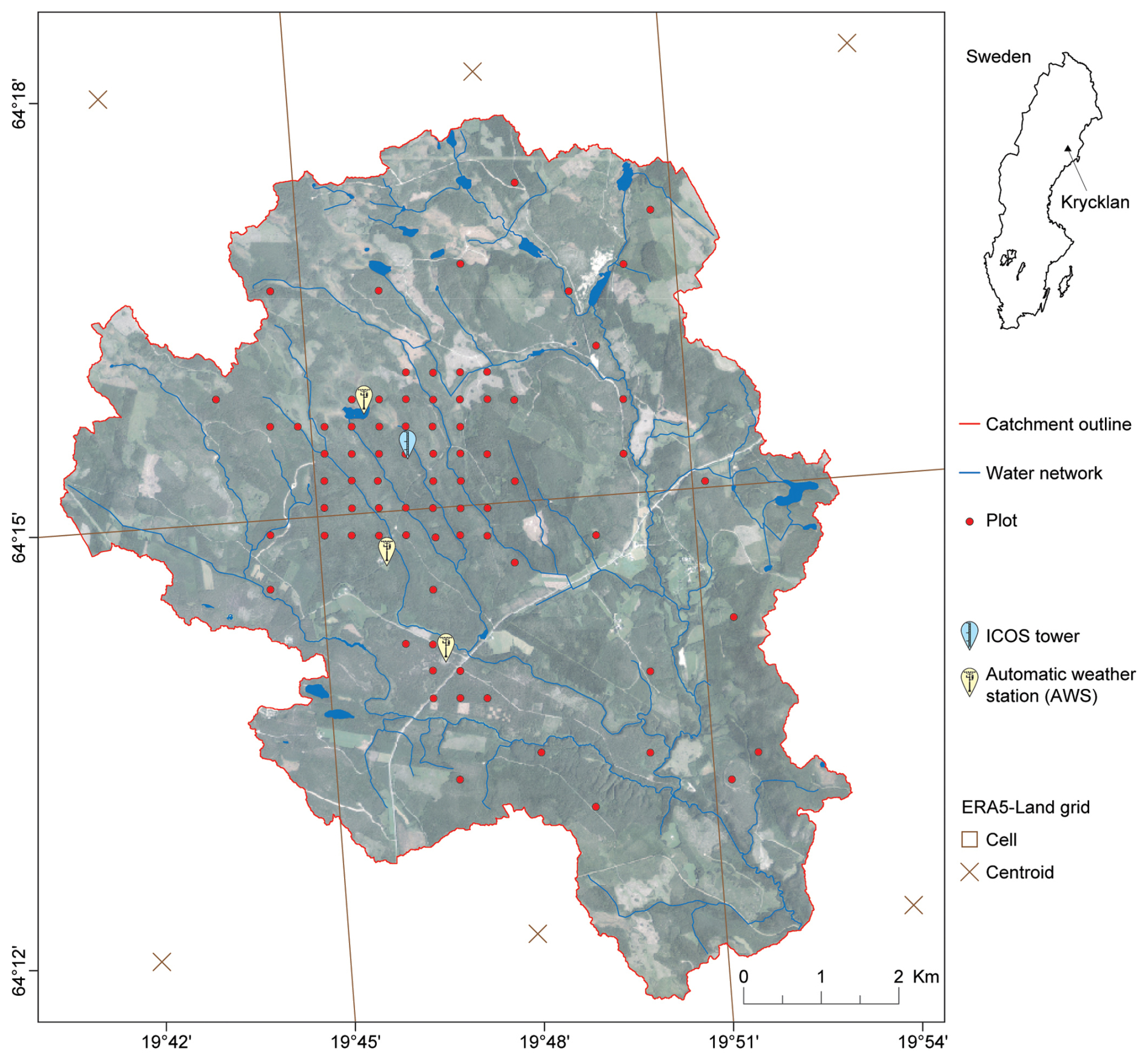
Figure 1 Overview of the Krycklan catchment showing the locations of the 78 soil moisture monitoring plots, the three automatic weather stations, and the ICOS tower, with the ERA5-Land grid superimposed. Orthophoto and water network: Lantmäteriet (2021).

2.2 Meteorological and environmental data

The extensive field inventory for the Krycklan catchment, combined with remote sensing and modeled data (e.g., from spatial interpolation and data assimilation), enabled us to evaluate a wide range of meteorological and environmental variables as potential predictors of soil moisture, the response variable in our study. We classified predictors into two groups: “spatial” predictors, which were assumed to be temporally static during the study season but varied spatially and were used to explain the spatial variability in soil moisture (Table 1), and “temporal” predictors, which varied temporally but not spatially across the study area and were used to explain the temporal variability in soil moisture (Table 2).

Table 1 All predictors of soil moisture spatial variability evaluated in this study. The 48 predictors are subdivided into four groups and 18 color-coded categories, listed in alphabetical order within each group and category based on the abbreviation code (“Abbr.” column). The table also displays the data source (field, non-field raster (N-field r), non-field vector (N-field v)), data type (qualitative (Ql) vs. quantitative (Qn)), and references. Each class of the qualitative variables is considered to be a distinct predictor in the analysis. The number of layers of the topographic and vegetation indices is reported in parenthesis after the predictor name, and it depends on the following: ¹ the spatial resolutions (0.5, 1, 2, 4, 8, 16, 32, and 64 m for the topographic indices and 0.4, 2, and 30 m for NDVI), ² the stream initiation thresholds (1, 2, 4, 8, 16, and 32 ha for depth to water and elevation above stream), and ³ the vertical distances (2 and 4 m for the downslope index). An asterisk denotes the 22 most relevant soil moisture predictors, which are displayed in Fig. 3. The 26 remaining predictors (without an asterisk) are shown in Fig. S2. The Supplement provides a detailed description of each variable listed in this table.

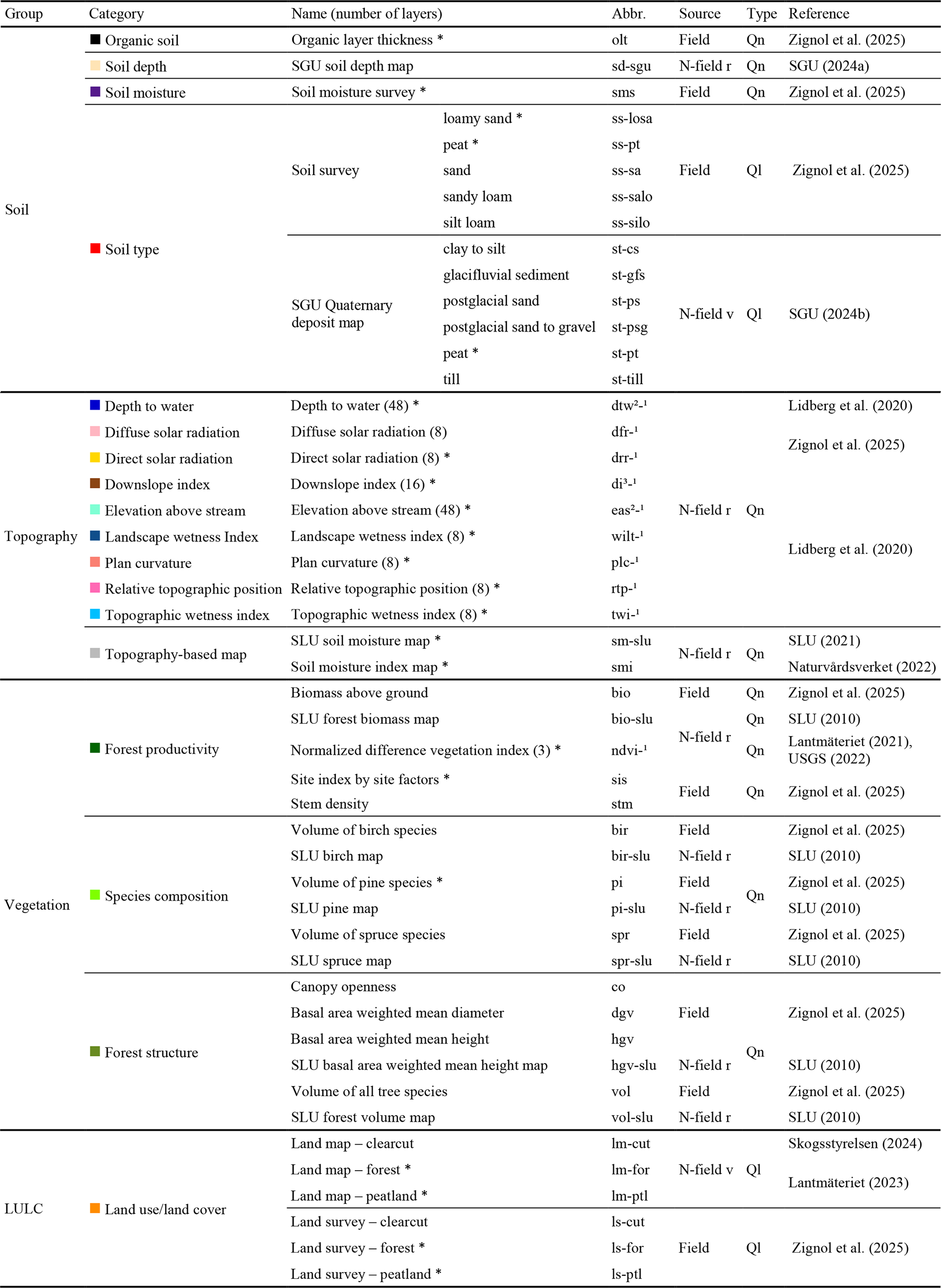
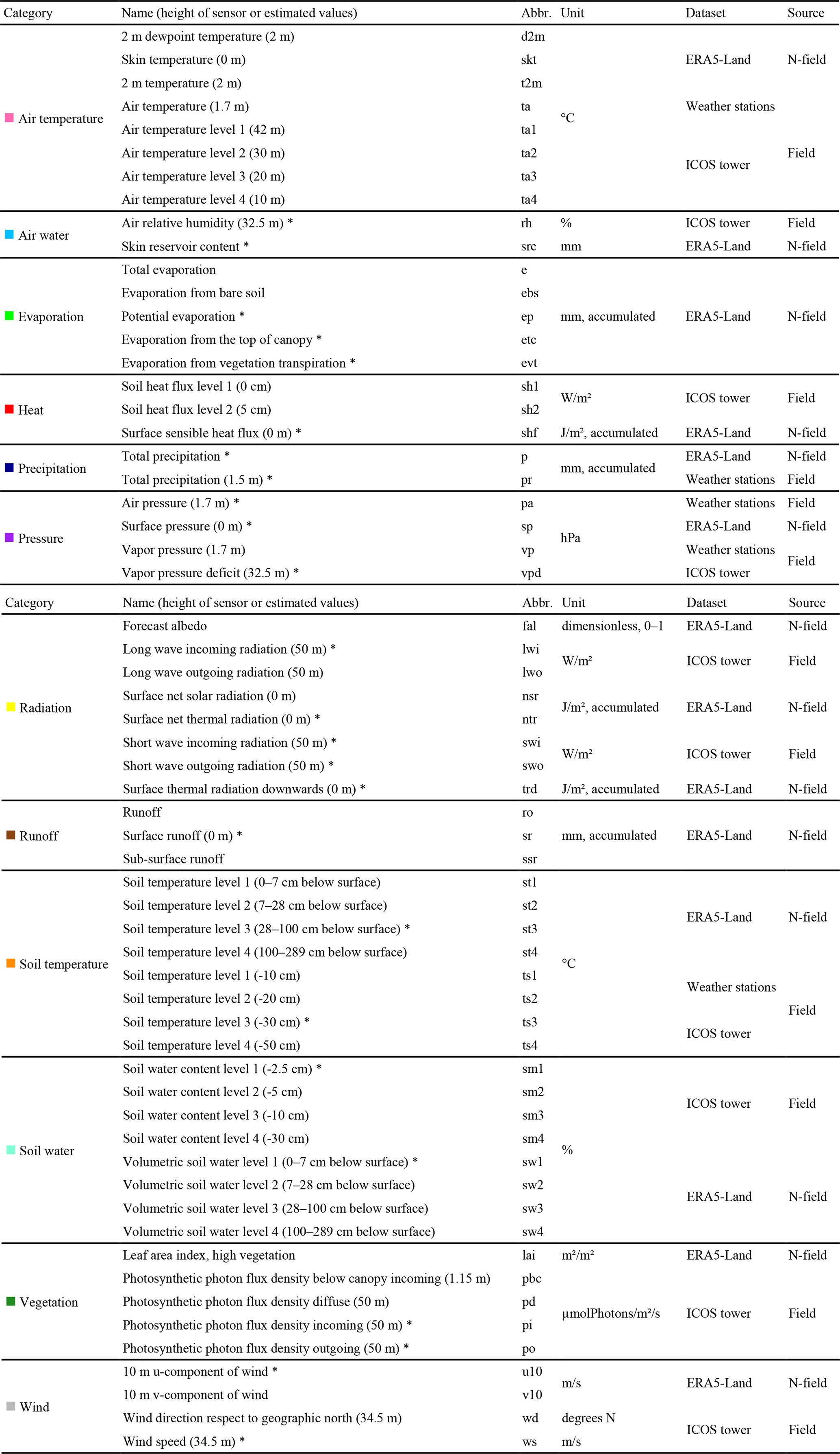
Table 2 All predictors of soil moisture temporal variability assessed in this study. The 60 predictors are subdivided into 12 color-coded categories, listed in alphabetical order within each category based on the abbreviation code (“Abbr.” column). The table also indicates the unit of measurement, the dataset (ERA5-Land, ICOS tower, or weather stations), and data source (field vs. non-field (N-field)). Whenever possible, either the sensor height (field data) or the height of the estimated values (ERA5-Land) is reported in parenthesis after the predictor name. An asterisk denotes the 25 most relevant predictors, which are displayed in Fig. 4. The 35 remaining predictors (without an asterisk) are shown in Fig. S3. The Supplement provides a detailed description of each variable listed in this table.

2.2.1 Response variable: soil moisture

To measure soil moisture, we selected a subset of 78 plots (Fig. 1) from a forest survey grid established in 2014 (Larson et al., 2023). This grid consists of 500 equally spaced plots (350 m apart), each of 10 m radius, covering the entire Krycklan catchment. Plot selection was informed by previous research (Larson et al., 2022), which classified most of the 500 plots into five soil moisture classes based on the Swedish National Forest Inventory (NFI) protocol. Our aim was to capture the full range and distribution of soil moisture conditions – from dry ridges to wet peatlands – observed across the Swedish forest landscape (see Fig. 3 in Ågren et al., 2021). To achieve this, approximately half of the selected plots were located in the central part of the catchment (Fig. 1), characterized by a highly heterogeneous landscape with diverse soil moisture conditions (Fig. S1). The remaining loggers were distributed throughout the catchment to ensure adequate spatial coverage while maintaining accessibility.

At each site, we measured the soil moisture content of the upper 14 cm of soil at a 15 min resolution using a TOMST temperature–moisture sensor (TMS) (Wild et al., 2019). We installed the loggers in June/July 2022 and we downloaded the data in October 2022, covering 92 d for all sites (from 5 July to 4 October). Because the sensor in the TMS logger relies on the time domain transmission method (Wild et al., 2019), we converted the raw signals into volumetric water content using the universal calibration equation presented in Kopecký et al. (2021). We also evaluated the soil-specific conversion functions proposed by Wild et al. (2019), but we found that some of the resulting volumetric water content values were nonsensical (e.g., < 0 % and > 100 %), particularly in mires. Consistent with findings from other studies in similar landscapes (e.g., Kemppinen et al., 2023), we concluded that these conversion functions were unsuitable for the soil types in Krycklan, specifically peat soils. Because the conversion did not alter the relative order among sites, we eventually adopted the universal curve for all plots, which produced a more realistic range of volumetric water content values.

We plotted each individual time series and conducted a thorough visual inspection to identify any anomalies. We checked for sudden drops in soil moisture that quickly reversed, as these often indicate potential loss of contact between sensor and soil. We carefully removed potentially erroneous data to ensure the reliability of our dataset. From the 15 min time series of volumetric water content, we calculated the mean daily time series for each plot, which served as the response variables in study aim (iii) (Table 3). We then aggregated these data to generate two additional datasets: the seasonal average of mean daily values for each plot and the spatially averaged mean daily time series across all sites, used as the response variables in study aims (i) and (ii), respectively (Table 3). For simplicity, when referring to our analysis, we use the term “soil moisture” in lieu of “volumetric water content at a depth of 0–14 cm”.

2.2.2 Spatial predictors: soil, topography, vegetation, and land use/land cover

In addition to monitoring soil moisture, we collected a vast array of environmental variables for each of the 78 plots (Fig. 1 and Table 1). Field variables were selected from the Krycklan inventory or during our field campaigns, whereas non-field variables were extracted from existing vector and raster maps, lidar-derived topographic indices, and other remote sensing products. In the case of topographic indices and the normalized difference vegetation index (NDVI), we extracted plot values from layers at different spatial resolutions (0.5, 1, 2, 4, 8, 16, 32, and 64 m for the topographic indices and 0.4, 2, and 30 m for NDVI) to assess how varying spatial resolutions explained soil moisture spatial variability. We also tested the effect of different user-defined thresholds, specifically two vertical distances (2 and 4 m) for the downslope index and six stream initiation thresholds (1, 2, 4, 8, 16, and 32 ha) for depth to water and elevation above stream. To facilitate the visualization and interpretation of the results, all predictors were subdivided into four groups, namely soil, topography, vegetation, and land use/land cover (LULC), and 18 color-coded categories (Table 1). Categories encompass analogous variables from distinct sources (e.g., land cover), diverse measures of a common feature (e.g., forest structure), the same variable at different spatial resolutions and/or user-defined thresholds (e.g., depth to water), or a combination of these cases. Note that classes of qualitative variables were treated as independent predictors in this analysis (e.g., soil survey). Table 1 lists all the spatial predictors evaluated in this study. A detailed description of each can be found in the Supplement.

2.2.3 Temporal predictors: meteorological forcings

For the temporal analysis, we selected meteorological variables (Table 2) from three datasets, including reanalysis data from the land component of the European Centre for Medium-Range Weather Forecasts (ECMWF) Atmospheric Reanalysis Fifth Generation (ERA5-Land) (Muñoz-Sabater, 2019; Muñoz-Sabater et al., 2021), atmospheric data from the ICOS tower (Peichl et al., 2024), and three automatic weather stations (Svartberget Research Station, 2022a, b, c). For each variable, we generated a single daily time series from 5 July to 4 October 2022 for the entire catchment by calculating the spatial average between either the three weather stations or the six ERA5-Land cells covering the Krycklan area (Fig. 1). To evaluate how varying temporal scales explained temporal variability of soil moisture, we created seven additional time series for each variable based on different temporal scales, including the preceding day and the average between the 3, 5, 7, 10, 14, and 21 preceding days. All predictors were subdivided into 12 color-coded categories to facilitate the visualization of the results. These categories group together analogous variables from distinct sources (e.g., precipitation), any variable measured at different depths (e.g., soil water) or heights (air temperature), diverse aspects of the same process (e.g., evaporation), or a combination of these cases. Table 1 lists all the temporal predictors analyzed in this study, with a detailed description of each provided in the Supplement.

2.3 Statistical model

To identify significant predictors of soil moisture, we used orthogonal projections to latent structures (OPLS) analysis, an enhanced version of partial least-squares regression (PLS) (Eriksson et al., 2013). OPLS separates the systematic variation in the predictors (X) into two parts: a predictive component (horizontal axis) that is directly associated with the response variable of interest (Y) and an orthogonal component (vertical axis) that represents the variation unrelated to Y. This method improves interpretability over ordinary PLS as it allows for identifying key variables for predicting Y while isolating less important variables that contain noise. OPLS is particularly well suited for high-dimensional datasets, as it effectively handles multicollinearity among predictors and reduces the risk of overfitting. In this two-dimensional space, positive or negative loadings on the predictive axis denote variables that are positively or negatively correlated with Y, with stronger correlations as distance from the origin increases. Conversely, loadings on the orthogonal axis, farther from the origin, indicate less correlated variables (i.e., higher noise). In our study, we used soil moisture measurements from dataloggers as the response variable (Y).

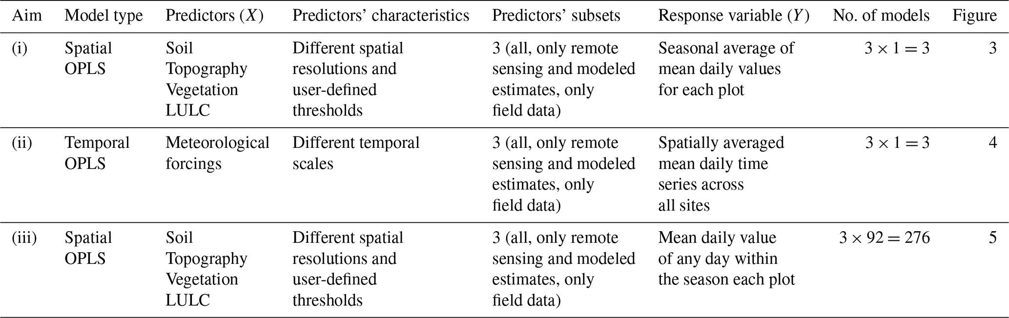
We created two types of OPLS models (Table 3). The first type, termed “spatial” OPLS, assessed the role of environmental predictors (soil, topography, vegetation, and LULC) (Table 1) in explaining the observed spatial distribution in soil moisture through direct plot-by-plot comparison. In these models, all environmental predictors varied across Krycklan but were assumed to be constant over time. Similarly, the response variable was spatially heterogeneous, but only one time step was included in each model. Specifically, to evaluate the relative importance of environmental predictors (aim i), we considered the soil moisture seasonal average, whereas to assess how the contribution of these predictors changed over time (aim iii), we ran the OPLS model 92 times using soil moisture daily values as the response variable (Table 3). The second type, termed “temporal” OPLS, evaluated the influence of meteorological predictors (Table 2) on the observed daily variations in soil moisture through direct day-by-day comparison (aim ii). In this model, all meteorological predictors and the response variable changed daily but were considered uniform across the study area (i.e., we calculated the spatial average) (Table 3).

To evaluate the predictive performance of field versus non-field data (aim iv), we ran both the spatial and temporal OPLS models using three different subsets of predictors: (1) only remote sensing and modeled estimates, including gridded and vector datasets such as topographic and vegetation indices and metrics, soil and LULC vector maps, and ERA5-Land time series; (2) only field measurements from surveys or permanent stations (i.e., weather stations and ICOS tower); and (3) a combination of all predictors. To assess the predictive performance of the overall OPLS models, we considered R² Y(cum), which represents the cumulative variation in the response variable (i.e., soil moisture) explained by the three subsets of predictors.

To estimate the predictive performance of each variable, we also calculated the variable importance on projection for the predictive component (VIP_predictive) for the 94 OPLS models based on all predictors (Table 3). These values are normalized such that if each X variable contributed equally to the model, their VIP_predictive would be 1. Variables with a VIP_predictive value greater than 1 are considered relevant predictors, with higher scores indicating greater predictive power (Eriksson et al., 2013). We used this metric and threshold to distinguish relevant soil moisture predictors, presented in Figs. 3 and 4, from less important ones, included in the Supplement (Figs. S2 and S3). We processed all the data in R version 4.3.0 (R Core Team, 2023), we generated all OPLS models and calculated the related VIP_predictive scores in SIMCA 17.0, and we drew all the figures using the R ggplot2 package (Wickham, 2016), ArcGIS Pro (Esri Inc., 2023), and Adobe Illustrator (Adobe Inc., 2024).

Table 3 All OPLS models developed in this study.

3 Results

3.1 Observed spatial and temporal variability in soil moisture

Analysis of the logger data revealed large spatial variability in both seasonal averages and seasonal standard deviations of soil moisture, ranging from 14 % to 56 % (∼60 % = fully saturated) and 0.4 % to 5.6 %, respectively (Fig. 2a). Among the 78 sites studied, 14 exhibited an increasing trend in soil moisture over the season, seven a decreasing trend, and the remaining 57 no trend, based on the nonparametric Mann–Kendall test (Mann, 1945; Kendall, 1975) at 95 % confidence level (Fig. 2bc). The magnitude of soil moisture change over the entire study period, indicated by the trend Theil–Sen slope (Sen, 1968), varied between −8.4 % and 10 % (Fig. 2b, Table S1 in the Supplement), whereas the strength of the monotonic association between soil moisture and time, as measured by Kendall's correlation coefficient (τ), ranged from −0.58 to +0.57 (Table S1). Daily peaks in soil moisture were typically associated with major precipitation events, although the magnitude of these peaks and subsequent declines during dry periods varied considerably across locations (Fig. 2c). Conversely, the daily spatial variability (i.e., standard deviation) in soil moisture (black line) exhibited a sharp decline during precipitation events (especially in August and September), followed by a steady increase leading up to peaks at the culmination of subsequent dry periods (bottom part of Fig. 2c). The soil moisture time series from ERA5-Land (brown lines) closely tracked the temporal variability of the mean across all sites (red line) but underestimated daily soil moisture amounts averaged across all sites (Fig. 2c). Overall, Fig. 2 shows that the 78 sites responded differently to similar weather conditions and that the spatial variability in soil moisture among all sites is much larger than the temporal variability in soil moisture observed throughout the study season.

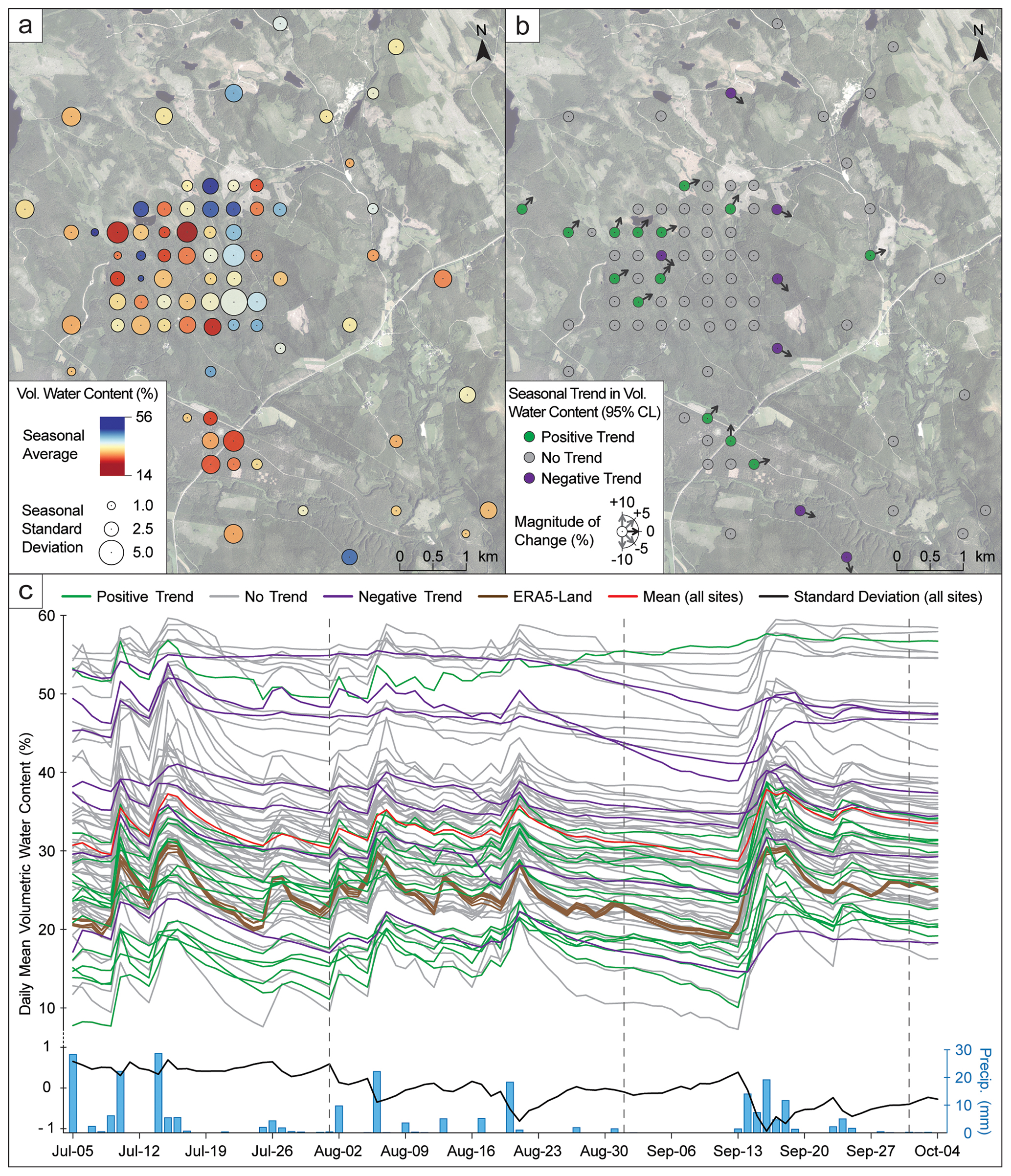
Figure 2 Spatial and temporal variation of daily mean soil moisture (i.e., volumetric water content) measured by 78 loggers across the Krycklan catchment from 5 July to 4 October 2022. Panel (a) displays the seasonal average and standard deviation of the measurements. Panel (b) shows seasonal trends identified using the Mann–Kendall test at a 95 % confidence interval. Panel (c) presents the time series plot, with logger data grouped by color according to trend type. The graphic includes additional data for comparison: estimates from six ERA5-Land cells covering the catchment (brown lines), spatial mean (red line) and standard deviation (black line) among sites, and mean precipitation across Krycklan derived from weather stations (bottom bar plot). For clarity, refer to Fig. 1 for the locations of the ERA5-Land cells and weather stations. Orthophoto in panels (a) and (b): Lantmäteriet (2021).

3.2 Controls on soil moisture variability

OPLS plots served as a means to visualize in two dimensions the relative importance of factors controlling soil moisture variability, with loadings located closer to the horizontal axis (i.e., lower noise) and farther from the vertical axis (i.e., higher predictive power) indicating the most relevant predictors. Variables on the right side of the plot are positively correlated to soil moisture, while those on the left side are negatively correlated. Remote sensing and modeled estimates are represented by circles (raster datasets) or rhombuses (vector datasets), whereas field measurements are displayed as triangles. The size of the symbols is proportional to either the spatial resolution or the temporal scale of the potential soil moisture predictors. Variables are grouped together into color-coded categories to facilitate the reading of the OPLS plots. When multiple spatial resolutions or temporal scales were investigated for a certain variable, its loadings were connected through guides transitioning from high to low resolution or scale, and only the optimal resolution or scale was labeled. The upcoming two sections will focus on outlining the key features of the spatial OPLS plot (Figs. 3 and S2) and the temporal OPLS plot (Figs. 4 and S3), respectively. Due to the large number of variables analyzed in this study, Figs. 3 and 4 only present the most relevant predictors (VIP_predictive greater than 1, marked by an asterisk in Tables 1 and 2), whereas all remaining variables are included in the Supplement (Figs. S2 and S3).

3.2.1 Spatial variation

Relative topographic position emerged as the strongest predictor of soil moisture at a 16 m resolution (rtp-16), but its predictive performance decreased at lower and higher resolutions (Fig. 3). Similar to relative topographic position, depth to water and elevation above stream were negatively correlated with soil moisture, with loadings clustered in the bottom-left quadrant (Figs. 3 and S2). These two indices showed reduced performance and increased noise for higher stream initiation thresholds (Fig. S2). However, while coarse resolution (64 m) was optimal for elevation above stream, high resolution (0.5 or 1 m) was preferable for depth to water (Fig. S2), with eas1-64 and dtw1-05 overall performing best (Fig. 3). In the top-right quadrant (i.e., positively correlated), the topographic wetness index and landscape wetness index were good predictors of soil moisture at their optimal resolutions of 32 m (twi-32) and 4 m (wilt-4), respectively (Fig. 3). At these resolutions, they performed comparably to the soil moisture index map (smi) and the SLU soil moisture map (sm-slu), with the last one exhibiting slightly higher performance (Fig. 3). The downslope index and plan curvature at their optimal vertical distance and/or spatial resolution (di2-32 and plc-32), also positively correlated with soil moisture, showed slightly lower predictive power but introduced less noise (loadings closer to the origin) (Fig. 3). Direct solar radiation was only relevant at a coarse resolution (drr-64) (Fig. 3), while diffuse solar radiation was a less important predictor (Fig. S2).

As for soil, three field variables – peat soil class (ss-pt), soil moisture classes (sms), and organic layer thickness (olt) – were robust predictors, showing a positive correlation with soil moisture and low noise (Fig. 3). The peat class from the SGU soil type map (st-pt) was also positively correlated, yet it explained less variability than the analogous field predictor (i.e., ss-pt). Both peatland (positively correlated) and forest (negatively correlated) LULC classes similarly revealed that the data collected in the field (ls-ptl and ls-for, respectively) provided slightly better results than using information from an existing map (lm-ptl and lm-for, respectively). Finally, the loamy sand class from the soil survey (ss-losa) was, to a lesser extent, an important predictor, negatively correlated with soil moisture. The remaining soil and LULC variables, whether derived from field observations or existing maps, performed poorly in predicting soil moisture (Fig. S2).

Among the vegetation-related variables, volume of pine (pi) showed the highest predictive performance, followed by the normalized difference vegetation index at 2 m resolution (ndvi-2) and the site index by site factors (sis), with pi and sis being negatively correlated with soil moisture, whereas ndvi-2 was positively correlated (Fig. 3). While ndvi-2 and pi slightly outperformed, in terms of predictive power, analogous predictors at coarser spatial resolutions (ndvi-30 and pi-slu, respectively), they also introduced more noise (Figs. 3 and S2). The remaining vegetation variables exhibited low predictive performance or high noise, which made them less suitable as soil moisture predictors (Fig. S2).

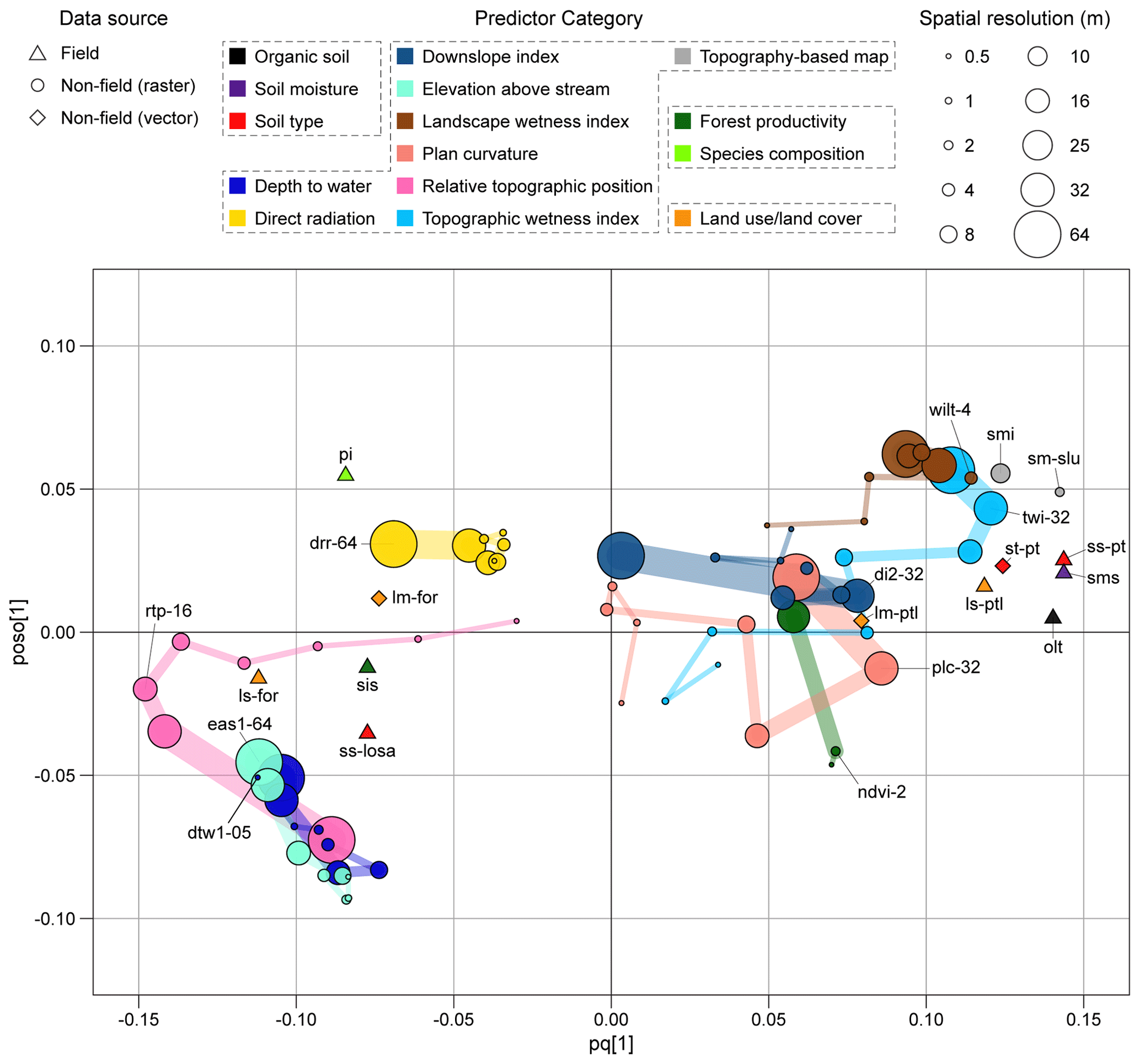
Figure 3 OPLS loading plot showing the relationship between a large array of “spatial” predictors, which vary spatially but remain constant over time, and the mean seasonal soil moisture (5 July–4 October 2022). Both the spatial predictors (X variables) and the response variable (Y variable) were gathered for 78 sites across the Krycklan catchment (Fig. 1 for the site locations). The spatial predictors, overall describing soil, topography, vegetation, and land use/land cover at each site (gray dotted boxes in the figure legend), were either directly measured in situ (symbolized by triangles) or estimated through remote sensing or modeling techniques (depicted as circles or rhombuses depending on the dataset format). These predictors were organized into 18 color-coded categories (see Table 1; here only 15 are shown) to enhance plot readability. Gridded (i.e., raster) predictors are characterized by a certain spatial resolution (expressed in meters, representing the length of the grid cell side), which is proportional to the size of the circles. To visualize the effects of spatial resolution, guides connect loadings of the same variable moving from high to low resolutions, with the variable name visible only in correspondence to the optimal resolution (refer to Table 1 for variable labels). High positive and negative loadings on the predictive axis (pq[1]) represent variables that are positively and negatively correlated with the response variable (Y), with stronger correlation further away from the origin. The orthogonal axis (poso[1]) indicates how much of the variation for each variable was not correlated with the response variable (Y). This figure only shows the 22 most relevant predictors (VIP_predictive greater than 1, marked by an asterisk in Table 1). If multiple user-defined thresholds were tested for a certain topographic index (i.e., depth to water, downslope index, and elevation above stream), the plot displays only the best-performing one. All 26 remaining variables are included in Fig. S2.

3.2.2 Temporal variation

Soil moisture estimates from ERA5-Land and ICOS measurements were understandably the two best predictors of the spatially averaged time series of soil moisture recorded at the 78 study plots (Fig. 4). Their predictive performance was highest when selecting the top soil layer and matching the temporal scale with the response variable (sw1-0 and sm1-0). Most loadings of these two predictors were positively correlated with the response variable (Y), though the strength of the correlation generally decreased and noise increased with longer temporal scales and deeper soil layers (Fig. S3).

The temporal OPLS analysis revealed that the optimal temporal scale for most predictors ranged between 5 and 7 d preceding the datalogger recordings, with predictive performance decreasing for both shorter and longer temporal scales (Fig. 4). Skin reservoir content, which accounts for the water in the vegetation canopy and in a thin layer on top of the soil, at the 7 d scale (src-7), emerged as a strong predictor, positively correlated with soil moisture and associated with minimal noise. Surface air pressure at the 7 d scale (sp-7 and pa-7) was also a robust predictor, showing an inverse correlation with soil moisture. Evaporation from the top of the canopy at the 5 d scale (etc-5) is in the vicinity yet towards higher noise and lower predictive values.

The remaining variables explaining the temporal variability in soil moisture clustered into three distinct areas (Fig. 4). On the right side of the OPLS plot, therefore indicating a positive relationship with soil moisture, two clusters stood out: air relative humidity (rh-7), surface net thermal radiation (ntr-7), surface sensible heat flux (shf-3), evaporation from vegetation transpiration (evt-7), and potential evaporation (ep-5) in the top quadrant and precipitation (pr-7 and p-5), surface runoff (sr-5), longwave (i.e., thermal) incoming radiation (lwi-5 and trd-5), and wind speed (ws-5) in the bottom quadrant. The third cluster, located in the bottom-left quadrant, consisted of predictors negatively correlated with soil moisture, including incoming and outgoing shortwave radiation (swo-5 and swi-5), incoming and outgoing photosynthetic photon flux density (po-5 and pi-5), vapor pressure deficit (vpd-7), 10 m u component of wind (u10-5), and soil temperature (ts3-21 and st3-21). All air temperature variables, along with other less relevant predictors of soil moisture, are shown in the Supplement (Fig. S3).

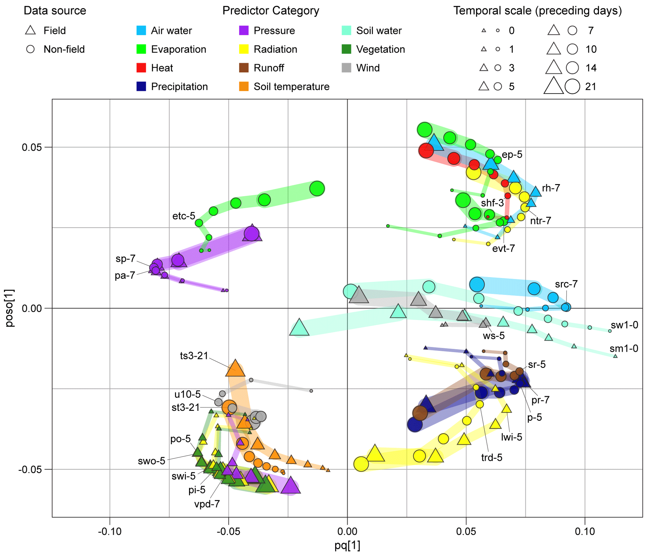
Figure 4 OPLS loading plot illustrating the relationship between a large array of “temporal” predictors, which do not vary spatially but change over time, and daily mean soil moisture (i.e., volumetric water content) averaged across 78 sites within the Krycklan catchment (refer to Fig. 1 for the site locations). Both the temporal predictors (X variables) and the response variable (Y variable) were aggregated at the daily temporal scale from 5 July to 4 October 2022. The temporal predictors were either directly measured at the ICOS tower or at weather stations within Krycklan (symbolized by triangles) or extracted from the ERA5-Land dataset (depicted as circles). These predictors were organized into 12 color-coded categories (see Table 2; here only 11 are shown) to enhance plot readability. All predictors are characterized by a certain temporal scale, represented by the size of the triangles or circles. To visualize the effects of temporal scale, guides connect loadings of the same variable moving from high to low scales, with the variable name visible only in correspondence to the optimal scale (refer to Table 2 for variable labels). High positive and negative loadings on the predictive axis (pq[1]) represent variables that are positively and negatively correlated with the response variable (Y), with stronger correlation further away from the origin. The orthogonal axis (poso[1]) indicates how much of the variation for each variable was not correlated with the response variable (Y). This figure only shows the 25 most relevant predictors (VIP_predictive greater than 1, marked by an asterisk in Table 2), but the 35 remaining predictors are included in Fig. S3.

3.3 Spatial soil moisture variability under different wetness conditions

The relative importance of predictors in influencing spatial soil moisture variability remained relatively consistent over the study period in the Krycklan catchment, with their VIP_predictive values showing little variation throughout the season (Figs. 5 and S4). The SLU soil moisture map (sm-slu) exhibited the smallest variation among all predictors (seasonal standard deviation of VIP_predictive: 0.03) (Fig. 5). In contrast, two vegetation-related variables and direct solar radiation (ndvi-2, pi, and ddr-64) showed the largest variation (seasonal standard deviation of VIP_predictive: 0.09), reflecting generally better performances in the first half of the season (especially at the transition from July to August) compared to the second half (Fig. 5).

Most predictors experienced abrupt drops in VIP_predictive during intense and/or multi-day precipitation occurrences (e.g., 16 September) (Fig. 5), when the soil moisture variability across all 78 sites was also at its lowest (bottom graphic in Fig. 2c). However, some topographic indices (dtw1-05, eas1-64, and, to a lesser degree, plc-32 and rpt-16) showed increasing predictive power after the beginning of a precipitation event (e.g., July 15 or September 15) (Fig. 5). During drying periods (e.g., between late August and almost mid-September), the VIP_predictive values of the majority of predictors tended to steadily and slowly decrease, except for three notable exceptions: the loamy sand soil class (ss-losa), the site index by site factors (sis), and the downslope index (di2-32).

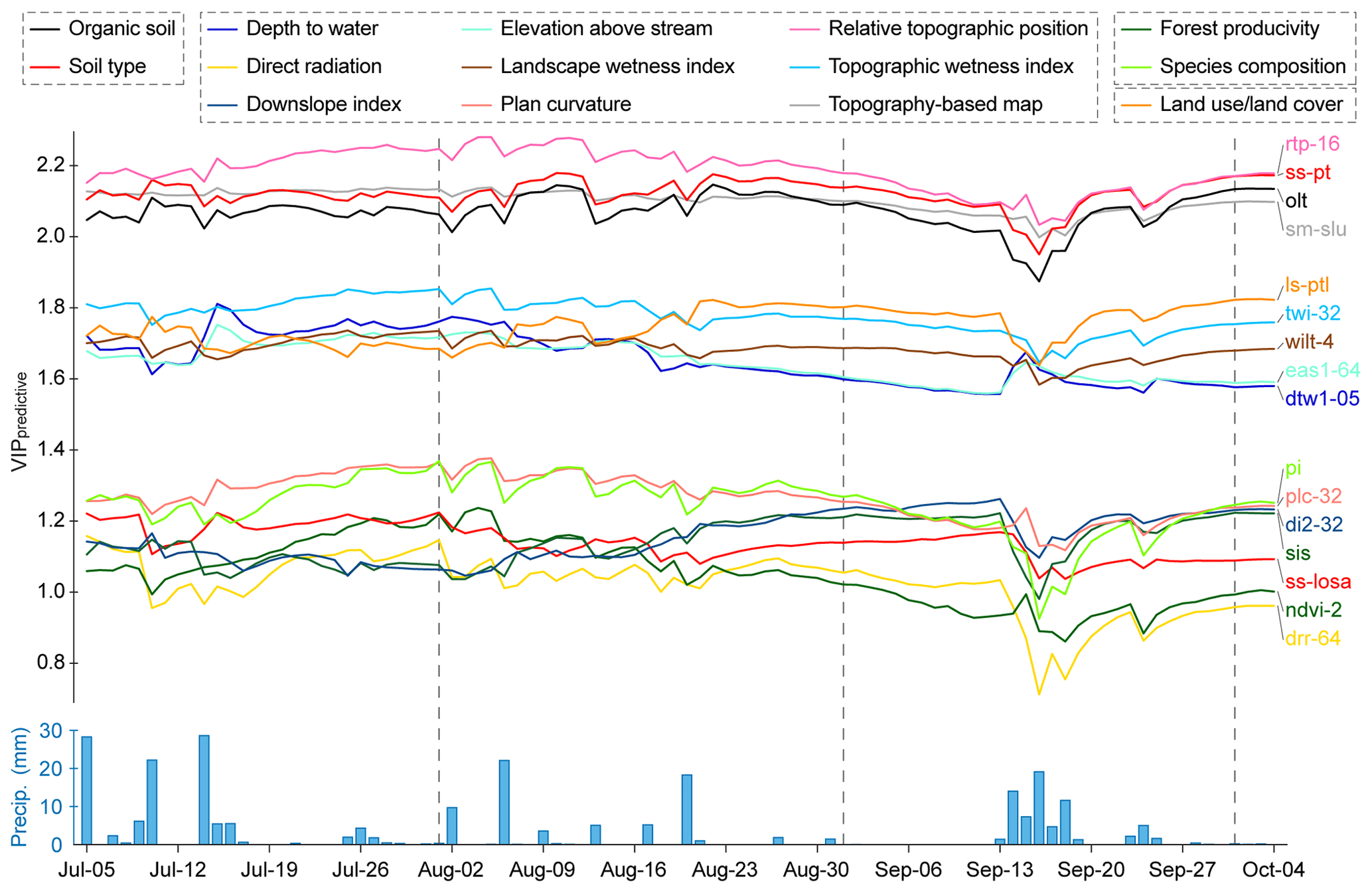
Figure 5 VIP_predictive values of 92 spatial OPLS models generated using mean daily soil moisture over the study season (5 July–4 October 2022) as the response variable (Y). The lower section of the figure displays the mean precipitation across Krycklan derived from weather stations (refer to Fig. 1 for their locations). The spatial predictors, overall describing soil, topography, vegetation, and land use/land cover at each site (gray dotted boxes in the figure legend), were organized into 18 color-coded categories (see Table 1; here only 14 are shown) to enhance plot readability. Color-coded labels on the right side of the figure are ordered according to their VIP_predictive on the last day of the study season (4 October 2022). To avoid clutter and highlight the key findings, only a subset of predictors is presented, but a graphic with all 22 relevant predictors (VIP_predictive greater than 1) displayed in Fig. 3 is included in Fig. S4.

3.4 Field measurements compared to remote sensing and modeled estimates

Field measurements generally outperformed remote sensing and modeled data by approximately 6 % in both spatial and temporal OPLS models, with the combination of all predictors yielding the highest performance (Fig. 6a). In the temporal OPLS models, more variance in soil moisture dynamics was explained by data from the ICOS tower and weather stations (R² Y(cum) = 0.96) compared to ERA5-Land estimates (R² Y(cum) = 0.90). A similar pattern emerged in the spatial OPLS models, where soil, vegetation, and LULC data collected in the field (R² Y(cum) = 0.51) better explained spatial variability in seasonal soil moisture than topographic indices and existing soil, vegetation, and LULC maps (R² Y(cum) = 0.45).

In the spatial OPLS daily models (Fig. 6b), these two subsets of predictors showed the same relative ranking, with field measurements (green line) outperforming remote sensing and modeled estimates (blue line) throughout the season. However, they responded differently to changing wetness conditions. This was most evident between late August and mid-September, a period marked by 24 nearly rain-free days followed by 5 d of persistent precipitation. R² Y(cum) of field-based models (green line) increased sharply during the dry spell, then abruptly dropped by 10 % with the onset of rain. In contrast, the models using remote sensing and modeled data showed only a marginal improvement during the dry period and a smaller and more gradual decline (∼2 %) during rainfall.

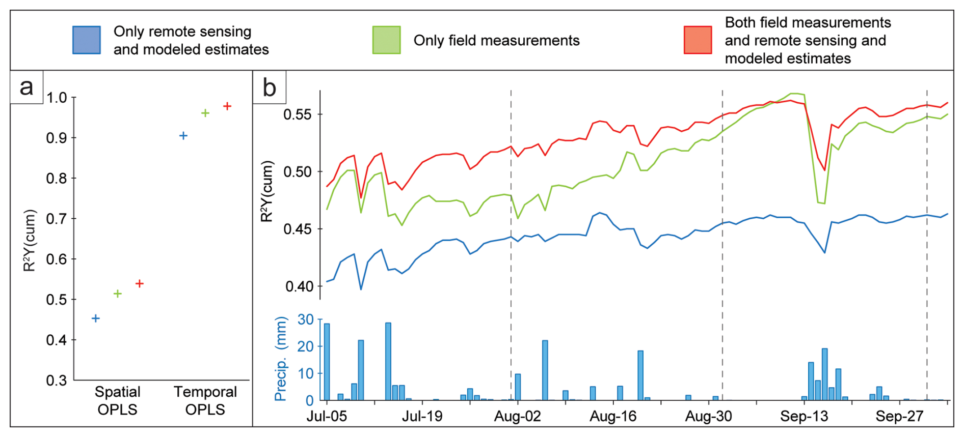
Figure 6 OPLS model performance using only remote sensing and modeled predictors (blue), only field predictors (green), and all predictors combined (red). R² Y(cum) indicates the cumulative proportion of variance in the response variable Y (i.e., soil moisture) explained by each model (see Table 3 for the models' specifications). Panel (a) shows the R² Y(cum) values, indicated by crosses, of models using either the seasonal average per plot (spatial OPLS) or the spatially averaged daily time series across all sites (temporal OPLS) as the response variable. Panel (b) displays the R² Y(cum) values of 92 daily spatial OPLS models over the study period (5 July–4 October 2022), with mean precipitation across Krycklan (from weather stations shown in Fig. 1) plotted below for reference.

4 Discussion

In this study, we investigated a vast array of climatic and environmental factors controlling the spatial patterns and temporal dynamics of surface soil moisture in a boreal forest landscape in northern Sweden with the purpose of providing new insights into modeling and mapping soil moisture. Specifically, we evaluated the ability of numerous variables extracted from multiple sources, including field measurements, remote sensing retrievals, and modeled data at different spatial resolutions and temporal scales, to explain soil moisture variations recorded during 3 snow-free months in 2022 by 78 dataloggers distributed across the Krycklan catchment. In the sections that follow, we discuss the primary findings from our analysis.

4.1 Spatial variation

We found that all four groups of spatial predictors considered in this analysis, namely topographical features, soil properties, vegetation characteristics, and land use/land cover (LULC), played a significant role in explaining spatial variations in soil moisture (Fig. 3). With the advent of lidar-derived DEMs at very high spatial resolution, researchers have increasingly used terrain indices, or a combination of them, as a proxy for soil moisture (Kemppinen et al., 2018; e.g., Kopecký et al., 2021; Riihimäki et al., 2021; Winzeler et al., 2022), including the 10 m resolution soil moisture index map (smi) (Naturvårdsverket, 2022) and the 2 m resolution SLU soil moisture map (sm-slu) (Ågren et al., 2021) that we evaluated in our study. While these maps correlated well with soil moisture measured in the field, our analysis revealed that soil predictors, such as organic layer thickness and soil texture, vegetation-related variables, and land cover information distinguishing between mire and forest were also important. The relevance of integrating soil and terrain information to characterize soil moisture patterns in the context of hydrological modeling was highlighted by similar studies at the catchment scale (e.g., Baldwin et al., 2017). Previous research has demonstrated that soil properties are determinant in controlling soil moisture spatial variance at the hillslope (Wang et al., 2023) and regional (Wu et al., 2020) scales as well. Consistent with other studies (e.g., Sørensen and Seibert, 2007; Ågren et al., 2014; Lidberg et al., 2020; Larson et al., 2022), our analysis also indicated that the performance of any terrain index varies greatly depending on the threshold and resolution considered, with a 1 ha stream initiation threshold providing the best results and 0.5 m spatial resolution being the optimal choice only in one case (i.e., depth to water index). Interestingly, relative topographic position at 16 m resolution (rtp-16) emerged as the best predictor of soil moisture spatial variability, capable of identifying wetter depressions and drier ridges in the landscape (Weiss, 2001). While several examples in the literature demonstrate the importance of this index in soil moisture estimation (e.g., Engstrom et al., 2005; Zhao et al., 2021), it is somewhat surprising that Larson et al. (2022), who used five soil moisture classes estimated in the field as the response variable (sms predictor in our study) (see Table 1 and Fig. 3), observed that relative topographic position was not among the best-performing variables in the Krycklan catchment. Therefore, in the pursuit of estimating spatial variability in soil moisture, we advise caution when selecting terrain indices and their spatial resolutions and thresholds. We argue that an enhanced spatial resolution in topographical data does not necessarily compensate for the absence of soil, vegetation, and LULC information. We finally reiterate the importance of soil moisture datalogger measurements to validate predictive models.

4.2 Temporal variation

Our research demonstrated that daily soil moisture fluctuations within the Krycklan catchment are strongly influenced by the hydrological and meteorological conditions over 5 to 7 d preceding soil moisture measurements, regardless of whether these conditions were estimated (ERA5-Land dataset) or measured directly in the field (weather stations and ICOS tower) (Fig. 4). Among other variables, increased soil moisture was correlated with lower air pressure, shortwave radiation, vapor pressure deficit, and evaporation from the top of the canopy; conversely, it was associated with higher thermal (longwave) radiation, precipitation, air humidity, evapotranspiration, and wind speed. Averaged conditions over 5 to 7 d for all these variables exhibited the strongest correlation with daily variations in soil moisture in Krycklan, indicating both lagged and cumulative effects of these processes on soil moisture. Previous research has also highlighted the importance of considering multi-day accumulations and time lags between meteorological drivers and soil moisture response (Williams et al., 2009; Pan, 2012; Li et al., 2024), with most studies focusing on the precipitation–soil moisture relationship. Parent et al. (2006) showed that the transfer of energy from precipitation to soil moisture via infiltration, percolation, and redistribution processes mostly occurs over temporal scales ranging between 2 and 14 d. Piao et al. (2009) proved that precipitation frequency can be a more crucial factor than precipitation amount in shaping soil moisture variations, making it essential to account for the cumulative effect of precipitation over multi-day temporal scales (Ge et al., 2022). Our study identified soil temperature (28–100 cm below the surface) as the most notable exception to the optimal temporal scale of 5 to 7 d observed for almost all other relevant predictors. While we found a negative correlation between soil temperature and soil moisture as expected (Aalto et al., 2013), the strongest effects emerged at the 3-week scale (the longest temporal scale considered in our analysis), possibly because soil temperature at those depths (28–100 cm) also varies more slowly compared to topsoil temperature. Soil temperature, along with air temperature – which showed weak correlation with soil moisture in our study – might better correlate with soil moisture over longer temporal scales, such as seasonal or annual (Liang et al., 2024). In regard to our findings, it is important to acknowledge that the optimal temporal scale for estimating daily fluctuations in soil moisture can vary according to soil drainage conditions (Parent et al., 2006) and initial wetness conditions characterizing specific climate zones (Chai et al., 2020) or resulting from different seasonal and annual variations in large-scale climate patterns (Li et al., 2024).

4.3 Temporal stability of soil moisture patterns

Different initial wetness conditions can also influence the processes controlling spatial variability in soil moisture (Famiglietti et al., 1998; Western et al., 2004; Joshi and Mohanty, 2010; Mei et al., 2018; Gao et al., 2020; Wang et al., 2023). Although the ranking among predictors remained nearly constant over the study season, we observed that their predictive power changed nonuniformly in relation to daily fluctuations in wetness conditions (i.e., variables responded differently to the same wetness conditions in any day) (Fig. 5). Previous studies have indicated that, under drying conditions, lateral water movement is gradually replaced by vertical water movement (Grayson et al., 1997; Western et al., 1999; Rosenbaum et al., 2012), and the spatial variability in soil moisture is likely due to diverse infiltration and evapotranspiration rates related to the spatial distribution of soil and vegetation features (Teuling and Troch, 2005; Takagi and Lin, 2012; Jia et al., 2013; Launiainen et al., 2019). Conversely, the soil moisture spatial variability under rewetting conditions is mostly determined by topographical structures that guide lateral subsurface flow and surface runoff (Grayson et al., 1997; Gaur and Mohanty, 2013). These findings are in line with the results of our study, suggesting that higher infiltration rates in loamy sand soils compared to other soil types and diverse evapotranspiration rates associated with different vegetation (i.e., different site index values) increasingly contributed to the observed spatial distribution of soil moisture, particularly during drying periods (e.g., late August to mid-September in our case), while most topographic variables became steadily less relevant during this time. On the other hand, during large precipitation events, topographic indices showed an initial drop in the predictive power, likely due to the accumulation of water in the top soil layer and the consequent reduced spatial variability in soil moisture among sites, followed by a time-lagged peak in the predictive power, likely associated with the beginning of lateral subsurface flow driven by topographical features (Grabs et al., 2012). Regarding vegetation, we also observed a clear seasonal pattern: during the peak of the growing season, generally characterized by warmer and longer days, the spatial heterogeneity of vegetation usually had a larger effect on soil moisture distribution. This may be due to stronger effects of increased transpiration or shading during this period, leading to more pronounced differences across plots, whereas this influence diminished towards the end of the summer, when days were usually cooler and shorter. Seasonal patterns in solar radiation affected evapotranspiration rates and soil moisture levels differently not only in forests compared to peatlands, with forests responding more strongly due to higher canopy cover and biomass (Mackay et al., 2007), but also depending on tree species composition, with pine being potentially more responsive to high radiation than spruce (Lagergren and Lindroth, 2002). These findings reiterate the importance of considering the temporal stability of spatial soil moisture patterns under changing wetness conditions (Wang et al., 2023), and we suggest that future research should focus on modeling soil moisture dynamics over longer timescales, beyond a single growing season, particularly in high-latitude environments, where this remains an underexplored topic.

4.4 Mapping spatiotemporal variability in soil moisture

While extensive literature exists assessing the accuracy of remote sensing and modeled estimates of soil moisture based on analogous data measured in situ (Romano, 2014; Petropoulos et al., 2015; Dorigo et al., 2021), we are not aware of any study explicitly comparing the ability of numerous field versus non-field environmental and climate predictors in explaining spatial and temporal variations in soil moisture. Field measurements generally outperformed remote sensing and modeled data in terms of both overall model performance (Fig. 6) and when comparing pairs of analogous variables from different sources, especially in the case of spatial variability (Figs. 4 and S2). However, field data alone, which included soil, vegetation, and LULC information, did not yield the highest performance, as DEM-derived topographic information also proved essential, with both types of predictors influencing soil moisture differently depending on prevailing weather conditions (Figs. 5 and 6). We also acknowledge that, even when combining both field and non-field environmental variables in our models, the spatial distribution of soil moisture was not fully captured. In part, this may be explained by temporal discrepancies in data collection, with some data obtained prior to the 2022 study season (see the Supplement), and measurement inaccuracies, including errors in soil moisture datalogger recordings. In particular, calibrating TOMST sensors in organic-rich peat soils remains challenging, and volumetric water content measurements in these soils may not reflect full saturation (Menberu et al., 2021; Kemppinen et al., 2023). Moreover, we assumed spatial homogeneity for meteorological forcings across the Krycklan catchment, a reasonable assumption for variables like precipitation but less so for variables such as soil and air temperatures (Aalto et al., 2022; Kolstela et al., 2024), whose fine-scale variations likely influenced soil moisture patterns. At even finer spatial scales, variations in soil moisture may have stemmed from local factors not represented by our predictors, such as soil discontinuities, small understory vegetation, and the presence of stones (Parajuli et al., 2020). Future studies should focus on analyzing soil moisture datasets with higher temporal variability (e.g., covering the entire snow-free season, including post-snowmelt periods, and multiple seasons or years), evaluating more accurate lidar-derived vegetation metrics, accounting for microclimatic variations, and comparing catchments with diverse characteristics (e.g., spanning a large latitudinal gradient). For future soil moisture mapping, greater efforts should be devoted to improving the quality and resolution of spatially continuous soil information. The lack of detailed soil maps describing soil properties such as texture, structure, and organic matter content was most likely the major cause behind the relatively lower predictive performance of remote sensing and modeled data compared to field data. Enhanced soil maps would benefit not only data-driven approaches to soil moisture mapping but also physically based modeling efforts that rely on such inputs. Informed by the results of this study, we are now able to select a smaller subset of key spatial and temporal predictors of soil moisture, which, in the future, could be integrated into a machine learning model to generate dynamic soil moisture maps for Krycklan. While machine learning models can handle high-dimensional data, pre-selecting variables enhances interpretability, reduces overfitting, and ensures that inputs reflect the variation most relevant to soil moisture dynamics (Meyer et al., 2019). Due to their ability to process large volumes of data, such models can leverage detailed spatial and temporal information from multiple sources to potentially map soil moisture at both high spatial and temporal resolutions across vast geographic areas.

5 Conclusions

The Krycklan field infrastructure provided a unique setting for designing a comprehensive study to advance our understanding of the relationship between surface soil moisture and its controls in a forest boreal landscape. By combining remote sensing and modeled data with field measurements across 78 sites in the Krycklan catchment, this study is among the first to examine such a broad range of climatic and environmental factors at different spatial resolutions and temporal scales, focusing on both the spatial and temporal components of soil moisture variability. Our findings suggest that topographical features, soil properties, vegetation characteristics, land use/land cover, and meteorological forcings should all be included when modeling and mapping variations in soil moisture. We highlight the importance of identifying the optimal spatial resolution and temporal scale for each predictor and considering the dynamic nature of the relationship between soil moisture and its controls, which varies over time. Our results support the development of more accurate and interpretable data-driven models for mapping soil moisture in space and time.