Alleviating interpretational ambiguity in hydrogeology through clustering-based analysis of transient electromagnetic and surface nuclear magnetic resonance data

Local characterization of groundwater systems is critical for managing and protecting vulnerable resources. Geophysical methods can provide dense imaging of subsurface parameters to delineate lithological boundaries and water tables for hydrogeological investigation, though using a single geophysical method for determining lithologies can yield erroneous interpretations as different lithologies can have similar properties. By using several geophysical methods, it is possible to reduce this risk and better assign likely lithologies to subsurface units. We present two case studies where transient electromagnetics (TEM) and surface nuclear magnetic resonance (SNMR) are used in combination to delineate hydrogeological structures. Novel spatially constrained inversion in SNMR was used to provide horizontal consistency between soundings. Three coincident parameters, resistivity from the TEM measurements and water content and relaxation time from the SNMR measurements, were used in a K-means clustering scheme to resolve subsurface structures. The K-means clustering was evaluated with a silhouette index to pick the number of clusters. After clustering, each cluster was assigned a hydrogeological description based on the distinct features in the three parameters; e.g., a low resistivity, high water content, and high $T_{\mathrm{2}}^{\ast }$ are assigned as saltwater-saturated sand. In the first case study, the clusters enabled improved resolution of a regional water table in an unconfined aquifer setting with the multi-geophysical approach. The water table estimates were positively evaluated against multiple boreholes within 500 m of coincident geophysical models. The second case study illustrates how clustering, of SNMR and TEM models, can delineate saltwater intrusion in an island coastal aquifer, which would not be possible with any of these methods individually. Additionally, the clustering resolved the main shallow aquifer on the island. Our work illustrates how the combination of geophysical data can be used to improve the identification of hydrogeological layers and reduce interpretational bias.

1 Introduction

Climate-resilient groundwater management hinges on the need for detailed characterization of local groundwater systems (Dragoni and Sukhija, 2008). Historically, lithological descriptions of wells have been used to establish geological models to forecast local groundwater behavior and inform conceptual models of local systems (van Roosmalen et al., 2007). The high cost associated with drilling yields geological maps that are generally based on sparse point coverage, with long-distance interpolation, and simplicity assumptions between observations where structures may actually be complex. To address these data sparsity issues, geophysics can be used to delineate structures non-invasively, giving high-resolution imaging of the subsurface to complement direct borehole observations (Binley et al., 2015). Methods based on imaging of subsurface electrical properties are used extensively in hydrological investigations, where spatial variations in the electrical properties of the subsurface, specifically the resistivity, are used to study pollution, explore groundwater resources, and delineate saltwater interfaces, among many other applications (Binley et al., 2015). Within methods imaging electrical properties, electromagnetic (EM) methods are widely used. They operate inductively by creating a varying magnetic field inducing eddy currents in the ground (Nabighian and Macnae, 1991). The secondary magnetic field produced by the decaying eddy currents is measured inductively at the surface. The measurements are rapid, which leads to high data acquisition rates that enable mapping of large areas using towed or airborne platforms (e.g., Auken et al., 2019; Sørensen and Auken, 2004). The EM data are translated into 1D models of resistivities by inversion (Christiansen et al., 2006), providing valuable insights into local (hydro)geology. A limitation of these methods is that they rely on ambiguous links between lithology and resistivity. An implication of this is that local knowledge is required to link resistivity with the associated lithology or geological unit (Dickinson et al., 2010). A common challenge is that different geological units have overlapping resistivity ranges, making unique identification based on resistivity alone difficult or sometimes impossible.

Surface nuclear magnetic resonance (SNMR) provides direct sensitivity to water residing in large pores (Hertrich et al., 2007; Legchenko et al., 2002). By transmitting an excitation pulse oscillating at a specific frequency proportional to the Earth's magnetic field strength, the magnetic moment of hydrogen nuclei is shifted from its equilibrium state (Yaramanci et al., 1999). After terminating the pulse, the buildup magnetization decays and is related to the subsurface water quantity and pore parameters. This allows SNMR to track changes in water content across lithological boundaries and can provide valuable information on pore sizes. A limitation in SNMR is the inability to distinguish unsaturated sand from clay, as both will be seen with low WC, in the clays caused by the magnetization decaying extremely rapidly in small pores, which makes the clay-bound water undetectable with the SNMR. As such, SNMR has difficulties distinguishing unconfined aquifers from semi-confined or confined aquifers without supplemental data, as the increase in water content cannot be determined to be a saturation or a lithological transition (Behroozmand et al., 2015), Fig. 1. However, the combined interpretation of SNMR and TEM data, sensitive to different properties, may alleviate ambiguities in distinguishing between, for instance, unsaturated sand and clays (SNMR ambiguity) or clays and saltwater-saturated sands (TEM ambiguity), which is highly relevant for coastal studies of unconsolidated settings (Costabel et al., 2017). Similarly, electrical resistivity soundings and SNMR have been used to alleviate ambiguities in hydrogeological investigations through a joint inversion approach (Günther and Müller-Petke, 2012).

Consider the example of an unconfined/confined system, where SNMR cannot determine whether a transition from low to high water content marks the water table or a lithological shift from clays to sands. TEM can address this as it would resolve the conductive clay layer if present and delineate the lithological change to sand as seen in Fig. 1. If it was an unconfined system, the TEM would image high resistivities in both layers while the saturation change is tracked by SNMR. Another example involves saline intrusion, where TEM cannot differentiate between saltwater-saturated sand and clay. If it is indeed a transition only in salinity, not water content, SNMR would reveal continuous high water content across the salinity boundary. SNMR alone would not be able to distinguish freshwater sand from saltwater-saturated sand, as it is only sensitive to the abundance of water and not salinity.

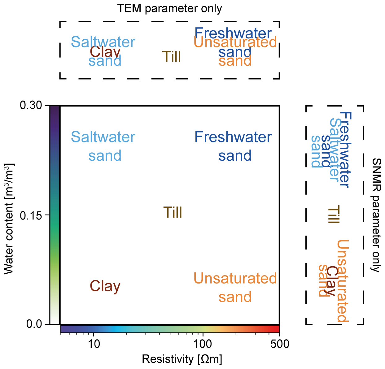
Figure 1 Different hydrogeological units resolved with TEM and SNMR. In dashed boxes, only one method is used, and the overlapping units show the ambiguities found. $T_{\mathrm{2}}^{\ast }$ can be implemented to further separate units. Colors in text are not related to color bars.

A multiple-data-type approach requires forming interpretations consistent with multiple geophysical model types simultaneously, which can be achieved through manual inspection of disparate data types. This enables one to distinguish hydrogeological layers through combined interpretation of all data types but requires subjective choices regarding boundary delineation. Others have used a joint inversion approach where layer boundaries are set using multiple geophysical methods (Günther and Müller-Petke, 2012; Behroozmand et al., 2012). The joint approaches have the ability to delineate layer boundaries not seen when inverted separately. An alternative approach employs statistical correlations across separate parameters to partition these into different clusters. One such approach is K-means clustering, which enables the subdivision of datasets based on multiple parameters (Kodinariya and Makwana, 2013). Different clustering approaches have also previously been applied to geophysical data and focus primarily on single source datasets, such as large EM datasets (Dumont et al., 2018) or large electrical resistivity datasets (Song et al., 2010). Some studies investigate clustering on derived parameters such as clay fraction and resistivity, both linked to EM surveys (Foged et al., 2014). Clustering across disparate data types, such as Bouguer anomaly data and magnetic data, has been shown to improve the resolution of mineral deposits (Sun and Li, 2016). A study focused on delineating structures in urban settings by clustering on multichannel analysis of surface waves (MASW) and electrical methods to evaluate soil foundation structure (Le et al., 2022) and found the K-means clustering to resolve important structures in the shallow subsurface.

In this study, we demonstrate the benefits of combined SNMR and TEM data collection, where K-means clustering based on coincident models in two survey areas is shown to enhance interpretations and address ambiguities that persist if only a single data type is considered. The first example includes mapping of the water table in an unconfined meltwater plain aquifer, where a combined approach is used to address ambiguity as to the upper aquifer being confined, unconfined, or semi-confined across the investigated region. A second example taken from a small island shows how the method can delineate saltwater intrusion from clay-rich regions through a combined interpretation. We demonstrate a workflow for handling interpretations of SNMR and TEM simultaneously, reducing possible interpretational bias.

2 Methods

2.1 Transient electromagnetic

In this study we use transient electromagnetics (TEM) to resolve subsurface resistivities. The tTEM instrument (Auken et al., 2019) was used in both field areas and can resolve the resistivity structure of the top 70 m; however, here only the top 25 m of the full model domain is used in the analyses. The induced voltages recorded by the tTEM are translated to 1D resistivity models by spatially constrained inversion (SCI) using Aarhusinv (Auken et al., 2015; Viezzoli et al., 2009). The model is discretized into 30 layers with thicknesses varying from 1 m shallowly to 10 m at depth following resolution limitations at depth. The resulting resistivity models will be used for subsequent clustering.

2.2 Surface nuclear magnetic resonance

In this survey we use a recently developed technique for SNMR called steady state. The steady state has an increased stacking rate, leading to a higher signal-to-noise ratio and a decrease in acquisition times (Grombacher et al., 2021). A set of transmit pulses, optimized to resolve the top 25 m, was employed in both studies with the Apsu instrument with an acquisition time of 25 min per site (Larsen et al., 2020). The resolved water content and the relaxation parameter, $T_{\mathrm{2}}^{\ast }$, are used in the subsequent clustering. The data are also inverted for T₂, more directly linked to pore geometry, but are not used in the subsequent clustering. The SNMR models are discretized into 31 layers down to 50 m, increasing in thickness at depth from 0.5 to 4 m. The resistivity structure from the nearest TEM sounding is used for the inversion. Resistivity is needed to obtain the excitation fields used for kernel calculations (Braun and Yaramanci, 2008).

One limitation in SNMR is to detect water residing in very small pores. Because of instrument dead times associated with transmitting the excitation pulse (on the order of 8 ms), receiving data immediately after pulse termination is not possible. $T_{\mathrm{2}}^{\ast }$ relaxation time is linked to pore sizes with low values occurring in small pores, while large pores have large values. Signals from very small pores can therefore partially or fully decay, i.e., lose their amplitude and coherency, before the instrument has begun recording data. As such, the magnetization from water residing in very small pores decays prior to data recording, which prevents observation of small pore water in SNMR. As such, SNMR water contents can be interpreted as a measure of “free” water or an effective porosity.

2.3 Inversion considerations

Traditionally, 1D SNMR inversions are most commonly treated separately as limited measurements are carried out. However, recent acquisition speed-ups enabled by steady-state approaches have significantly enhanced spatial data density, which enables the use of horizontal constraints linking inversions of nearby measurement sites (Grombacher et al., 2021). One such example is the use of laterally constrained inversion (LCI) for SNMR as proposed by Behroozmand et al. (2012) where neighboring sites in a transect can be connected. Here, we add a dimension to the constraints using a spatially constrained inversion (SCI) framework, to bind not only models in line, but all neighboring models. Delauney triangulation is used to find the relevant neighbors as in Viezzoli et al. (2009). The strength of lateral bounds is scaled by the distance between models, with a maximum strength defined when models are closer than a threshold distance. This threshold distance is typically set to the nominal or average distance between neighboring soundings (Vang et al., 2025).

The computational load increases immensely when implementing SCI with many layers and parameters. To reduce the number of iterations, the SCI starting models are defined by single-site inversion results. This allows the SCI to converge within a few iterations. The TEM data are inverted separately with an SCI for the entire survey.

2.4 Clustering

Large datasets enable statistical approaches to provide information on significant hydrogeological units. In the following examples, datasets are composed of 50 and 51 coincident SNMR/TEM soundings where a K-means clustering is employed (Kanungo et al., 2002) on their model parameters. The first step in this type of clustering is to select the number of clusters, K, into which the datasets will be clustered (Kodinariya and Makwana, 2013). After selecting the number of clusters, the algorithm makes an initial guess for the position of each cluster center in the parameter domain. The Euclidean distance from each data point to the cluster center is calculated, and each data point is assigned to the nearest cluster. The total distance from all data to their assigned clusters is then iteratively minimized through updating cluster center locations until either the centroid difference between iterations varies below a set tolerance or a maximum number of iterations is reached.

To improve clustering of datasets for parameters exhibiting different sensitivities and spanning different ranges, normalization was used to ensure that each parameter has the same weight in the clustering algorithm. Here, we use a Z score for normalization, where x is either resistivity (ρ), water content (WC), or relaxation parameter ($T_{\mathrm{2}}^{\ast }$):

$$\begin{array}{}\text{(1)}& x_{i,\mathrm{norm}}={\displaystyle \frac{x_i-\frac{\mathrm{1}}{n}\sum _{i=\mathrm{1}}^n{x}_i}{\mathit{\sigma }}},\end{array}$$

where σ is the standard deviation of the cloud of parameters from the inversion, x_i is the parameter value for the ith data point, and n is the number of data points. Following the normalization, we use the Scikit learn package in Python for the clustering and silhouette analysis (Pedregosa et al., 2011).

In this study, the number of clusters is chosen based on the silhouette index, which calculates the membership S_i of each data point, i:

$$\begin{array}{}\text{(2)}& S_i={\displaystyle \frac{b_i-a_i}{max(a_i,b_i)}},S_i\in [-\mathrm{1},\mathrm{1}],\end{array}$$

where a_i is average distance from data point i to other data points in the same assigned cluster, and b_i is the minimum average distance of the ith data point to all other data points in other clusters. The resulting index, or membership score, is a measure of how well a data point is associated with the assigned cluster. If the score of a given data point is 1 it indicates that the data point is correctly assigned, while a score of −1 indicates that the data are wrongly assigned (Kodinariya and Makwana, 2013; Shutaywi and Kachouie, 2021). By evaluating these results, we can qualify the preferred number of clusters. The preferred number of clusters is chosen based on two criteria. Firstly, the highest average silhouette index indicates that data points in general have the highest membership score with the given number of clusters. Secondly, we look at each cluster and their silhouette index. If more than 50 % of the cluster is above the average silhouette index, the cluster is well-defined, between 30 %–50 % the cluster is moderately defined, and below 30 % it is poorly defined. In some cases, prior information can be used to fix the number of clusters, such as prior geological knowledge of the area (Dumont et al., 2018).

In this study we clustered on three parameters: WC, $T_{\mathrm{2}}^{\ast }$, and ρ. The two geophysical methods used in this study have different sensitive volumes. SNMR inversion is discretized finely with 30 layers down to 50 m and the TEM has 30 layers in 120 m. To cluster on coincident values, a projection and averaging of the TEM ρ models onto the SNMR discretization is used. All TEM soundings within 60 m of an SNMR sounding are included. If there is no ρ model (TEM sounding) within 60 m, the nearest is used and mapped onto the SNMR discretization. This allows all SNMR points to be matched and prevents a reduction in data points.

2.5 Field site description

Two field surveys were conducted in different geologies to evaluate the use of clustering as a tool for alleviating interpretational ambiguity. Both sites were examined thoroughly with SNMR and TEM to provide the basis for the subsequent clustering analysis.

2.5.1 Kompedal

The first field site is Kompedal, a national forest in the Central Region, Denmark. The local geology consists of meltwater sand and glacial tills with varying clay contents. The sparse borehole coverage finds sand shallowly, and the water table varies from 5 to 12 m in depth. Two geophysical surveys have been conducted here using TEM and SNMR, respectively. The scope of the surveys was to delineate the water table on a regional scale and assess whether the shallow aquifer can be considered unconfined or semi-confined across the region. The TEM data were collected with the tTEM instrument (Auken et al., 2019) while driving along the gravel roads within the forest, as seen in Fig. 2a in blue. ρ values in the area are generally high, above 200 Ωm, with some layers of lower ρ found at depth. There is little to no contrast between the unsaturated and saturated part of the meltwater sand in ρ. The SNMR survey consists of 50 soundings acquired over 5 d in June 2021, spread across the forest as seen in Fig. 2a (Vang et al., 2023). The SNMR survey found low WC (∼5 %) and low $T_{\mathrm{2}}^{\ast }$ values (∼0.1 s) shallowly, with a sharp increase to higher WC (∼25 %) at 6 to 10 m depth. Layers with low WC and $T_{\mathrm{2}}^{\ast }$ can be associated with both unsaturated sands and clay-rich material. The section indicated in Fig. 2a will be used to show the results of the combined cluster analysis.

2.5.2 Endelave

The second location is a small 13 km² island, Endelave, in Kattegat, Denmark, with a maximum elevation of 8 m. The island's geology consists of glacial till, meltwater sands, and post-glacial sands, while boreholes intercept Paleogene clay at depth throughout the island. Generally, the glacial tills are found in the west part of the island, while the post-glacial sands are found to the north. TEM and SNMR surveys shown in Fig. 2b were conducted at this more geologically heterogeneous location to resolve possible saltwater intrusion and delineate the shallow aquifer found in the meltwater sands and tills. The TEM data were acquired in April 2022, cover the majority of the island, and show ρ below 150 Ωm for the entire area (McLachlan et al., 2025). The ρ values resolve buried valley structures and a very conductive basement. With TEM alone it is not possible to distinguish Paleogene clay from the saltwater-saturated sand. The SNMR survey consists of 51 soundings over 8 d in July and October 2023 and finds high WC shallowly in the east and north part of the island, while the west part shows low WC and $T_{\mathrm{2}}^{\ast }$.

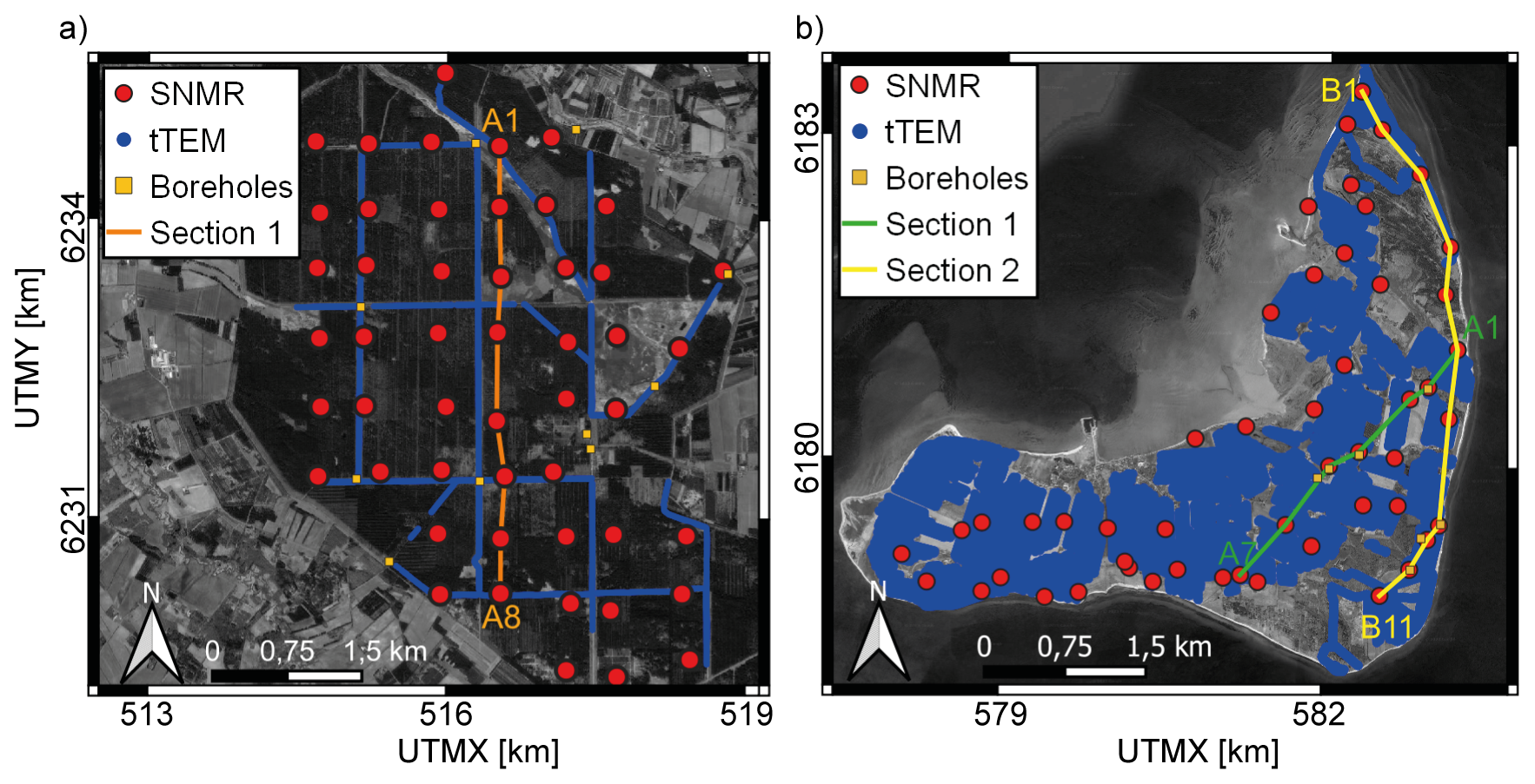
Figure 2 (a) The Kompedal survey area. SNMR (red) together with TEM (blue) was collected in the area. (b) Map of Endelave survey with SNMR (red) and TEM (blue). Map data: © Google Maps 2024, UTM zone: 32° N.

3 Results

3.1 Kompedal case study

3.1.1 Clustering analysis

For our combined analysis, we begin by selecting the number of clusters, K, using the silhouette index. Figure 3 shows results from four different clustering analyses with two to five clusters for the Kompedal dataset. Each cluster is labeled with its index and the number of data points within each cluster. In each cluster, the silhouette indices are sorted to give a higher index when moving up the y axis. We use the distinction of well-defined, moderately defined, and poorly defined, subdivided as mentioned in the Methods section. In the two-cluster analysis in Fig. 3a, we see that both clusters are well-defined with more than 300 members in each and could be a well-suited number of clusters. With three clusters (Fig. 3b), cluster 1 is moderately defined, while cluster 2 is poorly defined with many data points having a below-average silhouette index, and cluster 3 is well-defined. In the four-cluster analysis, two clusters, cluster 1 and cluster 4, become poorly defined, as seen in Fig. 3c. Lastly, five clusters yield three poorly defined clusters (2, 3 and 4) with only a few data points having a high membership score. The total average silhouette index indicated by the gray line highlights that either two or three clusters should be used. Prior hydrogeological information can be used to further qualify the choice between these (Dumont et al., 2018), and in Kompedal, we expect three distinct hydrogeological units: unsaturated sand, saturated sand, and underlying till. The low silhouette indices in cluster 2 in Fig. 3b are a product of large variation within the cluster, which can be expected in glacial environments as mixing occurred during deposition. Finally, three clusters were chosen to subdivide the data into meaningful and decently determined clusters.

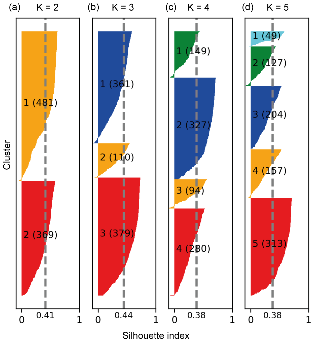
Figure 3 Silhouette index analysis for the Kompedal dataset. Four clustering routines were run with different numbers of clusters, K: (a) two, (b) three, (c) four, and (d) five. The sorted silhouette indices are shown for each cluster, with the average index indicated by the gray dashed line.

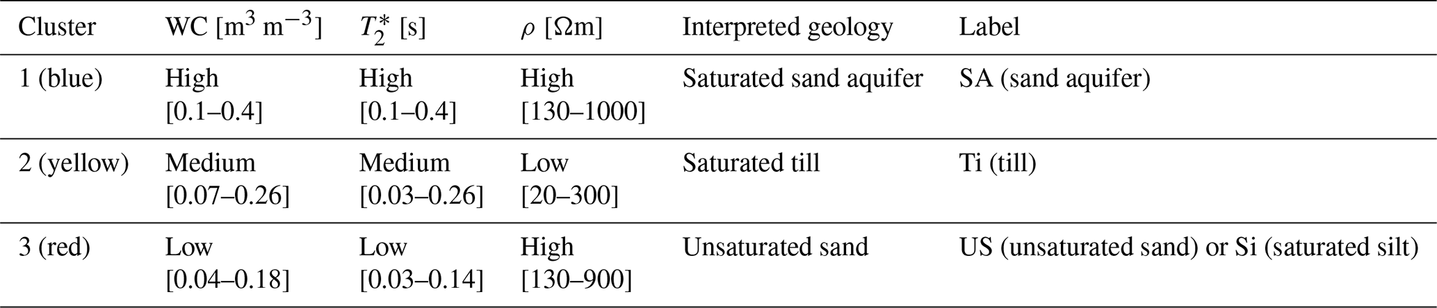
Given three clusters, K-means clustering is used to partition the model parameters, WC, $T_{\mathrm{2}}^{\ast }$, and ρ. In Fig. 4a, the three model parameters are shown in a scatter plot where the color of a point reflects the assigned cluster. The other three 2D scatter plots in Fig. 4b, c, and d show the clustering results projected onto a plane that reveals correlations between two of the three. Cluster 1 in blue is characterized by high WC, a high $T_{\mathrm{2}}^{\ast }$ value, and high ρ. Table 1 shows that large variation occurs within this unit in the SNMR parameters as seen in Fig. 4b. The unit is interpreted as a sandy aquifer given its high WC, high $T_{\mathrm{2}}^{\ast }$, and high ρ. The very high ρ (above 300 Ωm) is a product of very coarse material and the fact that the TEM method can have limited sensitivity to determine resistivity above 150 Ωm (Christiansen et al., 2006). The yellow cluster, cluster 2, has the largest variation in ρ (hence the low average silhouette index) but generally has lower ρ values than the other two clusters seen in Fig. 4c, with a large range in WC. A layer with these signatures is consistent with a saturated sandy till to a more clay-rich till, with low ρ. The overlap with cluster 1 in WC and $T_{\mathrm{2}}^{\ast }$ in Fig. 4b is interpreted as a gradual mixing of till and sands. Cluster 3 in red has low $T_{\mathrm{2}}^{\ast }$, low WC, and high ρ, which corresponds to unsaturated sand. However, low SNMR parameters and high ρ could indicate a silty deposit with smaller pore sizes, but with a similar conductivity. In places where the red cluster is found shallowly, it is interpreted as unsaturated sand, and at depth under the water table, it is interpreted as saturated silt.

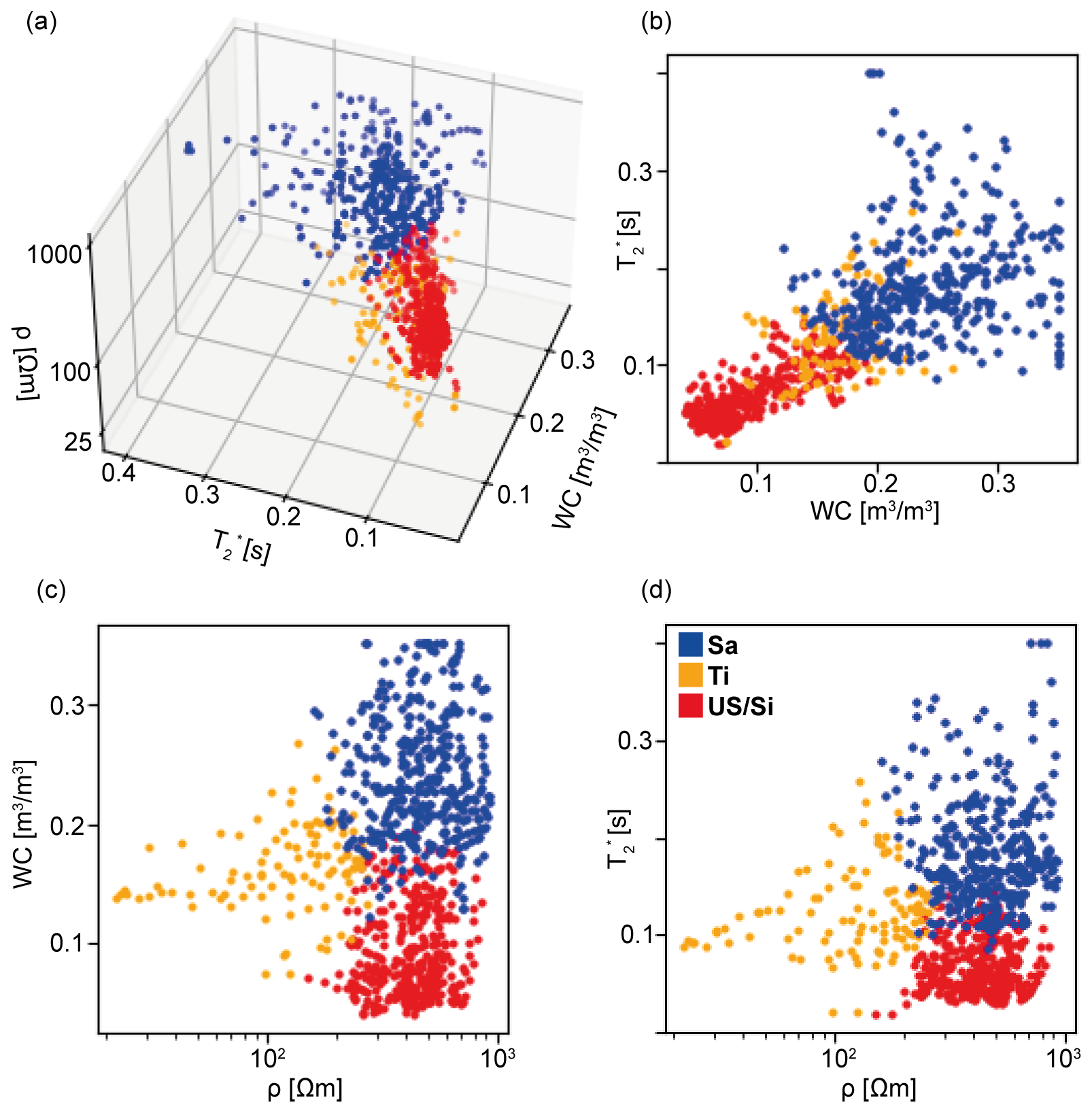
Figure 4 Clustering results from the Kompedal survey for three parameters: WC, $T_{\mathrm{2}}^{\ast }$, and ρ. (a) All three parameters in a scatter plot: (b) WC and $T_{\mathrm{2}}^{\ast }$, (c) ρ and WC, and (d) ρ and $T_{\mathrm{2}}^{\ast }$. The color of each data point defines the assigned cluster (1: blue, 2: yellow, 3: red) and their interpreted geology seen in Table 1.

Table 1 Cluster parameter bounds and interpreted geology for Kompedal.

3.1.2 Spatial interpretation

The three clusters are described in Table 1 and will be referred to by their labels, which are used in the figures to highlight their spatial extent. After assigning interpreted geologies to each cluster, we focus on their spatial position illustrated by a cross-section (location shown in Fig. 2a). Consider section 1 in Fig. 5, where the coincident data used in the clustering are shown as bars with colors associated with the assigned cluster. The US/Si cluster is situated mostly in the shallow subsurface extending from the surface down to depths of 5 to 10 m. The gray lines track selected cluster boundaries at the sounding locations. The upper gray line in Fig. 5 tracks the bottom of the US cluster and is interpreted to be a change from low to high saturation, since the US cluster is defined by low WC and the underlying clusters have a higher WC. The SA cluster is found in most soundings and has a variable thickness from 2 to 17 m. The transition at sounding location 8 is from the US to Ti cluster, likely due to lower ρ in this area. A second deeper gray line tracks the transition below the SA cluster to the underlying Ti cluster.

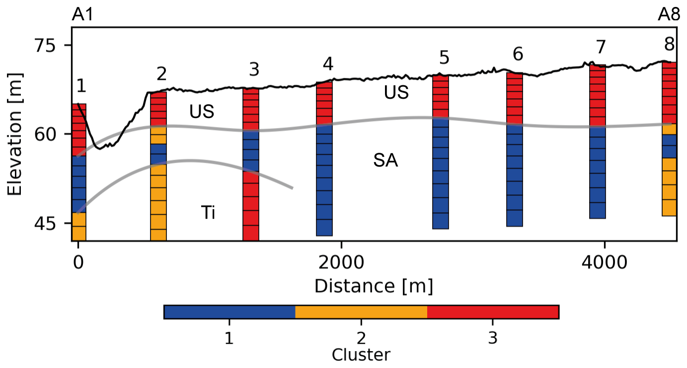
Figure 5 Clustering section from Kompedal where the partitioning of data is shown at every sounding. The gray lines track selected cluster boundaries. See Table 1 for cluster descriptions. A increases in the south direction.

To evaluate possible variations within the boundaries estimated from the clustering, the profile shown in Fig. 5 is reproduced in Fig. 6 with ρ values and WC and $T_{\mathrm{2}}^{\ast }$. Since clustering is a discrete and often brutal partitioning of smoothly varying parameters, it is important to return to the original parameters for evaluation. The SNMR WC values are shown as bars in Fig. 6a, and both $T_{\mathrm{2}}^{\ast }$ (left part of the bar) and T₂ (right part of the bar) are shown side by side with the same color scale in Fig. 6b and will be referred to as $T_{\mathrm{2}}^{\ast }/T_{\mathrm{2}}$ profiles. The gray lines from the clustering are superimposed on this section to track variations within each cluster unit. Figure 6a displays the first section where shallow low WC and high ρ coincide with the US cluster where the $T_{\mathrm{2}}^{\ast }/T_{\mathrm{2}}$ profiles show low values. Boreholes identify this unit as sand near sounding locations 3 and 6, which match the interpreted geology as an unsaturated sand. The upper gray line tracks an increase in WC from ∼15 % to ∼30 % in Fig. 6a and from below 0.1 s to above 0.15 s in $T_{\mathrm{2}}^{\ast }$ in Fig. 6b, while there is no contrast in ρ. The lack of structure in the ρ indicates that the TEM is not sensitive enough to track this saturation change, whereas a lithological change would generally be expected to coincide with a larger ρ contrast, visible in the TEM data. The elevated $T_{\mathrm{2}}^{\ast }$ is caused by less interaction of excited hydrogen spins with the grain surfaces because of increased saturation in the sand (Falzone and Keating, 2016). Additionally, a borehole water table measurement coincides with this transition line at sounding location 6. The SA cluster unit contains a range in WC from 20 % to 30 % and in $T_{\mathrm{2}}^{\ast }$ from 0.15 to 0.3 s, indicating slight variations within the cluster. The SA–Ti transition coincides with a decrease in WC and ρ, interpreted as a similar reduction in pore size, a product of an increase in fine content. The $T_{\mathrm{2}}^{\ast }$ values found in the Ti cluster, while quite varying, are generally lower than in the SA cluster, consistent with the interpretation of increasing fine content at depth, as in a till.

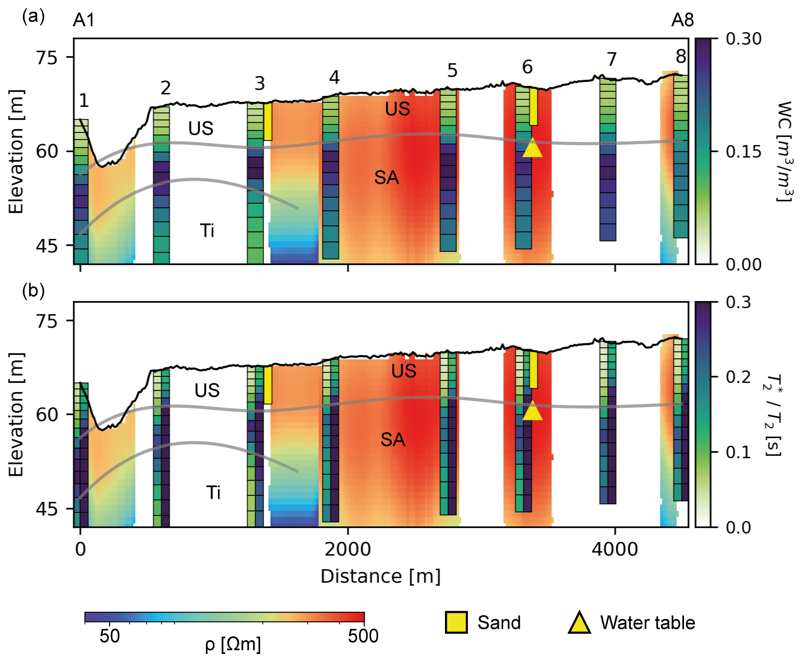
Figure 6 Profile of eight SNMR soundings (bars) and the TEM profile (background): section 1 in Fig. 2a. (a) SNMR WC and (b) a split bar with $T_{\mathrm{2}}^{\ast }$ (left) and T₂ (right). Boreholes at sounding locations 3 and 6 are shifted ∼40 m to avoid overlapping with the bars. Gray lines track transitions between clusters in Fig. 5. A increases in the south direction.

To further evaluate the accuracy of the ability to track water tables by the upper cluster transition, consider Fig. 7, where water tables from clustering are compared to available borehole-measured water tables within 500 m of SNMR sites. The clustering water tables are picked as the transition from the low-WC US cluster to any underlying cluster, SA or Ti, as both have a high WC compared to the US cluster. The red line has a slope of 1 and the uncertainty bars are equal to the inversion layer thickness at the transition depth, as the clustering method is ternary (i.e., it has three options), and consequently, some layers found at cluster transitions could be assigned to either cluster. We see that clustering tends to overestimate the water table elevation in many cases. This is a product of clustering being a brute thresholding in the parameter space. In this geology, the threshold from the clustering occurs at slightly lower WC than those coinciding with the water table and produces estimates that are too shallow. The trend, however, is similar to a slope of 1, indicating that a higher threshold could provide a better resolution of the regional water table. Additionally, the distance between the borehole and coincident SNMR and TEM models could add uncertainty for the comparison, but this uncertainty is expected to follow the slope of 1. Overall, the clustering captures the water table trend within an unconfined aquifer at a regional scale in an automated manner.

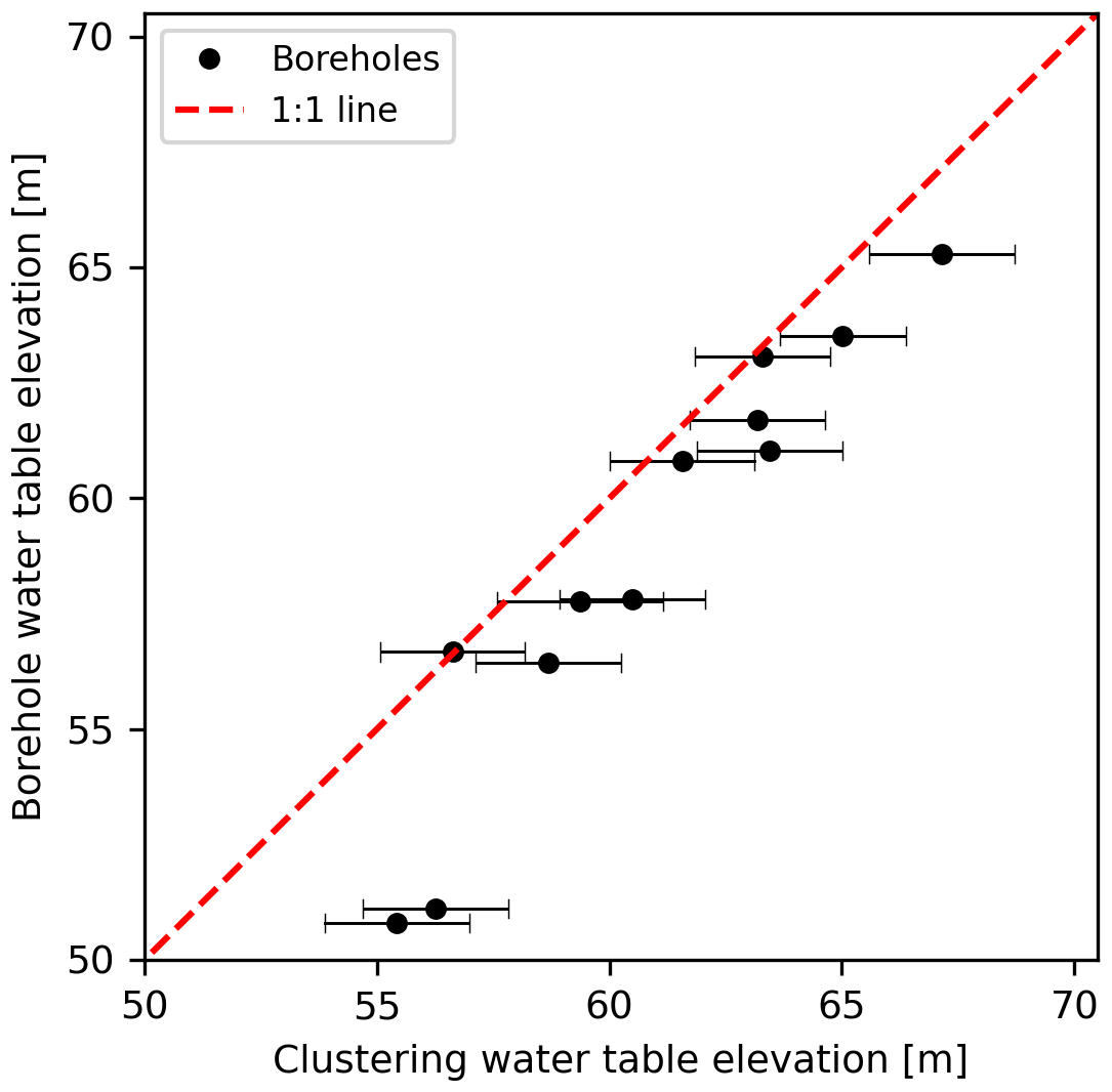
Figure 7 Borehole water table compared to the clustering water table at 12 SNMR locations with boreholes within 500 m. The red line has a slope of 1 and the error bars of the clustering estimates represent the inversion layer thickness just below the water table estimate to demonstrate the uncertainty related to the discretization of the resulting model.

3.2 Endelave case study

3.2.1 Clustering analysis

As before, we start by selecting the appropriate number of clusters through silhouette index analyses, shown in Fig. 8. Considering we expect a more heterogeneous geology, three to six clusters are used in the analysis. In Fig. 8, three clusters are used to partition the data and result in one well-defined, one moderately defined, and one poorly defined cluster, whereas the yellow has low and even negative silhouette indices, indicating wrongly assigned data points. The average silhouette index is the highest found with the assigned clusters. By using four clusters in Fig. 8, two are well-defined, one moderately, and one poorly clustered. We see less negative silhouette index data here, while still maintaining a high average silhouette index. Further increasing the number of clusters to five reveals similar silhouette indexes but has two moderately defined clusters; however, the average silhouette index drops (see Fig. 8c). Using six clusters is similar with a few well-defined and moderately defined and with a lower average silhouette index. The silhouette analyses show that the number of clusters should either be three or four as they have well-partitioned clusters, with the highest silhouette index. Prior information from the area indicates that we have four distinct geological units: tills, sand aquifers, Paleogene clay, and possible saline intrusion into sand. The blue cluster in Fig. 8b was found to have important hydrogeological information, regardless of its low silhouette index, and, as such, we used four clusters for further results.

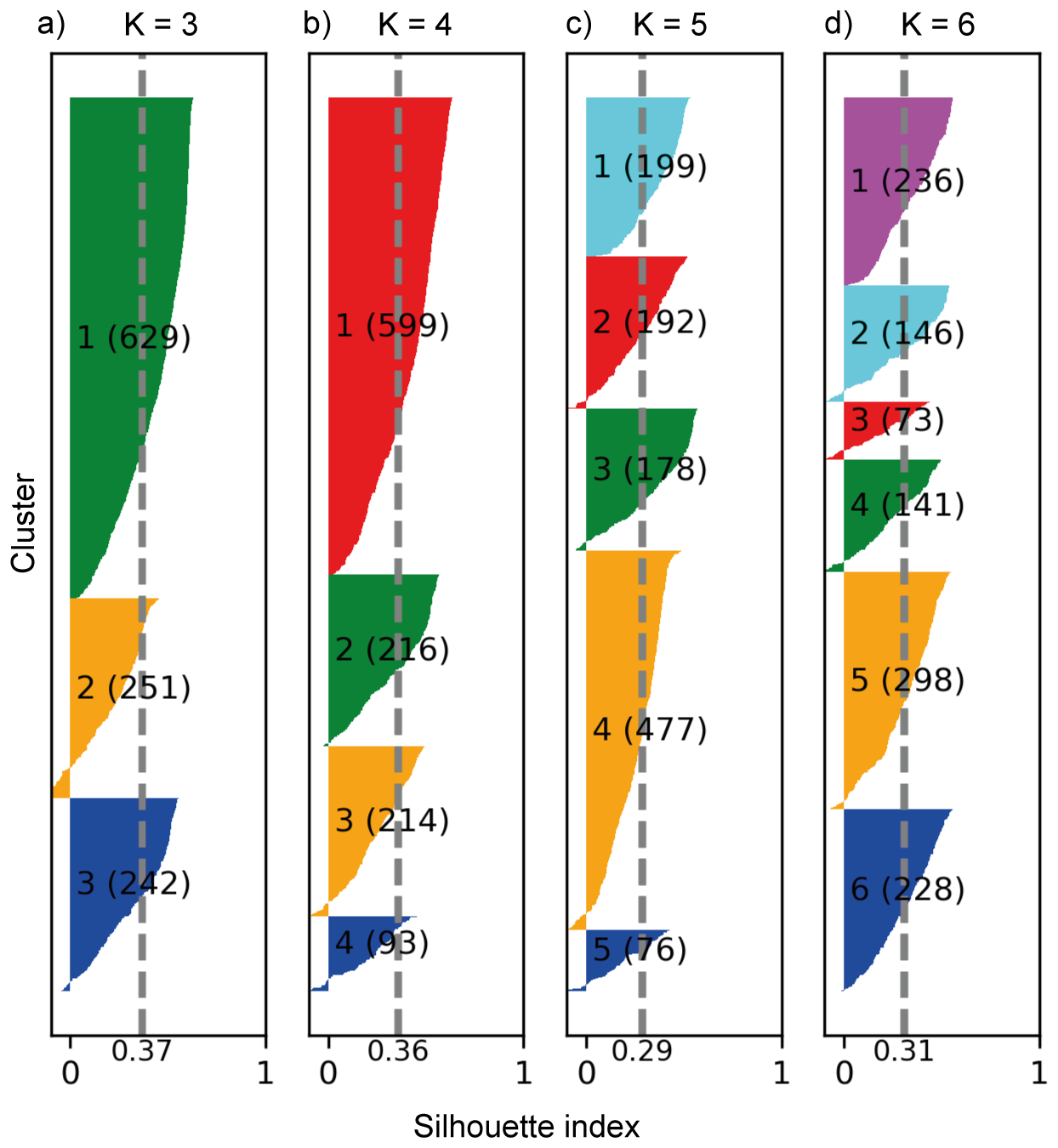
Figure 8 Silhouette index analysis for the Endelave dataset. Four clustering routines were run with different numbers of clusters, K: (a) three, (b) four, (c) five, and (d) six. The sorted silhouette indices are shown for each cluster, with the average index indicated by the gray dashed line.

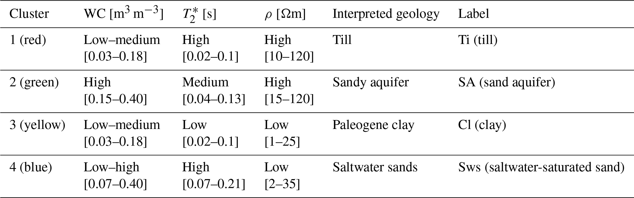
Next, the partitioning of WC, $T_{\mathrm{2}}^{\ast }$, and ρ is inspected in Fig. 9. First, the red cluster (1) is defined by quite low WC and $T_{\mathrm{2}}^{\ast }$ values (Fig. 9b), while the ρ varies from 10 to 120 Ωm. This cluster exhibits properties consistent with till containing varying sand content and affecting ρ (Fig. 9c). The green cluster (2) has mainly high ρ, high WC, and medium $T_{\mathrm{2}}^{\ast }$ values in Fig. 9a. The high WC and ρ are properties associated with saturated sand aquifers. The yellow cluster (3) has similar SNMR attributes to the red cluster, with low WC and $T_{\mathrm{2}}^{\ast }$, but has a lower ρ range illustrated in Fig. 9d. This unit is interpreted to be of Paleogene clay due to the very low ρ found in this cluster. The range of WC found within the yellow cluster indicates that layers with low to medium sand contents, but with low ρ, are grouped here. The last cluster, blue (4), has a distinct $T_{\mathrm{2}}^{\ast }$ range in Fig. 9b and a large range of WC with ρ situated around 10 Ωm. The WC and $T_{\mathrm{2}}^{\ast }$ values indicate that this layer has aquifer properties usually associated with sand, while the ρ indicates this as a conductive material. This is interpreted as saltwater-saturated sand. In general, the clusters are not as distinct within the Endelave dataset, as the glacial interaction with the deposited sediment has caused a mixing of lithologies. This is evident from the ρ values where none exceed 130 Ωm, whereas the Kompedal survey consisted of ρ from 50 to 1000 Ωm. All the descriptions and interpreted geologies are found in Table 2.

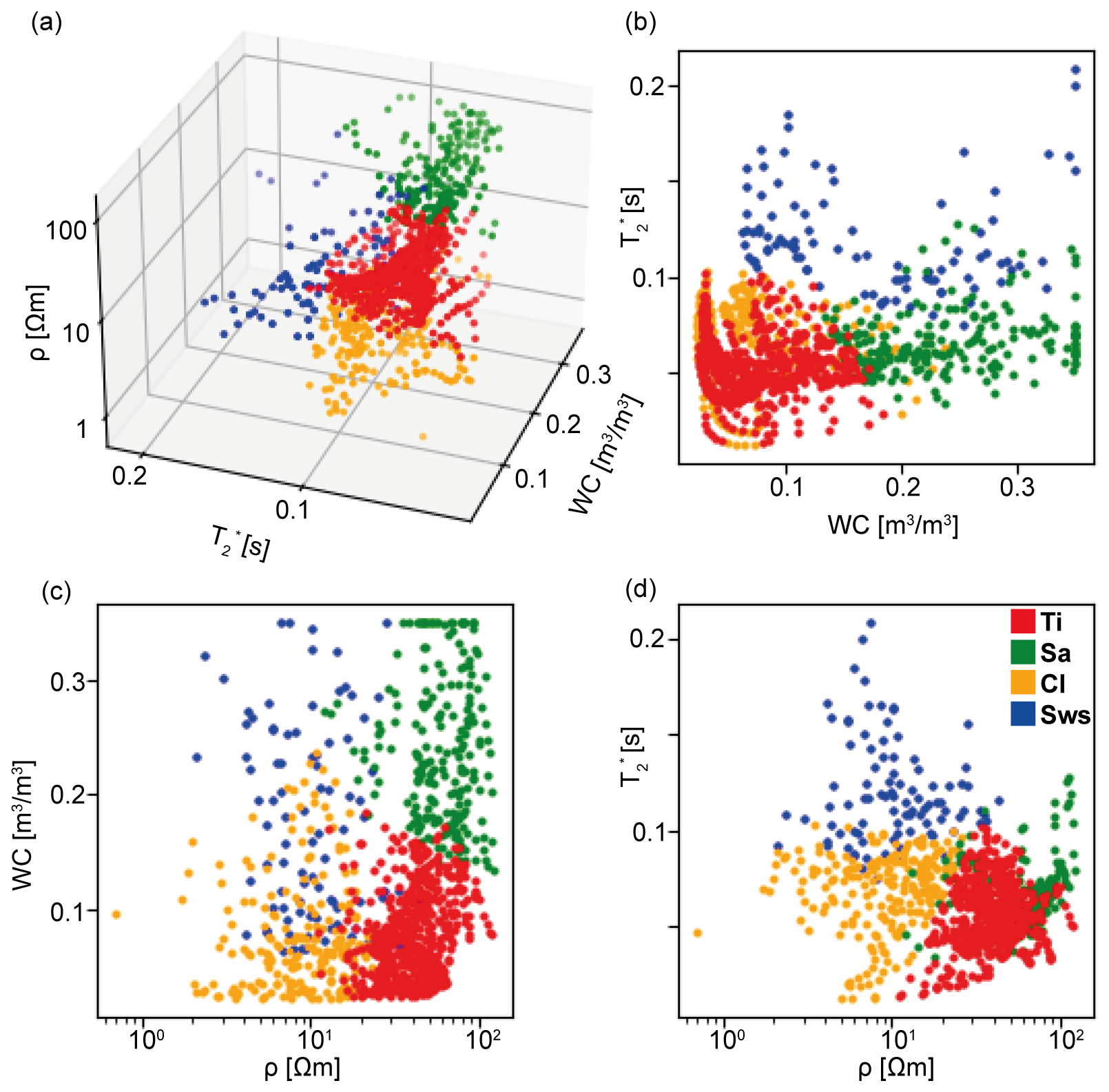
Figure 9 Clustering results from the Endelave survey for WC, $T_{\mathrm{2}}^{\ast }$, and ρ. (a) All three in a scatter plot: (b) WC and $T_{\mathrm{2}}^{\ast }$, (c) ρ and WC, and (d) ρ and $T_{\mathrm{2}}^{\ast }$. The color of each data point defines the assigned cluster and their interpreted geology; abbreviations can be seen in Table 2.

Table 2 Cluster parameter bounds and interpreted geology for Kompedal.

3.2.2 Spatial interpretation

Following the clustering we will examine their spatial extent on Endelave. We will show the results of two sections (Fig. 2b) to see how the clustering performs in a more heterogenous setting. Consider first the section across the main shallow aquifer in Fig. 10a, where we see a shallow Ti unit corresponding to either a till or unsaturated sand. The SA cluster unit has a thickness from 5 to 12 m and is found below the Ti cluster at sounding locations 3 to 6. Sounding location 1 is located 30 m from the coast, which aligns with the presence of the Sws cluster. The Ti cluster at depth is interpreted as a decrease in pore size from an increased clay or silt content. At sounding 7, all layers are grouped as the Ti cluster, a sign of low SNMR parameters throughout the entire sounding location. The deepest discretized layers at most sounding locations are grouped in the Cl cluster, tracked by a gray line, indicating a drop in ρ, as expected from the Paleogene clay.

To highlight possible saltwater intrusion, a section intersecting sounding locations at the coast is shown. The section in Fig. 10b is quite complicated as it transects different geological regions. We consider three main points in this section: the Sws cluster, the SA cluster, and the south end of the profile. In Fig. 10b we see the Sws cluster at sounding locations 1 to 3, defining a shallow and deep layer, while at sounding locations 6, 8, and 9 the cluster is seen shallowly at low elevations following the coast. The transition from the Sws cluster to the underlying clusters is tracked by a gray line at sounding locations 1 to 3. Below the gray line at sounding locations 1 and 2, the layers are grouped with the Cl cluster, representing low ρ and lower $T_{\mathrm{2}}^{\ast }$ and WCs. It is important to note that even with combined SNMR and TEM, it will be hard to distinguish between saltwater and freshwater clays as both will be conductive and have low free-water content and $T_{\mathrm{2}}^{\ast }$ signatures in SNMR.

From sounding locations 3 to 8, the SA cluster is found with a varying thickness from 2 to 10 m. This unit, interpreted as the aquifer, is outlined in gray to compare with original parameter values and borehole information later. At the south end of the profile, the clustering divides layers into Cl and Ti clusters, associated with clay and till by their low WC and $T_{\mathrm{2}}^{\ast }$.

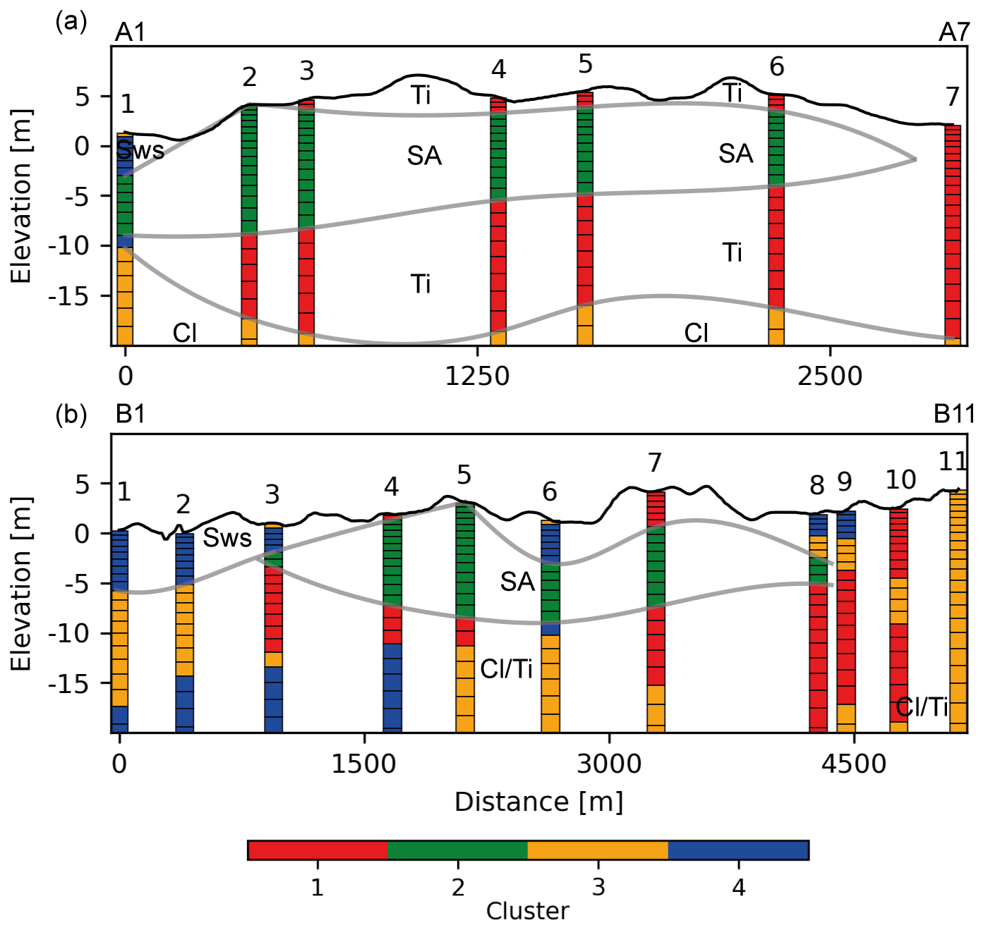
Figure 10 Clustering sections from Endelave where the partitioning of data is shown at every sounding location. (a) Section 1 and (b) section 2 in Fig. 2b. The gray lines track selected cluster boundaries. A increases in the southeast direction. B increases in the south direction.

The discrete boundaries from the clusters are now used in the original parameter space to evaluate possible variations within the clusters and the estimated boundaries. In Fig. 11, we consider the main shallow aquifer found on Endelave. The gray lines from Fig. 10a are used to delineate cluster extents and each unit is assigned a cluster label. Shallowly, the Ti unit coincides with low WC and a high ρ in Fig. 11a. $T_{\mathrm{2}}^{\ast }/T_{\mathrm{2}}$ values are low in this unit and boreholes reveal either till or unsaturated sand here, matching the clustering interpretation. The upper Ti–SA gray line tracks an increase in WC at four sounding locations, coincides with a lithological change from clay to sand in two boreholes, and coincides with a water table measurement in a separate borehole. This is interpreted as a semi-confined system with the water table coinciding with a lithological layer boundary. The SA unit here consists of high WC and low to medium $T_{\mathrm{2}}^{\ast }$ within a resistive unit. The boreholes identify this unit as sand or a mixture of sand and silt, which explains the range of WC grouped within this unit. The lower SA/TI transition tracks a decrease in WC, still with low to medium $T_{\mathrm{2}}^{\ast }$ as seen in Fig. 11b. The transition coincides with a decrease in ρ at sounding locations 1 and 2 and with a lithological boundary from sand to clay in a few boreholes. Furthermore, two boreholes terminate exactly at this interface, which could indicate that the drillers hit something harder or more clay-rich, prompting them to stop drilling. The Ti/Cl transition at depth tracks a decrease in ρ, which in the deep borehole is identified as a lithological boundary from clays and sand to Paleogene clay, agreeing with the clustering interpretations. This deep boundary is not seen in the SNMR parameters as the Ti and Cl clusters are only distinguishable by their ρ.

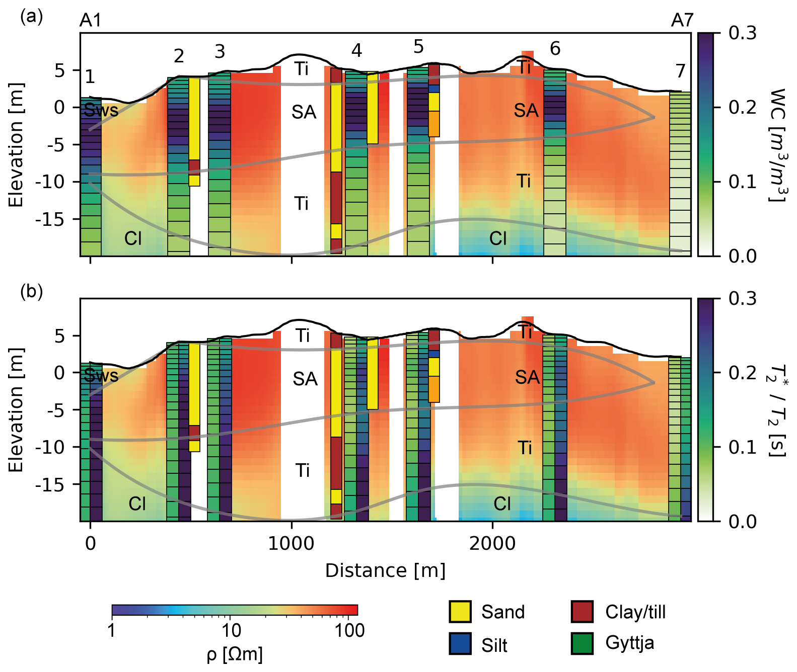
Figure 11 Profile of 7 SNMR soundings (bars) and TEM ρ (background): section 1 in Fig. 2b. (a) SNMR WC and (b) a split bar with $T_{\mathrm{2}}^{\ast }$ (left) and T₂ (right). Gray lines track transitions between clusters in Fig. 10. A increases in the southeast direction.

After reviewing the section through the main shallow aquifer in Fig. 11, we will assess a second, more complex section. The gray lines from Fig. 10b will be used to delineate the cluster units and illustrate differences within the units. Consider now Fig. 12, where the ρ and SNMR parameters are shown with lines following cluster transitions. The Sws unit is seen mainly at locations 1 to 3 and is defined by high WC, very high $T_{\mathrm{2}}^{\ast }$, and low ρ. At sounding location 8, a borehole finds sand coinciding with the Sws cluster, in agreement with the saltwater-saturated sand interpretation. The high $T_{\mathrm{2}}^{\ast }/T_{\mathrm{2}}$ associated with the Sws cluster in Fig. 12b is a product of limited compaction within the newly deposited sand in the coastal environments. Below the Sws unit, the gray line tracks a transition to lower WC and $T_{\mathrm{2}}^{\ast }$, but maintaining the low ρ, which is defined by the Cl cluster. At sounding location 6, this transition is different, with an increase in ρ tracking the border to the SA unit. Low WC at sounding locations 10 and 11 coincides with clay in a local borehole for the first 15 m where all layers are grouped within the Ti or Cl clusters. The low water content and $T_{\mathrm{2}}^{\ast }$ signature at these locations prevent them from being clustered with the saltwater-saturated sands in Sws, highlighting the value of SNMR to distinguish these conductive units. The gyttja layer found in the borehole coincides with a drop in the SNMR WC due to the increases in organic matter, decreasing the pore size, and it was grouped with the Cl cluster (Mashhadi et al., 2024).

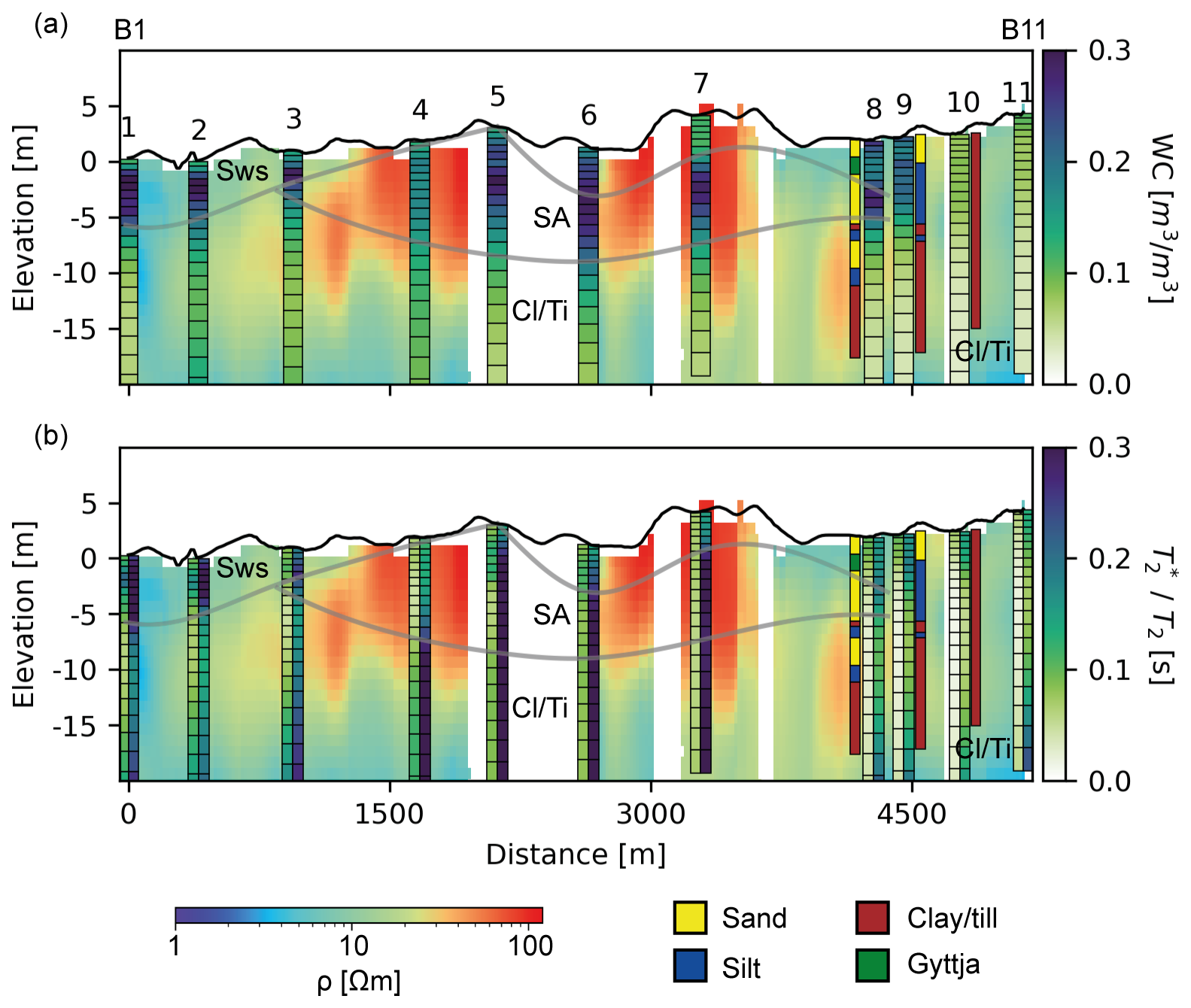
Figure 12 Profile of 11 SNMR soundings (bars) and TEM ρ (background): section 2 in Fig. 2b. (a) SNMR WC and (b) a split bar with $T_{\mathrm{2}}^{\ast }$ (left) and T₂ (right). Gray lines track transitions between clusters in Fig. 10. B increases in the south direction.

By clustering on this dataset, we have proven the ability to identify regions of possible saltwater intrusion. Figure 13 shows which sounding locations have layers that cluster within the saltwater aquifer, the freshwater aquifer, that have layers of both clusters, or only have the till and clay clusters. The saltwater cluster is observed mostly at the northern sounding locations where the post-glacial sands are located, but also along the east coast. The main aquifer unit, SA, is found in the east and north parts of the island, while the west part is dominated by the low-water-content clusters, shown in yellow and red. One sounding location with both saline and freshwater clusters far from the coast is observed in the north of the island. The closest TEM sounding was acquired in a lowland south of this sounding, with elevation almost at sea level, which might cause issues with saltwater intrusion. There is also a wetland close to this location, which might have a higher clay content with low ρ. If the TEM and SNMR are not exactly coincident, some differences and anomalies in the clustering might occur. But in general, the K-means clustering is able to map this possible saltwater intrusion, which is a valuable asset in aquifer management.

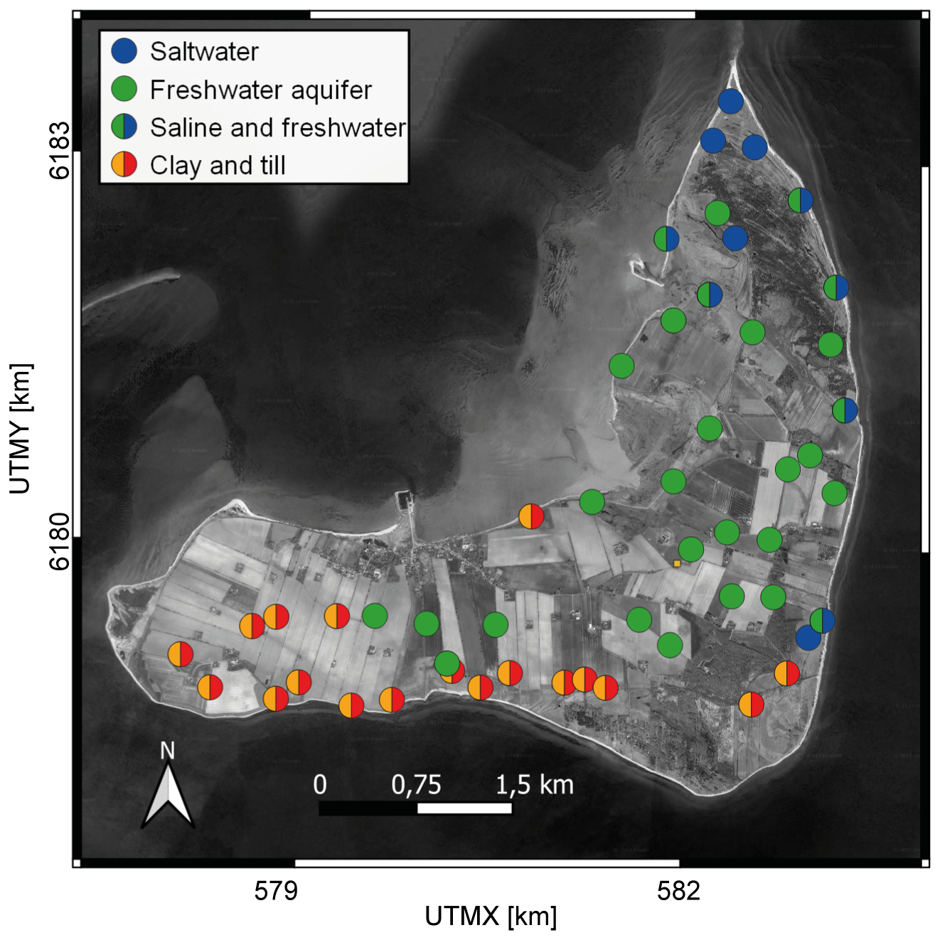
Figure 13 Sounding locations where saltwater or freshwater has been identified. Locations with only clay and till clusters are shown with red and yellow. Map data: © Google Maps 2024, UTM zone: 32° N.

4 Discussion

In this study we investigated the use of clustering to combine the analysis of two geophysical methods, SNMR and TEM. The K-means clustering was found to be able to differentiate units into interpretable hydrogeological layers and was consistent with manual interpretations. Combining the datasets helped alleviate some of the ambiguities found when interpreting one of the individual datasets alone, i.e., unsaturated/confined conditions in Kompedal and saltwater/freshwater in Endelave.

K-means clustering on geophysical models offers a simple, automated approach to identifying lithological transitions. It allows for reproducible boundary definitions without subjective interpretations of the geophysical models. Discretizing smoothly varying parameters into predefined clusters is, however, brutal and there will be variability within the unit definitions. The ability to return to the original parameter space with cluster boundaries is crucial in addressing subtle variations within units and can be used to evaluate cluster transitions.

K-means clustering applied to geophysical models is not limited to SNMR and TEM parameters; it can also be extended to other collocated datasets with distinct sensitivities. For example, in areas where a deep water table is expected within a sand layer, seismic methods may be appropriate. However, because the seismic velocity of saturated sands can be similar to that of clays or tills, incorporating collocated TEM models can help reduce interpretational bias. Similarly, relying solely on TEM data may make it difficult to detect the water table due to limited sensitivity to high-to-high resistivity contrasts.

In SNMR, correlations between WC and $T_{\mathrm{2}}^{\ast }$ may exist (Falzone and Keating, 2016). For example, in unsaturated sands, the low water content residing in the pores will be in close contact with the grain surfaces, resulting in a faster exchange of energy between excited hydrogen spins and pore walls, leading to low $T_{\mathrm{2}}^{\ast }/T_{\mathrm{2}}$. Since water content is proportional to signal amplitude, in low-WC environments, low signal amplitude results in reduced confidence in the $T_{\mathrm{2}}^{\ast }$ estimates. When such parameters are linked, it might be of interest to simplify the approach by clustering on the product of water content and $T_{\mathrm{2}}^{\ast }$. Thus, combining these two parameters may help reduce the influence of low-confidence $T_{\mathrm{2}}^{\ast }$ values in low-water-content environments. A similar option is to use a principal component analysis to reduce the basis to two parameters that describe most of the variance, which in the Kompedal case would be resistivity and the product of the SNMR parameters. However, in more complex geologies such as Endelave, a decrease in basis dimension may reduce the ability to distinguish layers of high WC and low $T_{\mathrm{2}}^{\ast }$ from layers with low WC and high $T_{\mathrm{2}}^{\ast }$. By examining the data's variation and correlation, we can make qualified decisions about whether to decrease the parameter space.

In this study, we focused on interpreting two survey areas using K-means clustering, which has proven to be sufficient in meaningfully partitioning data and identifying lithological boundaries. One feature of the employed K-means clustering approach is the need to specify clusters beforehand. In this study we based the choice of clusters on the silhouette index and prior geological information about the area. One alternative study uses agglomerative hierarchical clustering on SkyTEM data, which avoids selecting the number of clusters by starting with one cluster and subdividing until each data point has its own cluster (Dumont et al., 2018). This can alleviate some of the choices made for the silhouette index analyses and provides a better understanding of how clusters are further subdivided. A second challenge is to attribute uncertainties to the layer boundaries picked by the discrete K-means clustering. Here, others use fuzzy C-means where data points are assigned a membership score and can be partial members of more than one cluster (Paasche and Tronicke, 2007). Applying the fuzzy C-means can give an estimate of uncertainty for the picked cluster boundaries; i.e., if a data point could be a member of several clusters, it is less certain. This could apply to the Endelave data where the saline intrusion cluster in places could overlap with the freshwater cluster.

Another way of exploiting collocated datasets is the use of joint inversion for layer boundary picking. Studies identifying layers from SNMR and TEM implementing various regularization techniques have shown promise in reducing the ambiguity found when interpreting each separately (Behroozmand et al., 2012; Skibbe et al., 2018). These approaches focus mostly on the collocated datasets and invert these jointly. In our study, the tTEM data are inverted separately with the full survey of more than 23 000 datasets. As such, we have the ability to track the changes in resistivity in places where the SNMR is not present. Additionally, the framework for using joint inversion in steady-state SNMR is not established as kernels are calculated before the inversion, fixing the discretization. Further investigations could focus on implementing clustering in a joint inversion framework with a large spatial extent. This could alleviate some of the interpretational load when dealing with large datasets.

Since clustering is performed on coincident values, we are limited by the lowest-dimension dataset, which in this case is the SNMR; e.g., on Endelave the survey consists of 51 soundings, while there are over 23 000 TEM soundings in the same area. This reduction in data space disregards large amounts of TEM data, which of course have valuable regional information but lack coincident SNMR parameters. Additionally, lower data quantity can lead to clusters not representable for the area. If SNMR information could be extrapolated to the full TEM domain through appropriate spatially variable measures, it would allow for clustering on a much larger dataset. Future research will focus on extrapolating SNMR parameters across the full TEM domain. This would enable a subdivision of the full TEM domain based on the coincident data clusters, and it will be possible to better delineate areas of potential saline intrusion spatially.

As there is limited ground-truthing information, the clustering has been mostly compared to manual interpretations based on the data collected. This does not directly provide validation of the layers seen but indicates that the clustering is performing like expert interpreters would if given a similar dataset. As such this study shows the value in having clustering as the main subdivider of lithological units instead of having manual inspection of each collocated dataset. Given the recently enabled larger-scale mapping with SNMR, a less subjective and fast interpretation scheme is a step towards automation from data to lithology.

5 Conclusion

Through two field studies we demonstrated the automated spatial identification and separation of hydrogeological units in large-scale geophysical campaigns. Recent improvements in the data acquisition rates of SNMR now offer data volumes sufficient to exploit clustering approaches when combining these data with other geophysical data. K-means clustering of complementary SNMR and TEM models is shown to provide a less subjective approach, where enhanced hydrogeological interpretations can be formed by exploiting the complementary nature of two data types. To detect lithological boundaries, they must correspond to a contrast in geophysical properties. SNMR is shown to provide value when discriminating clay-rich sediments from saline-saturated sand conditions, a challenging task based on only TEM models. Similarly, TEM is able to separate low-water-content conditions from clay-rich conditions, which is impossible with SNMR alone. This is key to discriminating between unconfined and semi-confined conditions. A silhouette-index-based approach, combined with the a priori knowledge of the likely number of lithological units present, was used to select the number of clusters and found to be suitable for these datasets.

In the examples, clustering of NMR and TEM data provides a more complete characterization of local hydrogeological conditions than what can be achieved by each dataset separately.