Enhancing the performance of 1D–2D flood models using satellite laser altimetry and multi-mission surface water extent maps from Earth observation (EO) data

Digital elevation models (DEMs) are essential datasets, particularly for flood inundation mapping in one-dimensional (1D) to two-dimensional (2D) flood models. Given the significant uncertainties associated with DEMs that can affect flood modelling accuracy, minimizing these inaccuracies is essential. This study aims to improve the performance of 1D–2D flood models using satellite Earth observation (EO) data, focusing on the lower Chao Phraya (CPY) basin.

Two workflows are proposed: DEM analysis and flood map analysis. The DEM analysis evaluates 10 DEM products, including three local DEMs provided by Thai agencies (LDD, JICA, and a merged LDD-JICA DEM) and seven global DEMs derived from EO data (ASTER GDEM V3, SRTM V3, MERIT, GLO30, FABDEM V1–2, TanDEM-X, and TanDEM-EDEM). The evaluation process uses ICESat-2 ATL08 data processing, vertical datum reference processing, and evaluation of DEMs using ICESat-2 ATL08 benchmark processing. The DEMs are assessed using satellite laser altimetry data from the Ice, Cloud, and Land Elevation Satellite-2 (ICESat-2) as the benchmark. The evaluation employs standardized metrics, including point-wise, grid-wise, and track-wise comparisons, to identify the most suitable DEM for integration in the flood model. Results indicate that the merged LDD-JICA DEM and FABDEM V1–2 DEM exhibit the highest accuracy among local and global products, respectively, with root mean square errors (RMSEs) of 1.93 and 1.95 m, and percentage biases (PBIASs) of −15.38 % and 4.59 %.

The flood map analysis workflow involves comparing flood extent maps derived from multi-mission satellite datasets and simulated flood maps generated from 1D–2D flood models using the best available DEMs. This workflow utilizes surface water extent (SWE) maps from the WorldWater project, obtained from the Sentinel-1 and Sentinel-2 imaging satellites, and flood maps from the Geo-Informatics and Space Technology Development Agency (GISTDA) in Thailand to validate flood maps produced by the 1D–2D flood model based on the merged LDD-JICA DEM and FABDEM V1–2 DEM. The results reveal that flood maps based on the FABDEM V1-2 DEM slightly outperform those based on the merged LDD-JICA DEM, with an improvement of approximately 13.55 %–25.56 % in the critical success index (CSI). This study highlights the potential of leveraging satellite EO data to enhance the accuracy and reliability of 1D–2D flood models, thereby improving flood inundation predictions for effective flood management.

1 Introduction

Nowadays, flooding is one of the most common hazards globally, impacting health, economies, and livelihoods worldwide. Flood models play a crucial role in forecasting floods and assessing flood risks, thereby assisting decision-makers in effective water management, particularly through one-dimensional (1D) to two-dimensional (2D) flood models. These models simulate various aspects of flooding, including flow, water levels, flood inundation extents, flood depths, flood maps, and flood duration (DHI Water and Environment, 2019). The digital elevation model (DEM) serves as a primary input parameter for 1D–2D flood models, enabling accurate simulation of flood overflow from rivers, floodplains, and inundated areas, particularly in flat and low-lying regions. The DEM significantly influences the simulation of flood inundation in both 1D–2D and 2D flood models (Saksena and Merwade, 2015; Shen and Tan, 2020; Wu et al., 2007; Morrison et al., 2022) for urban areas (McClean et al., 2020), coastal areas (Darnell et al., 2008), and flood warning systems (Lamichhane and Sharma, 2018). Ultimately, the reliability of flood inundation predictions relies on the accuracy and resolution provided by the DEM, directly impacting the representation of flow geometry characteristics within flood models.

Currently, the advancements in survey technologies, such as unoccupied aerial vehicles (UAVs) (Perera and Nalani, 2022), light detection and ranging (lidar) (Raj et al., 2020), and mobile mapping systems (MMSs) (Schwarz and El-Sheimy, 2007), have significantly enhanced the accuracy, quality, and resolution of DEMs. These technologies enable the production of high-resolution terrain data; however, they remain costly, time-consuming, and less feasible for monitoring dynamic land-use changes or covering large river basins. For example, following the severe flooding in 2011, Thailand's Royal Irrigation Department collaborated with the Japan International Cooperation Agency (JICA) to survey a 27 000 km² area. This effort produced a high-resolution 2×2 m DEM and required approximately 7 months to complete (JICA, 2012), underscoring the significant resources needed for such large-scale surveys.

Earth observation (EO) technologies offer a promising alternative by providing global DEMs with comparable resolution and quality. EO-based DEMs, such as ASTER GDEM3 (Abrams et al., 2020), SRTMv3 (Farr et al., 2007), MERIT (Yamazaki et al., 2017), GLO30 (CDSE, 2022), FABDEMv1–2 (Neal and Hawker, 2023), TanDEM-X (Krieger et al., 2007), and TanDEM-EDEM, are freely available for download and utilize advanced techniques of EO and machine learning to generate elevation estimates. These satellite-derived DEMs cover remote or inaccessible areas, offering a cost-effective and efficient solution for generating high-resolution terrain data. Moreover, global DEMs derived from EO are increasingly being utilized as inputs for 1D–2D flood models, providing a practical and scalable option for flood risk assessment and forecasting in regions with limited resources.

However, validating the DEM before integrating it in the 1D–2D flood model is essential. The Ice, Cloud, and Land Elevation Satellite-2 (ICESat-2) is a satellite equipped with a laser altimeter, capable of measuring ice sheet and glacier elevation change, sea ice freeboard, land elevation, and water elevation (Neumann et al., 2019), providing opportunities for validating DEMs, even in remote and hard-to-reach areas worldwide, such as Finland (Wang and Liang, 2023), Spain (Zhu et al., 2022), east Antarctica (Hao et al., 2022), Alaska in the USA (Wang et al., 2019), and the Qinghai–Tibet Plateau in China (Weifeng et al., 2024). Additionally, ICESat-2 has been used to assess the suitability of global DEMs for hydrodynamic modelling in data-scarce regions (Nandam and Patel, 2024) and to enhance the accuracy of 2D hydraulic models in the upstream Yellow River (Coppo Frias et al., 2024). Moreover, while an efficient DEM enhances the efficiency of 1D–2D flood simulation, it is important to systematically validate flood maps. Currently, satellite earth observation (EO) data can be utilized for monitoring and providing surface water extent (SWE) with synthetic-aperture radar (SAR) sensors, such as RADARSAT (Raney et al., 1991), ENVISAT ASAR (Lv et al., 2005), COSMO-SkyMed (Pulvirenti et al., 2014), and TerraSAR-X (Martinis et al., 2013); this is the only way to validate flood inundation maps from flood models over regional scales. The WorldWater project developed a robust and scalable EO solution for inland SWE monitoring, which can be utilized by a large community of stakeholders involved in local water management (Tottrup et al., 2022). The project used free and open optical and SAR satellite imagery from the Sentinel-1 and Sentinel-2 missions to generate monthly SWE maps over 4 years, which are accessible from https://worldwater.earth/ (last access: 10 November 2023). The product offers new opportunities for validating modelled flood maps with higher SWE resolution.

While satellite EO provides SWE maps that delineate water bodies and inundated areas, they cannot be directly compared with flood maps from 1D–2D flood models. The outputs of 1D–2D flood models are riverine flood maps. Additional flood classification processing is necessary to ensure comparability between SWE maps and the output of a flood model. However, flood type classification using SWE maps poses challenges and difficulties. Many studies focus on classifying flood types based on meteorological condition rather than using SWE maps, for example, Nied et al. (2014) and Turkington et al. (2016), while others construct decision trees using meteorological data (Stein et al., 2019; Yan et al., 2023). Riverine flood classification specifically involves identifying floods caused by river overflow from SWE maps. Here, we used expanding segmentation labels (ESLs) (van der Walt et al., 2014), connected component labelling (CCL) (Rosenfeld and Pfaltz, 1966; AbuBaker et al., 2007), the masking of riverine and permanent water, and morphological image processing (MIP) techniques (Soille, 2003) applied to SWE maps to separate riverine flood areas from other inundated areas.

This study presents two new workflows supporting flood modelling and forecasting in the lower Chao Phraya (CPY) River basin in Thailand and elsewhere.

1. Comprehensive DEM evaluation. A detailed assessment of 10 DEM products, including 3 local and 7 global DEMs, was conducted using ICESat-2 as a benchmark for the Thailand domain. DEM performance in the lower CPY basin was evaluated using statistical methods, including bias (mean error, ME), mean absolute error (MAE), mean square error (MSE), and root mean square error (RMSE), with comparisons made at point and grid level, as well as track-wise comparisons. The highest-performing DEM from this evaluation was subsequently integrated in a 1D–2D flood model to simulate flood inundation.

2. Systematic comparison of flood maps. Simulated 2D inundation patterns were compared with flood maps derived from satellite EO-based surface water extent (SWE) using a riverine flood classification process.

The model's performance was assessed using three statistical metrics: probability of detection (POD), false alarm ratio (FAR), and critical success index (CSI). These methods will improve the performance of the operational hydrologic-hydraulic forecasting system for the Chao Phraya River, managed by the Hydro-Informatics Institute (HII) in Thailand.

2 Study area

The study area is located in the central part of Thailand, as shown in Fig. 1a. The delta area of the lower CPY River basin in Thailand forms the study area, depicted in Fig. 1c. The size of the study area is approximately 16 643 km², including about 70 % irrigation area and 20 % urban area. The topography of the study area is characterized by a flat terrain, predominantly consisting of a low-lying alluvial floodplain. To the north of the study area is a mountainous region with four main rivers: the Ping, Wang, Yom, and Nan rivers. These rivers converge to form the CPY River, which then flows into the study area. The eastern and western parts of the study area are connected to the Bang Pakong River and the Mae Klong basin, respectively. The southern part of the study area borders the Gulf of Thailand.

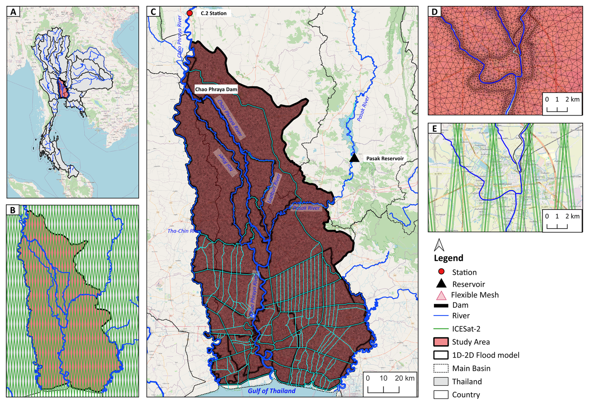
Figure 1 (a) The location of the study area, (b) the ICESat-2 orbit, (c) the study area/1D–2D flood model, (d) the flexible mesh in the flood model, and (e) ICESat-2 beam pairs. © OpenStreetMap contributors 2015. Distributed under the Open Data Commons Open Database License (ODbL) v1.0.

The study area is located in a tropical climate and is influenced by northeast and southwest monsoons. The northeast monsoon brings cool and dry air from November to February, while the southwest monsoon brings humid air from May to October. The precipitation is approximately 1100 mm during the rainy season and 170 mm during the dry season. The flooding in the study area is caused by the main rivers and their tributaries. The tributaries of the CPY River include the Tha-Chin, Noi, and Lopburi. Flooding problems are more severe along the main course of the CPY River compared with others. Nevertheless, flooding mechanisms are complicated, arising from the combined effects of extreme precipitation, river overflows, insufficient river conveyance, land-use change, and sea-level rise. This results in frequent flooding, as shown in Fig. 3c.

3 Materials

3.1 1D–2D flood modelling

In this study, we used the flood model from the decision support system for flood forecasting and water management in the CPY River basin, developed in collaboration with HII and DHI A/S since 2012 (Sisomphon et al., 2013) and updated with new information in 2016 (Charoensuk et al., 2018). The decision support system for flood forecasting and water management in the CPY basin continues to operate, supporting the Thai Government in managing flood risk and providing real-time flood forecasts.

The flood model uses MIKE FLOOD software, developed by DHI A/S. A MIKE FLOOD model (DHI Water and Environment, 2019) consists of coupled one-dimensional (1D) and two-dimensional (2D) models, namely MIKE11 and MIKE21, respectively. The 1D hydraulic model (MIKE11) simulates unsteady flow in river networks, solving the Saint-Venant equations with an implicit finite-difference solver (DHI Water and Environment, 2021). The main branches of MIKE11 include the Chao Phraya, Tha-Chin, Lopburi, Noi, and Pasak rivers. Cross-sections, rainfall runoff, boundary conditions, hydrodynamic parameters, and control structures were implemented in MIKE11. The MIKE21 model is an overland flow model utilizing 2D shallow water equations (Danish Hydraulic Institute, 2016). MIKE21 employs a 2D flexible mesh based on the digital elevation model (DEM) to assess flood depth and its propagation. The river network in MIKE11 is dynamically linked to floodplain bathymetry through lateral links. The lateral links connect the river to the floodplain along its length using the cell-to-cell method, allowing water to overflow to the floodplain in the MIKE21 overland flood model. The lateral link connection uses the weir equation to calculate overflow in MIKE FLOOD (DHI Water and Environment, 2019).

The 1D–2D flood model, documented in Hanson (2017), establishes the following boundary conditions: upstream boundary forcing with discharge from C.2 station and releases from the Pasak Reservoir from the Royal Irrigation Department (RID) in the CPY and Pasak rivers. Meanwhile, the downstream boundary connects to the Gulf of Thailand using sea level measurements from the Hydrographics Department, Royal Thai Navy (NAVY), as illustrated in Fig. 1c. The MIKE11 model was calibrated using water level observations presented in Charoensuk et al. (2024). MIKE21 utilized a flexible mesh to simulate overland flow, as illustrated in Fig. 1d, and MIKE FLOOD was calibrated against flood maps and satellite data from 2011, as detailed by Charoensuk et al. (2018).

3.2 Geoid models

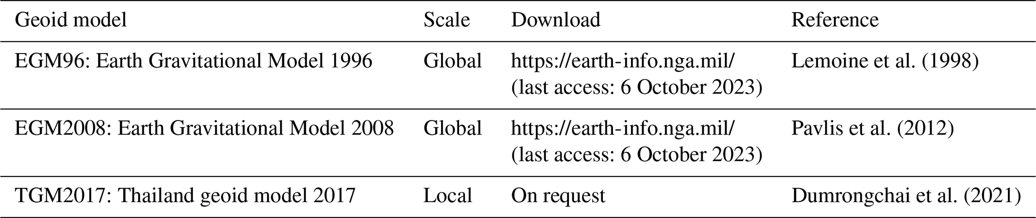
To measure elevations around the Earth, a vertical reference is needed, with mean sea level chosen as the reference. The geoid is the level (equipotential) surface of the Earth's gravity field that best coincides with mean sea level. This surface connects the oceans and extends through the continents. The geoid serves as the reference surface for levelled heights, commonly expressed as “heights above sea level”. In order to compare heights from different data sources, all data have to be re-referenced to the same geoid model. A geoid model is a spatial representation of geoid height, encompassing both global and local scales. This study has collected three geoid models, summarized in Table 1. Thailand has its own local geoid model. The latest one, TGM2017, was released in 2018. This geoid is based on new gravity measurements taken around Thailand and has been shown to better match the expected geoid heights than the EGM2008 model (Dumrongchai et al., 2021). TGM2017 provides the best fit for Thailand; it was chosen as the primary geoid model and all heights were re-referenced to TGM2017.

Table 1 Geoid model datasets.

3.3 Digital elevation models (DEMs)

A digital elevation model (DEM) is a quantitative representation of the Earth's surface elevation. The term “DEM” encompasses both digital terrain models (DTMs) and digital surface models (DSMs). A DSM maps the heights of all features on the surface, such as vegetation and buildings, while a DTM only represents the actual height of the terrain (“bare earth”). Multiple digital elevation models are available; local DEMs are often preferred due to their higher spatial resolution and vertical accuracy (McClean et al., 2020). In this study, we have collected 10 DEM products, as shown in Fig. 2. A summary of these products is presented in Table 2 and detailed statistical analyses are provided in Table A1. The three local DEM products were obtained from the Thai agency, namely, LDD DEM, JICA DEM, and merged LDD-JICA DEM. Additionally, seven global DEMs were collected: ASTER GDEM V3, SRTMv3 DEM, MERIT DEM, FABDEMv1–2 DEM, GLO30 DEM, TanDEM-X, and TanDEM-EDEM.

Table 2 Digital elevation model (DEM).

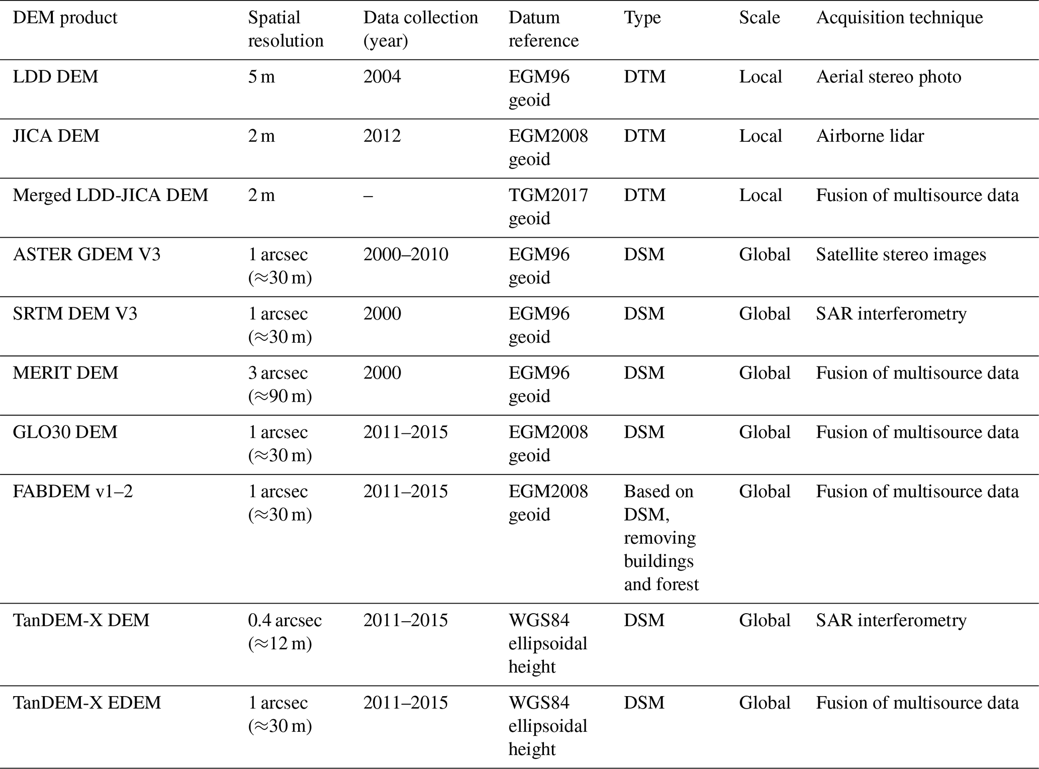
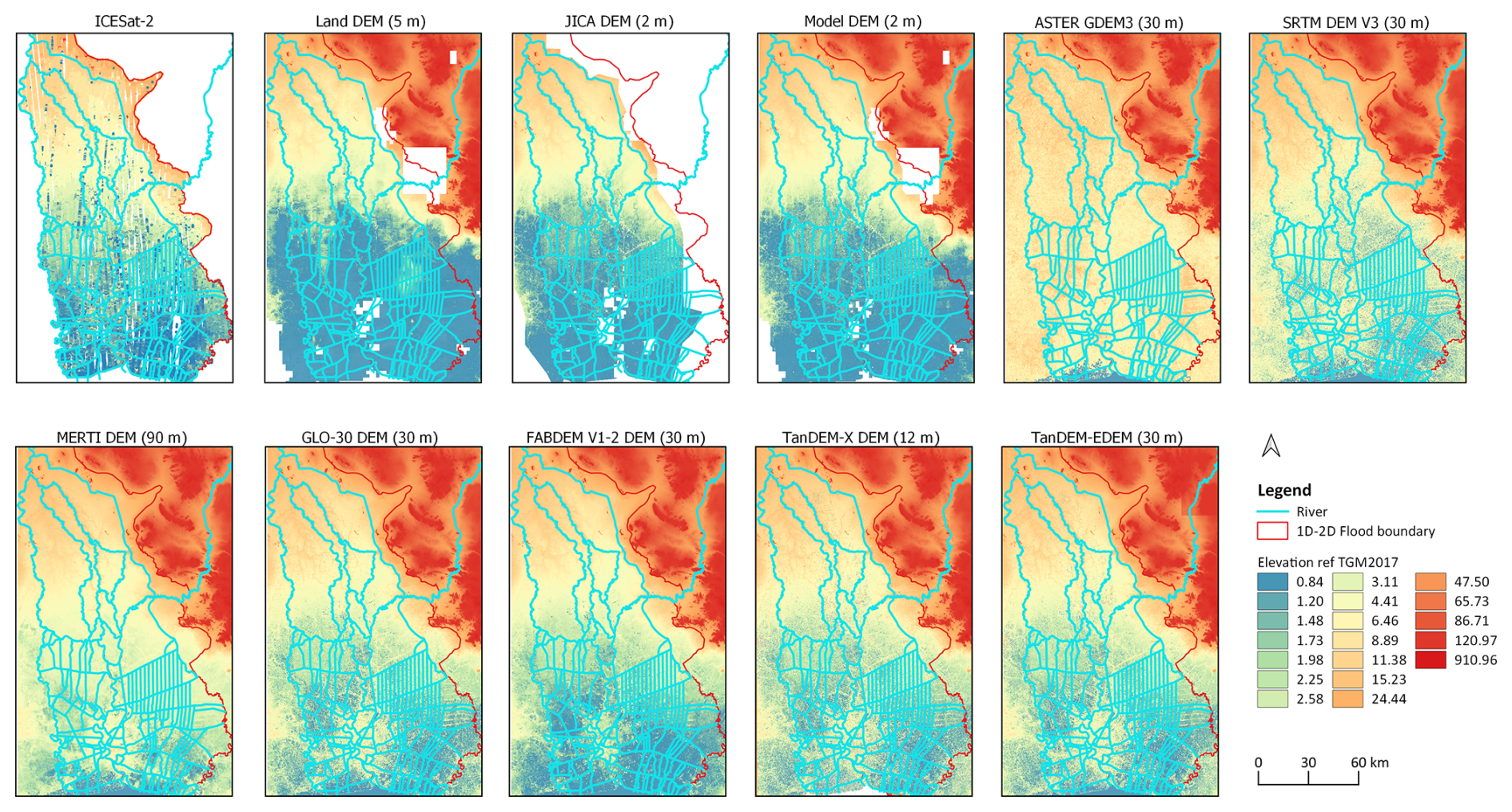
Figure 2 ICESat-2 ATL08 and DEM products: (a) ICESat-2 ATL08 surface elevation, (b) Land Development Department (LDD) DEM, (c) JICA DEM, (d) merged LDD-JICA DEM, (e) ASTER GDEM version 3, (f) SRTM DEM version 3, (g) MERIT DEM, (h) GLO-30 DEM, (i) FABDEM v1.2 DEM, (j) TanDEM-X DEM, (k) TanDEM-EDEM.

3.3.1 LDD DEM

The LDD DEM data are supplied by the Land Development Department (LDD) of Thailand in a grid format, with a resolution of 5 m×5 m. This DEM was generated using photogrammetry, using aerial stereo photo pairs with known scales (Paengwangthong and Sarapirome, 2012). This approach involves deducing distances between points from photos and determining object heights by identifying stereoscopic parallax from multiple pictures and rectifying with ground control points (GCPs) (Sholarin and Awange, 2015). Subsequently, orthorectification and interpolation are used to generate a DEM and mask off buildings and vegetation. Because buildings and vegetation are removed, the LDD DEM approximates a DTM (Sholarin and Awange, 2015).

3.3.2 JICA DEM

The JICA DEM was produced through a collaborative effort between the Royal Irrigation Department (RID) and the Japan International Cooperation Agency (JICA) at a resolution of 2 m×2 m (JICA, 2012). The JICA DEM was generated using airborne laser scanning techniques with lidar (light detection and ranging) aerial technology. The lidar aerial survey employs a pulse laser to measure distances between the target and the sensor; it is applied on a large scale. The distance from the vehicle to the surface can be determined based on the travel time of the laser pulse (Argall and Sica, 2003). The JICA DEM was processed into a DTM, filtering out such features as transportation facilities, buildings, and vegetation from the original data, as described in JICA (2012).

3.3.3 Merged LDD-JICA DEM

The merged LDD-JICA DEM was generated by integrating the LDD and JICA DEMs, as described by Charoensuk et al. (2018). The JICA DEM served as the primary dataset, while the LDD DEM was utilized in areas with gaps within the 1D–2D flood modelling boundary. To incorporate the LDD DEM in the merged LDD-JICA DEM within data gaps, we applied bias correction. The native LDD DEM and JICA DEM datasets were not referenced to the same vertical datum. The processing of the merged LDD-JICA DEM consisted of two primary steps (Fig. A2): (1) re-referencing both LDD DEM and JICA DEM to the TGM2017 reference and (2) calculation of the correlation coefficient between the JICA and LDD DEM for 1000 random points, using linear regression to correct the bias in the LDD DEM, as shown in Fig. A3. Following this, the JICA and LDD DEMs were combined to create the merged LDD-JICA DEM using linear regression. The resulting combined merged LDD-JICA DEM has a resolution of 2 m×2 m.

3.3.4 ASTER GDEM3

The Advanced Spaceborne Thermal Emission and Reflection Radiometer (ASTER GDEM3), serving as a global DEM, was developed by the Ministry of Economy, Trade, and Industry (METI) of Japan in collaboration with the United States National Aeronautics and Space Administration (NASA) and was published on 2019. The footprint of ASTER GDEM spans latitudes from 83° N to 83° S. The study area utilized ASTER GDEM3 (Abrams et al., 2020), which can be downloaded from the associated website: https://gdemdl.aster.jspacesystems.or.jp/ (last access: 12 June 2023). More information is shown in Table 2.

3.3.5 SRTMv3 DEM

The Shuttle Radar Topography Mission (SRTM) DEM, developed by NASA, was a collaborative effort involving the National Geospatial-Intelligence Agency (NGA) and the German and Italian space agencies. It was part of an international project aimed at acquiring radar data, which were used to create the first near-global set of land elevations (Werner, 2001). The DEM was launched in 2000 (Farr et al., 2007) and many improvements have been made since then. The SRTMv3 DEM, the latest version, was used for the study area and can be downloaded from the associated website: https://search.earthdata.nasa.gov/search (last access: 19 September 2023).

3.3.6 MERIT DEM

The Multi-Error-Removed Improved-Terrain (MERIT) DEM, developed by Yamazaki et al. (2017), improves on previous DEMs by systematically removing various error components, such as absolute bias, stripe noise, speckle noise, and tree height bias, from SRTM3 DEM (Farr et al., 2007) and AW3D-30 m DEM (Tadono et al., 2015) and gap-filling with the Viewfinder Panoramas (VFP) DEM (http://viewfinderpanoramas.org/dem3.html, last access: 28 June 2023). The MERIT DEM is a DSM with a resolution of 3 arcsec. It was utilized for the study area and is available for download from the dedicated website: http://hydro.iis.utokyo.ac.jp/~yamadai/MERIT_DEM/index.html/ (last access: 19 June 2023).

3.3.7 GLO30 DEM

The Copernicus DEM, published in 2019 by the European Space Agency (ESA) (CDSE, 2022), represents an upgraded iteration of the WorldDEM. The backbone of the Copernicus WorldDEM is the TanDEM-X mission dataset, yet void filling techniques and integration of other data sources are used to enhance data completeness and accuracy. The Copernicus DEM is provided in three different DSM instances: EEA-10, GLO-30, and GLO-90. For this study, GLO-30 was utilized, offering 1 arcsec resolution. It can be downloaded from the dedicated website: https://spacedata.copernicus.eu/de/collections/copernicus-digital-elevation-model (last access: 23 June 2023).

3.3.8 FABDEMv1–2

The Forest and Building Removed Copernicus Digital Elevation Model (FABDEM) was developed in collaboration between Bristol-based flood modelling company Fathom and the University of Bristol FloodLab. FABDEM V1–0, launched in 2021 (FABDEM V1–0), is derived from the Copernicus GLO-30 (CDSE, 2022) DSM. FABDEM V1–2, released in 2023 (Neal and Hawker, 2023), has a 1 arcsec resolution and is based on a DSM that removes buildings and vegetation. This dataset was employed for the study area and is available for download from https://data.bris.ac.uk/data/dataset/s5hqmjcdj8yo2ibzi9b4-ew3sn (last access: 23 June 2023).

3.3.9 TanDEM-X DEM

TanDEM-X (TerraSAR-X Add-on for Digital Elevation Measurement) is an innovative space borne-radar interferometer based on two TerraSAR-X radar satellites flying in close formation (Krieger et al., 2007). The TanDEM-X mission represents a collaborative effort between the German Aerospace Center (DLR) and AIRBUS (Wessel, 2016), with the aim of generating a globally consistent DEM. TanDEM-X, launched in 2016, is a DSM with resolutions of 0.4, 1, and 3 arcsec. The 3 arcsec TanDEM-X product is readily accessible and can be downloaded directly from https://geoservice.dlr.de/data-assets/ju28hc7pui09.html (last access: 14 September 2023). However, the 0.4 and 1 arcsec products are available from DLR on request. It is important to note that the TanDEM-X product has not undergone full processing to eliminate artefacts, outliers, noisy regions, and data gaps. As a result, its adoption in flood modelling has been limited (McClean et al., 2020). In this study, we employed TanDEM-X with a 0.4 arcsec resolution for our flood modelling purposes.

3.3.10 TanDEM-EDEM

The TanDEM-X Edited Digital Elevation Model (TanDEM-EDEM) is an edited version of the TanDEM-X global model, with a 1 arcsec (≈30 m) pixel resolution, released in 2023 (Wessel, 2016). The main update in TanDEM-EDEM version 1 includes the filling of gaps with suitable alternative DEM data and improved representation of water bodies. The TanDEM-EDEM dataset, which is a DSM, was utilized for the study area and is readily available for download from https://download.geoservice.dlr.de/TDM30_EDEM/ (last access: 27 November 2023). It has a resolution of 30 m.

3.4 ICESat-2 satellite laser altimetry

Ice, Cloud, and Land Elevation Satellite-2 (ICESat-2) is a laser altimetry satellite launched by the US National Aeronautics and Space Administration (NASA) in 2018. As the follow-on satellite of ICESat, ICESat-2 continues elevation measurements of ice sheets, glaciers, sea ice, and various other land features with a 91 d exact repeat orbit. ICESat-2 carries the Advanced Topographic Laser Altimeter System (ATLAS), which works by transmitting 10 000 laser pulses per second using laser light of 532 nm (Neumann et al., 2019). The pulse rate enables the satellite to capture a measurement every 70 cm along the ground track. The pulse divides into six beams, organized into three pairs. Each pair comprises one right-side beam and one left-side beam, which strike the Earth at a distance of 90 m from each other. The distance between each pair is 3.3 km, as depicted in Fig. 1e.

Table 3 ICESat-2 product.

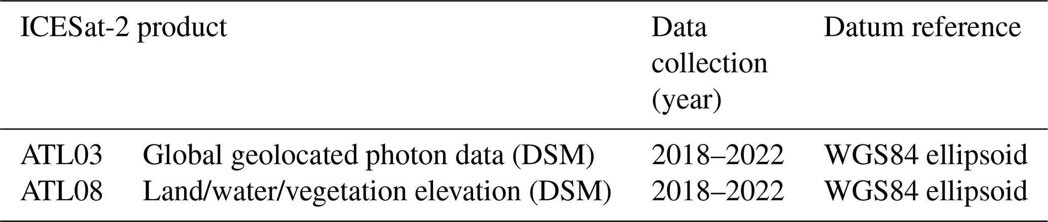
The National Snow and Ice Data Center (NSIDC) portal has developed various products that incorporate photon travel times and locations, determined using the built-in GPS from the ICESat-2 satellite. This mission generates 21 products, as detailed on their website: https://nsidc.org/data/icesat-2/products (last access: 12 June 2023). The two data products used in this study are ATL03 and ATL08, as summarized in Table 3, and the ground track pattern of ICESat-2 in the study area is shown in Fig. 1b. The ICESat-2 data were obtained from the NSIDC website via their data access tool (https://nsidc.org/data/data-access-tool, last access: 12 June 2023).

3.4.1 ATL08

The ATL08 product is derived from ICESat-2 ATL03 data, which provide detailed information on time, latitude, longitude, and height for each photon track. This dense photon dataset enables subsequent analyses and the creation of surface-specific products, such as land ice height and sea ice freeboard (Neumann et al., 2021). The ATL08 product offers estimates of terrain heights, canopy heights, canopy cover, and other descriptive parameters at fine spatial scales in the along-track direction. A fixed segment size of 100 m was chosen to provide continuity of data parameters on the ATL08 data product. Height estimates from ATL08 can be compared with other geodetic data and serve as input for higher-level products like ATL13 (inland water-related heights) and ATL18 (terrain and canopy feature maps) (Neuenschwander et al., 2022). In this study, we used ATL08 land heights from ICESat-2 as the benchmark, against which various DEM products were compared.

3.5 Flood map/surface water extent (SWE) dataset

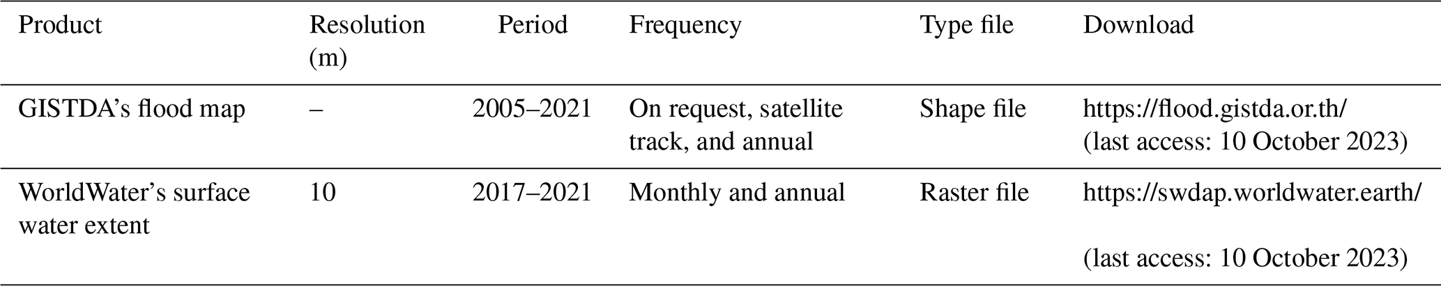
In this study, SWE and flood maps were collected from two sources: surface water extent (SWE) data were collected from the WorldWater project (https://worldwater.earth/, last access: 10 November 2023), funded by the European Space Agency (ESA), and flood map data were collected from the public organization Geo-Informatics and Space Technology Development Agency (GISTDA) in Thailand. The flood map datasets are summarized in Table 4 and presented in Fig. 3.

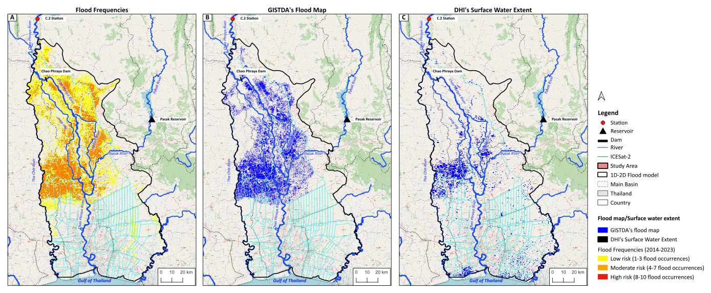
Figure 3 Flood map/surface water extent in study area: (a) flood frequency from HII, (b) GISTDA's flood map in November 2017, (c) WorldWater's SWE in November 2017. © OpenStreetMap contributors 2015. Distributed under the Open Data Commons Open Database License (ODbL) v1.0.

Table 4 Flood map datasets.

3.5.1 WorldWater surface water extent (SWE)

We used SWE products from the WorldWater project, using data from the Sentinel-1 and Sentinel-2 imaging satellites, both integral parts of the ESA Copernicus programme. The Sentinel-1 satellite, launched in 2014, is equipped with a SAR constellation consisting of two polar-orbiting satellites, with objectives on land and ocean monitoring. Sentinel-1 comprises a C-band SAR sensor with a 10 m spatial resolution (Torres et al., 2012). The Sentinel-2 satellites consist of two satellites, namely Sentinel-2A and Sentinel-2B, launched in 2015 and 2017, respectively. The dual-satellite system operates in coordination with a 180° phase difference in the sun-synchronous orbit, supporting both land and ocean monitoring (ESA, 2015). The WorldWater SWE mapping algorithm utilized Sentinel-1 and Sentinel-2 data from 2017 to 2021 to develop a SWE dataset. The details of the Sentinel-1 and Sentinel-2 datasets are accessible from the Copernicus Open Access Hub. This algorithm utilizes a fusion approach (Tottrup et al., 2022), combining optical and radar observations, to provide a more robust delineation of water surfaces. The SWE products provide information on water occurrence, monthly water presence, water seasonality, and maximum and minimum water extent, all accessible on the website: https://swdap.worldwater.earth/ (last access: 10 November 2023). The monthly water presence of the WorldWater SWE in November 2017 is illustrated in Fig. 3c. It is important to note that the WorldWater SWE dataset uses a median composite of all Sentinel-1 and Sentinel-2 acquisitions within a given month to predict monthly surface water presence. Consequently, it does not necessarily reflect the maximum extent of flooding within each month.

3.5.2 GISTDA flood map

GISTDA is a Thai space agency and space research organization that utilizes satellites such as Cosmo-SkyMed, KOMPSAT, LANDSAT-5, RADARSAT-2, and THAICHOTE (Channumsin et al., 2020) to conduct research and development. GISTDA receives observations of the Earth through the use of synthetic-aperture radar (SAR) and optical sensor satellites (Nithirochananont et al., 2010). SAR satellite information is derived from two constellations: RADARSAT and the Advanced Land Observing Satellite (ALOS). RADARSAT comprises two SAR satellites, while ALOS integrates a SAR satellite with an optical satellite. Both RADARSAT and ALOS possess SAR data processing systems. In flooded areas, the Earth's surface appears smooth in the wavelength of the SAR. This smooth surface causes microwaves to reflect in a specular way, resulting in low backscatter values. This characteristic allows for real-time flood imaging and identification. The SAR data undergo processing and image quality enhancement, with elimination of any noise present in the data products (Auynirundronkool et al., 2012).

To generate flood maps from satellite data, GISTDA employed several analysis methods, including supervised classification, visual analysis, and thresholding, which were combined with field images. Subsequently, GISTDA used the boundaries of natural and permanent water sources from the existing database and removed these areas from the flood map. Since 2005, GISTDA has annually published nowcast flood maps and flood occurrence maps on https://flood.gistda.or.th/ (last access: 10 October 2023), which were utilized in this study. The GISTDA flood occurrence map is shown in Fig. 3b.

From 2014 to 2023, HII analysed flood frequency maps from GISTDA. The assessment focused on the frequency of flood occurrences, which were categorized in three levels: low, medium, and high-risk flood frequency. Low-risk flood frequency is defined as 1–3 occurrences within the 10-year span, medium risk as 4–7 occurrences, and high risk as 8–10 occurrences, as depicted in Fig. 3a.

4 Methodology

The workflow used in this study, illustrated in Fig. 4, comprises two primary components. The first component, namely DEM analysis, focuses on evaluating the DEMs (Sect. 3.3), with the ICESat-2 benchmark (Sect. 3.4) as a high-precision reference, which effectively serves as the “ground truth”. The best DEM identified in the DEM analysis is then used as the input to the flood map analysis. The flood map analysis focuses on evaluating flood maps generated by the 1D–2D flood model (Sect. 3.1) against WorldWater SWE and GISTDA flood maps (Sect. 3.5).

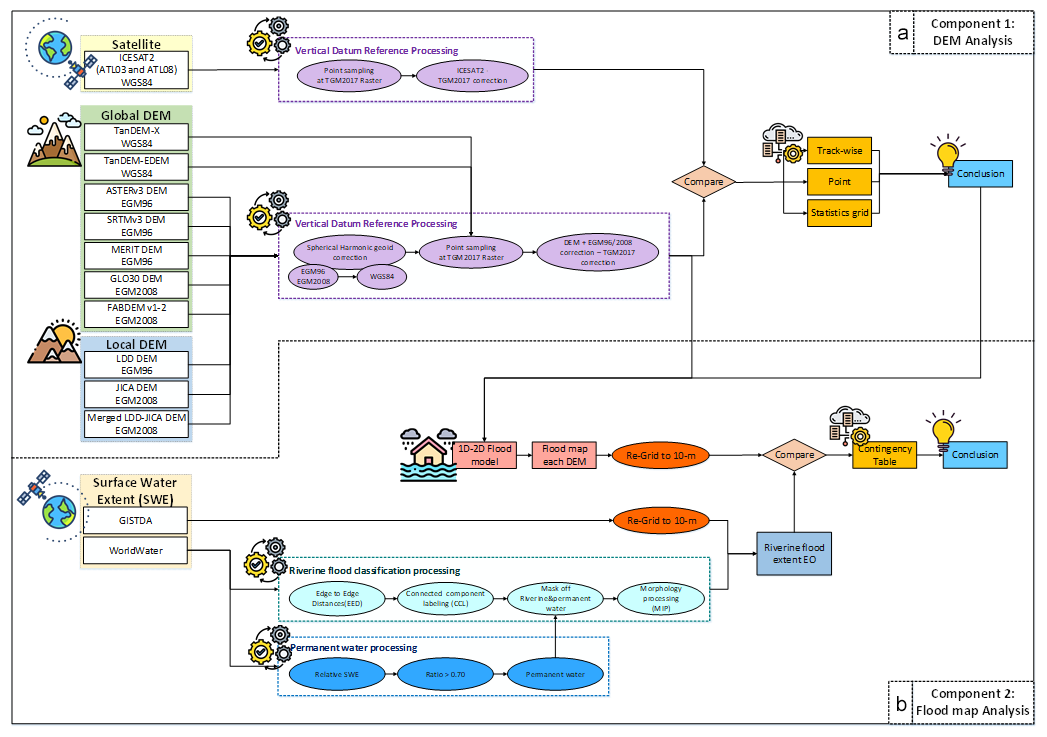
Figure 4 Overall methodology. (a) Component 1: DEM analysis – involves processing ICESat-2 ATL08 data, applying vertical datum referencing, and evaluating DEMs against the ICESat-2 ATL08 benchmark through point, grid, and track-wise comparisons. (b) Component 2: flood map analysis – includes setting up the 1D–2D flood model, performing flood classification, and evaluating flood maps using appropriate methods.

4.1 DEM analysis

The primary objective is to assess the accuracy and reliability of the DEMs by comparing them with elevation data obtained from ICESat-2 using statistical methods. In the study area, ICESat-2 ATL08 data were primarily used for evaluation, while ICESat-2 ATL03 data were employed in complex terrain. Figure 4a illustrates the workflow, involving processing and re-referencing steps. Subsequently, the evaluation of DEMs and ICESat-2 was conducted using statistical methods.

4.1.1 ICESat-2 ATL08 data processing

ATL08 provides estimates of terrain height, canopy height, and canopy cover at fine spatial scales in the along-track direction. For each parameter, terrain surface elevation and canopy heights were provided at a fixed along-track segment size of 100 m (Neuenschwander et al., 2022). The ATL08 dataset comprises a total of 18 land parameters, such as mean terrain height for segment (h_te_mean), mode of terrain height for segment (h_te_mode), number of ground photons in segment (n_te_photins), slope of terrain within segment (terrain_slope), and best fit terrain elevation at the 100 m segment mid-point location (h_te_best_fit). We processed the ATL08 dataset, extracting the latitude and longitude of the photon signals along with the photon heights above the WGS84 ellipsoid. The terrain elevation parameter used for evaluation was h_te_best_fit.

4.1.2 Vertical datum reference processing

To evaluate the DEMs with the ICESat-2 benchmark, it is necessary to use the same vertical datum reference. Vertical datum reference processing was employed to standardize the datum reference. In this study, the vertical datum reference was TGM2017, using Eq. (1) to establish accurate measurements of vertical elevation:

$$\begin{array}{}\text{(1)}& H=h-N,\end{array}$$

where H is orthometric height, h is ellipsoid height, and N is geoid height. Thus,

$$\begin{array}{}\text{(2)}& H_{\mathrm{DEM}\mathrm{ref}\mathrm{TGM}\mathrm{2017}}=h_{\mathrm{DEM}}+N_{\mathrm{DEM}}-N_{\mathrm{TGM}\mathrm{2017}},\end{array}$$

where H_{DEM ref TGM2017} is the DEM referenced to TGM2017, h_DEM represents the original DEM, N_DEM is the geoid reference of the original DEM, and N_TGM2017 is the TGM2017 geoid model.

To obtain DEMs referenced to TGM2017, EGM96 and EGM2008 height corrections were added to the DEM heights, followed by subtracting the TGM2017 geoid corrections, as shown in Eq. (2). The geoid model datasets are shown in Sect. 3.2 for reference. For ICESat-2 elevations referenced to TGM2017, the TGM2017 correction was subtracted from the ICESat-2 elevation data.

4.1.3 Evaluation of DEMs using ICESat-2 ATL08 benchmark

The DEM products were estimated and evaluated using statistical methods, including bias (mean error, ME), mean absolute error (MAE) (Willmott, 2005), mean square error (MSE), root mean square error (RMSE) (Chai and Draxler, 2014), and percentage bias (PBIAS) (Moriasi et al., 2007). The overall purpose of implementing these statistical methods is to evaluate the ICESat-2 ATL08 data paired with the 10 DEM products covering the study area. Subsequently, the performance of the DEMs was systematically compared using statistical indices, defined as follows (Samantaray and Sahoo, 2024):

$$\begin{array}{}\text{(3)}& {\displaystyle }\mathrm{ME}& {\displaystyle }={\displaystyle \frac{\mathrm{1}}{n}}\sum _{i=\mathrm{1}}^n\left(Y_i-{\widehat{Y}}_i\right),\text{(4)}& {\displaystyle }\mathrm{MAE}& {\displaystyle }={\displaystyle \frac{\mathrm{1}}{n}}\sum _{i=\mathrm{1}}^n\left|Y_i-{\widehat{Y}}_i\right|,\text{(5)}& {\displaystyle }\mathrm{MSE}& {\displaystyle }={\displaystyle \frac{\mathrm{1}}{n}}\sum _{i=\mathrm{1}}^n{\left(Y_i-{\widehat{Y}}_i\right)}^{\mathrm{2}},\text{(6)}& {\displaystyle }\mathrm{RMSE}& {\displaystyle }=\sqrt{\sum _{i=\mathrm{1}}^n{\displaystyle \frac{{\left(Y_i-{\widehat{Y}}_i\right)}^{\mathrm{2}}}{n}}},\text{(7)}& {\displaystyle }\mathrm{PBIAS}& {\displaystyle }=\mathrm{100}\times \left[{\displaystyle \frac{\sum _{i=\mathrm{1}}^n\left(Y_i-{\widehat{Y}}_i\right)}{\sum _{i-\mathrm{1}}^n{\widehat{Y}}_i}}\right],\end{array}$$

where ${\widehat{Y}}_i$ represents ICESat-2 ATL08 elevation, Y_i denotes the elevation for each DEM (i.e. LDD DEM, JICA, merged LDD-JICA DEM, ASTER GDEM V3, SRTM DEM, MERIT DEM, FABDEM v1–2 DEM, GLO30 DEM, TanDEM-X, and TanDEM-EDEM), and n is the number of observations. The ideal PBIAS value is 0: positive values indicate that the DEM products tend to overestimate, compared with the ICESat-2 ATL08 benchmark, while negative values indicate a tendency toward underestimation.

We conducted three types of comparisons, as follows.

Point comparison

Point comparison was performed for every segment of the ICESat-2 ATL08 pass over the study area. This approach aimed to provide a quantitative overview of the quality and identify potential discrepancies among the 10 DEMs, in comparison with ICESat-2 ATL08 data (Weifeng et al., 2024), using statistical methods. A total of 954 800 elevation points were extracted from the study area for point-to-point comparison.

Grid comparison

The grid comparison was conducted using a regular square grid over the study area. This comparison provides an overview of the spatial variation of the quality of the DEMs, in comparison with the ICESat-2 ATL08 benchmark. In this study, we employed a 5 km resolution for grid comparison, which involved calculating statistical measures for every segment within each grid cell and displaying the evaluation spatially on a map.

Track-wise comparison

The track-wise comparison was conducted using tracks of ICESat-2 over the study area. The distance between the ICESat-2 points was calculated using UTM x and y coordinates, as shown in Eq. 8. The track-wise comparison represents an overall elevation profile comparison between DEMs and ICESat-2 ATL08 data over the study area:

$$\begin{array}{}\text{(8)}& \mathrm{Distance}=\sqrt{{\left(x_{\mathrm{0}}-x_i\right)}^{\mathrm{2}}+{\left(y_{\mathrm{0}}-y_i\right)}^{\mathrm{2}}},\end{array}$$

where x represents the x coordinates, and y denotes the y coordinates.

4.2 Flood map analysis

The purpose of the flood map analysis is to evaluate the performance of simulated flood maps from the 1D–2D flood model using various DEM products selected from the first component, in comparison with the WorldWater SWE and GISTDA flood maps. This comparative analysis aims to assess the accuracy and effectiveness of the improved flood simulation model.

4.2.1 1D–2D flood modelling setup

The setup of the 1D–2D flood model mirrored the original model, retaining the same parameters, with only the DEM being modified to generate the flood map. The DEM products were selected based on the evaluation of DEMs against the ICESat-2 ATL08 benchmark. Flood maps in the lower CPY basin were simulated using the 1D–2D flood model for the years 2017 and 2021. The flood map simulation results from the 1D–2D flood model present flood extents that occurred during the simulation period and at each daily time step (DHI, 2018). In this study, we employ simulated flood maps generated from a 1D–2D flood model using the merged LDD-JICA DEM and FABDEMv1–2 DEM products and compare them with WorldWater SWE and GISTDA flood maps.

4.2.2 Flood classification processing

The flood map and SWE dataset used for evaluation in this study (Sect. 3.5) had different resolutions, formats, and flood map definitions. To effectively assess the simulated flood map from the 1D–2D flood model, we compared it with the WorldWater SWE and GISTDA flood map. However, it is crucial to employ the same resolution, format, and flood definition. Common types of flooding include flood irrigation, pluvial flash floods, coastal floods, and riverine floods. The 1D–2D flood model only simulates riverine floods, caused by high water levels in the rivers, eventually overflowing onto the neighbouring land due to high river discharge over an extended period. In order to compare the simulated flood map with the satellite EO products, we first have to extract riverine flooding patterns from the surface water extent maps provided by satellite EO. This is done using the following steps.

Permanent water processing

Permanent water bodies should be removed from the satellite EO SWE maps prior to comparison. The GISTDA datasets do not include permanent water bodies. The WorldWater product includes permanent water bodies, which must be removed prior to comparison with simulated flood maps. We use relative water frequency (Yamazaki et al., 2015), which measures the occurrence of surface water within a defined time period. The relative water frequencyf_r of each pixel is defined by Eq. (9) and shown in Fig. A4a:

$$\begin{array}{}\text{(9)}& f_{\mathrm{r}}\left(t\right)={\displaystyle \frac{f_{\mathrm{a}}\left(t\right)}{f_{\mathrm{v}}\left(t\right)}},\end{array}$$

where f_a depicts the frequency of surface water detections during a certain time period for each pixel, and f_v represents the frequency of valid observations during the same period for each pixel.

The relative water frequency ranges between 0.0 and 1.0. The permanent water designation indicates that there was observed water coverage in every single observation of the considered time period, which corresponds to a relative water frequency of 1.0 (Martinis et al., 2022). In many cases, lower thresholds of 0.9, 0.7, and 0.5 were applied (Rao et al., 2018; Yamazaki et al., 2015). The permanent water map for each threshold is illustrated in Fig. A4. In this study, the threshold for relative water frequency is set to 0.7, indicating that a pixel is considered permanent water if it is present in 70 % or more of the valid observations over the specified time period. The output of the permanent water processing is utilized in riverine flood classification processing to remove permanent water from the WorldWater SWE.

Riverine flood classification processing

The WorldWater and GISTDA datasets contain both riverine floods and other inundated areas, caused, for instance, by irrigation or pluvial floods. In order to separate riverine floods in the satellite EO flood maps, we used the following method (Fig. A5).

• Expand the wet area from WorldWater and GISTDA by 200 m using expanding segmentation labels (ESLs) without overlap (van der Walt et al., 2014). The ESL method merges labels in a label image based on the distances between each pixel. Labels that are close by will be merged.

• Subsequently, label each pixel using connected component labelling (CCL) (Rosenfeld and Pfaltz, 1966; AbuBaker et al., 2007). The CCL method is employed to detect connected regions in the binary digital image. The assumption of riverine flood identification is based on the presence of wet connected pixels originating from the river. These are then masked off using ESL, and the riverine flood label is selected.

• Subsequently, the SWE undergoes morphological image processing (MIP) using a closing algorithm (van der Walt et al., 2014). The structuring element, or footprint, passed to the closing algorithm is a Boolean array describing the neighbourhood. We used a disc to create a circular structuring element with a radius of 2, implemented as the footprint. The output provides riverine flood maps, namely WorldWater and GISTDA flood maps, for evaluation with other flood map products.

4.2.3 Flood map evaluation methods

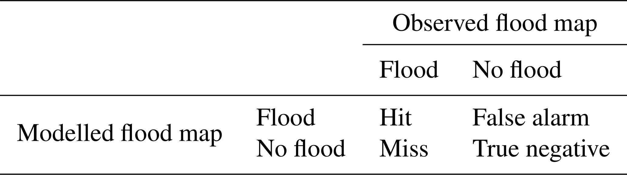
This study evaluates the flood map of the lower CPY River basin using the contingency table (Anon, 1998), comparing flood maps from two different dimensions, shown in Table 5. We evaluated the flood maps produced by the 1D–2D flood model by comparing them with the monthly surface water presence maps from WorldWater and GISTDA for the years 2017 and 2021. We mainly used probability of detection (POD), false alarm ratio (FAR), and critical success index (CSI) (Forecast, 1995) to perform the evaluation. These statistics are based on the number of grid cells or pixels in the study area and are defined as

$$\begin{array}{}\text{(10)}& {\displaystyle }\mathrm{POD}& {\displaystyle }={\displaystyle \frac{\mathrm{Hit}}{\mathrm{Hit}+\mathrm{Miss}}},\text{(11)}& {\displaystyle }\mathrm{FAR}& {\displaystyle }={\displaystyle \frac{\mathrm{False}\mathrm{alarm}}{\mathrm{Hit}+\mathrm{False}\mathrm{alarm}}},\text{(12)}& {\displaystyle }\mathrm{CSI}& {\displaystyle }={\displaystyle \frac{\mathrm{Hit}}{\mathrm{Hit}+\mathrm{False}\mathrm{alarm}+\mathrm{Miss}}},\end{array}$$

where “Hit” represents the number of correctly detected flooded pixels from two different dimensions, “True negative” denotes the number of correctly detected non-flooded or dry areas from two different dimensions, “Miss” indicates the number of floods from dimension 1 that are not detected by dimension 2, and “False alarm” represents the number of floods from dimension 2 that did not occur floods in dimension 1. A perfect score for both POD and CSI is 1, while a value of 0 represents the best score for FAR.

Table 5 Contingency table.

5 Results

5.1 1D–2D flood model calibration results

The 1D river model was calibrated using in situ water surface elevation data for the period 2012 to 2013. The calibration results of the main river in the study area are presented in Charoensuk et al. (2024). The overall performance during the calibration period is generally satisfactory for all main rivers, with an average R² of 0.96, RMSE of 0.30 m, and MSE of 0.90.

The 1D–2D flood model has been calibrated for extreme floods in 2011, as presented in Charoensuk et al. (2018). Normally, flooding in Thailand is influenced by meteorological conditions, river conveyance, and sea level rise. However, the primary cause of the 2011 flood was dyke breaching along the Chao Phraya River, resulting in uncontrollable flood inundation. The simulated flood, when compared with the GISTDA's flood map, satisfactorily corresponds to flood depth, flood propagation direction, and duration.

5.2 Results of DEM evaluation against the ICESat-2 ATL08 benchmark

5.2.1 Point comparison evaluation results

Figure 5 illustrates point comparisons between the statistical metrics of 10 DEM products against the ICESat-2 ATL08 benchmark. As depicted in Fig. 5a, the average ME of the local DEM products was −0.88 m, whereas the average ME of the global DEM products was +1.62 m. The results indicate that local DEM products tend to have negative bias, while global DEM products tend to show positive bias, when compared against the ICESat-2 ATL08 benchmark. This tendency is attributed to the algorithms described in Sect. 3.3, which remove buildings and vegetation from the local DEM products. Moreover, the local DEM products have a finer grid resolution, compared with the global DEM products. The average performance statistics of the local and global DEMs were 1.25 and 2.17 m for MAE, 4.23 and 13.52 m for MSE, and 2.04 and 3.38 m for RMSE, as shown in Fig. 5b–d respectively.

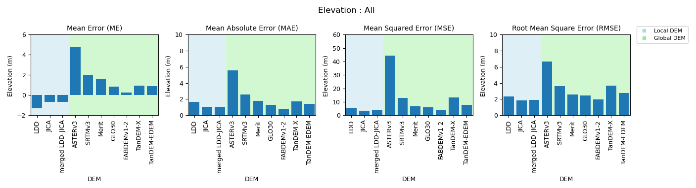
Figure 5 Statistical metrics, comparing 10 DEM products against the ICESat-2 ATL08 benchmark: (a) mean error (ME), (b) mean absolute error (MAE), (c) mean squared error (MSE), (d) root mean square error (RMSE). The resulting averages are computed across the datasets in the study area.

Table 6 presents the statistical results of point comparisons between 10 DEM products, compared with the ICESat-2 ATL08 benchmark, indicating that the accuracy of JICA DEM and FABDEMv1–2 DEM was higher than that of other local and global DEMs. The statistical results of JICA DEM were −0.65, 1.04, 3.51, and 1.87 m and −17.00 % for ME, MAE, MSE, RMSE, and PBIAS, respectively. Specifically, the FABDEMv1–2 DEM showed the highest accuracy, with ME, MAE, MSE, RMSE, and PBIAS values of 0.25, 0.80, 3.79, and 1.95 m and 4.59 %, respectively.

Table 6 Statistical metrics, comparing 10 DEM products against the ICESat-2 benchmark. The resulting averages are computed across the datasets in the study area.

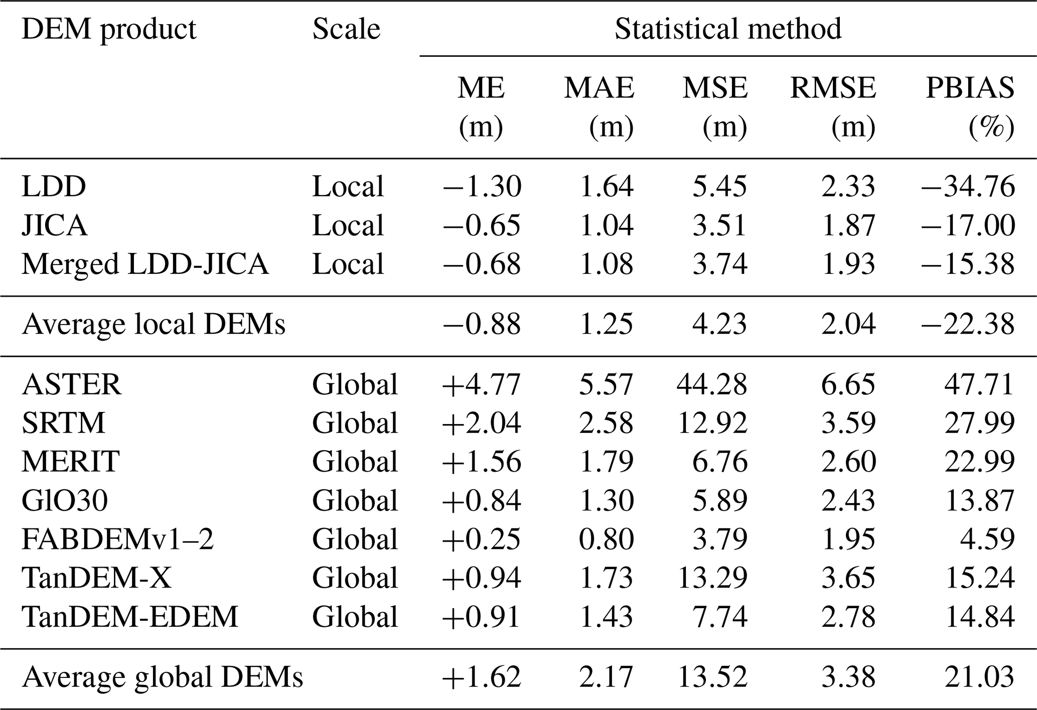
Figure 6 presents the histogram distributions of ME for 10 DEM products relative to the ICESat-2 ATL08 benchmark. The histogram distributions illustrate that the entire curves of local and global DEMs shift towards negative and positive biases, respectively. These shifts indicate that local DEMs, including LDD DEM, JICA DEM, and merged LDD-JICA DEM, exhibit a negative bias in elevation relative to the ICESat-2 ATL08 benchmark, with ME averages of −1.30, −0.65, and −0.68 m, respectively.

Figure 6 Histogram distribution of mean error (ME), comparing 10 DEM products against the ICESat-2 ATL08 benchmark.

Conversely, the shifts observed in the histogram distribution of global DEMs, including ASTERv3 DEM, SRTMv3 DEM, Merit DEM, GLO30 DEM, FABDEMv1–2 DEM, TanDEM-X DEM, and TanDEM-EDEM DEM, indicate a positive bias of the elevation of ICESat-2 ATL08 benchmark. The ME averages for these DEMs were +4.78, +2.03, +1.56, +0.84, +0.25, +0.94, and +0.91 m, respectively. Further details are provided in Figs. A7 and A8, illustrating the mean absolute error (MAE) and mean squared error (MSE), respectively.

5.2.2 Grid comparison evaluation results

Figure 7 displays the ME spatial grid comparison of 10 DEM products against the ICESat-2 ATL08 benchmark, with a resolution of 5 km×5 km. As shown in the figure, the local DEMs indicated, overall, lower values than the benchmark, with LDD DEM showing the lowest ME. In contrast, the overall ME spatial grid comparison of global DEMs was higher than the benchmark and clearly reveals that most global DEMs exhibit poor performance in urban areas. Notably, in the lower middle of the study area lies Bangkok, the capital city of Thailand. However, the FABDEMv1–2 DEM performed better in urban areas, compared with other global DEMs; this can be attributed to the fact that vegetation and buildings are eliminated in this DEM, as described in Sect. 3.3.8 and Dandabathula et al. (2023).

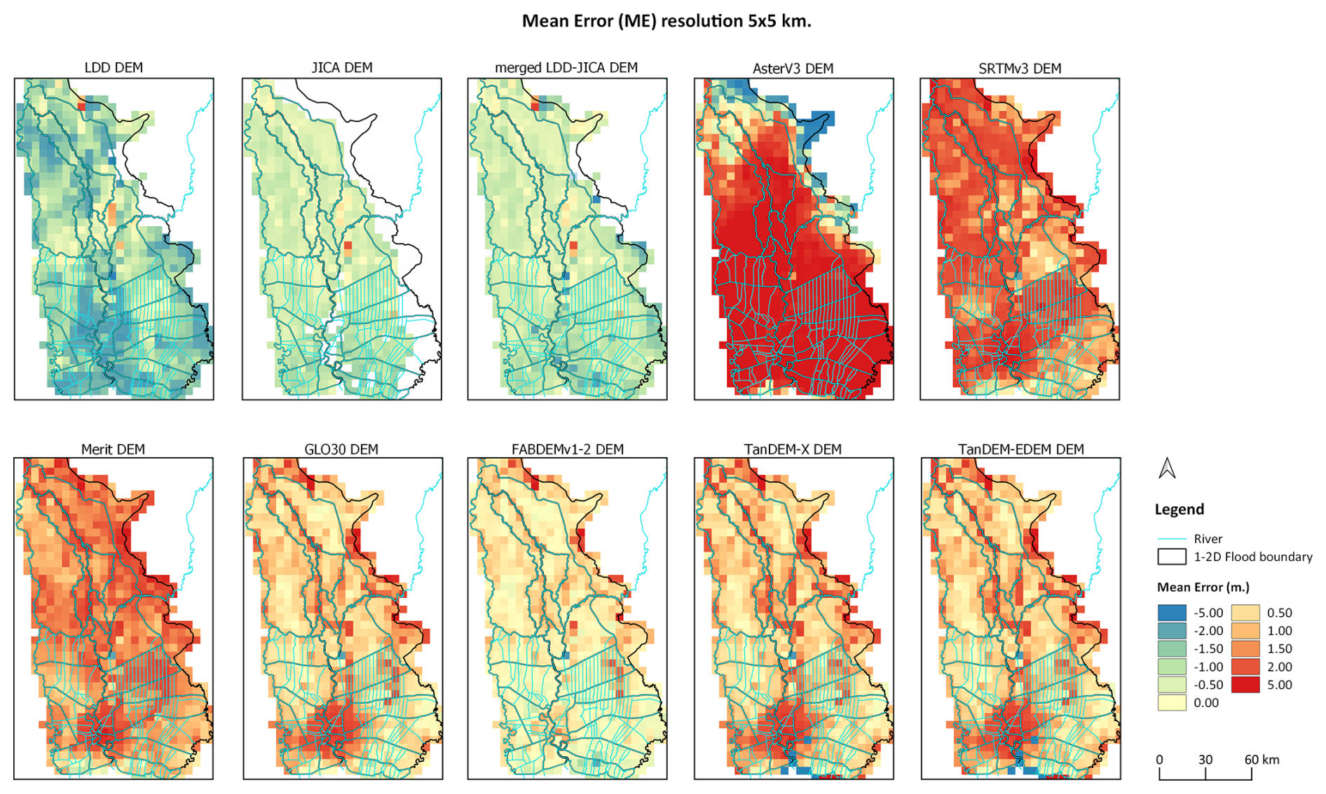
Figure 7 Mean error (ME) spatial grid comparison of 10 DEM products against the ICESat-2 ATL08 benchmark, with a resolution of 5 km×5 km.

5.2.3 Track-wise comparison evaluation results

The track-wise comparison involves comparing the land elevation profile over the study area between the 10 DEM products and the ICESat-2 ATL08 benchmark (see Fig. 8). As shown in Fig. 8, it is evident that the local DEMs exhibit lower land elevation, compared with the ICESat-2 ATL08 benchmark. For most of the tracks, the LDD DEM measures a lower elevation than the benchmark, while the JICA and merged LDD-JICA DEM follow the ICESat-2 ATL08 measurements more closely. This trend is consistent along the majority of the tracks, indicating that the LDD DEM exhibits a negative bias in elevation when compared with ICESat-2. Additionally, both the JICA and merged LDD-JICA DEMs closely track the ICESat-2 measurements for most of the tracks. Moreover, local DEMs show lower elevations in urban areas, in agreement with ICESat-2 ATL08. However, we expect that both local DEMs and ICESat-2 ATL08 still have residual positive bias, compared with the true bare earth elevation in urban areas.

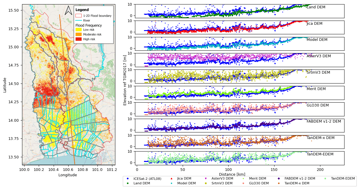
Figure 8 Track-wise comparison of 10 DEM products with ICESat-2 ATL08 benchmark. © OpenStreetMap contributors 2015. Distributed under the Open Data Commons Open Database License (ODbL) v1.0.

Overall, the track-wise comparison of global DEMs shows a higher elevation than the benchmark, especially in urban areas, clearly indicating higher elevations in these urban areas, as illustrated in Fig. 8. In most tracks, ASTERv3 and SRTMv3 DEMs exhibit a notable positive bias and fluctuations, compared with the benchmark. Meanwhile, Merit, GLO30, TanDEM-X, and TanDEM-EDEM DEMs tend to follow a fluctuating pattern and measure slightly higher than the benchmark's track. FABDEMv1–2 closely aligns with the benchmark, indicating its strong performance. More detailed information on the track-wise comparison is provided in Appendix A.

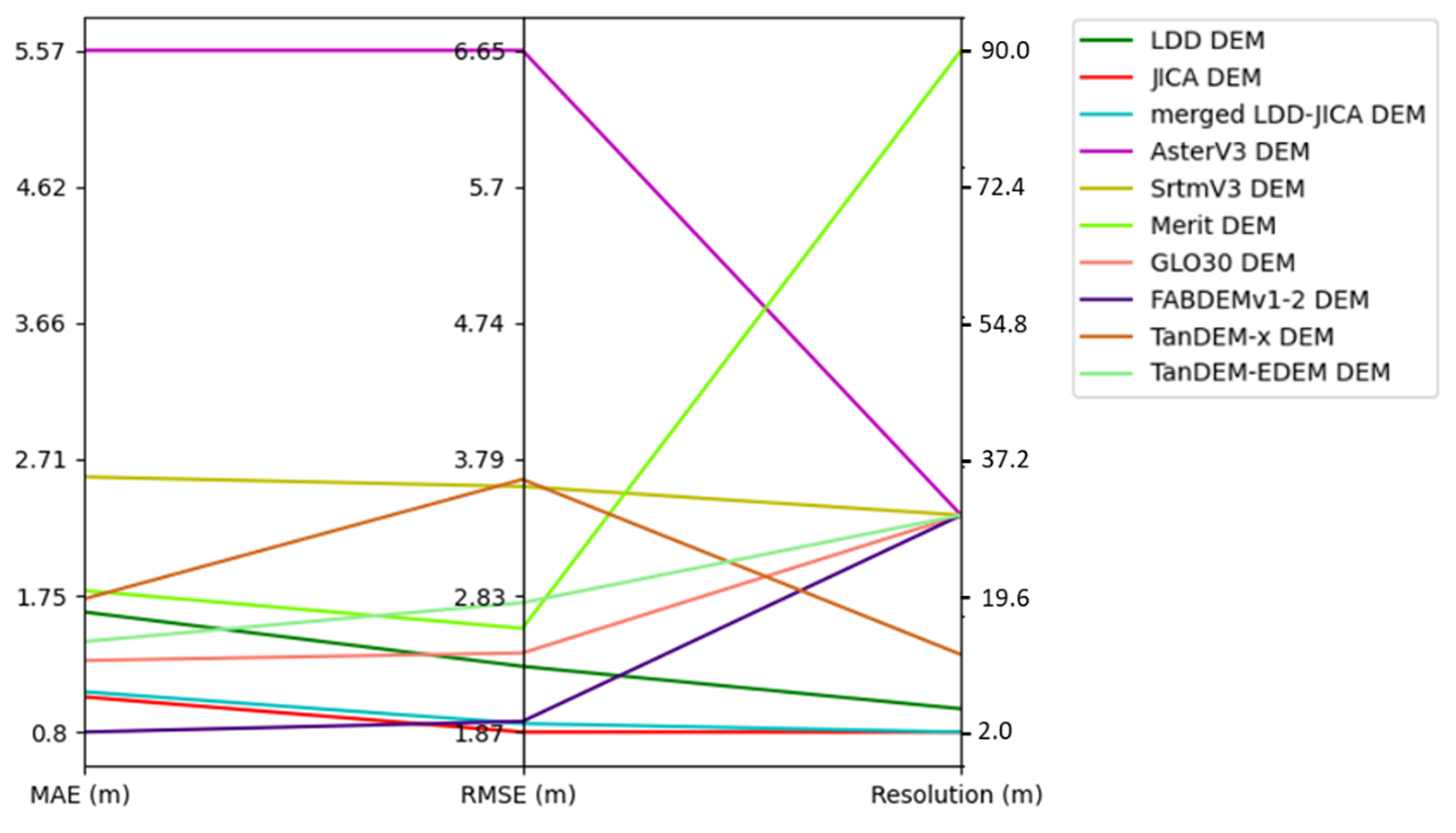
The summary results of the evaluation of the 10 DEM products are presented in the parallel plot shown in Fig. 9, which displays the 10 DEM products along with the results of statistical methods, including MAE, RMSE, and DEM resolution. In the local DEM products, it is notable that LDD DEM exhibits higher error and resolution, compared with the JICA and merged LDD-JICA DEMs. Both the JICA and merged LDD-JICA DEMs demonstrate similar accuracy but the JICA DEM does not cover the entire study area (Fig. 2). Therefore, we utilized the merged LDD-JICA DEM from the local DEM product to implement the 1D–2D flood model. For the global DEM product, the FABDEMv1–2 demonstrates the best performance, compared with other global DEM products. Therefore, we selected the FABDEMv1–2 DEM to implement in the 1D–2D flood modelling, even though its spatial resolution is lower than the TanDEM-X DEM.

Figure 9 Parallel plot of evaluation of 10 DEMs against ICESat-2 ATL08 benchmark.

5.3 Results of evaluation of flood inundation maps

We evaluated simulated flood maps produced using two DEMs: (1) the merged LDD-JICA DEM and (2) the FABDEMv1–2 DEM, as described in Sect. 5.2 from the 1D–2D flood model. The simulated flood map generated by the 1D–2D flood model, referred to as the Model flood map, was evaluated using flood maps from WorldWater and GISTDA for September, October, and November (the flood season) in the years 2017 and 2021. The 1D–2D flood model generated daily simulated flood maps. To ensure accurate comparisons, we selected the dates of satellite passes over the study area, according to WorldWater and GISTDA datasets. These dates were then combined to represent the flood areas that occurred in each month. The results of the flood map evaluation were categorized based on the DEM and compared with the flood maps from WorldWater and GISTDA.

Table 7 Statistical metrics of contingency table, comparing flood map dimensions 1 and 2.

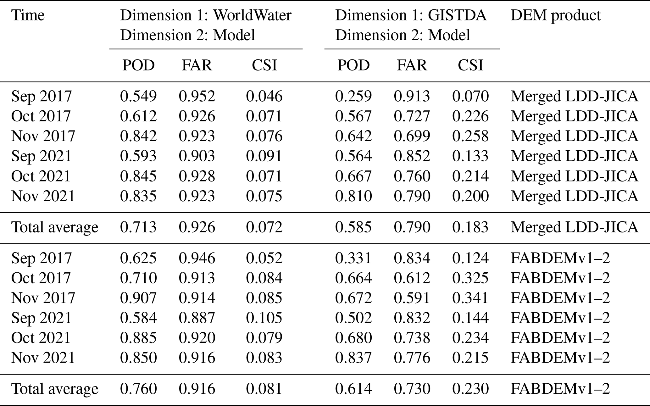
Table 7 provides a comparison of the POD, FAR, and CSI scores for the flood simulation using the merged LDD-JICA DEM, month, and year. Overall, the flood model using the merged LDD-JICA DEM tends to overestimate flooding, particularly in the eastern part of the study area. This overestimation in the eastern part of the study area was attributed to the boundary between the JICA and LDD DEMs in the merged LDD-JICA DEM. The average FAR values of 0.926 and 0.790, along with POD values of 0.713 and 0.585 compared with WorldWater and GISTDA flood maps, respectively, indicate that the Model flood map portrays a larger flood extent while still effectively detecting floods. The average CSI values of 0.072 and 0.183 indicate low model performance and a reflection of the larger flood extent simulation when compared with the flood maps by WorldWater and GISTDA. The overall flood map evaluation based on the FABDEMv1–2 DEM indicates that the Model flood map tends to overestimate, with average FAR values of 0.916 and 0.730 compared with WorldWater and GISTDA flood maps, respectively. Meanwhile, the average CSI values of 0.081 and 0.230 indicate low performance.

Figure 10 shows flood maps and contingency tables for September, October, and November in 2017 and 2021. Figure 10a-1 presents contingency tables comparing WorldWater monthly SWE and Model flood maps based on the merged LDD-JICA DEM in 2017. The results of the evaluation show low CSI values of 0.046, 0.071, and 0.076 for September, October, and November in 2017, respectively, indicating that the Model flood map based on the merged LDD-JICA DEM has low performance. Additionally, the number of false alarms was high, resulting in high FAR values of 0.952, 0.926, and 0.923 for September, October, and November in 2017, respectively. Figure 10b-1 illustrates contingency tables comparing GISTDA and Model flood maps based on the merged LDD-JICA DEM in 2017. The POD values of 0.259, 0.567, and 0.642 are due to the high number of misses, particularly in September in the upper part of the study area. Moreover, the results show more false alarms in the eastern part of the study area, attributed to the combination of LDD and JICA DEMs. The FAR values are 0.913, 0.727, and 0.699 for September, October, and November in 2017, respectively. The CSI values were low in September at 0.070 but increased to 0.226 and 0.258 for October and November, respectively. The detailed statistics are summarized in Table 7.

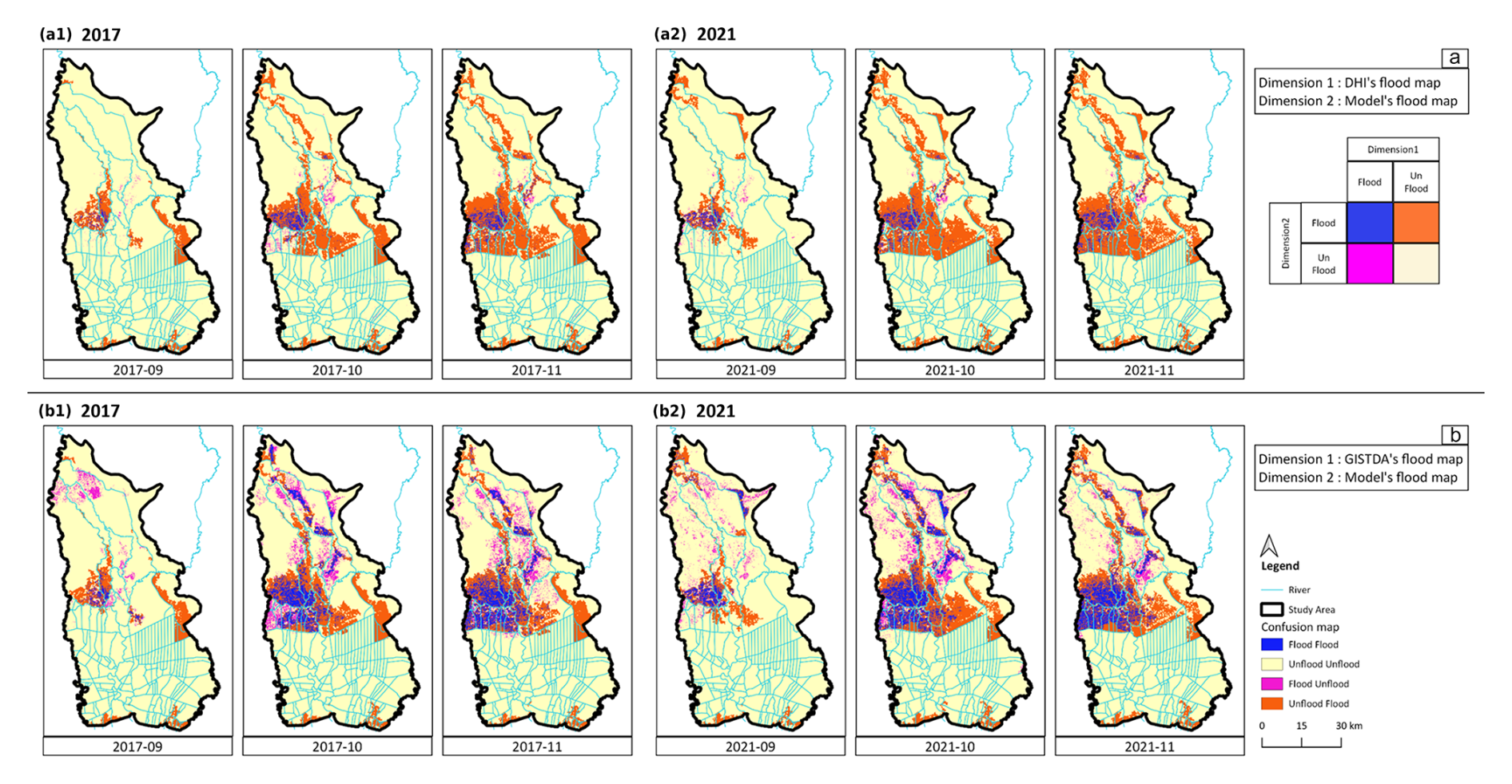
Figure 10 Contingency tables of dimension 1 and dimension 2 flood maps on the spatial map: (a) comparison between WorldWater and Model, based on the merged LDD-JICA DEM, in (a-1) 2017 and (a-2) 2021; (b) comparison between GISTDA and Model, based on the merged LDD-JICA DEM, in (b-1) 2017 and (b-2) 2021.

Figure 10a-2 and b-2 present contingency tables comparing WorldWater and the Model and GISTDA and the Model for each flood-season month in 2021, respectively. The results of flood map evaluation in 2021 followed a similar trend to that of the 2017 flood. In Fig. 10a-2, low CSI values of 0.091, 0.071, and 0.075 are depicted for September, October, and December in 2021, respectively. Additionally, FAR values of 0.903, 0.928, and 0.923, and POD values of 0.593, 0.845, and 0.835, observed for September, October, and November in 2021, respectively, were high. These values suggest that the WorldWater flood map indicates a smaller flood extent, compared with the Model flood map based on the merged LDD-JICA DEM. Figure 10b-2 illustrates an increase in CSI values to 0.133, 0.214, and 0.200 for September, October, and November in 2021, respectively, confirming that the Model flood map based on the merged LDD-JICA DEM fit the GISTDA flood map as well. However, the FAR values were high, at 0.852, 0.760, and 0.790, for September, October, and November in 2021, respectively, indicating that the Model flood map based on the merged LDD-JICA DEM shows overestimated flood extents. Despite this, the POD values of 0.564, 0.667, and 0.810 suggest that the Model flood map based on the merged LDD-JICA DEM can effectively detect GISTDA flood map extents, particularly in October and November.

Figure 11 shows flood maps and contingency tables in 2017 and 2021. Figure 11a-1 illustrates contingency tables comparing WorldWater and Model flood maps based on FABDEMv1–2 DEM for each flood-season month in 2017. The evaluation results clearly indicate that the Model flood tends to overestimate the extent of flooding, as evidenced by FAR values of 0.946, 0.913, and 0.914 and low CSI values of 0.052, 0.084, and 0.085 in September, October, and November in 2017, respectively. However, the POD values were high, with values of 0.625, 0.710, and 0.907 in September, October, and November, respectively, indicating that the Model flood map based on FABDEMv1–2 DEM effectively corresponds to the WorldWater flood map as well, as shown in Table 7. Figure 11b-1 presents contingency tables comparing GISTDA and Model floods for each flood-season month in 2017. Figure 11b-1 confirms the observations made in Fig. 11a-1, indicating that the Model flood map tends to overestimate the extent of flooding, compared with the GISTDA flood map. However, the FAR values decrease slightly, to 0.834, 0.612, and 0.591, and the POD values decrease, to 0.331, 0.664, and 0.672, in September, October, and November in 2017, respectively. The decrease in POD is attributed to a higher number of misses in the upper part of the study area, suggesting that the GISTDA flood map depicts more flooding than the Model flood map based on the FABDEMv1–2 DEM. Conversely, the CSI improved to 0.124, 0.325, and 0.341 in September, October, and November in 2017, respectively, indicating that the model results are more accurate when compared with the GISTDA flood map. Additionally, the figure illustrates that the GISTDA flood map shows a greater extent of flooding, compared with the WorldWater flood map.

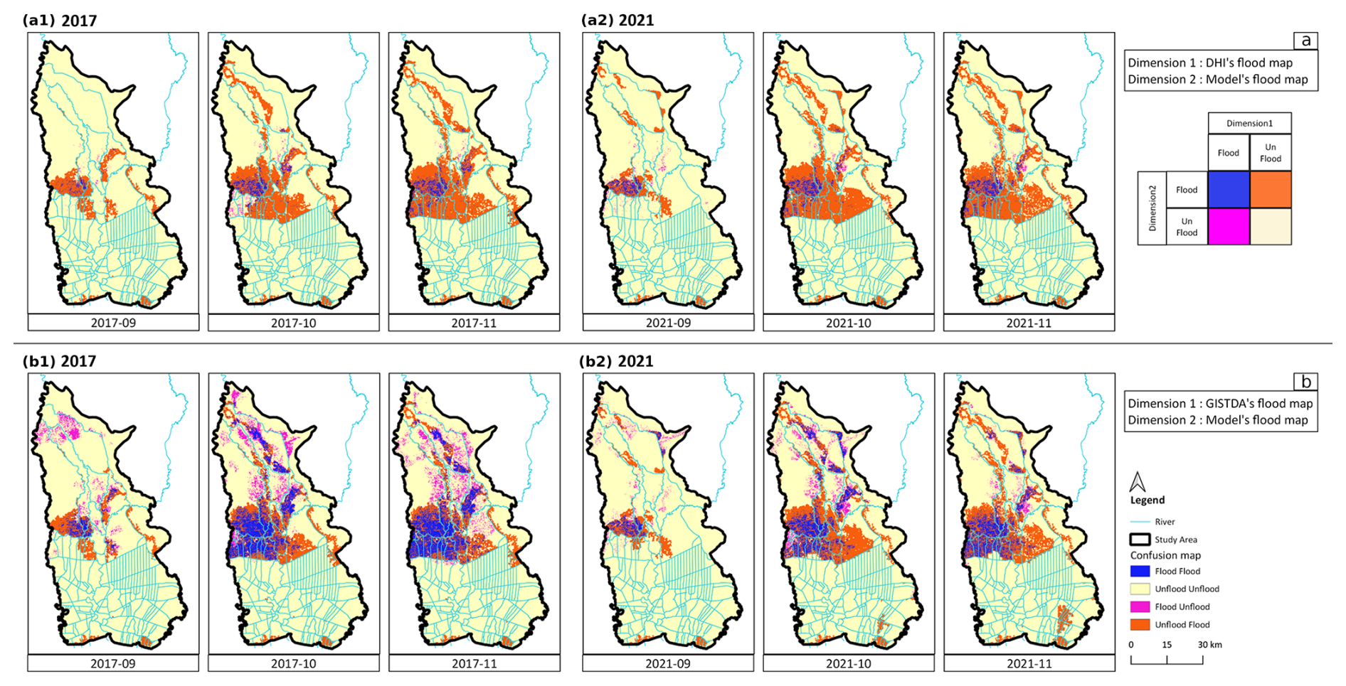
Figure 11 Contingency tables of dimension 1 and dimension 2 flood maps on the spatial map: (a) comparison between WorldWater and Model, based on the FABDEMv1–2 DEM, in (a-1) 2017 and (a-2) 2021; (b) comparison between GISTDA and Model, based on the FABDEMv1–2 DEM, in (b-1) 2017 and (b-2) 2021.

Figure 11a-2 and b-2 depict contingency tables comparing WorldWater and the Model and GISTDA and the Model for each flood-season month in 2021, respectively. The Model flood map based on the FABDEMv1–2 DEM exhibits an overestimation of flooding, which is particularly noticeable in the eastern part of the study area. Figure 11a-2 illustrates high FAR values, of 0.887, 0.920, and 0.916, that indicate that there are more false alarms in September, October, and November, respectively. The POD was high, with values of 0.584, 0.885, and 0.850, and there were low CSI values, of 0.105, 0.079, and 0.083, in September, October, and November in 2021, respectively. This figure illustrates that the Model and the WorldWater flood map indicate more and less flooding, respectively. Figure 11b-2 reveals more misses in the upper part of the study area, resulting in a decrease in the POD values to 0.502, 0.680, and 0.837, compared with Fig. 11a-2. Despite this, the FAR values remain high, at 0.832, 0.738, and 0.776; this is particularly notable in the eastern part of the study area. However, the Model flood map effectively corresponds to the GISTDA flood map as well. The CSI values of 0.144, 0.234, and 0.215 for September, October, and November in 2021, respectively, indicate that the Model flood map exhibits improved accuracy in comparison with the GISTDA flood map.

The overall assessment of the Model flood map, based on both the merged LDD-JICA and FABDEMv1–2 DEMs, indicates an overestimation of flood extent, compared with both the WorldWater and GISTDA flood maps. When comparing the model flood map based on the merged LDD-JICA and FABDEMv1–2 DEMs with each of the WorldWater and GISTDA flood maps, the results consistently indicate a slight improvement in performance for the Model flood map based on FABDEMv1–2. The CSI of the Model flood map based on FABDEMv1–2 increases by 0.010 and 0.047, compared with the Model flood map based on the merged LDD-JICA DEM for the WorldWater and GISTDA flood maps, respectively. Additionally, the FAR is reduced by approximately 0.010 and 0.060 for the WorldWater and GISTDA flood maps, respectively. Although the study used flood classification processing to extract riverine flood maps from the SWE map for comparison, there are still limitations. Continuous improvements in the flood classification process are necessary. The study results show that the overall assessment of flood simulation based on the FABDEMv1–2 DEM reveals a slight improvement of 13.55 %–25.56 % in terms of the CSI, compared with flood simulation based on the merged LDD-JICA DEM. However, the DEM is one factor contributing to improved performance; many other factors still require further improvement.

Figure 12 illustrates the overall performance of the Model flood map, based on both the merged LDD-JICA and FABDEMv1–2 DEMs. The results are presented in three box plots, corresponding to the evaluation metrics: POD, FAR, and CSI. FABDEMv1–2 exhibits a slightly higher median POD than the merged LDD-JICA, indicating a better ability to correctly detect flood events. The interquartile range (IQR) for the merged LDD-JICA is wider, suggesting greater variability in detection performance, compared with FABDEMv1–2, which shows more consistent POD values. Both DEMs show relatively high FAR values, with the merged LDD-JICA having a slightly higher median FAR, indicating that it generates more false alarms. FABDEMv1–2 has a smaller IQR, reflecting more consistent performance in minimizing false alarms, compared with the merged LDD-JICA. Additionally, FABDEMv1–2 demonstrates a significantly higher median CSI than the merged LDD-JICA, reflecting superior overall performance in balancing correct detections and false alarms. The narrower IQR for FABDEMv1–2 suggests more consistent performance, while the merged LDD-JICA shows greater variability in CSI values.

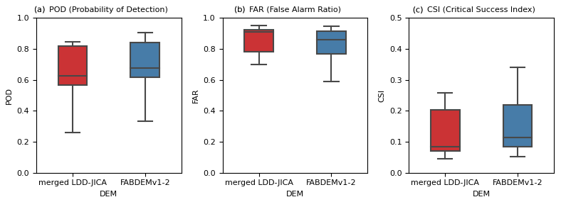
Figure 12 Box plots illustrating the performance of the flood model based on the merged LDD-JICA and FABDEMv1–2 DEMs across three statistical metrics: (a) probability of detection (POD), (b) false alarm ratio (FAR), (c) critical success index (CSI).

6 Discussion

6.1 Overall result of DEM analysis workflow

The result of the DEM analysis shows that ICESat-2 ATL08 data offer a unique advantage in verifying DEM accuracy (Carabajal and Boy, 2020). The overall precision of DEM products was evaluated using the ICESat-2 ATL08 benchmark, showing that the JICA and FAMDEMv1–2 DEMs were significantly better than the local and global DEM products, in terms of average RMSE, with values of 1.87 and 1.95 m, respectively (Fig. 5 and Table 6) in point comparisons. The merged LDD-JICA DEM showed a slight difference of 0.06 m in average RMSE, compared with the JICA DEM. This variance is primarily attributed to the combination of LDD and JICA DEMs, with the JICA DEM chosen as the primary DEM. However, it is noteworthy that the local DEM product exhibited a negative average bias (ME) ranging from −1.30 to −0.65 m, indicating that the elevation of local DEM products is lower than the benchmark. Another study conducted in Spain, which verified airborne lidar data with ICESat-2 ATL08, also reported a negative bias, with average ME values of −0.48 m (Zhu et al., 2022). Conversely, the average ME of the global DEM products yielded positive values ranging from 0.25 to 4.77 m, indicating that the global DEM products overestimate the benchmark. This result has been previously confirmed in such studies as ASTERv3 (Weifeng et al., 2024), STRMv3, and TanDEM-X (Liu et al., 2020). The ASTERv3 DEM showed the lowest overall accuracy, with an average RMSE of 6.65 m. This is in line with other areas, such as the Qinghai–Tibet Plateau, where the RMSE reached 11.47 m (Weifeng et al., 2024). The TanDEM-EDEM is an updated version of the TanDEM-X, which can reduce the error value from 3.65 to 2.78 m in terms of average RMSE.

Figures 7, A10, and A11 illustrate the spatial grid comparison of 10 DEM products against the ICESat-2 ATL08 benchmark, with a resolution of 5 km×5 km for ME, MAE, and RMSE, respectively. The results clearly reveal that the global DEM tends to overestimate, particularly when compared with the ASTERv3 DEM. As shown in the figures, the error of the global DEM clearly clusters in urban areas, except for the FABDEMv1–2, which employs an algorithm to remove building discrepancies, as discussed in Sect. 3.3.8. Although ICESat-2 ATL08 is capable of measuring land elevation very accurately, some urban areas still exhibit positive bias, particularly in dense high-rise areas (Liu et al., 2020), as shown in Fig. 8. This suggests that the DEM analysis workflow can effectively utilize ICESat-2 ATL08 data for evaluation. In certain areas, the incorporation of ATL03 data may be necessary to enhance the evaluation process.

Despite the high spatial resolution of the local DEM (merged LDD-JICA DEM), which is derived from airborne lidar and expected to be highly accurate, the results of this study demonstrate that the global DEM (FABDEMv1–2) can surpass it in specific ICESat-2-based evaluation metrics. Although this finding may appear counterintuitive, it is attributable to several underlying factors that influence DEM performance and consistency.

6.1.1 ICESat-2 ATL08 benchmark

The ICESat-2 ATL08 dataset is derived from ICESat-2 ATL03 photon cloud data through a sequence of processing steps designed to extract accurate land surface elevation and canopy height information. The algorithm comprises several key stages, including noise filtering, surface detection, top-of-canopy identification, photon classification, photon label refinement, canopy height estimation, and link scale for the data product as depicted (Neuenschwander et al., 2021). Notably, the algorithm is optimized to produce smoothed land surface elevation estimates over fixed segment lengths of 100 m. This smoothing inherently aligns better with the spatial resolution of coarser global DEMs. Consequently, global DEMs – such as FABDEMv1–2 – tend to yield terrain representations that are more consistent with the footprint-averaged elevations derived from ATL08.

6.1.2 Quality of DEMs

The accuracy of local DEMs is highly dependent on data acquisition techniques, the acquisition time of the data, and post-processing workflows. Errors can arise from incomplete ground point classification, outdated surveys, or inconsistencies in vertical datum alignment. In the case of the merged LDD-JICA DEM, multiple datasets were combined – some of which were collected long ago (Sect. 3.3) – potentially introducing temporal inconsistencies. Although the JICA DEM component is considered a reliable source, the merging process and age of the data may reduce overall accuracy. In contrast, the ICESat-2 ATL08 dataset benefits from continuous updates, offering more current elevation observations. This is particularly relevant in rapidly evolving urban areas such as Bangkok, where frequent land-use changes can quickly render older DEMs obsolete.

6.2 Overall result of flood map analysis workflow

The flood classification process aims to classify flood types from the SWE map. This method is based on various assumptions and simplifications. The validity of the approach is hard to evaluate, given the lack of ground-truth flood extent observations. However, it is evident that, in this study area, surface water extent is due not only to riverine flooding but also to various other flooding mechanisms, such as irrigation and pluvial flooding.

The Model flood map, based on both Model and FABDEMv1–2 DEMs, tends to overestimate flood extent, compared with the classified flood maps derived from SWE data provided by the GISTDA and WorldWater projects. Additionally, the flood map based solely on FABDEMv1–2 performs slightly better than the one based on the merged LDD-JICA DEM, with an improvement of approximately 13.55 %–25.56 %, according to the CSI. The overestimation of flood inundation from the flood model occurs predominantly in the eastern part of the CPY River, indicating a clear need to improve the 1D–2D flood model. Although this study has incorporated high-quality DEM data, implemented in the 1D–2D flood model, there are still many factors affecting flood map generation. For instance, the 1D–2D flood model, developed long ago (Sect. 3.1), needs to be updated and recalibrated, due to continuous developments in water management plans, such as the Ayutthaya Bypass Channel (JICA, 2018) and ongoing land-use changes in the lower CPY basin (Visessri and Ekkawatpanit, 2020), which impact flood map simulations.

The results of the flood map comparisons demonstrate that the CSI value is relatively better when compared with GISTDA but lower when compared with WorldWater. It is observed that the overall WorldWater flood map shows relatively low flooding compared with the GISTDA flood map. This is due to fundamental differences in the mapping approaches, with WorldWater aiming to provide long-time series of the typical distribution and persistence of monthly surface water presence, whereas GISTDA is targeting real-time maps, showing the extent of flooding at a specific moment in time. Additionally, WorldWater uses only Sentinel-1 and Sentinel-2 data, whereas GISTDA combines data from multiple other satellites, as described in Sect. 3.5. This can be further verified for accuracy with additional information from news sources and by cross-referencing with ICESat-2 ATL13 data, extracted from ICESat-2 ATL03 (inland water surface heights), in main rivers (Coppo Frias et al., 2023; Dandabathula and Srinivasa Rao, 2020). This suggests that the flood analysis workflow can effectively verify the performance of flood simulation using satellite data. Although the flood simulation results in this study meet acceptable standards and are sufficiently reliable for practical applications, the SWE data were generated using different algorithms and satellite sources, resulting in variations in the datasets. These observed datasets were subsequently compared with simulated flood maps derived from various DEM products.

6.3 Advantages and limitations

This study proposes to enhance the performance of 1D–2D flood models using satellite laser altimetry and multi-mission surface water extent maps from EO data. The proposed workflows, encompassing comprehensive DEM analysis and flood map analysis, are designed to be adaptable, scalable, and standardized for the development of 1D–2D flood models. These workflows enable their application across diverse spatial domains, ranging from local to national scales, and can be readily tailored to address flood management challenges in other regions or countries.

Furthermore, the increasing availability of EO data has proven highly effective in improving the accuracy of 1D–2D flood models, particularly in calibration and validation processes. ICESat-2, with its high data precision and 91 d exact repeat orbit, serves as a robust benchmark for evaluating DEM products. Its near-real-time capability is particularly beneficial in areas undergoing rapid land-use changes. Freely available global DEM products, developed using advanced EO techniques, provide high-resolution and high-quality elevation data essential for accurate modelling.

Datasets such as WorldWater's SWE maps and GISTDA's flood maps are valuable resources for assessing the accuracy and reliability of simulated flood maps. By comparing observed flood extents with model outputs, these datasets help identify discrepancies, refine model parameters, and enhance the performance of flood models. This iterative process facilitates the development of more reliable and accurate tools for flood forecasting and management.

Despite these advantages, EO data are not without limitations. For instance, ICESat-2 offers an elevation accuracy of approximately 0.70 m (Neuenschwander et al., 2021; Carabajal and Boy, 2020). However, delays or gaps in EO data acquisition, as discussed in Sects 3.4 and 3.5, can affect the evaluation of simulated flood maps. Furthermore, while the best available DEMs were selected for this study, elevation inaccuracies in certain areas may still compromise the precision of flood inundation maps. Periodic updates to the data, as explained in Sect. 6.2, are necessary to address these limitations and maintain modelling accuracy.

6.4 Future applications

The workflows developed in this study represent a significant advancement in upgrading 1D–2D flood models by integrating satellite laser altimetry and multi-mission satellite surface water extent (SWE) maps. These workflows not only enhance the accuracy and reliability of flood inundation simulations but also offer scalable solutions for improving flood forecasting systems across multiple regions. Their success in the Chao Phraya River Basin sets the foundation for expanding these methodologies to other regions of Thailand, including the eastern (Finn et al., 2018), northeastern (Thanathanphon et al., 2014), southern, and western regions. These regions will benefit from improved model calibration, validation, and more accurate flood forecasts, thereby supporting better decision-making for flood mitigation, response, and water resource management.

Moreover, satellite technology offers new opportunities for measuring water surface elevation (WSE), such as ICESat-2 ATL13 (Jasinski et al., 2023), Surface Water and Ocean Topography (SWOT) (Biancamaria et al., 2016), CryoSat-2 (Kittel et al., 2021; Shen et al., 2020), Jason-2, and Envisat (Okeowo et al., 2017). These technologies enhance calibration, validation, error diagnosis, and monitoring of main river systems, especially in areas with limited ground-based instrumentation.

On a broader scale, the workflows could be adapted for use in other countries, particularly in regions facing similar challenges related to data scarcity, terrain complexity, and high flood risk. The integration of satellite EO data, combined with local hydrological models, could provide valuable insights for flood-prone regions across southeast Asia and beyond, contributing to global efforts in disaster risk reduction and climate resilience.

7 Conclusions

The present study enhanced the performance of 1D–2D flood models using satellite laser altimetry and multi-mission surface water extent maps from Earth observation (EO) data. We demonstrated two workflows in the lower CPY basin.

• DEM analysis workflow. This involved evaluating DEM accuracy using satellite laser altimetry data from ICESat-2 ATL08 before integrating the DEM products into the flood model. The assessment aimed to assess the overall performance of DEM products through vertical, spatial, track-wise analysis, and statistics measures to select the most suitable DEM for the study area. Furthermore, this workflow is transferable to other study areas, providing a method to reduce uncertainty before developing flood models. The results show that the merged LDD-JICA and FABDEMv1–2 DEMs are highly suitable in the study area, with RMSE values of 1.93 and 1.95 m, respectively.

• Flood map analysis workflow. This workflow encompassed riverine flood classification and the evaluation of simulated flood maps generated by the 1D–2D flood model using multi-mission satellite SWE maps. While the flood classification algorithm still presents challenges, it is important to recognize that SWE maps derived from satellite EO cannot be directly compared with the output of flood models without further processing. The flood map evaluation method facilitated the assessment of flood simulation accuracy against satellite SWE maps, employing statistical and spatial analyses. These evaluations contribute significantly to the calibration and validation of flood maps derived from the 1D–2D flood model. The results indicate that simulated flood maps based on FABDEMv1–2 DEM can improve the performance of the 1D–2D flood model by 13.55 % to 25.56 %, as determined by the CSI, when compared with simulated flood maps based on the merged LDD-JICA DEM.

Integrating these workflows will enhance the efficiency of the 1D–2D flood model and showcase the potential of utilizing EO satellite data to enhance flood modelling capabilities for operational flood forecasting in Thailand and elsewhere.

Appendix A

Table A1 Descriptive statistics of 10 different DEM products.

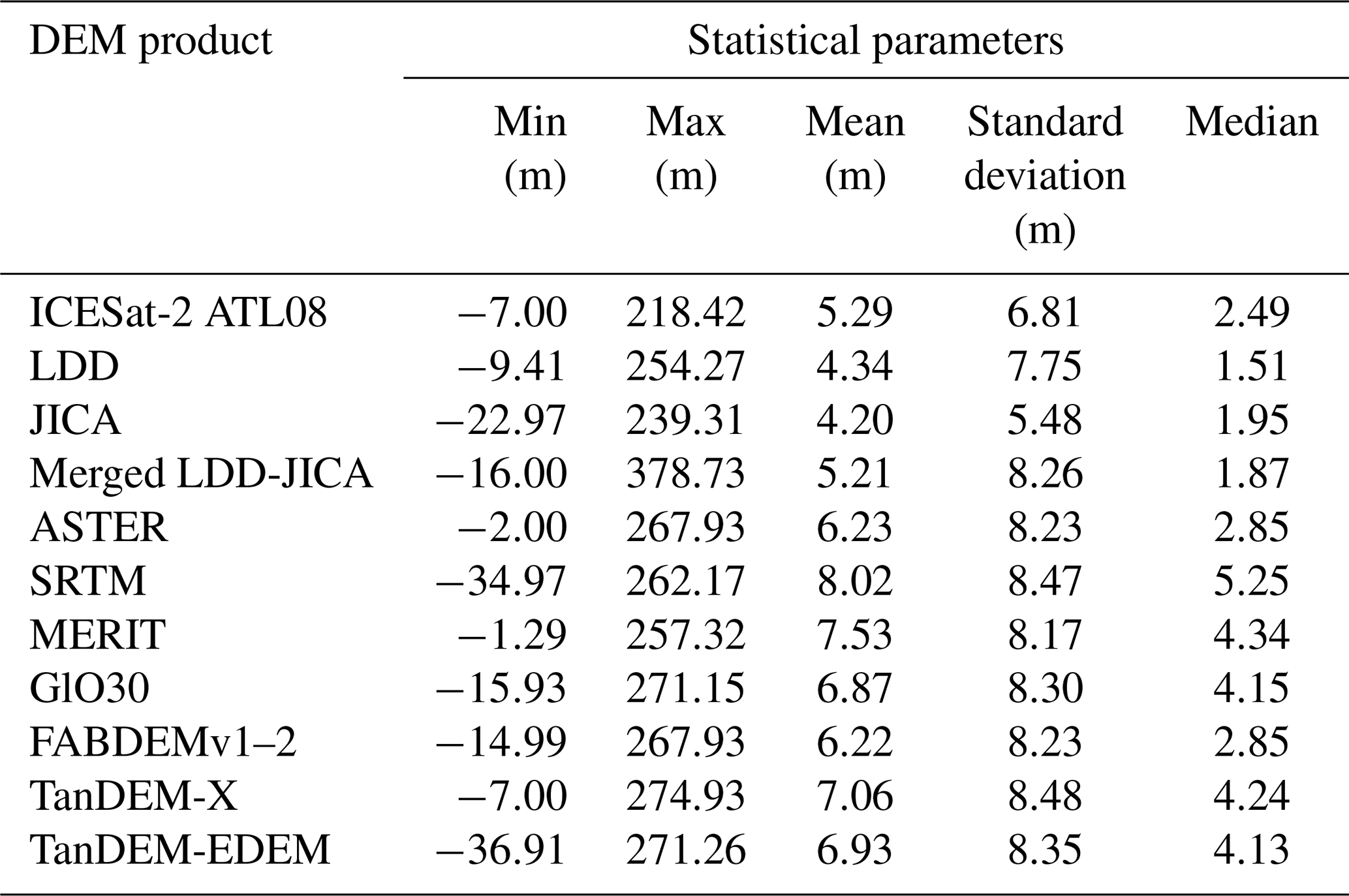
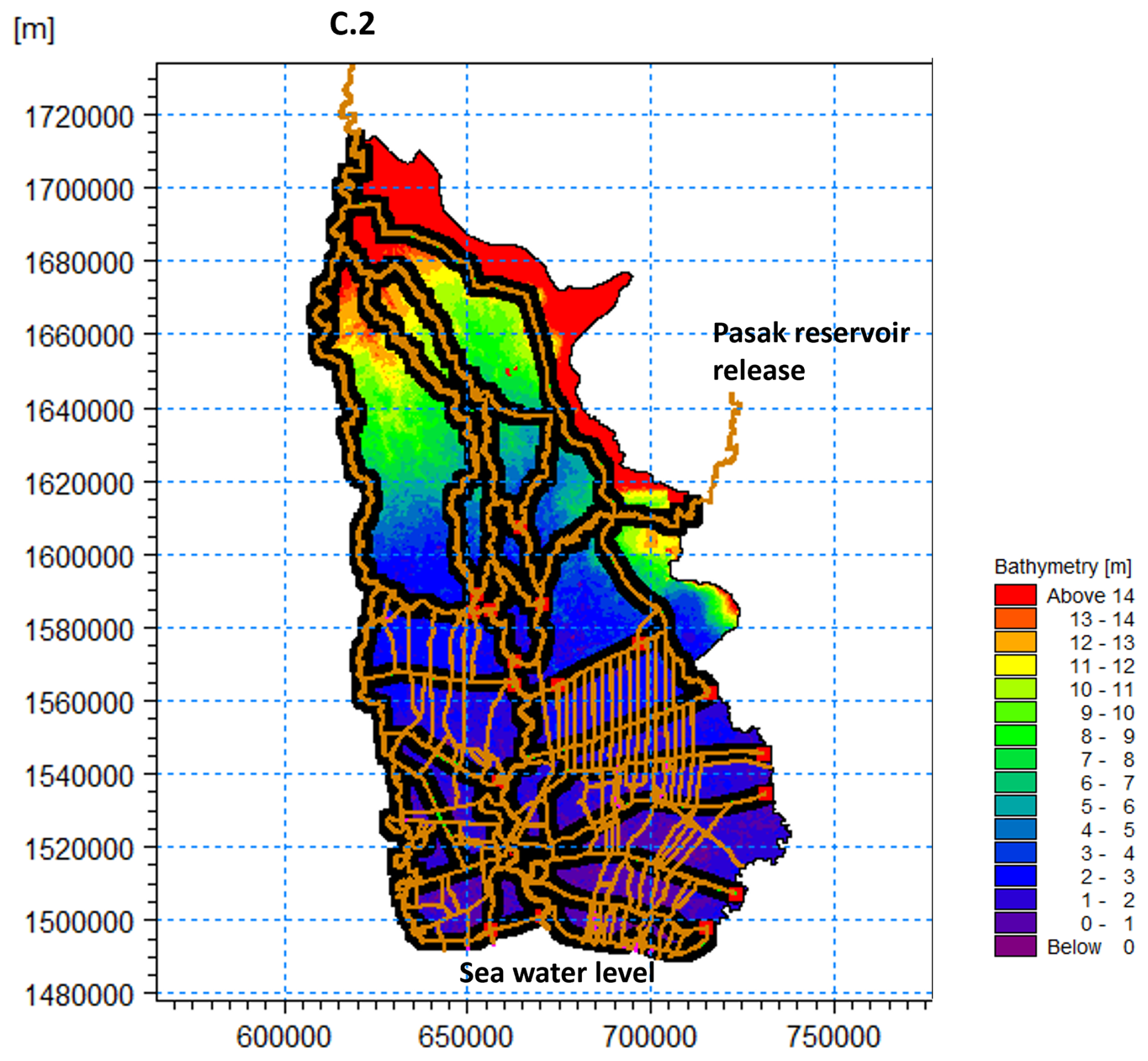
Figure A1 1D–2D flood model.

Figure A2 Merged LDD-JICA DEM workflow.

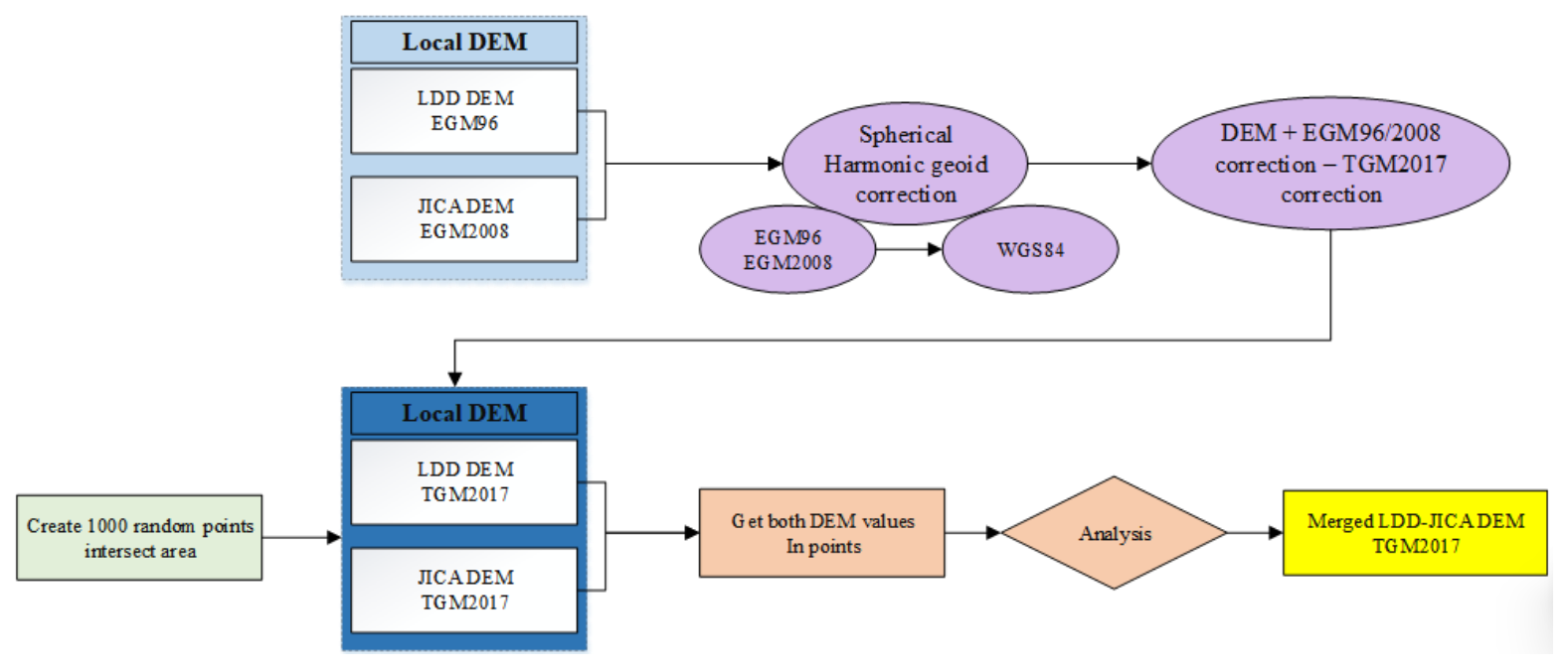
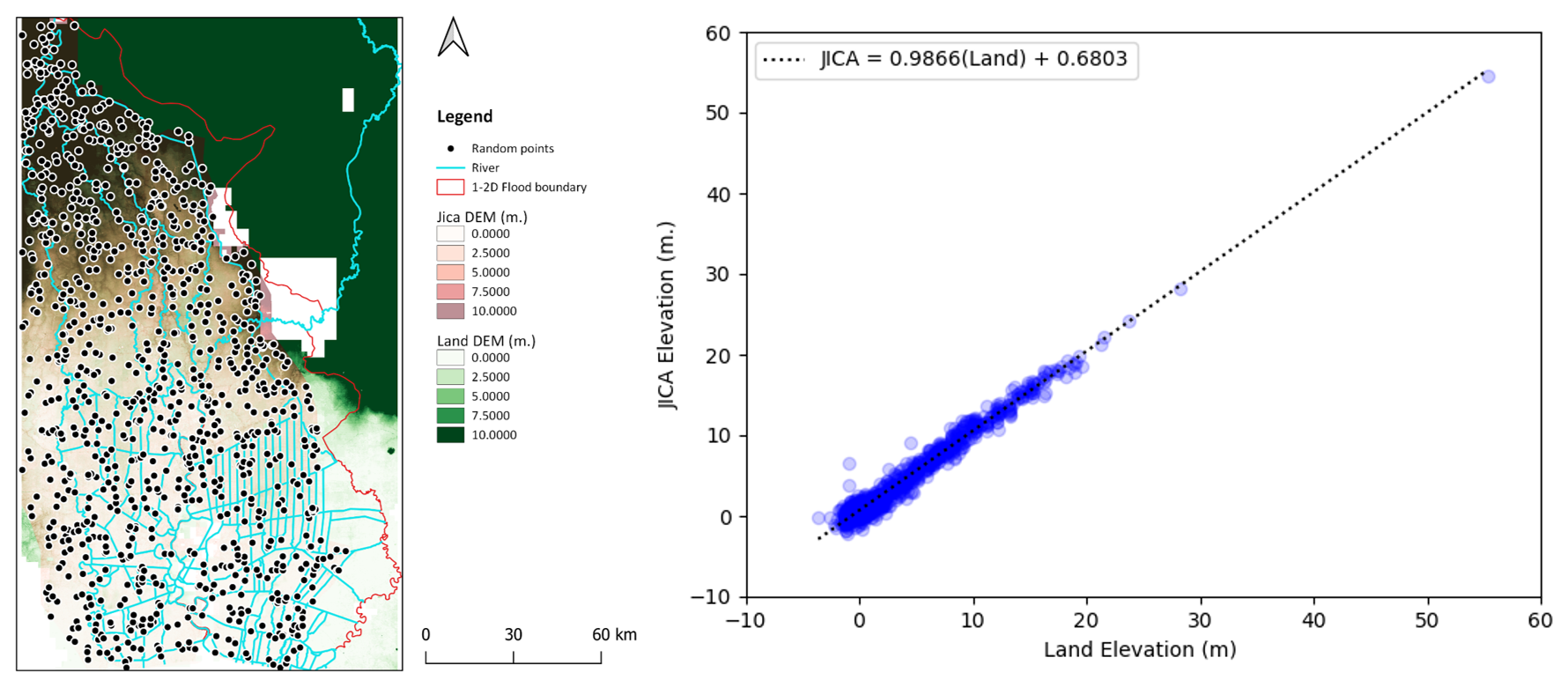
Figure A3 Merged LDD-JICA DEM processing.

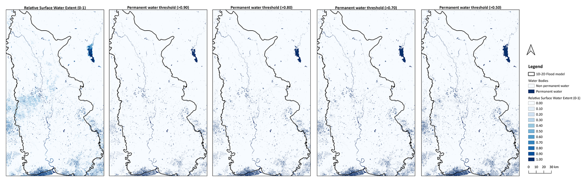
Figure A4 (a) Relative water frequency; (b) threshold, 0.9; (c) threshold, 0.8; (d) threshold, 0.7; (e) threshold, 0.5.

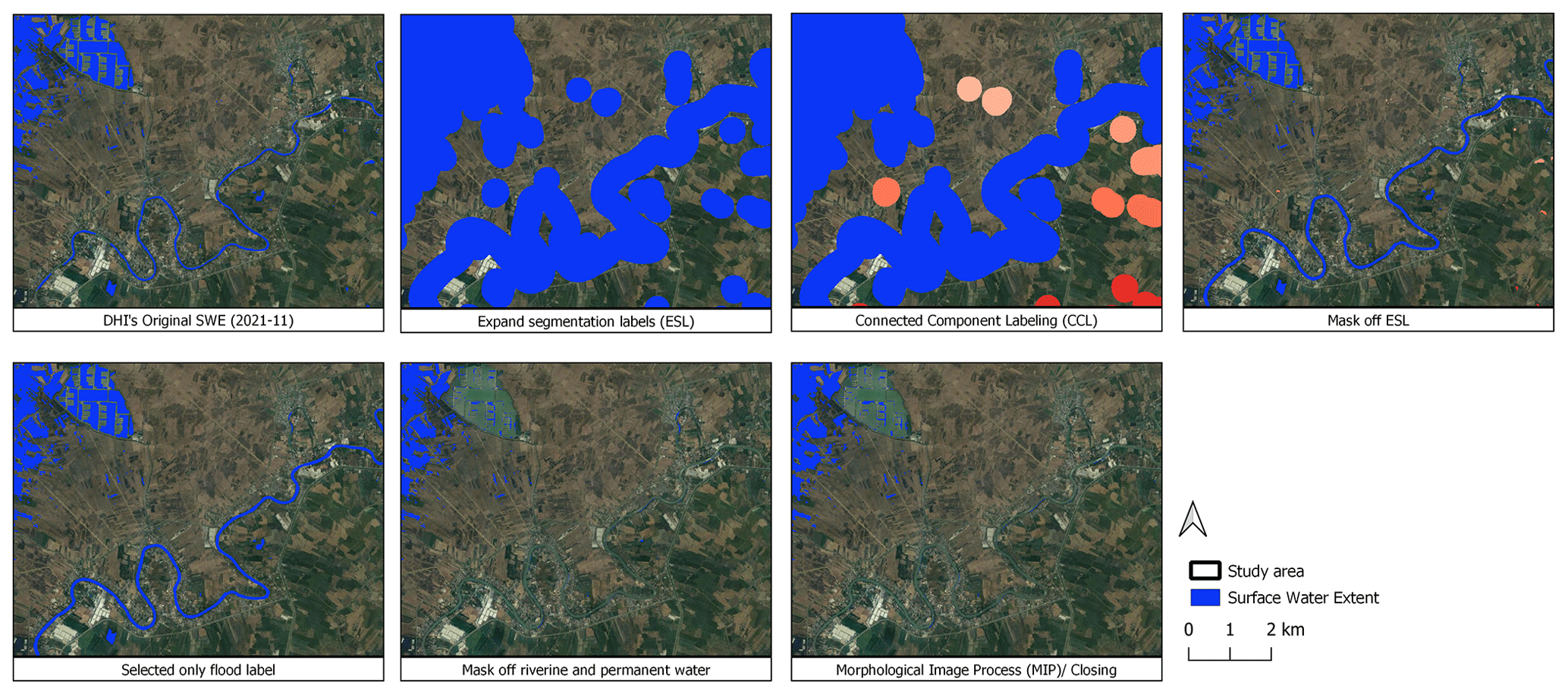
Figure A5 Riverine flood classification processing. © Google Earth 2023.

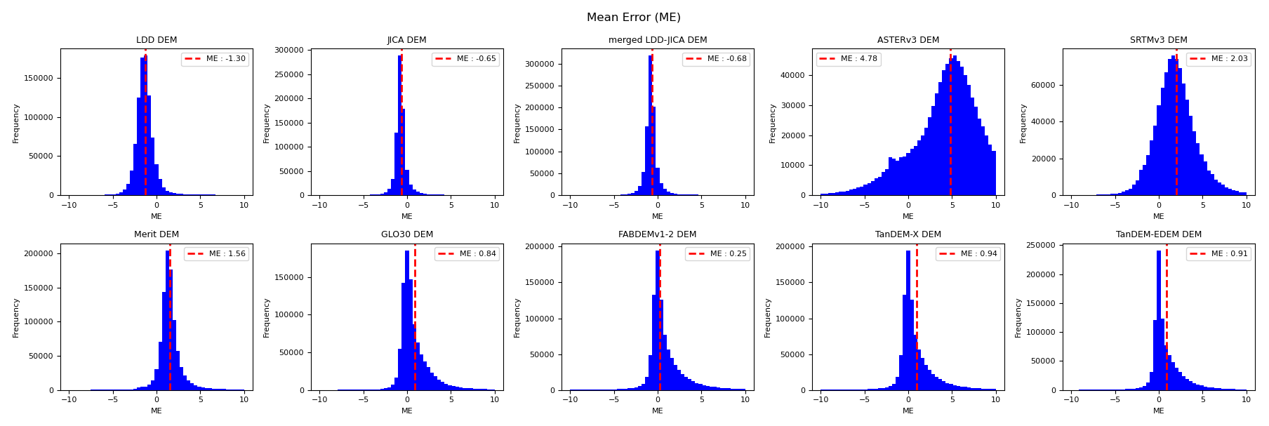
Figure A6 Histogram distribution of mean error (ME), comparing 10 DEM products against the ICESat-2 ATL08 benchmark.

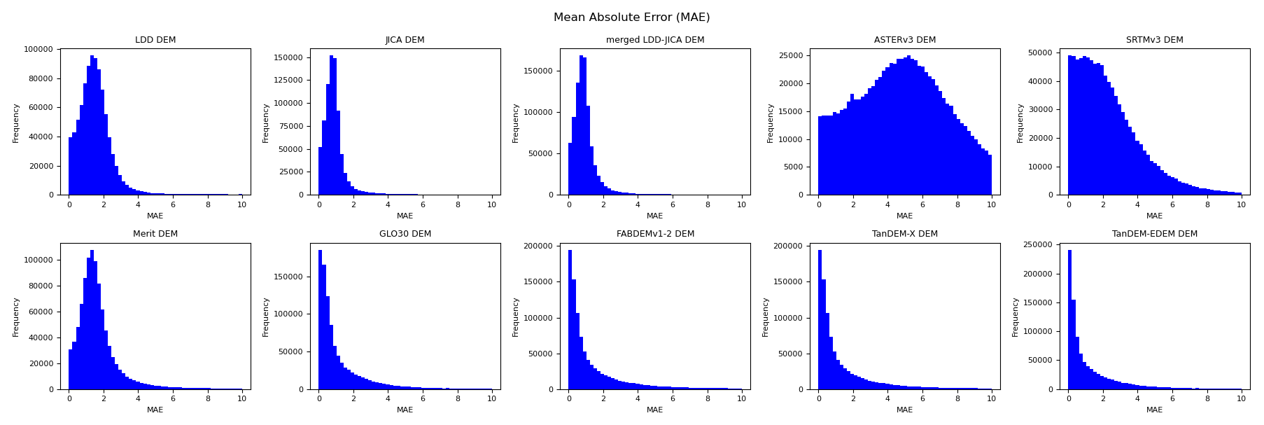
Figure A7 Histogram distribution of mean absolute error (MAE), comparing 10 DEM products against the ICESat-2 ATL08 benchmark.

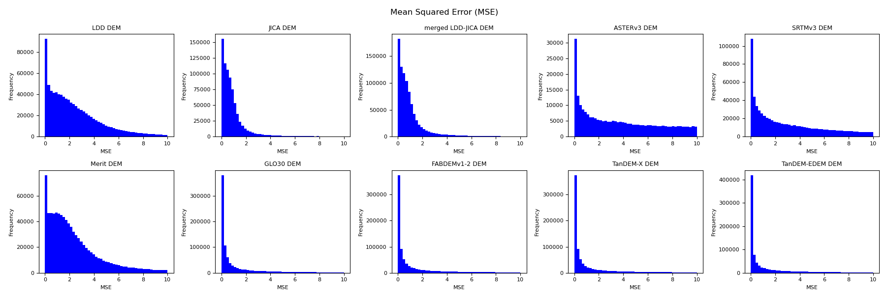
Figure A8 Histogram distribution of the mean square error (MSE), comparing 10 DEM products against the ICESat-2 ATL08 benchmark.

Figure A9 Mean error (ME) spatial grid comparison of 10 DEM products against the ICESat-2 ATL08 benchmark, with a resolution of 5 km×5 km.

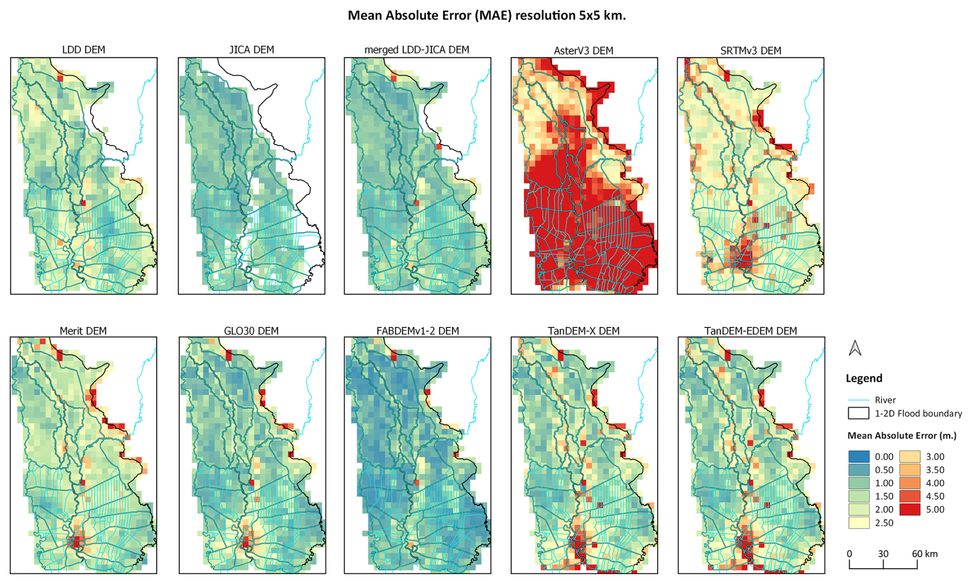
Figure A10 Mean absolute error (MAE) spatial grid comparison of 10 DEM products against the ICESat-2 ATL08 benchmark, with a resolution of 5 km×5 km.

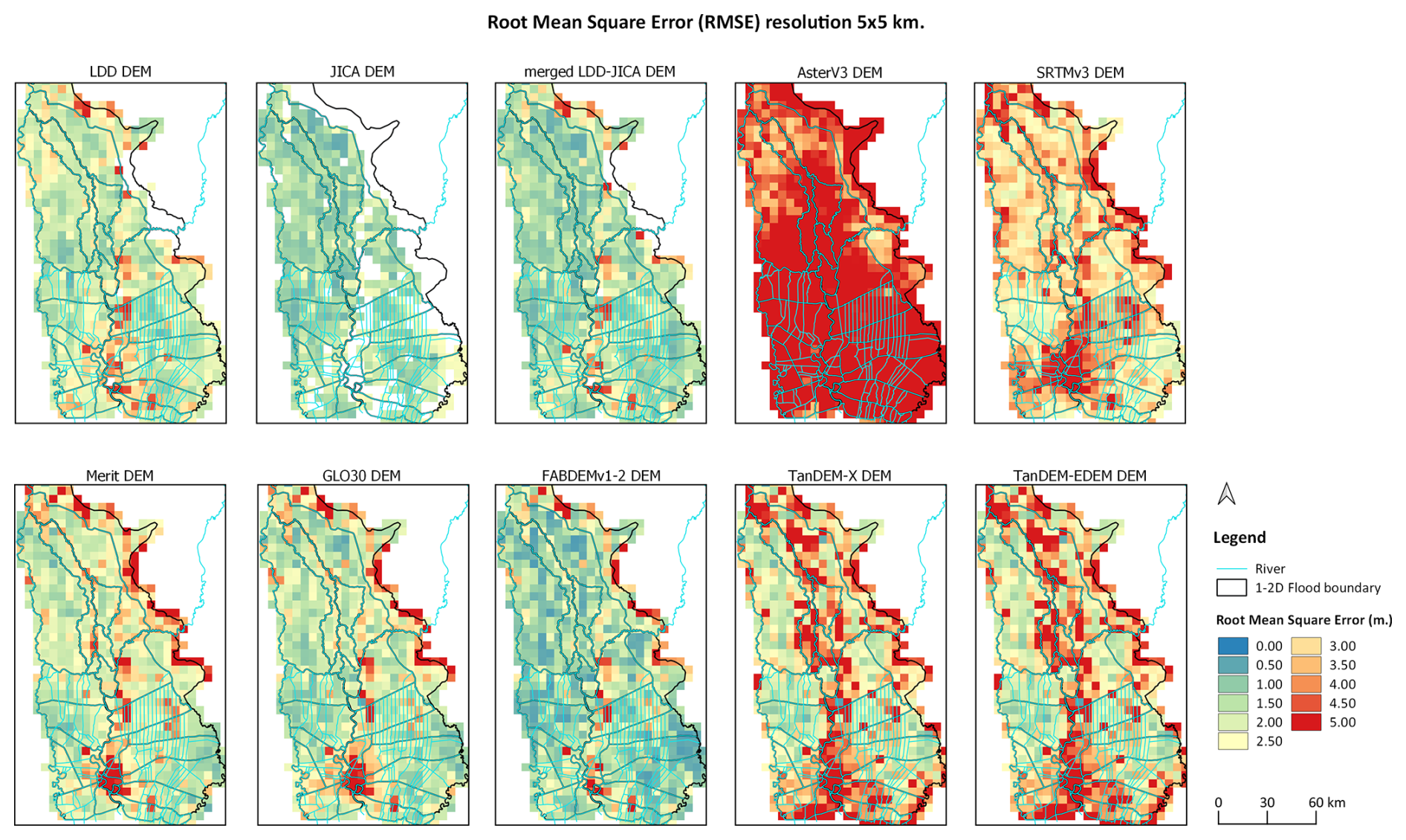
Figure A11 Root mean square error (RMSE) spatial grid comparison of 10 DEM products against the ICESat-2 ATL08 benchmark, with a resolution of 5 km×5 km.

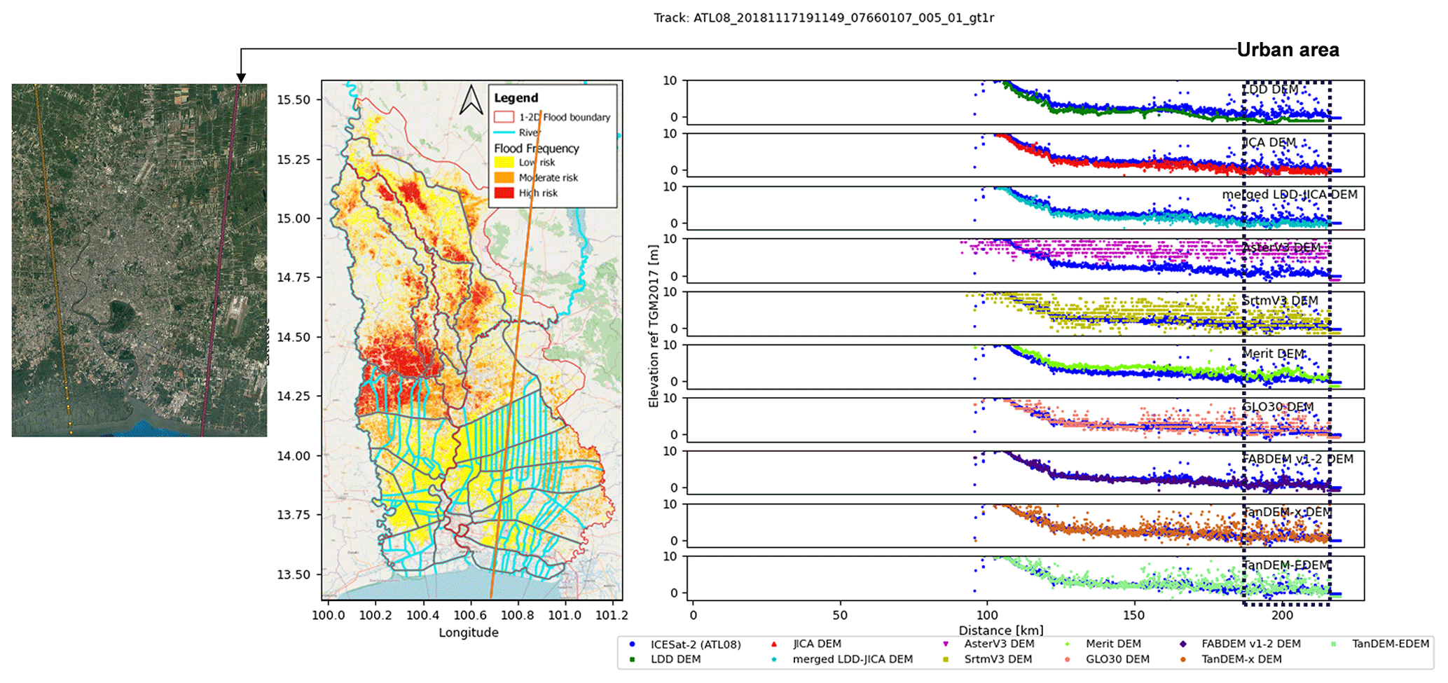
Figure A12 Track-wise comparison of 10 DEM products with ICESat-2 ATL08 benchmark. © OpenStreetMap contributors 2015. Distributed under the Open Data Commons Open Database License (ODbL) v1.0. © Google Earth 2023.