Saudi Rainfall (SaRa): hourly 0.1° gridded rainfall (1979–present) for Saudi Arabia via machine learning fusion of satellite and model data

We introduce Saudi Rainfall (SaRa), a gridded historical and near-real-time precipitation (P) product specifically designed for the Arabian Peninsula, one of the most arid, water-stressed, and data-sparse regions on Earth. The product has an hourly 0.1° resolution spanning 1979 to the present and is continuously updated with a latency of less than 2 h. The algorithm underpinning the product involves 18 machine learning model stacks trained for different combinations of satellite and (re)analysis P products along with several static predictors. As a training target, hourly and daily P observations from gauges in Saudi Arabia (n = 113) and globally (n = 14 256) are used. To evaluate the performance of SaRa, we carried out the most comprehensive evaluation of gridded P products in the region to date, using observations from independent gauges (randomly excluded from training) in Saudi Arabia as a reference (n = 119). Among the 20 evaluated P products, our new product, SaRa, consistently ranked first across all evaluation metrics, including the Kling–Gupta efficiency (KGE), correlation, bias, peak bias, wet-day bias, and critical success index. Notably, SaRa achieved a median KGE – a summary statistic combining correlation, bias, and variability – of 0.36, while widely used non-gauge-based products such as CHIRP, ERA5, GSMaP V8, and IMERG-L V07 achieved values of −0.07, 0.21, −0.13, and −0.39, respectively. SaRa also outperformed four gauge-based products such as CHIRPS V2, CPC Unified, IMERG-F V07, and MSWEP V2.8 which had median KGE values of 0.17, −0.03, 0.29, and 0.20, respectively. Our new P product – available at https://www.gloh2o.org/sara (last access: 24 September 2025) – addresses a crucial need in the Arabian Peninsula, providing a robust and reliable dataset to support hydrological modeling, water resource assessments, flood management, and climate research.

1 Introduction

The Kingdom of Saudi Arabia presents a striking hydrological paradox, experiencing periods of destructive flash floods and acute water scarcity, often simultaneously. Flash floods, the Kingdom's most frequent natural hazard, occur on average seven times a year across the country, incurring significant economic losses and social disruption (Al Saud, 2010). Particularly devastating were the flash floods in Jeddah in 2009 and 2011, claiming 113 and 10 lives, respectively, and resulting in widespread damage to property, averaging around USD 3 billion (Youssef et al., 2016). Moreover, climate change is projected to shift precipitation (P) patterns and increase atmospheric water vapor, potentially leading to more intense storms (Tabari and Willems, 2018; Almazroui et al., 2020; Fowler et al., 2021). Saudi Arabia also faces significant challenges in achieving water security for its growing population. The arid climate of the region, combined with an increasing water demand driven by rapid urbanization, industrialization, and agricultural expansion, puts immense pressure on limited water resources (Al-Ibrahim, 1991; Sultan et al., 2019). Effective management of these challenges requires accurate and timely P data, as well as assessing the impacts of climate change, developing adaptation and mitigation strategies, optimizing water resources management, and improving flash flood early warning systems. The development of such datasets is also crucial for achieving the objectives of the National Water Strategy and Vision 2030 (Ministry of Environment, Water and Agriculture, 2025), which aim to create a sustainable water sector while providing cost-effective supply and high-quality services to foster economic and social development

Huffman et al. (2019)Huffman et al. (2019)Huffman et al. (2019)Kubota et al. (2020)Kubota et al. (2020)Hersbach et al. (2020)Hersbach et al. (2020)Nguyen et al. (2020)Sadeghi et al. (2021)Kosaka et al. (2024)Joyce et al. (2004)Xie et al. (2017)Hong et al. (2004)Chen et al. (2008)Ciabatta et al. (2018a)Brocca et al. (2019)Massari et al. (2020)Funk et al. (2015)Funk et al. (2015)Beck et al. (2019b)

Table 1 Overview of quasi-global and fully global P products used in this study. Abbreviations: P = precipitation; T = temperature; S = satellite; G = gauge; Re = reanalysis; A = analysis; NRT = near-real-time; Pred = used as predictor to generate SaRa; and Eval = included in the performance assessment. The column for spatial coverage denotes “Global” for complete global coverage including ocean regions and “Land” for coverage limited to terrestrial areas. Version information unavailable for most products.

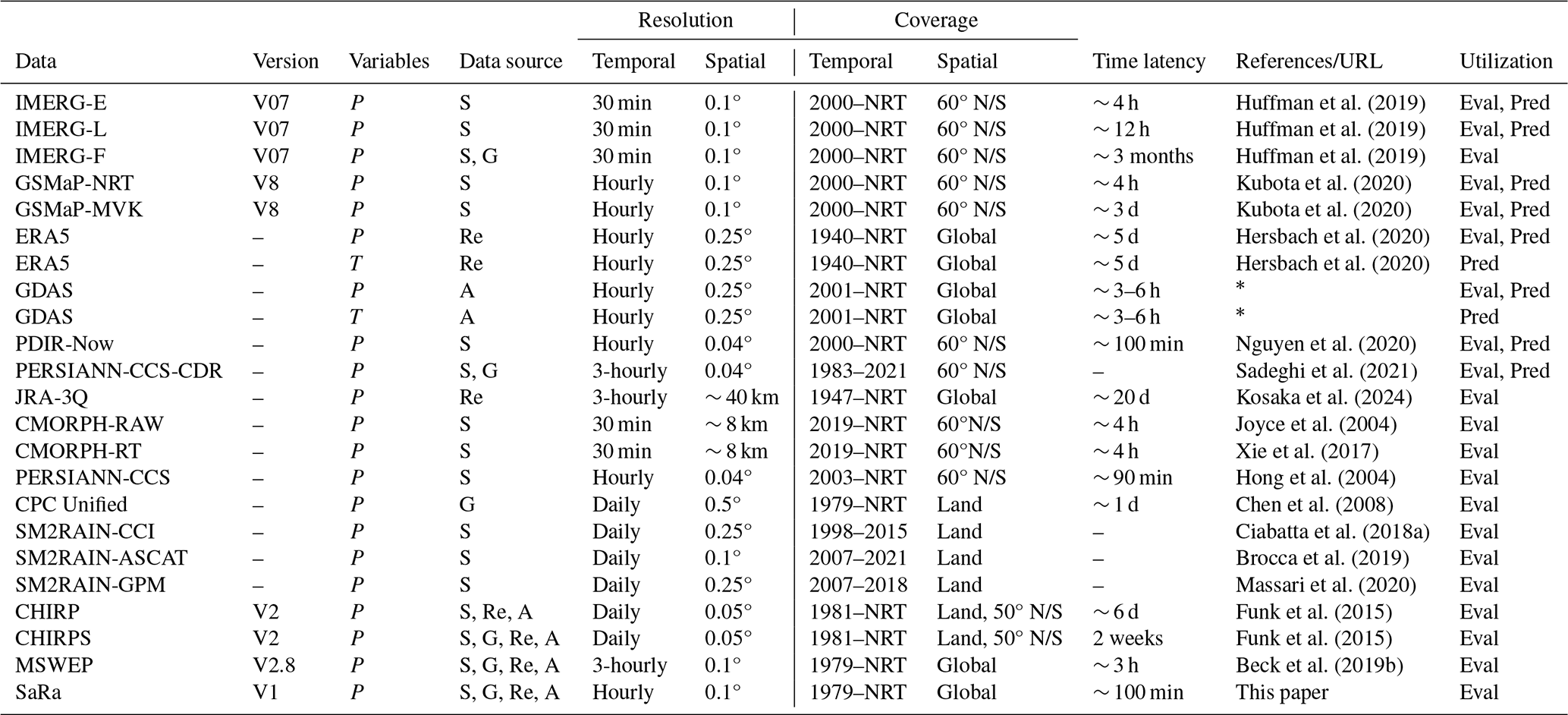
^∗ https://www.ncei.noaa.gov/products/weather-climate-models/global-data-assimilation (last access: 18 September 2025).

Over the past few decades, a wide range of gridded P products have been developed, each with unique design objectives, spatial and temporal resolutions, coverage, latency, algorithms, and data sources, ranging from satellite to analysis, reanalysis, gauges, and their combinations. Table 1 provides an overview of quasi-global and fully global products. In general, P products contain inherent errors and biases, making it important to assess their performance to determine their relative strengths, weaknesses, and suitability for different applications and utility for particular regions and geographies. While several global studies have assessed the performance of many of these products, typically using gauge P observations as reference (e.g., Beck et al., 2017; Sun et al., 2018; Nguyen et al., 2018), they have often excluded Saudi Arabia due to the scarcity of local P observations. To date, only a limited number of evaluations have specifically focused on the Arabian Peninsula (Kheimi and Gutub, 2015; Mahmoud et al., 2018; El Kenawy and McCabe, 2016; El Kenawy et al., 2019; Al-Falahi et al., 2020; Helmi and Abdelhamed, 2023; Alharbi et al., 2024; Jazem Ghanim et al., 2024). Two of these studies assessed individual satellite P products – IMERG (Mahmoud et al., 2018) and PDIR-Now (Alharbi et al., 2024) – leaving questions about the comparative performance of these products unresolved. Four other studies evaluated multiple satellite P products, including CMORPH, GSMaP, PERSIANN, SM2RAIN-ASCAT, and TMPA 3B42 (Kheimi and Gutub, 2015; El Kenawy et al., 2019; Helmi and Abdelhamed, 2023; Jazem Ghanim et al., 2024). Notably, El Kenawy et al. (2019), Helmi and Abdelhamed (2023), and Jazem Ghanim et al. (2024) reported that the products generally performed poorly and highlighted the need for caution when using them. Al-Falahi et al. (2020) evaluated some of the aforementioned satellite P products as well as the reanalysis ERA5 but only focused on the highland region of Yemen. However, many satellite products evaluated in these studies have been superseded by newer, significantly improved versions. Additionally, several promising products have not been evaluated yet, including SM2RAIN-GPM (Massari et al., 2020), MSWEP V2.8 (Beck et al., 2019b), and JRA-3Q (Kosaka et al., 2024).

Several gridded P products, such as CHIRPS V2 (Funk et al., 2015), GPCP (Huffman et al., 2023), MSWEP V2.8 (Beck et al., 2019b), and SM2RAIN-GPM (Massari et al., 2020; Table 1), leverage multiple P-related data sources to obtain improved P estimates. These products employ statistical methods to minimize errors and biases inherent in individual sources, thereby enhancing P estimation performance across various regional, seasonal, and temporal scales. Although these products generally outperform single-source P products (e.g., Beck et al., 2017; Prakash, 2019; Shen et al., 2020), machine learning (ML) approaches are increasingly recognized for their ability to efficiently fuse multiple data sources, while mitigating errors and biases. A wide variety of ML models, often trained with gauge observations, have been used for P estimation, including classical models such as multivariate linear regression (MLR), artificial neural networks (ANNs), support vector machines (SVMs), and random forests (RF) along with modern deep learning models such as convolutional neural networks (CNNs) and long short-term memory (LSTM) networks and hybrid models (see reviews by Hussein et al., 2022; Dotse et al., 2024; Papacharalampous et al., 2023; Xu et al., 2024). However, most ML studies on P estimation have limitations in that (i) they generally focus on a small region or catchment, which limits the usefulness and generalizability of the findings; (ii) they often focus on a monthly (rather than daily or sub-daily) timescale, which may not meet the needs of all applications; (iii) they develop models for either near-real-time or historical P purposes but not both; (iv) they use gauge observations as predictors, which precludes near-real-time model application, given that gauge observations are generally not available in near-real time; (v) they remain largely theoretical, often failing to offer a corresponding, accessible P dataset for users and follow-up studies. Additionally, and crucially, no study has yet investigated the potential of ML to specifically enhance P estimates in the Arabian Peninsula region.

Here, we introduce Saudi Rainfall (SaRa), a new gridded near-real-time P product with an hourly 0.1° resolution designed to overcome the aforementioned limitations. The product covers the Arabian Peninsula (Fig. 1) from 1979 to the present with a latency of less than 2 h. It was derived using ML models trained on a vast database of hourly and daily gauge P observations from around the world. The ML models are tailored to various P product combinations to ensure optimal performance for each period and location. In the following section, we describe the data and methods underlying the product. Subsequently, we (i) evaluate the performance of the ML models, constructed using different gridded P product combinations as predictors; (ii) assess SaRa's performance relative to 19 global P products; (iii) examine the spatial patterns in performance; (iv) discuss the challenges of estimating P in arid regions; and (v) present trends in average and extreme P for the Arabian Peninsula based on SaRa.

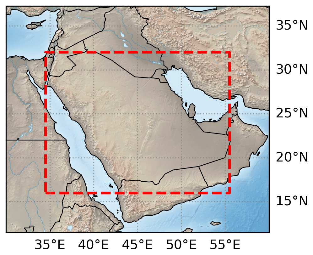
Figure 1 Study area location with SaRa dataset boundaries shown in red. Land cover data and shaded relief from Natural Earth (https://www.naturalearthdata.com/, last access: 18 September 2025).

2 Data and methods

2.1 Gridded precipitation and air temperature products

Global gridded P products (more details in Table 1) were used for two purposes: (i) as predictors to generate our new P product for the Arabian Peninsula (SaRa) and (ii) to evaluate the performance of SaRa relative to other P products. Gridded air temperature (T) data were also used as predictors to account for seasonal differences in error characteristics and relative performance among products. Throughout this paper, we refer to these global gridded predictors as “dynamic” due to their temporal variability – in contrast to predictors that are invariant in time, which are referred to as “static” (see below). We restricted our selection to P products with a daily or sub-daily temporal resolution. The P products included in our study originate from diverse sources, encompassing satellite observations, ground-based gauges, reanalyses, analyses, and combinations thereof. The ML models are trained to optimally merge the P products and mitigate errors and biases using gauge P data. The products selected as predictors for developing SaRa were primarily non-gauge-corrected P datasets to avoid biasing predictor importance, particularly in cases where the same stations used for training might have been employed to correct the respective P products. We included both microwave-based (IMERG-L V07 and GSMaP-MVK V8) and infrared-based (PERSIANN-CCS-CDR and PDIR-Now) satellite products as predictors. Among the predictors, the only gauge-corrected product is the infrared-based satellite-product PERSIANN-CCS-CDR, which has been corrected at the monthly scale using the Global Precipitation Climatology Project (GPCP) product (V2.3; monthly 2.5° resolution; Adler et al., 2018). PERSIANN-CCS-CDR was used prior to 2000, before the more accurate microwave-based satellite-products IMERG and GSMaP became available. For consistency, P and T estimates from ERA5 and GDAS were resampled from 0.25 to 0.1° using nearest neighbor to develop SaRa, while PERSIANN-CCS-CDR and PDIR-Now were resampled from 0.04 to 0.1° using averaging.

2.2 Static predictors

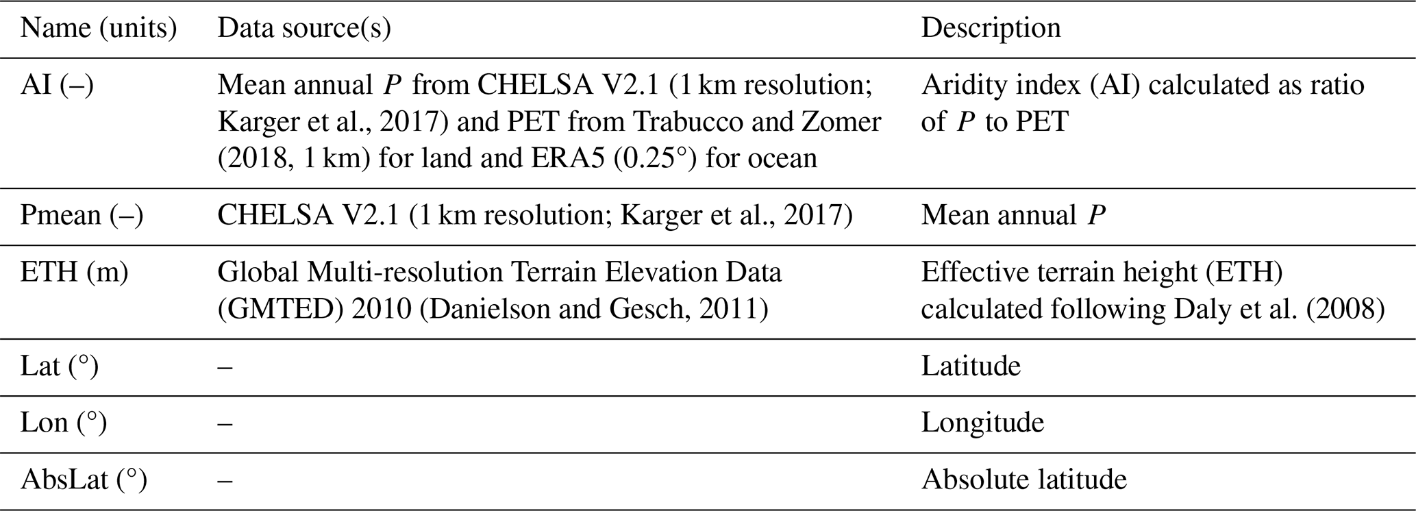
We used six static predictors to develop our new P product (Table 2). The term “static” indicates that these predictors are not time-dependent. Among these predictors, two are climate-related (Aridity Index, AI; and mean annual P, Pmean), one pertains to topography (effective terrain height, ETH), and three are linked to geographic location (latitude, longitude, and absolute latitude; Lat, Lon, and AbsLat, respectively). AI represents the ratio of mean annual P to potential evapotranspiration (PET). ETH quantifies the orographic influence on P patterns by smoothing the topography (Daly et al., 2008). We excluded slope from our predictors as it was strongly correlated with ETH. Air temperature was omitted because it is already included as a dynamic predictor. Each static predictor was resampled by averaging to match the resolution of SaRa (0.1°).

Karger et al., 2017Trabucco and Zomer (2018, 1 km)Karger et al., 2017(Danielson and Gesch, 2011)Daly et al. (2008)

Table 2 Overview of the static predictors used in the ML models to generate our new P product, SaRa.

2.3 Precipitation observations

We used P observations for two purposes: (i) as a target to train the ML models underpinning our new P dataset, SaRa, and (ii) as a reference to evaluate the performance of SaRa relative to other P products (Fig. 2). Although the SaRa product was specifically developed for the Arabian Peninsula, to account for the lack of hourly P data in the Arabian Peninsula and to enhance the generalizability of the ML models, we trained the models using P observations from across the globe. This approach assumes that valuable insights from other regions can help optimize the merging of P products and reduce errors and biases in the Arabian Peninsula. Essentially, knowledge is transferred from data-rich (gauged) to data-poor (ungauged) regions, akin to regionalization techniques typically used in hydrology to tackle Predictions in Ungauged Basin (PUB) problems, which is considered a “grand challenge” in hydrology (Sivapalan et al., 2003; Hrachowitz et al., 2013).

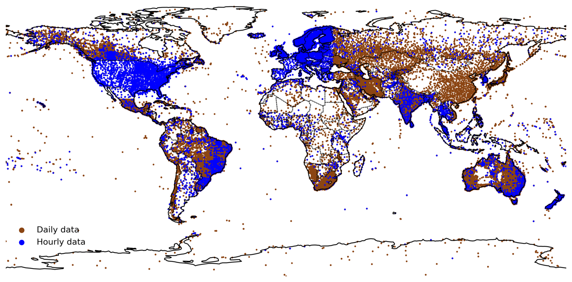
Figure 2 Global map of the 104 346 gauges remaining after duplication checks and quality control. Stations with hourly data are shown in blue, while stations with daily data are shown in brown.

For Europe and the conterminous US, our observational P data sources used for training and as reference were gridded P datasets based on gauge and radar data. Specifically, we used the EUropean RADar CLIMatology (EURADCLIM) dataset (hourly 2 km resolution; 2010–2022; Overeem et al., 2023) for Europe and the Stage-IV dataset (hourly 4 km resolution; 2002–present; Lin and Mitchell, 2005) for the conterminous US. To ensure the highest data quality, we extracted time series only at gauge locations from these datasets after resampling the data to the resolution of SaRa (0.1°) using averaging. We opted for these gauge–radar datasets over direct gauge observations in these regions because they (i) provide grid-cell averages with probability distributions (e.g., peak magnitudes and P frequencies) matching those needed for SaRa (reducing the point- to grid-scale mismatch; Yates et al., 2006; Ensor and Robeson, 2008); (ii) are expressed in UTC, avoiding temporal shifts (Beck et al., 2019b; Yang et al., 2020); and (iii) have undergone extensive quality control (Lin and Mitchell, 2005; Overeem et al., 2023).

Outside Europe and the conterminous US, we used daily and hourly gauge P observations from various national, regional, and global data sources. The daily P data sources include (i) the Global Historical Climatology Network-Daily (GHCN-D) dataset (ftp://ftp.ncdc.noaa.gov/pub/data/ghcn/daily/ (last access: 18 September 2025); Menne et al., 2012; 40 867 gauges); (ii) the Global Summary Of the Day (GSOD) dataset (https://data.noaa.gov, last access: 18 September 2025; 9904 gauges); (iii) the Latin American Climate Assessment & Dataset (LACA&D) dataset (225 gauges); (iv) the Chile Climate Data Library (712 gauges); and (v) national datasets for Brazil (10 963 gauges; https://www.snirh.gov.br/hidroweb/apresentacao, last access: 18 September 2025), Mexico (3908 gauges), Peru (255 gauges), Iran (3100 gauges), and Saudi Arabia (459 gauges). The hourly P observations encompassed 2312 gauges from the Global Sub-Daily Rainfall (GSDR) dataset (Lewis et al., 2019) produced as part of the INTElligent use of climate models for adaptatioN to non-Stationary hydrological Extremes (INTENSE) project (Blenkinsop et al., 2018), 12 585 from the Integrated Surface Database (ISD) stations (Smith et al., 2011), and national gauges from Brazil (289 gauges).

The training and evaluation of the ML model stacks used to generate SaRa was carried out for the period 2010–2024. We used this period instead of the full 1979 to the present period to reduce the significant memory requirements associated with hourly data. Additionally, EURADCLIM data start in 2010, most Saudi Arabian gauge records begin in 2014, and GDAS data start in 2021.

2.4 Duplicates check and quality control

As we used P observations from a diverse range of data sources, there was an increased risk of some gauges being included in multiple sources. To avoid over-representation of these gauges in the training set and ensure the same data were not used for both training and evaluation, we removed these duplicates. To this end, we iterated over all gauges, and if another gauge was located within a 2 km radius, we gave preference to the source we deemed most reliable. We used the following order of most to least reliable source: EURADCLIM, Stage-IV, GHCN-D, GSDR, ISD, Bolivia, Brazil, Chile, Mexico, Iran, LACA&D, GSOD, and MEWA.

P observations are often subject to systematic, gross, and random errors (Kochendorfer et al., 2017; Tang et al., 2018), which can adversely affect the training and evaluation results. We identified and filtered out potentially erroneous gauges using the following five criteria: (i) non-zero minimum daily P, (ii) daily maximum less than 10 mm d⁻¹ or exceeding 1825 mm d⁻¹ (the highest daily rainfall ever recorded; https://www.weather.gov/owp/hdsc_world_record, last access: 18 September 2025), (iii) mean annual P less than 5 mm yr⁻¹ or exceeding 10 000 mm yr⁻¹, (iv) fewer than five P events (using a 1 mm d⁻¹ threshold), and/or (v) fewer than 365 daily values (not necessarily consecutive) during 2010–2024 (the training and evaluation period). In total, 75 833 gauges were discarded out of 104 346 after these steps.

2.5 SaRa precipitation estimation algorithm

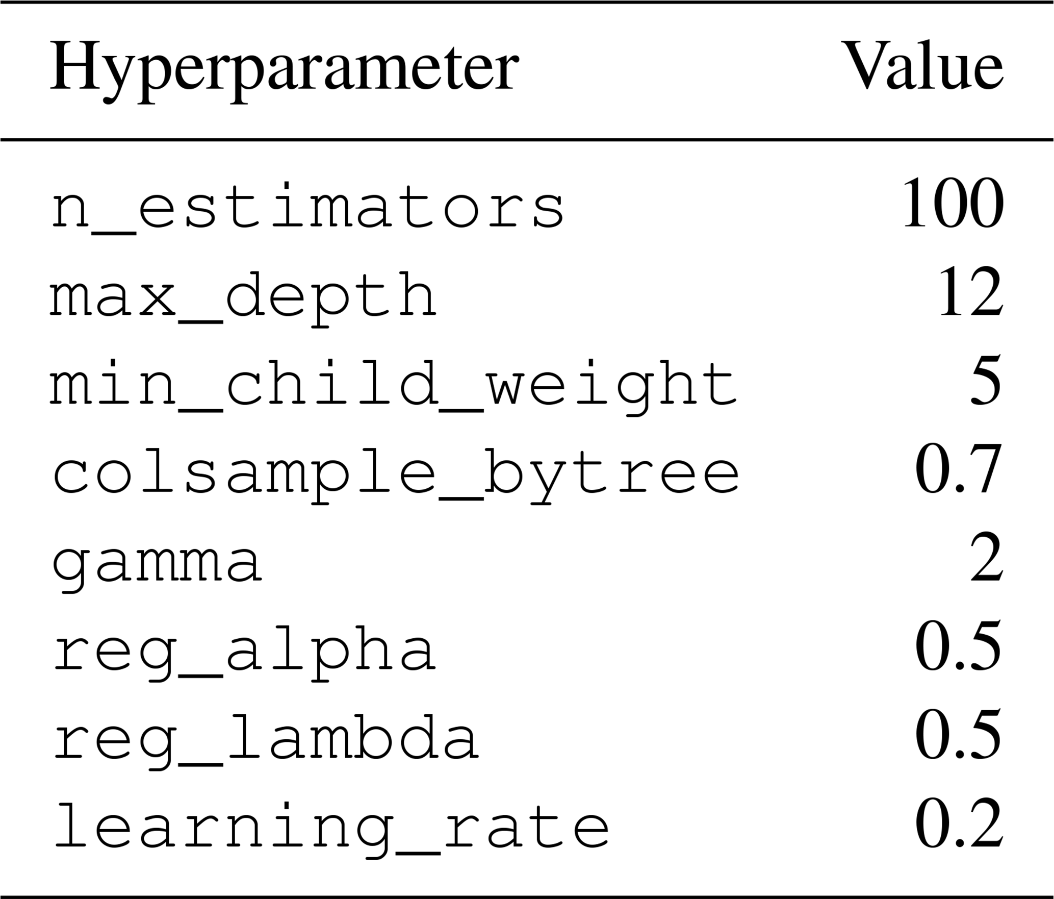
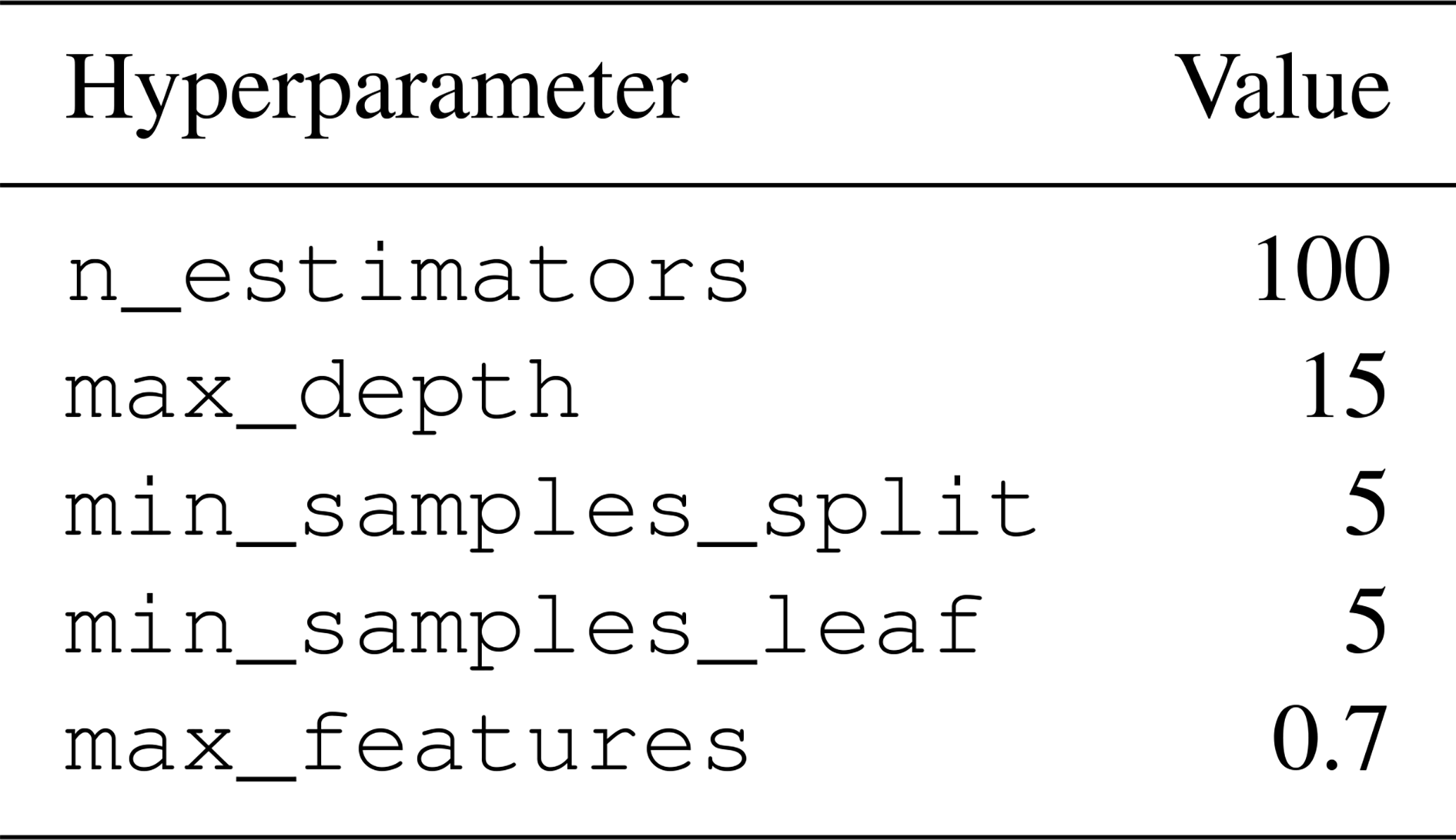
The SaRa product was derived using different ML model stacks trained from different combinations of dynamic P and T predictors (Sect. 1) along with several static predictors (Table 2). Each model stack is comprised of four separate ML submodels (Fig. 3). The first submodel is a daily XGBoost model (Chen and Guestrin, 2016) trained using daily P observations, leveraging the broad availability of P observations globally and in the Arabian Peninsula (Fig. 2). The second submodel, also based on XGBoost, disaggregates the daily estimates to 3-hourly and is trained using 3-hourly P observations, which are scarce in the Arabian Peninsula. As such, all of the 3-hourly disaggregation skill originates from other regions. As the resulting P estimates tend to underestimate the variance (i.e., generate excessive drizzle and underestimate peaks) due to the regression towards the mean phenomenon (see, e.g., He et al., 2016; Ting, 2025), a third submodel based on random forest (RF; Breiman, 2001) corrects the 3-hourly P probability distribution. The RF submodel is trained by separately sorting, for each gauge, (a) the 3-hourly estimates from the second submodel corrected using the daily estimates from the first submodel and (b) the 3-hourly P observations. To ensure the number of wet days and low P intensities are also adequately corrected, the P estimates are square-root-transformed before being fed to the third submodel and the output of the third submodel is squared. The fourth submodel disaggregates the 3-hourly estimates to hourly and also represents an XGBoost model, trained using hourly P observations.

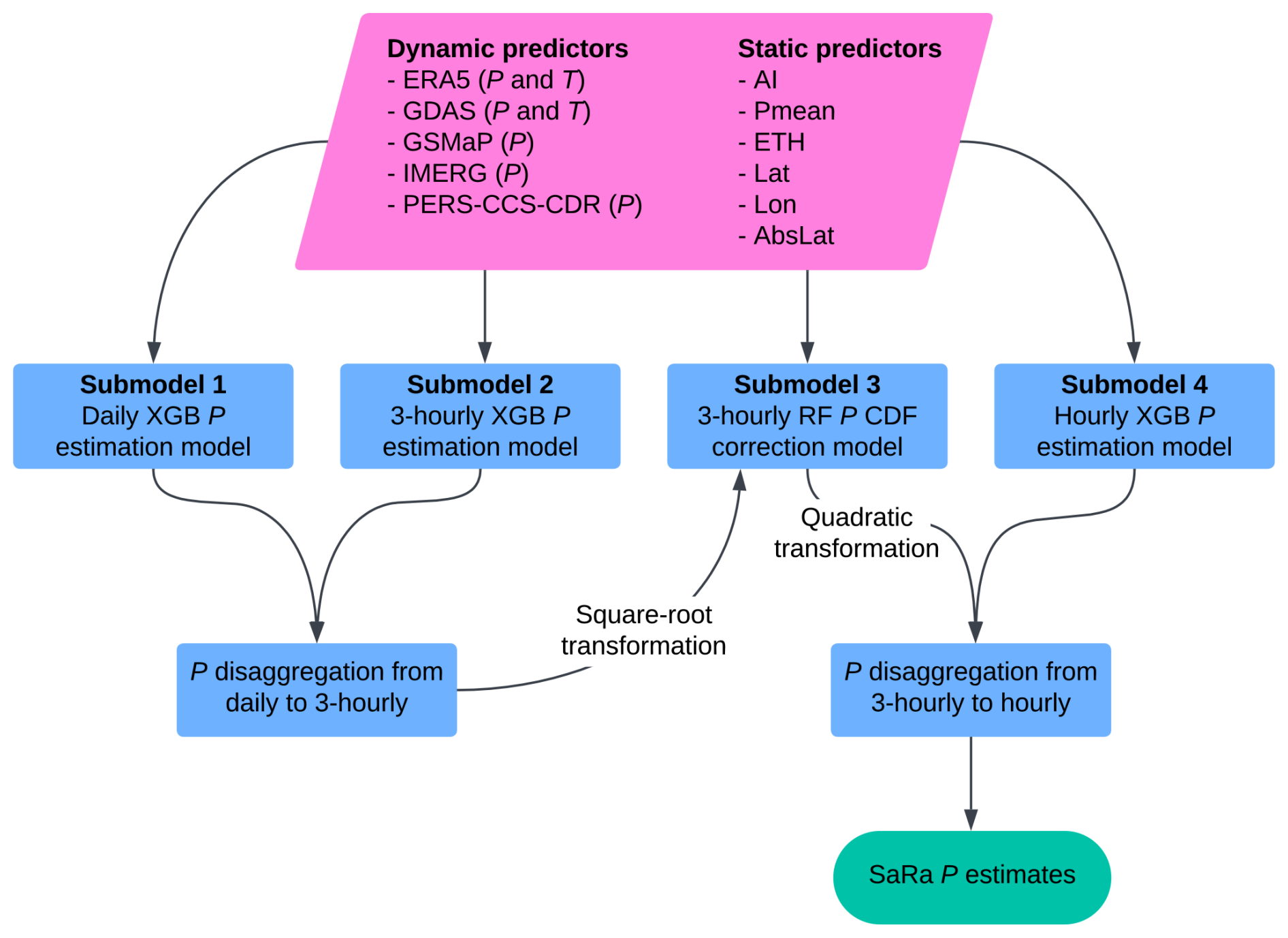
Figure 3 Flowchart of ML model stacks used to produce the new SaRa P product presented in this study.

Table 3 The dynamic predictors incorporated in the different ML model stacks.

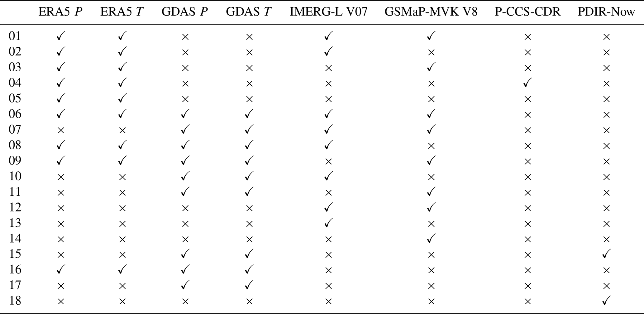
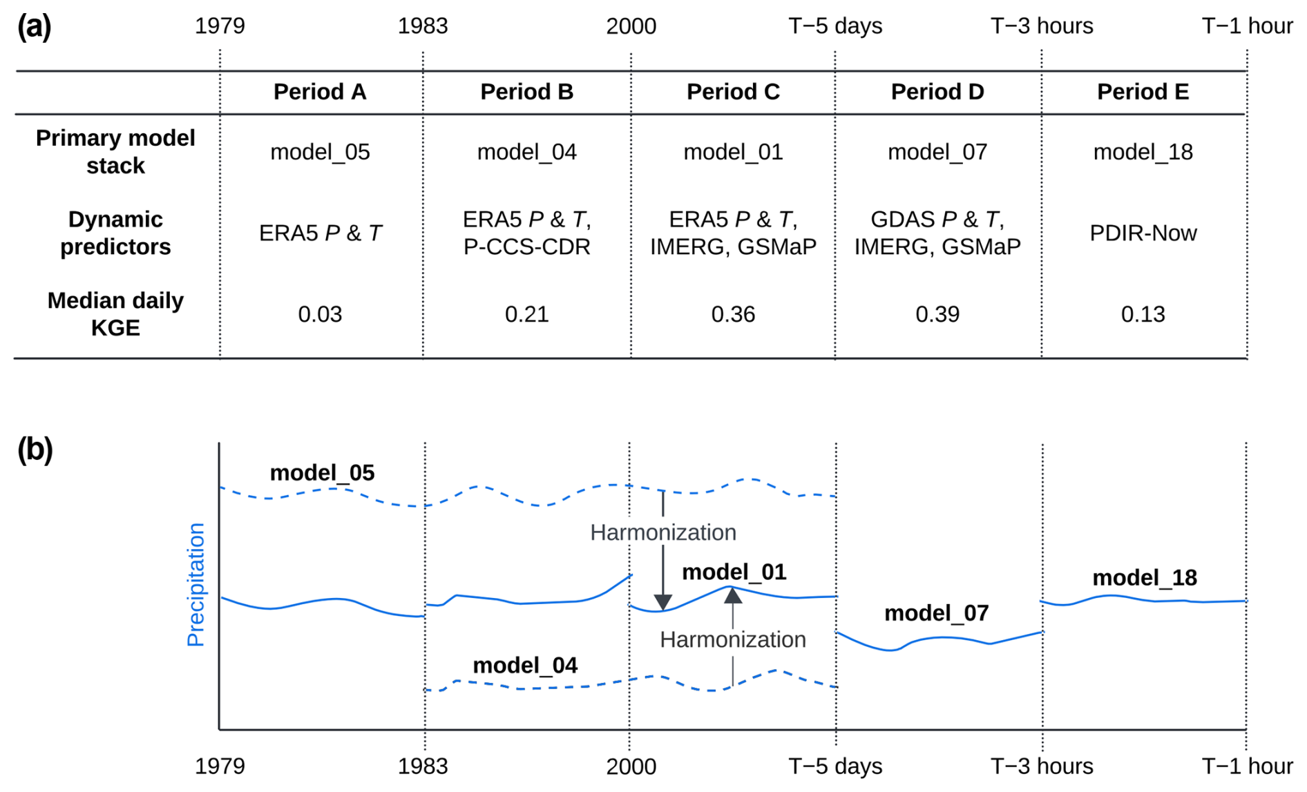
Figure 4 (a) Different ML model stacks were used for different periods and locations to account for differences in the spatio-temporal availability of the dynamic predictors. The primary ML model stack, the corresponding dynamic predictors, and the mean daily independent validation KGE (from Table 4) are also provided. Note that other ML model stacks may be used for a particular period when any dynamic predictor is not available. (b) Conceptual illustration of how P estimates from different ML model stacks are combined and how outputs from ML model stacks with long records are harmonized with the reference (model_01).

The dynamic predictors span different time periods and different regions (see Table 1), so we cannot use a single ML model stack for every time step and grid cell. We therefore trained a total of 18 different ML model stacks with various combinations of dynamic predictors (Table 3). These model stacks are used based on the available dynamic predictors for a specific time and location (Fig. 4), with preference given to the model stack with the lowest number (e.g., model_01 is preferred over model_02). The final SaRa P estimates were generated by iterating over all 0.1° grid cells, loading all dynamic and static predictors, and then applying the preferred ML model stack. To avoid temporal discontinuities, such as around 1983 when PERSIANN-CCS-CDR was introduced or in 2000 when IMERG and GSMaP were introduced, the outputs from model_04 and model_05 were harmonized with the outputs of model_01, which we consider the reference due to its long record (from 2000 to 5 d prior to the present) and high accuracy (owing to the availability of ERA5, IMERG, and GSMaP). The harmonization process involved (i) detrending the time series by dividing by the moving annual average, (ii) cumulative distribution function (CDF) matching, and (iii) multiplying the result by the moving annual average (Fig. 4). The detrending serves to avoid amplification of trends in extreme P (see, e.g., Cannon et al., 2015).

We implemented the RF models using the scikit-learn package and XGBoost models using the XGBoost package in Python. The hyperparameters we used are summarized in Appendix A.

2.6 Training and evaluation

Both the training and evaluation were carried out for the period 2010–2024, aligning with the temporal coverage of EURADCLIM and the Saudi gauge data. From the 28 513 gauges that passed the duplicates check and quality control (Sect. 2.4), we randomly allocated 50 % for training (14 256 gauges) and the remaining 50 % for evaluation. We trained submodel one using all available daily gauge data, while submodels two, three, and four were trained using gauges with hourly data (aggregated to 3-hourly for submodels two and three). The specific number of gauges used for training each model stack depends on the temporal span and spatial coverage of the dynamic predictors. Since GDAS covers a relatively short period (2021 to the present), any ML models incorporating GDAS were trained using a significantly smaller number of observations.

The time stamps of the hourly P observations may reflect the local time zone instead of coordinated universal time (UTC), while the daily P observations may represent accumulations ending at various times, not necessarily at midnight UTC (Yang et al., 2020). Such discrepancies can lead to temporal mismatches between the dynamic predictors on one side and the gauge P observations on the other, thereby hindering satisfactory model training. To address this issue, we determined time shifts in the hourly and daily gauge P data using the hourly satellite-based IMERG-L V07 and GSMaP-MVK V8 products, similar to Beck et al. (2019b). To determine hourly gauge data shifts, we shifted the gauge record by 1 h increments from −36 to +36 and calculated the average Spearman correlations between shifted gauge data and IMERG-L V07/GSMaP-MVK V8 data. To determine daily gauge data shifts, we shifted the IMERG-L V07 and GSMaP-MVK v8 data separately by 1 h increments from −36 to +36, computed daily P accumulations from the shifted IMERG-L V07 and GSMaP-MVK V8 data, and calculated the average Spearman correlations between daily gauge record and shifted IMERG-L V07/GSMaP-MVK V8 data. The shifts that yielded the highest correlations were then used to recalculate daily values of the dynamic predictors for training ML submodel one, as well as shifting the hourly gauge records for training submodels two and four.

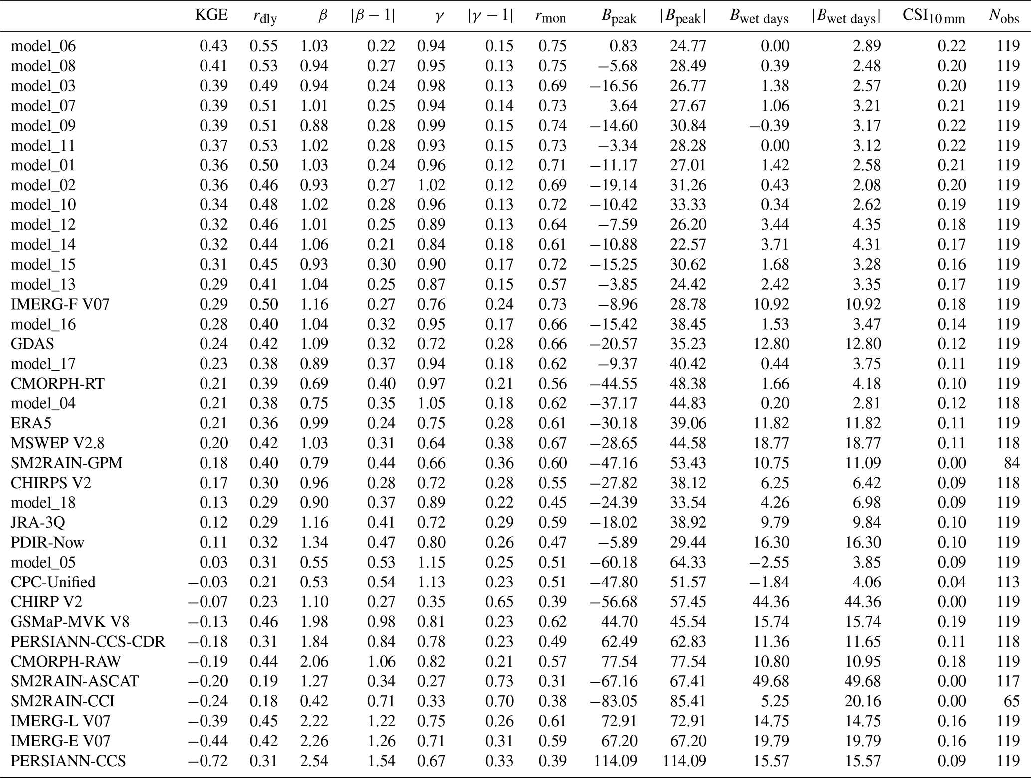
Table 4 The performance of the ML model stacks underlying our new P product SaRa (models_01–18) and other state-of-the-art P products sorted in descending order of median KGE. The values represent medians calculated over all randomly selected independent evaluation gauges in Saudi Arabia. Note that since the different P products span different temporal periods, the specific evaluation data used for the evaluation differ between P products. The unit for B_peak is %, and the unit for B_wet days is the number of days. N_obs indicates the number of stations used to assess each product.

The 119 randomly selected evaluation gauges are completely independent and were not used to train the ML models, enabling a thorough performance assessment of SaRa compared to other P products (Table 4). We used several performance metrics for a comprehensive evaluation: (i) the Kling–Gupta efficiency (KGE; Gupta et al., 2009; Kling et al., 2012), which is an aggregate metric combining Pearson correlation (r_dly), overall bias (β), and variance bias (γ); (ii) monthly Pearson correlation (r_mon); (iii) peak bias at the 99.5th percentile (B_peak; %); (iv) wet-day bias (B_wet days, days; calculated using a 0.5 mm d⁻¹ threshold); and (v) Critical Success Index (CSI), measuring the ratio of hits to the sum of hits, false alarms, and misses for P events exceeding 10 mm d⁻¹. These metrics, selected to encompass all important aspects of P time series, were computed for each evaluation gauge based on daily data, except for r_mon. We did not conduct an hourly evaluation due to the lack of hourly observations in the Arabian Peninsula. For a detailed explanation of the performance metrics, including the equations, see Appendix B.

3 Results and discussion

3.1 Performance of ML models

To generate the SaRa product, we trained 18 different ML model stacks with different P product combinations (Table 3). The performance of these models in terms of median KGE, calculated using daily P data from independent evaluation gauges, ranges from 0.03 for model_05, which relies solely on one dynamic P predictor (ERA5), to 0.43 for model_06, which incorporates four dynamic P predictors (ERA5, GDAS, IMERG-L V07, and GSMaP-MVK V8; Table 4). These results align with our expectation that models incorporating a larger number of dynamic predictors are able to extract complementary strengths from them, resulting in better performance. model_01, based on three dynamic P predictors (ERA5, IMERG-L V07, and GSMaP-MVK V8), is arguably the most important ML model stack as it covers the largest portion of the record, from 2000 to 5 d prior to the present, and also performs well, achieving a median KGE of 0.36, a median peak bias (B_peak) of −11.17 %, a wet-day bias (B_wet days) of +1.42 d, and a median weather event detection score (CSI_10 mm) of 0.21.

The B_peak value of −11.17 % obtained by model_01 suggests a slight underestimation of high rainfall amounts (Table 4). Although ML models are known to underestimate extremes due to the regression toward the mean phenomenon (see, e.g., He et al., 2016), the most likely reason is that the gauge P data used for evaluation represent point measurements, which typically exhibit higher peaks than grid-cell averages (Ensor and Robeson, 2008). Thus, this apparent underestimation may primarily reflect a scale discrepancy. Similarly, the B_wet days value of +1.42 d (Table 4), indicating a minor overestimation of rainfall frequency, might also be attributable to this scale difference. Rainfall frequencies are generally higher for grid-cell averages than for point measurements (Osborn and Hulme, 1997). Note that a significant portion of the training data comprises gridded gauge–radar P data (see Sect. 2.3), which have a 0.1° grid-cell-scale consistent with SaRa.

Among all the trained ML model stacks, model_05 performed the worst, with a median KGE of 0.05. model_05 uses only one dynamic predictor (ERA5) and is designed primarily for the period before 1983, when only ERA5 data are available (Fig. 4). It also performs worse than ERA5 alone (median KGE of 0.21), which is mainly attributable to poor bias (β) and peak bias (B_peak) values. Fortunately, these issues are largely resolved during the harmonization step, where the outputs of model_04 and model_05 are harmonized with those of model_01, which is considered the reference (Fig. 4).

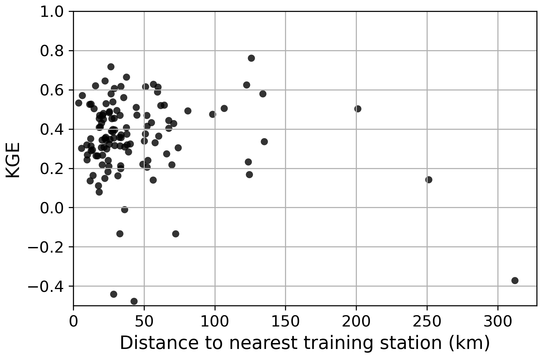
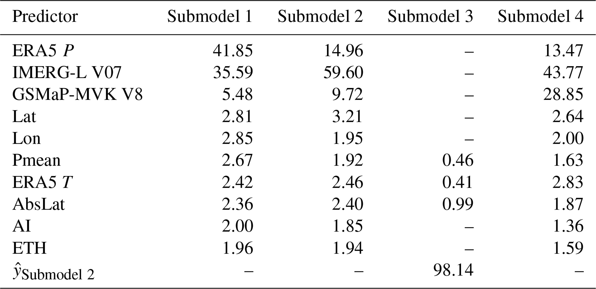
A key potential limitation of ML-based P estimation is poor generalizability; models often fail in regions lacking training data (Xu et al., 2024). To assess whether this applies to our models, we analyzed KGE values of the evaluation stations as a function of distance to the nearest training station (Fig. 5). The results show no clear decline in KGE with increasing distance, indicating satisfactory spatial generalizability. Another potential limitation is the “black-box” nature of ML models, which limits interpretability. To improve transparency, we computed predictor importance for all four submodels of model_01 (Table 6). IMERG-L V07 consistently ranked higher than GSMaP-MVK V8 in importance, indicating a preference for IMERG, in agreement with its superior validation performance (Table 4). ERA5 was the most important predictor for the daily submodel (Submodel 1), whereas IMERG dominated in the 3-hourly and hourly submodels (Submodels 2 and 4, respectively). This likely reflects the ability of observational satellite-based datasets like IMERG to capture event timing more accurately. This also demonstrates the ability of the models to exploit the complementary strengths of the different P predictors. Static predictors were overall much less important than dynamic ones. Among the static predictors, Lon, Lat, and AbsLat had the highest importance, accounting for regional variability in P predictor performance and error characteristics.

Figure 5 KGE versus distance to nearest training station for the evaluation stations (n=119). The same KGE values are also presented in Fig. 6a.

3.2 Performance comparison with other gridded P products

The primary model underlying our newly developed SaRa product, model_01, exhibited superior performance across nearly all 12 performance metrics relative to all 19 other P products (Table 4). Notably, model_01 attained a median KGE of 0.36, significantly outperforming widely used P products such as ERA5, JRA-3Q, CMORPH-RT, CHIRPS V2, IMERG-L V07, GSMaP MVK V8, and MSWEP V2.8, which obtained median KGE values of 0.21, 0.12, 0.21, 0.17, −0.39, −0.13, and 0.2, respectively. Additionally, model_01 performed well in terms of high P intensities, exhibiting a low peak bias (B_peak) of −11.17 %, while the aforementioned other P products showed higher biases of −30.18 %, −18.02 %, −44.55 %, −27.82 %, +72.91 %, +44.7 %, and −28.65 %, respectively. In terms of detecting P events (CSI_10 mm), model_01 scored a median value of 0.22, surpassing the other products with values ranging from 0.09 to 0.19.

Although SaRa was derived using an algorithm trained on gauge P observations (from stations excluded in the evaluation), it was not directly corrected using gauge observations. Despite this, SaRa outperformed products entirely based on gauge observations (CPC Unified) or corrected using gauge observations (CHIRPS V2, IMERG-F V07, and MSWEP V2.8). This mainly reflects the limited availability of gauge observations from Saudi Arabia in global databases like GHCN-D (Menne et al., 2012; Kidd et al., 2017). Additionally, the lower performance of CHIRPS V2 and IMERG-F V07 may stem from their 5 d and monthly gauge corrections, respectively, which are less effective at improving performance on a daily timescale.

Among the purely (re)analysis-based products (ERA5, GDAS, and JRA-3Q), GDAS performed best with a median KGE of 0.24, outperforming ERA5 (median KGE of 0.21) and JRA-3Q (median KGE of 0.12; Table 4). Among the microwave satellite-based products (CMORPH-RT and -RAW, GSMaP-MVK V8, IMERG-L and IMERG-E V07, and SM2RAIN-GPM), CMORPH-RT emerged as best (median KGE of 0.21), followed by SM2RAIN-GPM (median KGE of 0.18) and GSMaP-MVK V8 (median KGE of −0.13). Among the purely infrared satellite-based products (PERSIANN-CCS and PDIR-Now), PDIR-Now performed best (median KGE of 0.11). PDIR-Now also outperformed some microwave-based products (GSMaP-MVK V8, IMERG-L, and IMERG-E V07). Among the SM2RAIN products (SM2RAIN-GPM, SM2RAIN-ASCAT, and SM2RAIN-CCI), SM2RAIN-GPM obtained the best overall performance (median KGE of 0.18). SM2RAIN-ASCAT and SM2RAIN-CCI performed poorly, exhibiting CSI_10 mm values of 0.00, underscoring the limited capability of algorithms that infer P based on soil moisture signals to detect P events > 10 mm d⁻¹ over the Arabian Peninsula. This is likely due to the extremely arid conditions in the Arabian Peninsula, where the soil dries out rapidly following P events, reducing the effectiveness of soil moisture-based detection methods. These results are in agreement with Jazem Ghanim et al. (2024), who also found SM2RAIN-ASCAT to perform poorly in the Arabian Peninsula.

Previous studies that evaluated P datasets for the Arabian Peninsula include Kheimi and Gutub (2015), Mahmoud et al. (2018), El Kenawy and McCabe (2016), El Kenawy et al. (2019), Al-Falahi et al. (2020), Helmi and Abdelhamed (2023), Alharbi et al. (2024), and Jazem Ghanim et al. (2024). Comparing our results to these studies is challenging because they assessed fewer P products and used outdated versions. However, Alharbi et al. (2024) reported a mean r_dly of 0.33 for PDIR-Now, which is comparable to our median value of 0.32 (Table 4). Similarly, Helmi and Abdelhamed (2023) reported KGE, r_dly, r_mon, and CSI_10 mm values for PERSIANN-CCS-CDR, CHIRPS, and IMERG-F that are also consistent with our results.

3.3 Spatial distribution of performance metrics

To illustrate SaRa's performance, Fig. 6 shows the spatial distribution of its performance relative to other widely used P datasets. Figure 6a and b display the spatial distribution of SaRa's KGE and CSI_10 mm, respectively, as obtained by SaRa (model_01) during its evaluation over independent rain gauges across Saudi Arabia. The differences in performance between SaRa and three widely used global products (CHIRPS V2, ERA5, and IMERG-L V07) are also shown for both metrics (Fig. 6c–h), highlighting SaRa's overall superior performance. At first glance, the spatial distribution of both metrics appears random, with clusters of good performance adjacent clusters of poor performance, lacking a clear spatial organization. This randomness may be partly due to rain gauge measurement errors (Ciach, 2003; Daly et al., 2007; Sevruk et al., 2009), compounded by scale discrepancies between point-scale measurements and grid-scale averages (Yates et al., 2006).

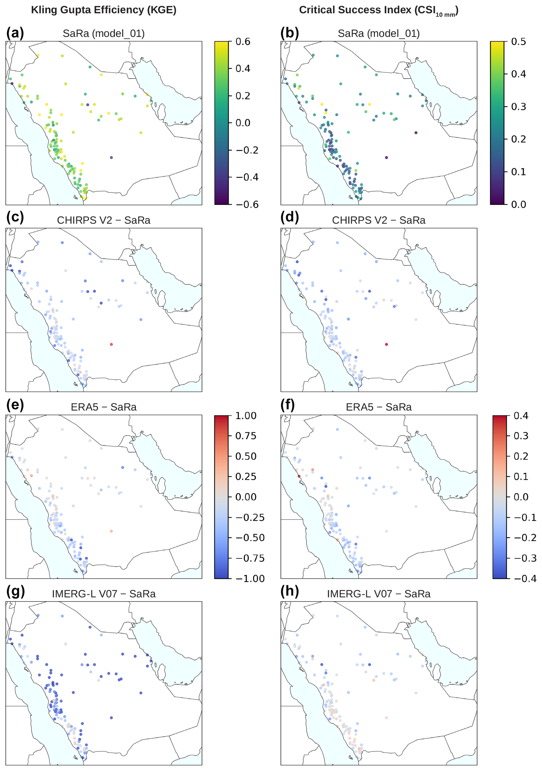
Figure 6 Performance of the primary SaRa ML model (model_01) in terms of (a) Kling–Gupta efficiency (KGE) and (b) detection of P events (CSI_10 mm). (c, e, g) Difference in KGE between model_01 and CHIRPS V2, ERA5, and IMERG-L V07, respectively. (d, f, h) Difference in CSI_10 mm between model_01 and CHIRPS V2, ERA5, and IMERG-L V07, respectively. Each data point represents an independent evaluation gauge (n=119).

Table 5 Spatial Spearman rank correlation coefficients between rain gauge attributes (related to location, climate, and topography; see Table 2) and performance scores (KGE, r_dly, β, etc.; see Sect. 2.6) for six key P products and ML model stacks. The correlations were computed using independent evaluation gauges in Saudi Arabia (n=119).

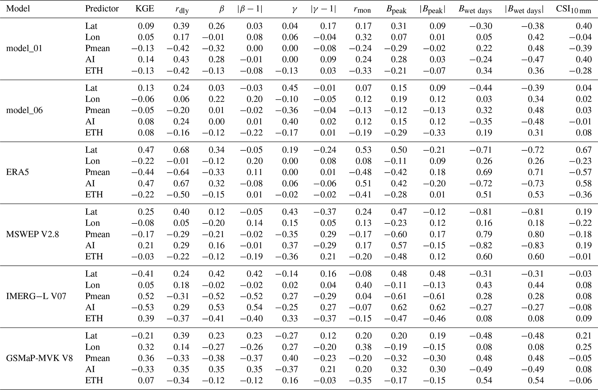
Table 6 Predictor importance (%) for each submodel of model_01. Predictors are ranked in descending order of importance for Submodel 1. ${\widehat{y}}_{\mathrm{Submodel}\mathrm{2}}$ represents the 3-hourly P output of Submodel 2.

To examine whether performance patterns are related to specific climatic or topographic factors, we calculated Spearman rank correlation coefficients between climatic and topographic attributes of the evaluation rain gauges (Table 2) and the performance scores (Sect. 2.6) for SaRa's model_01, SaRa's model_06, MSWEP V2.8, IMERG-L V07, GSMaP MVK V8, and ERA5 (Table 5). Overall, the correlations were slightly weaker for model_01 and model_06 compared to the P products, suggesting more stable performance, which is expected, given that (i) the ML models leverage the complementary strengths of the P predictors and (ii) the climatic and topographic variables were included as predictors in the models.

The metric r_dly, which evaluates the ability of models or products to estimate daily P variability, is primarily sensitive to random errors and less influenced by systematic biases, which are relatively easy to correct. In all models and products, r_dly shows a positive correlation with aridity index (AI), indicating reduced performance in arid regions. This conforms with previous large-scale P product evaluations (e.g., Beck et al., 2017; Sun et al., 2018; Abbas et al., 2025) and reflects the brief, intense, and localized nature of rainfall in such regions. Additionally, r_dly exhibited negative correlations with effective terrain height (ETH) for all models and products, indicating lower performance in the mountainous southwest where orographic P predominates. This is also consistent with other P product evaluations (e.g., Ebert et al., 2007; Derin et al., 2016; Beck et al., 2019a) and reflects the greater heterogeneity of P in regions of complex terrain. Additionally, satellite retrieval of P in mountainous regions is particularly challenging due to the shallow nature of orographic P (Yamamoto et al., 2017; Adhikari and Behrangi, 2022).

Performance metrics related to systematic biases in magnitude (β and B_peak) generally showed negative correlations with mean precipitation (Pmean) and positive correlations with the aridity index (AI). These correlations were particularly strong for IMERG-L V07, suggesting that this product could benefit from bias correction using climate indices.

3.4 Challenges of precipitation estimation in arid regions

Although SaRa outperformed all other P products, its performance metrics might seem underwhelming. For instance, the daily Pearson correlation (r_dly) of 0.50 achieved by model_01 (SaRa's primary model; Table 4) indicates that only 25 % (100×0.50²) of the daily variability in P observations is captured, while other products perform worse. Similarly, a CSI_10 mm of 0.21 suggests a moderate ability to detect P events exceeding 10 mm d⁻¹. These results align with prior large-scale evaluations reporting lower accuracy of P products in arid regions (e.g., Beck et al., 2017; Sun et al., 2018; Abbas et al., 2025), reflecting the inherent challenge of precipitation estimation in these environments.

The challenges in arid regions stem from several key factors:

1. P events in arid regions are typically short-duration, highly intense, and spatially localized, making them difficult to detect with satellites, simulate with models, or measure with gauges. This contrasts with temperate and cold climates, where P events are generally longer-lasting, less intense, and spatially broader (El Kenawy et al., 2019; Ebert et al., 2007).

2. Reanalyses like ERA5 and JRA-3Q and analyses like GDAS are based on numerical weather prediction (NWP) models, which struggle to simulate the complex convective processes prevalent in arid regions, including deep convection initiation, rapid cell dissipation, and the effects of dry boundary layers (Yano et al., 2018; Peters et al., 2019; Lin et al., 2022).

3. Virga P, which evaporates before reaching the ground, adds another layer of complexity. It is estimated to account for nearly half of all events in some arid regions, leading to significant false detections by satellite radiometers (Wang et al., 2018).

4. Errors in gauge measurements – due to wind deflection, evaporation within the gauge, splashing, and wetting losses – can also play a significant role (Ciach, 2003; Daly et al., 2007; Sevruk et al., 2009). In arid regions, higher evaporation rates exacerbate wetting losses, and the sparse, short-lived nature of rainfall events amplifies sampling errors (Villarini et al., 2008).

5. Discrepancies between point measurements from gauges and grid-cell averages derived from satellite or model products also contribute to lower performance scores (Yates et al., 2006; Ensor and Robeson, 2008). In arid regions, this mismatch is likely particularly significant, due to the highly localized nature of P.

6. Time shifts between daily P totals from gauges and satellite or (re)analysis products (Yang et al., 2020; Beck et al., 2019b) further reduce performance scores, especially in arid regions due to the short duration of rainfall events. The boundary between daily totals from satellite or (re)analysis products is midnight UTC, whereas it varies for daily gauge totals depending on regional reporting practices. In Saudi Arabia, the average boundary time was determined to be 05:00 AM UTC (08:00 AM local time; see Sect. 2.6). Consequently, for a brief event of 1 h, there is a $\mathrm{100}\times \mathrm{5}/\mathrm{24}=\mathrm{21}$ % chance that it will be assigned to the “wrong” day.

7. In arid regions, where rainfall is infrequent and therefore measurements are often considered unnecessary, the number of stations is usually limited (Menne et al., 2012; Kidd et al., 2017). As a result, P products may not be evaluated in these areas during development, potentially leading to lower performance.

However, it should be kept in mind that a hypothetical baseline P product predicting only the mean would achieve a KGE of −0.41 (Knoben et al., 2019), making SaRa's model_01 median KGE of 0.36 quite reasonable, situated between this baseline and an (unattainable) perfect score of 1. Furthermore, performance improves markedly when data are averaged over longer periods, as evidenced by the median monthly Pearson correlation (r_mon) of 0.71 for model_01 (Table 4), indicating that more than twice as much variability is captured at the monthly scale compared to the daily scale. Similarly, performance is enhanced at larger spatial scales, for example when computing regional averages or when driving a hydrological model for a catchment. This improved performance reflects the reduced impact of errors due to spatial aggregations within catchments and regions (O and Foelsche, 2019).

3.5 Precipitation climatology and trends in Saudi Arabia

According to the newly developed SaRa P product, the mean annual P for Saudi Arabia during the period 1991–2020 is 54 mm yr⁻¹ (Fig. 7a). However, although SaRa's median β score is 1.03 (Table 4), indicating negligible bias according to this metric, the gauge-based mean (rather than median) P is nonetheless 18 % higher than the SaRa-based mean P across all evaluation gauges, likely reflecting the tendency of ML models to attenuate extremes (see, e.g., He et al., 2016; Ting, 2025). Consequently, an adjusted estimate of $\mathrm{54}\times \mathrm{1.18}=\mathrm{64}$ mm yr⁻¹ may represent the best estimate for mean annual P in Saudi Arabia. This value is significantly lower than the estimate of 102 mm yr⁻¹ for the period 1991–2020 from the Climatic Research Unit (CRU) gridded Time Series (TS) dataset (Harris et al., 2020), as published on the World Bank website (https://climateknowledgeportal.worldbank.org/country/saudi-arabia/climate-data-historical, last access: 18 September 2025). However, the CRU climatology is based on interpolation of a small number of gauges (approximately 10) in Saudi Arabia (New et al., 1999), whereas SaRa was trained using 113 stations in the country. The mean annual P estimate of 84 mm yr⁻¹ from Almazroui (2011), based on TMPA 3B42 (Huffman et al., 2007) bias-corrected using 29 stations, comes closer to our estimate, although it covers a different period (1998–2009).

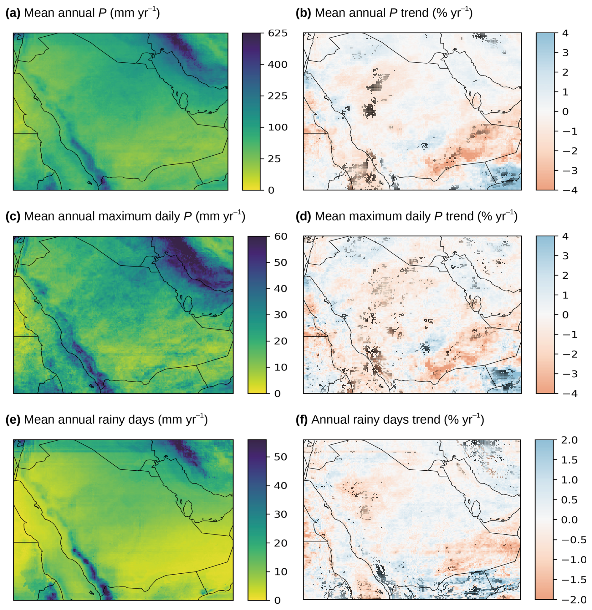
Figure 7 Mean and trend values (1979–2023) based on the new SaRa P product for (a–b) mean annual P, (c–d) annual maximum daily P, and (e–f) annual number of wet days (using a threshold of 0.5 mm d⁻¹). Grid cells with statistically significant trends (p value < 0.05) are marked with black dots. Note that panel (a) uses a non-linear color scale.

In addition to annual totals, SaRa provides insights into P frequency and peak P magnitudes. The average annual maximum daily P in Saudi Arabia is 19 mm d⁻¹ (Fig. 7c). While this value is modest compared to the global best-estimate mean of 56 mm d⁻¹ (from the global gauge-based Precipitation Probability DISTribution – PPDIST – dataset V1.0; Beck et al., 2020), such P extremes can nonetheless cause severe flooding due to the region's low soil infiltration capacity, sparse vegetation, and insufficient flood management infrastructure (Othman et al., 2023). The average annual maximum hourly P is 6.9 mm h⁻¹. On average, Saudi Arabia experiences 10 rainy days per year (defined as days with P≥0.5 mm d⁻¹; Fig. 7e) and 51 rainy hours per year (defined as hours with P≥0.1 mm h⁻¹). For context, the global average number of rainy days per year is 30, based on PPDIST, using the same threshold of 0.5 mm d⁻¹. Across all metrics – mean annual P, P frequency, and P extremes – the highest values occur along the western slopes of the Asir Mountains, where orographic effects enhance P (Hasanean and Almazroui, 2015).

Trend analysis from 1979 to 2023 based on SaRa reveal declines in mean annual P, daily P frequency, and annual maximum daily P at rates of −0.50 % yr⁻¹, −0.11 % yr⁻¹, and −0.58 % yr⁻¹, respectively (see Fig. 7b, d, and f, respectively). Over the 45-year period, these rates correspond to cumulative reductions of −22.5 %, −5.0 %, and −26.1 %, respectively. Our results align with Almazroui (2020), who reported a mean annual P trend of −0.65 % yr⁻¹ during 1978–2019 based on 25 stations in Saudi Arabia. They are also consistent with Munir et al. (2025), who analyzed Standardized Precipitation Index (SPI) time series from 28 stations in Saudi Arabia for 1985–2023, finding negative trends at 16 stations and positive trends at 10. Furthermore, the strong declines observed in southeastern Saudi Arabia (Fig. 7b) align with Patlakas et al. (2021), who analyzed trends for 1986–2015 using a regional atmospheric model. These trends result from multiple factors, including internal climate variability, external natural influences, and human-induced climate change.

However, it is important to note that these trend estimates are mostly statistically insignificant (p value >0.05) and subject to substantial uncertainty due to large interannual variability, as well as considerable errors in gauge, reanalysis, and satellite P estimates (see Sect. 3.4). In addition to random errors, satellite datasets are affected by transitions in data sources and radar sensors used for calibration (e.g., TRMM to GPM circa 2015; see Huffman, 2019), while reanalyses are affected by updates in data assimilation, such as the progressive inclusion of new satellite datasets (e.g., the TOVS to ATOVS transition in 2000), as well as the concatenation of different production streams (Hersbach et al., 2020). These discontinuities propagate through and are reflected in SaRa, contributing to the observed uncertainties and hindering the detection of significant trends. Despite historical declines, future projections from climate models in the sixth phase of the Coupled Model Intercomparison Project (CMIP6) indicate that increases in all three metrics (mean annual P, annual maximum daily P, and annual rainy days) are likely across most regions of Saudi Arabia (Iturbide et al., 2022; IPCC, 2023), highlighting the need and value of data-driven P approaches in resolving potential discrepancies in P distributions and spatio-temporal patterns.

4 Conclusions

The SaRa dataset, a high-resolution, gridded and near-real-time P product, was developed to satisfy the critical need for more accurate and robust P data in the Arabian Peninsula. SaRa offers hourly data at a 0.1° resolution spanning 1979 to the present, with a latency of less than 2 h. The algorithm underpinning the product involves 18 ML model stacks tailored to various P product combinations to ensure optimal performance for each period and location. These models were trained using daily and hourly gauge P observations from across the globe to enhance their accuracy. Our primary findings are summarized as follows:

1. Among the 18 model stacks, model_06, which incorporates four dynamic predictors (ERA5, GDAS, IMERG-L V07, GSMaP-MVK V8), achieved the highest median KGE (0.43). model_01, the primary model spanning the longest period (2000 to 5 d before the present) and incorporating three dynamic predictors (ERA5, IMERG-L V07, GSMaP-MVK V8), also demonstrated strong performance (median KGE of 0.36). Most models showed minimal bias in peak rainfall and wet-day frequency, reinforcing the idea that product performance can be enhanced by leveraging the complementary strengths of diverse P datasets. However, model_05, relying solely on ERA5, performed relatively poorly (median KGE of 0.03) due to significant bias issues, although these were mitigated through harmonization with model_01.

2. We carried out the most comprehensive daily evaluation of gridded P products in the Arabian Peninsula to date. SaRa outperformed all 19 other gridded P products across nearly all 12 performance metrics, achieving a median KGE of 0.36. Notably, it demonstrated superior event detection and lower peak bias compared to state-of-the-art products such as ERA5, JRA-3Q, CMORPH, and IMERG-F V07. Among the evaluated products, microwave-based satellite products generally performed better than infrared-based satellite products and (re)analyses.

3. The spatial performance analysis of SaRa's model_01 across Saudi Arabia, based on KGE and CSI_10 mm metrics, reveals a seemingly random distribution of performance, with clusters of high and low performance influenced by rain gauge errors and scale discrepancies between point and grid measurements. Correlations with climatic and topographic variables suggest relatively stable performance, as these variables were incorporated as predictors in the model. Performance in estimating daily P variability (r_dly) decreases in arid regions and mountainous areas, reflecting challenges with localized, intense rainfall and shallow orographic P.

4. Despite outperforming all other products, SaRa's performance may nonetheless seem somewhat underwhelming, highlighting the inherent difficulty in estimating P in arid regions, where events are typically localized, brief, and intense. For example, SaRa's primary model, model_01, captured only 25 % of daily P variability and the other P products less, possibly due to challenges including virga, short-duration, and highly variable rainfall. However, it is worth noting that achieving perfect scores is impossible due to inherent gauge errors, scale discrepancies, and time shifts in daily accumulations.

5. Mean annual P across Saudi Arabia was estimated as 64 mm yr⁻¹ over the period from 1991–2020, which is significantly lower than prior estimates based solely on rain gauges. Saudi Arabia averages 10 rainy days and 51 rainy hours annually, with higher and more frequent P in the southwestern Asir mountains due to orographic effects. From 1979 to 2023, P trends show a decline in annual totals, frequency, and extremes (up to −26.1 %), driven by climate variability and anthropogenic factors. In contrast to the historical trends, climate projections suggest potential future increases.

Our study addresses the long-standing need for more accurate P estimates and provides a comprehensive evaluation of gridded P products in Saudi Arabia, one of the most arid, water-stressed, and data-sparse regions on Earth. The SaRa dataset, available at https://www.gloh2o.org/sara (last access: 24 September 2025), equips researchers, professionals, and policymakers with the tools needed to tackle pressing environmental and socio-economic challenges in Saudi Arabia and serves not only as a potential framework for filling this data gap in other arid and dryland regions but also as a framework that could be applied globally to develop a consistent long-term dataset. The product delivers a high-resolution, near-real-time resource designed to support a diverse range of applications, including water resource management, hydrological modeling, agricultural planning, disaster risk reduction, and climate studies.

Appendix A: ML model hyperparameters

The hyperparameters used for the RF and XGBoost models are described in Tables A2 and A1, respectively. These hyperparameters were selected to balance model complexity and training time, while also minimizing the risk of overfitting.

Table A1 Hyperparameters for the XGBoost models.

Table A2 Hyperparameters for the RF models.

Appendix B: Performance metrics calculation

The Kling–Gupta efficiency (KGE) is given by

$$\begin{array}{}\text{(B1)}& \mathrm{KGE}=\mathrm{1}-\sqrt{(r-\mathrm{1}{)}^{\mathrm{2}}+(\mathit{\beta }-\mathrm{1}{)}^{\mathrm{2}}+(\mathit{\gamma }-\mathrm{1}{)}^{\mathrm{2}}},\end{array}$$

where r is the Pearson correlation coefficient, β is the overall bias (mean simulated value to mean observed value), and γ is the variance bias (ratio of simulated variance to observed variance).

The Critical Success Index (CSI) is calculated for events exceeding a threshold of 10 mm d⁻¹ as

$$\begin{array}{}\text{(B2)}& \mathrm{CSI}={\displaystyle \frac{H}{H+M+F+{\mathrm{10}}^{-\mathrm{9}}}},\end{array}$$

where H is the number of hits (correctly predicted events), M is the number of misses (events missed by the product), and F is the number of false alarms (incorrectly predicted events). An epsilon value is added to prevent division by zero.

Peak bias at the 99.5th percentile (B_peak; %) is calculated as the percentage difference between the 99.5th percentile of the estimated and observed data:

$$\begin{array}{}\text{(B3)}& B_{\mathrm{peak}}=\mathrm{100}\times {\displaystyle \frac{P_{\mathrm{99.5}}-O_{\mathrm{99.5}}}{O_{\mathrm{99.5}}}},\end{array}$$

where P_99.5 and O_99.5 are the 99.5th percentiles of the estimated and observed values, respectively.

Wet day bias (B_wet days; days) is calculated as the percentage difference in the number of wet days (days exceeding a 0.5 mm d⁻¹ threshold) between simulated and observed data:

$$\begin{array}{}\text{(B4)}& B_{\mathrm{wet}\mathrm{days}}=\mathrm{365.25}\times {\displaystyle \frac{P-O}{N}},\end{array}$$

where P and O are the number of wet days in the estimated and observed time series, respectively, and N is the total number of values.