Combining uncertainty quantification and entropy-inspired concepts into a single objective function for rainfall-runoff model calibration

A novel metric for rainfall-runoff model calibration and performance assessment is proposed. By integrating entropy and mutual information concepts as well as uncertainty quantification through the Brisk Local Uncertainty Estimator for Hydrological Simulations and Predictions (BLUECAT) (likelihood-free approach), the ratio of uncertainty to mutual information (RUMI) offers a robust framework for quantifying the shared information between observed and simulated streamflows. RUMI's capability to calibrate rainfall-runoff models is demonstrated using the GR4J rainfall-runoff model over 99 catchments from various macroclimatic zones, ensuring a comprehensive evaluation. Four additional performance metrics and 50 hydrological signatures are also used for performance assessment. Key findings indicate that RUMI-based simulations provide more consistent and reliable results compared to the traditional Kling–Gupta efficiency (KGE), with improved performance across multiple metrics and reduced variability. Additionally, RUMI includes uncertainty quantification as a core computation step, offering a more holistic view of model performance. This study highlights the potential of RUMI to enhance hydrological modelling through better performance metrics and uncertainty assessment, contributing to more accurate and reliable hydrological predictions.

1 Introduction

1.1 Motivation

Rainfall-runoff models are valuable tools for studying catchment responses to different hydrometeorological inputs and variations in catchment characteristics. Rainfall-runoff modelling considers various modelling choices that can significantly affect modelling results (see, e.g., Alexander et al., 2023; Knoben et al., 2019; Melsen et al., 2019; Mendoza et al., 2016; Thirel et al., 2024; Trotter et al., 2022). Among these, it is worth mentioning the model structure, spatial and temporal discretisation, input data, and calibration strategies. The latter refers not only to the selection period for warm-up, calibration, and validation but also to one or more hydrological variable(s) considered for calibration purposes. The adopted objective function, which quantifies the similarity between observations and simulations, is also critical. Previous studies have highlighted the need for particular objective functions to reproduce case-specific parts of the streamflow time series (see, e.g., Acuña and Pizarro, 2023; Garcia et al., 2017; Mizukami et al., 2019). For instance, if the modeller intends to reproduce high flows (without caring too much about low flows), specific objective functions for high flows are recommended (Hundecha and Bárdossy, 2004; Mizukami et al., 2019). The same can be said for low or middle flows (Garcia et al., 2017).

The Nash–Sutcliffe efficiency (NSE; Nash and Sutcliffe, 1970) and the Kling–Gupta efficiency (KGE; Gupta et al., 2009) are two widely used objective functions for calibration purposes in rainfall-runoff modelling. Despite their popularity, alternatives are available in the literature (see, e.g., without intending to provide a comprehensive list, Kling et al., 2012; Koutsoyiannis, 2025; Onyutha, 2022; Pechlivanidis et al., 2014; Pizarro and Jorquera, 2024; Pool et al., 2018; Tang et al., 2021; Yilmaz et al., 2008). The reader is also referred to the following studies: Bai et al. (2021); Barber et al. (2020); Clark et al. (2021); Jackson et al. (2019); Lamontagne et al. (2020); Lin et al. (2017); Liu (2020); Melsen et al. (2025); Pushpalatha et al. (2012); Vrugt and de Oliveira (2022); and Ye et al. (2021). However, to the best of our knowledge, only a small number of objective functions – considering uncertainty quantification explicitly as a core step in its computation – are available (even though hydrology has witnessed a growing emphasis on uncertainty quantification, driven by the need to enhance our understanding of catchments and to provide decision-makers with accurate model predictions). Advancements in the direction of proposing a novel and easy-to-use objective function that considers uncertainty quantification in its formulation is the primary goal of this paper.

1.2 Uncertainty quantification methods

Various methodologies aimed at better treating uncertainty are available, each differing in their underlying assumptions, mathematical rigour, and treatment of error sources (see, e.g., Beven, 2018; Blazkova and Beven, 2002, 2004; Krzysztofowicz, 2002). Among these approaches (see Gupta and Govindaraju, 2023, for a recent review), we can mention the additive Gaussian and generalised-Gaussian process, the inference in the spectral domain, the time-varying model parameters, and multi-model ensemble methods. Additionally, two philosophies for uncertainty analysis are widely recognised, following formal and informal Bayesian methods (Kennedy and O'Hagan, 2001; Kuczera et al., 2006).

Formal Bayesian methods offer robust frameworks for uncertainty estimation, but they come with their own challenges. Identifying a suitable likelihood function for hydrological models involves careful assumptions that must be transparent and understandable to end users (Beven, 2024; Vrugt et al., 2022). Statistical analysis of model errors and likelihood-free approaches have also been proposed. For example, Montanari and Koutsoyiannis (2012) proposed converting deterministic models into stochastic predictors by fitting model errors with meta-Gaussian probability distributions. Similarly, Sikorska et al. (2015) proposed the nearest neighbouring method to estimate the conditional probability distribution of the error. More recently, Koutsoyiannis and Montanari (2022a) introduced a simple method to simulate stochastic runoff responses called the Brisk Local Uncertainty Estimator for Hydrological Simulations and Predictions (BLUECAT). BLUECAT is a likelihood-free approach that relies on data only. BLUECAT has recently been applied coupled with climate extrapolations (Koutsoyiannis and Montanari, 2022b), rainfall-runoff modelling in a variety of different hydroclimatic conditions (Jorquera and Pizarro, 2023), and comparisons with machine-learning methods (Auer et al., 2024; Rozos et al., 2022).

Informal Bayesian methods are more flexible, but they lack statistical rigour. A notable example of a relatively simple approach is the generalised likelihood uncertainty estimation (GLUE) method introduced by Beven and Binley (1992). GLUE operates within the framework of Monte Carlo analysis coupled with Bayesian or fuzzy uncertainty estimation and propagation. Since its introduction, GLUE has seen widespread application across various fields, including rainfall-runoff modelling (among others). Its popularity is mainly due to its conceptual simplicity and ease of implementation. It can account for all causes of uncertainty, either explicitly or implicitly, and allows for evaluating multiple competing modelling approaches, embracing the concept of equifinality (Beven, 1993). However, GLUE has faced criticism in terms of the subjective decisions required in its application and how these affect prediction limits (informal likelihood function, lack of maximum likelihood parameter estimation, and omission of explicit model error consideration). This subjectivity might lead to not being formally Bayesian (for that reason, GLUE includes the term “generalised” in its name). Proponents of GLUE argue that it is a practical methodology for assessing uncertainty in non-ideal cases (Beven, 2006), while critics advocate for coherent probabilistic approaches. This ongoing debate underscores the need to establish common ground between these perspectives. Under various conditions, both Bayesian and informal Bayesian methods can yield similar estimates of predictive uncertainty. Building on previous work (see, e.g., Blasone et al., 2008), researchers have compared GLUE with formal Bayesian approaches. In this regard, both formal Bayesian approaches as well as GLUE can be used with advanced Monte Carlo Markov chain (MCMC) schemes such as the DiffeRential Evolution Adaptive Metropolis (DREAM, Vrugt et al., 2008). It is important to note that defining likelihood functions and searching the solution space during calibration are two independent issues. One way to get around these problems relies on the limits of acceptability that are typically used (but not mandatory) with GLUE (see, e.g., Beven et al., 2024; Beven and Lane, 2022; Freer et al., 2004; Page et al., 2023; Vrugt and Beven, 2018), involving more thoughtful decisions about the data (although still with subjectivity). Additionally, studies have addressed these questions by assessing the uncertainty in synthetic river flow data using GLUE (see, e.g., Montanari, 2005) and introducing open-source software packages such as the CREDIBLE uncertainty estimation toolbox (CURE; Page et al., 2023), coded in MATLAB (https://www.lancaster.ac.uk/lec/sites/qnfm/credible/default.htm, last access: 3 December 2024). CURE includes several methods, among them the forward uncertainty estimation, GLUE, and Bayesian statistical methods.

In addition to these methods, information theory offers valuable tools for quantifying information in hydrological models. Shannon's (1948) seminal work on information theory introduced measures such as Shannon entropy, which quantifies the expected surprise (or information) in a sample from a distribution of states. Shannon entropy can be extended to joint distributions of multiple variables, including conditional dependencies. In hydrology, Shannon entropy and mutual information have been used to assess the uncertainty in discharge predictions, as demonstrated by Amorocho and Espildora (1973) and Chapman (1986). More recently, Weijs et al. (2010a, b), Gong et al. (2013, 2014), Pechlivanidis et al. (2014, 2016), and Ruddell et al. (2019) used information-theoretic objective functions for model evaluation. Despite the challenges associated with accounting for uncertainties and statistical dependencies in time series data, information-theoretic objective functions have proven valuable for streamflow simulations, complementing traditional measures such as the Nash–Sutcliffe efficiency (NSE; Nash and Sutcliffe 1970) and the Kling–Gupta efficiency (KGE; Gupta et al., 2009; Kling et al., 2012).

1.3 Paper's goals

In this work, we study the combination of likelihood-free (BLUECAT) and information theory approaches for rainfall-runoff modelling over 99 catchments having different hydroclimatic contexts, with the intention to quantify and reduce uncertainty in hydrological predictions. The ratio of uncertainty to mutual information (RUMI) is proposed as a dimensionless metric to be adopted as an objective function for calibration purposes. The target aligns with the 20th of the 23 unsolved problems in hydrology (20. How can we disentangle and reduce model structural/parameter/input uncertainty in hydrological prediction?, Blöschl et al., 2019). In detail, the following questions are herein addressed:

• a.

  How can the calibration of deterministic model parameters be improved by using a stochastic formulation of the deterministic model?

• b.

  How can uncertainty resulting from the final stochastic model be incorporated into the calibration process of the deterministic model?

This paper is organised as follows: Sect. 2 presents the used database (catchment properties and data availability), rainfall-runoff model description, and calibration strategies. Section 3 shows the calibration and validation results of RUMI-based simulations (as well as KGE-based ones). Daily runoff simulations and hydrological signatures are considered. Strengths and limitations are discussed in Sect. 4, and conclusions are drawn at the end.

2 Methods

2.1 Data

Ninety-nine catchments were selected from the CAMELS-CL database (Alvarez-Garreton et al., 2018a) to ensure that only catchments with near-natural hydrological regimes were included (see Fig. 1 for location and chosen catchment characteristics; five macroclimatic zones are covered). The latter was achieved through eight specific criteria: first, the daily discharge time series, though possibly non-consecutive, had to have less than 25 % missing data for the period 1990–2018. Additionally, catchments with large dams were excluded (big_dam = 0). Moreover, catchments with more than 10 % of discharge allocated to consumptive uses were excluded (i.e. interv_degree < 0.1 to be considered). Catchments with glacier cover higher than 5 % were also excluded (i.e. lc_glacier < 5 % to be considered). Furthermore, the selected catchments had less than 5 % of their area classified as urban (imp_frac < 5 %), and irrigation abstractions did not exceed 20 % (crop_frac < 20 %). Areas with forest plantations covering more than 20 % of the catchment area were also excluded (fp_frac < 20 %). Finally, catchments showing signs of artificial regulation in their hydrographs were removed. It is worth mentioning that after each criterion mentioned above, there is a description in the parentheses that follows the CAMELS-CL nomenclature. For instance, glacier cover is catalogued as “lc_glacier”, and large dams, as “big_dam”.

The chosen catchments have diverse characteristics, reflecting significant variability. For instance, the smallest catchment has a size of 35 km², whereas the largest one has a size of 11 137 km² (median catchment size is 672 km³). In terms of mean annual precipitation, it ranges from 94 to 3660 mm yr⁻¹ (median value of 1393 mm yr⁻¹). The aridity index also covers a wide spectrum of values, ranging from 0.3 (southern Chile) to 31.6 (northern Chile). Its median is 0.69. In terms of mean elevations, they range between 118 (western, Pacific Ocean) and 4270 (eastern, Andes Mountains) metres above sea level (m a.s.l.). They have a median elevation of 1052 m a.s.l. In terms of seasonality, winter rainfall predominates, with a few exceptions in northern catchments, where precipitation is concentrated during the summer (Garreaud, 2009). Additionally, precipitation usually increases from north to south, while temperatures decrease (Sarricolea et al., 2017). Daily precipitation and potential evapotranspiration data from the CAMELS-CL database were used, with the primary output being simulated daily streamflow. The analysis focuses on the period from 1990 to 2018, with a warm-up phase from 1990 to 1992, a calibration phase from 1992 to 2005, and a validation phase from 2005 to 2018.

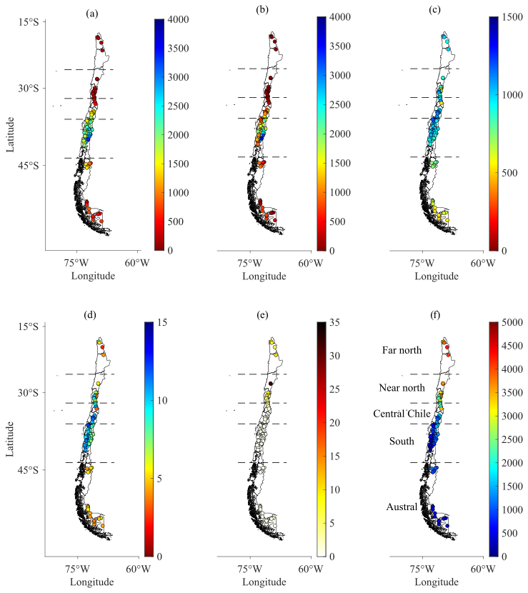
Figure 1 Locations and characteristics of analysed catchments. Coloured dots represent the catchment outlet locations. Five zones are explicitly presented (labelled in (f)) to highlight differences in the catchment climatic characteristics. From (a) to (c), mean annual precipitation, runoff, and potential evapotranspiration (all of them in [mm]). (d) Mean annual temperature in [°C], (e) aridity index (dimensionless), and (f) catchment outlet elevations in [m].

2.2 Rainfall-runoff model

The Modular Assessment of Rainfall-Runoff Models Toolbox (MARRMoT; Knoben et al., 2019; Trotter et al., 2022) was selected due to its open-source feature and modular structure. Implemented in MATLAB, MARRMoT offers a suite of 47 lumped models for simulating rainfall-runoff processes.

MARRMoT version 2.1.2, with the GR4J model, was employed for this study. The GR4J model has four parameters and two storage components. Its primary purpose is to represent processes such as vegetation interception, time delays within the catchment, and water exchange with neighbouring catchments (for detailed information of the GR4J model, see Perrin et al., 2003, and the official website of the developers: https://webgr.inrae.fr/eng/tools/hydrological-models, last access: 22 September 2025). MARRMoT's nomenclature for rainfall-runoff models is “m_XX_YY_ZZp_KKs”, where XX is the number of the models within MARRMoT, YY is the model name, ZZ is the number of parameters, and KK is the number of storages. As a consequence, the GR4J model following the MARRMoT nomenclature is “m_07_gr4j_4p_2s”. For a comprehensive description, readers are directed to the MARRMoT user manual, available at https://github.com/wknoben/MARRMoT/blob/master/MARRMoT/User%20manual/v2.-%20User%20manual%20-%20Appendices.pdf (last access: 22 September 2025).

2.3 Ratio of uncertainty to mutual information (RUMI) objective function

The primary goal of this paper is to introduce a new objective function that considers uncertainty quantification in its formulation; therefore, it is expected to minimise this quantified uncertainty in calibration. As a consequence, the ratio of uncertainty to mutual information (RUMI) is proposed (see Eq. 4 for the mathematical expression and Fig. 3 for the RUMI computation flowchart). RUMI relies on BLUECAT and mutual information (entropy-based computation), which are briefly introduced in the following.

Koutsoyiannis and Montanari (2022a) proposed BLUECAT with the intention of transforming a deterministic prediction model into a stochastic one. BLUECAT's predecessor was introduced by Montanari and Koutsoyiannis (2012). BLUECAT transforms deterministic simulations into stochastic simulations (with confidence bands). Unlike deterministic predictions, the confidence band represents a range of possible outcomes, allowing the stochastic result to be considered as a representative value of the sample (such as the mean or median). It is worth mentioning that uncertainty can be quantified as well. We use BLUECAT to transform deterministic rainfall-runoff simulations to stochastic ones to consider uncertainty quantification in model calibration.

BLUECAT's flowchart starts with a deterministic simulation and identifies the simulated variable (streamflow in our case) at each time point (see Fig. 2 for a conceptual illustration of the BLUECAT methodology). For each point, a sample is established comprising neighbouring simulated river flows (in magnitude), defined by m₁ flows smaller and m₂ flows larger than the point's discharge, both with the smallest differences. m₁ and m₂ were set at 20 because the lowest and highest quantiles can be empirically estimated. The observed data corresponding to these simulated flows form a sample of streamflow values. The latter occurs at each time point. An empirical distribution function of this sample is then used to estimate uncertainty for a given confidence level, using the mean or median as representative results of the stochastic simulation. Alternative methods, such as the ones using a theoretical probability distribution, can also manage the sample (e.g. Pareto–Burr–Feller with knowable moments).

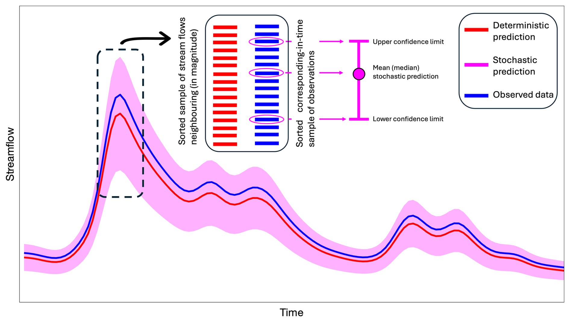
Figure 2 Conceptual illustration of the BLUECAT methodology. Blue represents observed (streamflow) data, whereas red and pink denote deterministic and stochastic predictions, respectively.

In this work, BLUECAT is used with empirical computations with the intention of avoiding any additional assumption. It is worth mentioning that BLUECAT allows uncertainty quantification through an uncertainty measure. Montanari and Koutsoyiannis (2025) proposed four measures based on the distance between the confidence bands, for a given significance level, and the mean value of the prediction. BLUECAT was originally implemented in R (coupled with the HYMOD rainfall-runoff model; Koutsoyiannis and Montanari, 2022a), and Montanari and Koutsoyiannis (2025) recently made available BLUECAT with multi-model usage in R and Python. Codes in MATLAB are also available (see Jorquera and Pizarro, 2023).

In information theory, the entropy of a random variable is a measure of its uncertainty or the measure of the information amount required, on average, to describe the random variable itself (Thomas and Joy, 2006). The amount of information one random variable contains about another random variable is usually defined as mutual information (MI). MI is, indeed, the reduction of one random variable uncertainty due to the knowledge of the other. MI can be defined as a function of marginal $\left(H\left(\underset{\mathrm{¯}}{Y}\right)\right)$ and conditional $\left(H(\underset{\mathrm{¯}}{Y}/\underset{\mathrm{¯}}{X})\right)$ entropies:

$$\begin{array}{}\text{(1)}& \mathrm{MI}(\underset{\mathrm{¯}}{Y},\underset{\mathrm{¯}}{X})=H\left(\underset{\mathrm{¯}}{Y}\right)-H(\underset{\mathrm{¯}}{Y}/\underset{\mathrm{¯}}{X}),\end{array}$$

where $H\left(\underset{\mathrm{¯}}{Y}\right)=-E\left[\log \left(p\left(Y\right)\right)\right]$, $H\left(\underset{\mathrm{¯}}{Y}/\underset{\mathrm{¯}}{X}\right)=-E\left[\log \left(p\left(Y/X\right)\right)\right]$, p(α) is the probability mass function of a random variable $\underset{\mathrm{¯}}{\mathit{\alpha }}$ (or the probability density if the variable is of the continuous type), and E[] denotes expectation. Note that random variables are underlined, following the Dutch convention (Hemelrijk, 1966).

Additionally, the normalised mutual information (also called the uncertainty coefficient, entropy coefficient, or Theil's U) can be computed as:

$$\begin{array}{}\text{(2)}& U\left(\underset{\mathrm{¯}}{Y},\underset{\mathrm{¯}}{X}\right)={\displaystyle \frac{\mathrm{MI}\left(\underset{\mathrm{¯}}{Y},\underset{\mathrm{¯}}{X}\right)}{H\left(\underset{\mathrm{¯}}{Y}\right)}}={\displaystyle \frac{H\left(\underset{\mathrm{¯}}{Y}\right)-H(\underset{\mathrm{¯}}{Y}/\underset{\mathrm{¯}}{X})}{H\left(\underset{\mathrm{¯}}{Y}\right)}}.\end{array}$$

Taking $\underset{\mathrm{¯}}{Y}$ as the observed streamflow $\left(\underset{\mathrm{¯}}{Q_{\mathrm{obs}}}\right)$ and $\underset{\mathrm{¯}}{X}$ as the simulated one with BLUECAT ($\underset{\mathrm{¯}}{Q_{\mathrm{sim}}}$, given by the mean value of the distribution of the predictand), $U\left(\underset{\mathrm{¯}}{Y},\underset{\mathrm{¯}}{X}\right)=U\left(\underset{\mathrm{¯}}{Q_{\mathrm{obs}}},\underset{\mathrm{¯}}{Q_{\mathrm{sim}}}\right)$ represents the normalised amount of information that $\underset{\mathrm{¯}}{Q_{\mathrm{sim}}}$ contains about $\underset{\mathrm{¯}}{Q_{\mathrm{obs}}}$. Note that $\underset{\mathrm{¯}}{Q_{\mathrm{sim}}}$ can also be estimated by the median value of the distribution of the predictand (or another quantile). The decision to use the mean value relies on Jorquera and Pizarro (2023) results that showed higher KGE values using the mean rather than the median value for all analysed catchments. Additionally, and with the intention to avoid any additional assumption, marginal and conditional entropies are computed empirically with bins.

Furthermore, an uncertainty measure (in line with the Jorquera and Pizarro (2023) and Montanari and Koutsoyiannis (2025) uncertainty quantification proposal) of the stochastic model computed with BLUECAT can be defined as the width of the confidence limits divided by its mean value and averaged over the whole simulation period, i.e.:

$$\begin{array}{}\text{(3)}& u=\sum _{\mathit{\tau }=\mathrm{1}}^n{\displaystyle \frac{\mathrm{1}}{n}}\left|{\displaystyle \frac{Q_{\mathit{\tau },\mathrm{u}}-Q_{\mathit{\tau },\mathrm{l}}}{Q_{\mathit{\tau },\mathrm{sim}}}}\right|,\end{array}$$

where $Q_{\mathit{\tau },\mathrm{u}}-Q_{\mathit{\tau },\mathrm{l}}$ are the upper and lower confidence limits for the streamflow stochastic prediction at time step τ, Q_τ,sim is its mean value at time step τ, and n is the total number of time steps.

Notice that both u and $U\left(\underset{\mathrm{¯}}{Q_{\mathrm{obs}}},\underset{\mathrm{¯}}{Q_{\mathrm{sim}}}\right)$ are dimensionless quantities, and, in ideal conditions, it is desirable that u is minimised (i.e. low uncertainty), whereas $U\left(\underset{\mathrm{¯}}{Q_{\mathrm{obs}}},\underset{\mathrm{¯}}{Q_{\mathrm{sim}}}\right)$ is maximised (i.e. high mutual information between simulated and observed streamflows). Therefore, the ratio between u and $U\left(\underset{\mathrm{¯}}{Q_{\mathrm{obs}}},\underset{\mathrm{¯}}{Q_{\mathrm{sim}}}\right)$ gives a measure of the simulation performance. It is worth mentioning that the advantage of taking this ratio does rely not only on a mathematical functionality (i.e. the ratio should be minimised in calibration) but also on the fact that it is possible to have narrow confidence limits (i.e. low uncertainty) with a bad performance between the stochastic model predictand and observed values (i.e. low mutual information; see Fig. 3a). Additionally, it is also possible to have high mutual information (stochastic model predictand close to observed values) but with high uncertainty, as shown in Fig. 3b. Therefore, the reason for taking the ratio is 2-fold: (i) mathematical desire (i.e. optimisation) and (ii) deductive conceptual reasoning. As a consequence, and with the intention to provide a metric ranging between 0 and 1, the ratio of uncertainty to mutual information (RUMI) is presented as follows:

$$\begin{array}{}\text{(4)}& \mathrm{RUMI}={\displaystyle \frac{\mathrm{1}}{\mathrm{1}+\mathit{\varphi }}}={\displaystyle \frac{\mathrm{1}}{\mathrm{1}+\frac{u}{U\left(\underset{\mathrm{¯}}{Q_{\mathrm{obs}}},\underset{\mathrm{¯}}{Q_{\mathrm{sim}}}\right)}}}.\end{array}$$

Notice that RUMI follows common-efficiency notions (i.e. perfect simulation means the highest metric value). Figure 3d shows the core steps of the RUMI computation, whereas the codes for RUMI in MATLAB and R are also made available (see “Code and data availability” statement).

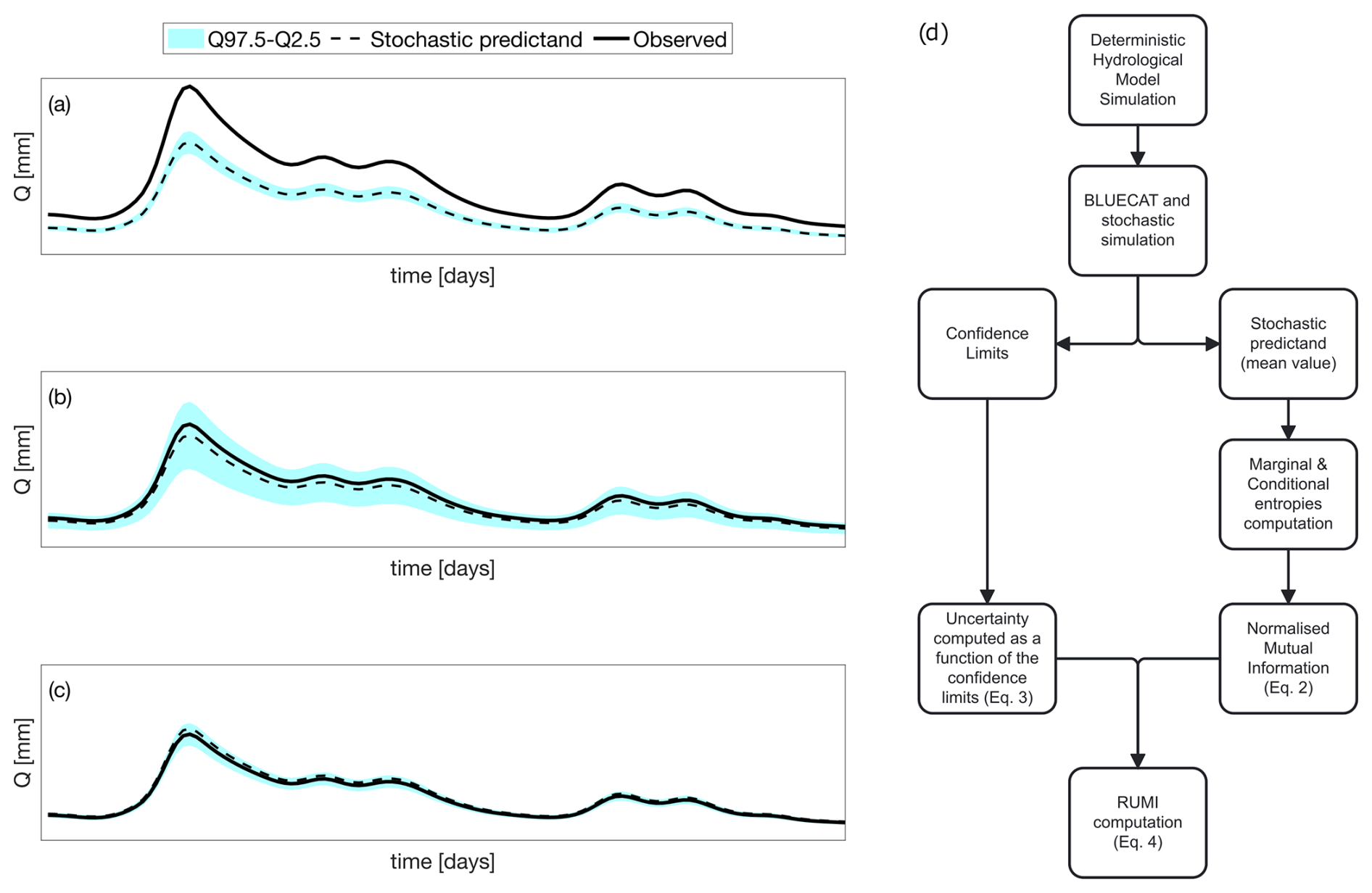
Figure 3 Illustration of possible modelling scenarios: (a) low uncertainty and low mutual information (i.e. low RUMI value); (b) high uncertainty and high mutual information (i.e. low RUMI value); and (c) low uncertainty and high mutual information (i.e. high RUMI value). (d) Flowchart of the RUMI computation. Marginal and conditional entropies are computed empirically with bins. The filled cyan band is the area between the 97.5th and 2.5th percentiles of the simulation estimated by BLUECAT.

2.4 Calibration and validation strategies

The GR4J rainfall-runoff model calibration was conducted using the covariance matrix adaptation evolution strategy (CMA-ES) algorithm (Hansen et al., 2003; Hansen and Ostermeier, 1996). Catchments were calibrated with two different objective functions: KGE and RUMI. KGE (Kling et al., 2012) – computed in this study with Eq. (5) – is the modified version of the KGE proposed initially by Gupta et al. (2009):

$$\begin{array}{}\text{(5)}& \mathrm{KGE}=\mathrm{1}-\sqrt{{\left({\displaystyle \frac{{\mathit{\mu }}_{\mathrm{s}}}{{\mathit{\mu }}_{\mathrm{o}}}}-\mathrm{1}\right)}^{\mathrm{2}}+{\left({\displaystyle \frac{\left({\mathit{\sigma }}_{\mathrm{s}}/{\mathit{\mu }}_{\mathrm{s}}\right)}{\left({\mathit{\sigma }}_{\mathrm{o}}/{\mathit{\mu }}_{\mathrm{o}}\right)}}-\mathrm{1}\right)}^{\mathrm{2}}+{\left(\mathit{\rho }-\mathrm{1}\right)}^{\mathrm{2}}},\end{array}$$

where μ_s is the mean value of deterministic streamflow simulations; μ_o is the mean value of streamflow observations; σ_s is the standard deviation of deterministic streamflow simulations; σ_o is the standard deviation of streamflow observations; and ρ is the Pearson correlation coefficient between the observed and deterministic simulations of streamflow.

Four additional metrics were used to assess the performance of results: (i) Nash–Sutcliffe efficiency (NSE); (ii) KGE knowable moments (KGEkm; Pizarro and Jorquera, 2024); (iii) normalised root mean squared error (NRMSE); and (iv) mean absolute relative error (MARE). Equations for NSE, KGEkm, NRMSE, and MARE are presented from Eqs. (6) to (9):

$$\begin{array}{}\text{(6)}& {\displaystyle }\mathrm{NSE}=\mathrm{1}-{\displaystyle \frac{{\sum }_{i=\mathrm{1}}^n{\left(O_i-S_i\right)}^{\mathrm{2}}}{{\sum }_{i=\mathrm{1}}^n{\left(O_i-{\mathit{\mu }}_{\mathrm{o}}\right)}^{\mathrm{2}}}},\text{(7)}& {\displaystyle }\begin{array}{rl}& \mathrm{KGEkm}=\mathrm{1}-\\ & \sqrt{{\left({\displaystyle \frac{K_{{\mathrm{1}}_{\mathrm{s}}}}{K_{{\mathrm{1}}_{\mathrm{o}}}}}-\mathrm{1}\right)}^{\mathrm{2}}+{\left({\displaystyle \frac{\left({\sqrt{K}}_{{\mathrm{2}}_{\mathrm{s}}}/K_{{\mathrm{1}}_{\mathrm{s}}}\right)}{\left({\sqrt{K}}_{{\mathrm{2}}_{\mathrm{o}}}/K_{{\mathrm{1}}_{\mathrm{o}}}\right)}}-\mathrm{1}\right)}^{\mathrm{2}}+{\left(\mathit{\rho }-\mathrm{1}\right)}^{\mathrm{2}}},\end{array}\text{(8)}& {\displaystyle }\mathrm{NRMSE}={\displaystyle \frac{\sqrt{\frac{\mathrm{1}}{n}\left({\sum }_{i=\mathrm{1}}^n{\left(S_i-O_i\right)}^{\mathrm{2}}\right)}}{max\left(O\right)-min\left(O\right)}},\text{(9)}& {\displaystyle }\mathrm{MARE}={\displaystyle \frac{{\sum }_{i=\mathrm{1}}^n\left|\frac{\left(S_i-O_i\right)}{O_i}\right|}{n}},\end{array}$$

where $K_{{\mathrm{1}}_{\mathrm{s}}}$ and $K_{{\mathrm{1}}_{\mathrm{o}}}$ are the first knowable moments of the simulated and observed streamflow time series and $K_{{\mathrm{2}}_{\mathrm{s}}}$ and $K_{{\mathrm{2}}_{\mathrm{o}}}$ are dispersions relying on the second knowable moments of the simulated and observed streamflow time series. Notice that the square operator in K₂ is not necessary in Eq. (7) but intentionally used to be in line with classical statistics and KGE formulation (see Eq. 5). S and O denote simulated and observed streamflow time series, respectively. n is the length of the analysed period (at daily scale). RMSE, NRMSE, and MARE have 0 as the perfect ideal value, whereas their values range from 0 to positive infinity. NSE and KGEkm have a range from minus infinity to 1, with 1 being the ideal value.

Additionally, and with a particular focus on different runoff characteristics, 50 hydrological signatures were computed. Observed runoff, simulations with the model calibrated with KGE, and simulations with the model calibrated with RUMI were considered. Hydrological signatures were computed with the Toolbox for Streamflow Signatures in Hydrology (TOSSH; Gnann et al., 2021). Table 1 shows the 50 computed signatures.

Table 1 Fifty hydrological signatures computed with the Toolbox for Streamflow Signatures in Hydrology (TOSSH). The computed hydrological signatures follow TOSSH nomenclature (e.g. TotalRR is the total runoff ratio). A description of the signatures is also included.

3 Results

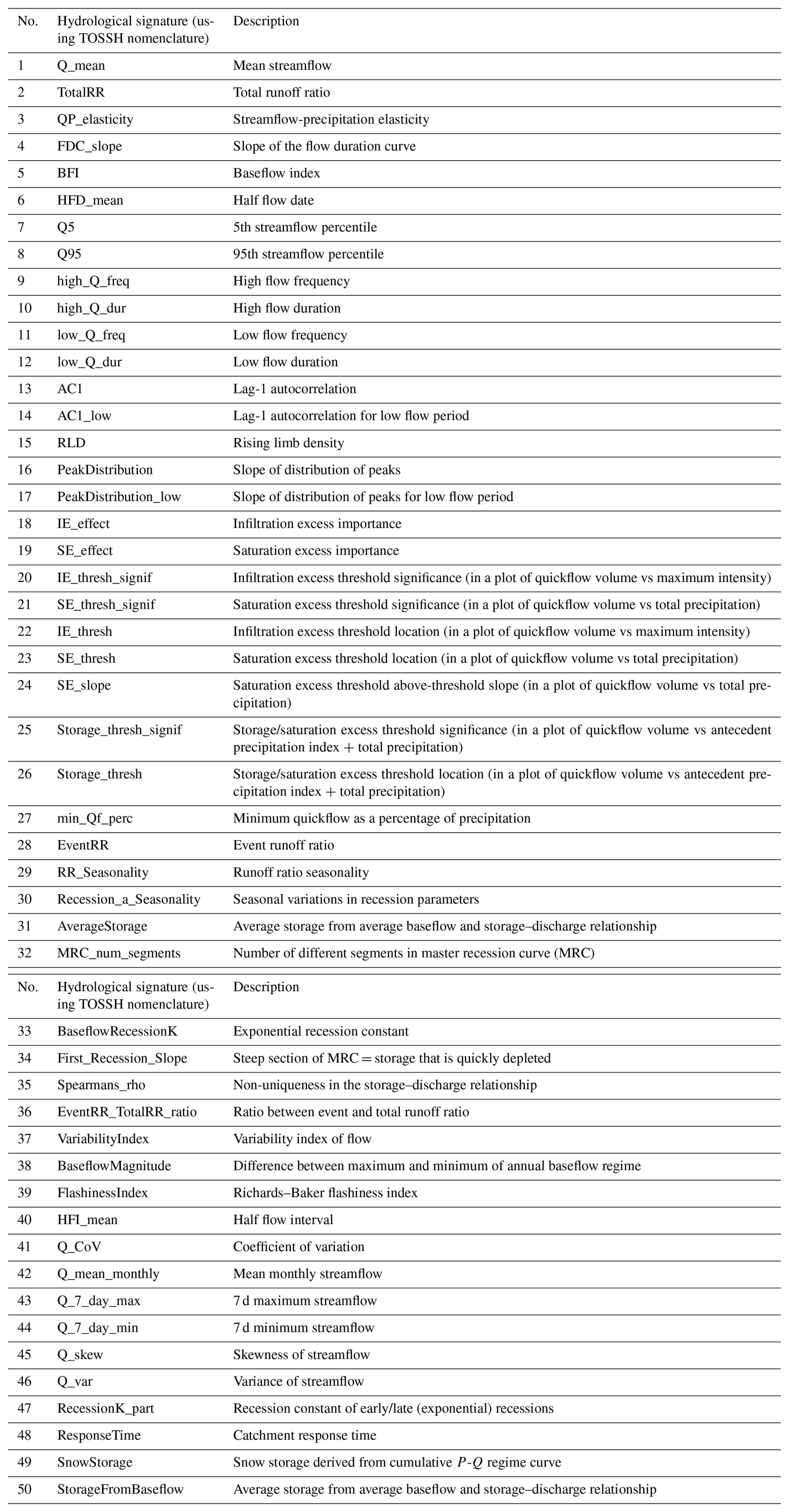
Figure 4 shows a graphical example of RUMI-based hydrological modelling of two of the catchments in calibration (Fig. 4a, catchment number: 8123001) and validation (Fig. 4b, catchment number: 9437002) over the years 1996 and 2016, respectively. Additionally, it shows observed and simulated streamflows, which were calibrated with KGE (red continuous line) and RUMI (blue continuous line is the mean of the stochastic simulation). The 97.5th and 2.5th percentiles (computed with BLUECAT and RUMI) are shown with a violet band. Figure 4a.2 and 4b.2 show observed and simulated streamflows over the complete period of analysis (the performance of KGE-based simulations was 0.89 (0.80) and 0.95 (0.91) in calibration (validation), and the performance of RUMI-based simulations was 0.27 (0.20) and 0.46 (0.48) in calibration (validation), respectively). Note that the observed streamflow was between the 97.5th and 2.5th percentiles (i.e. the violet band) all the time except for 4.93 % and 0.19 % of the time, where higher and lower observed streamflow, respectively, were presented (see, e.g., one event in June 1996 in Fig. 3a and one event in July 2016 in Fig. 3b).

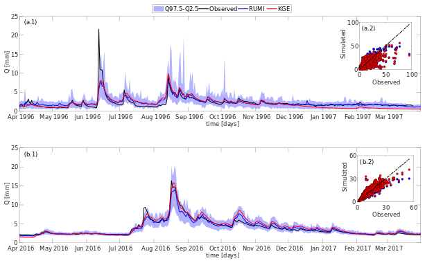
Figure 4 Observed and simulated streamflows for the hydrological years 1996–1997 (a) and 2016–2017 (b). (a.1) Catchment ID: 8123001 in calibration; (b.1) catchment ID: 9437002 in validation. Black: observed streamflow; red: simulated by the deterministic model calibrated with KGE; blue: simulated with the model calibrated with RUMI (mean stochastic simulation). The filled violet band is the area between the 97.5th and 2.5th percentiles of the simulation estimated by BLUECAT. The dashed line represents perfect agreement between the observed and simulated streamflows.

In terms of other performance metrics, Fig. 5 shows NSE (a.1, b.1), KGEkm (a.2, b.2), NRMSE (a.3, b.3), and MARE (a.4, b.4) in calibration (a.1, a.2, a.3, a.4) and validation (b.1, b.2, b.3, b.4). Red markers are outliers, and grey dots represent the mean values (as a function of RUMI- and KGE-based simulations), which are linked with a grey line.

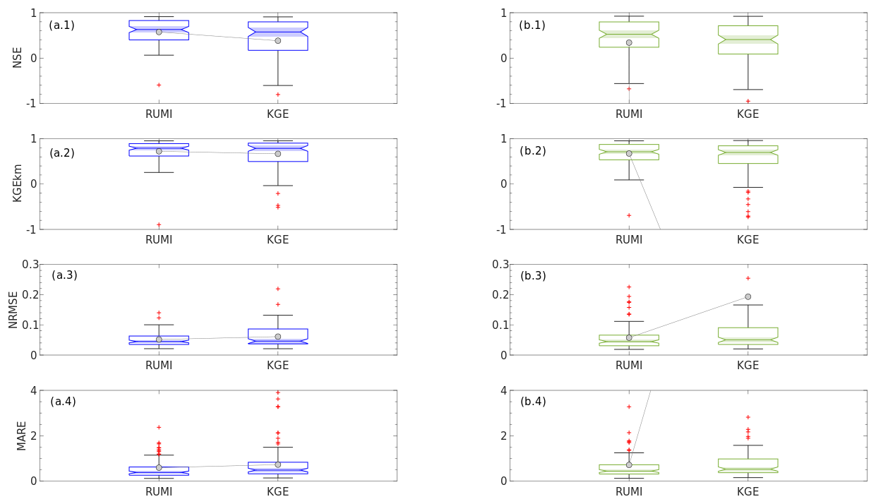
Figure 5 Performance metrics in calibration (a.1, a.2, a.3, a.4) and validation (b.1, b.2, b.3, b.4). Red markers denote outliers. Grey dots represent the mean values computed with RUMI and KGE, which are linked by grey lines. Note that the y-axis limits are truncated for visualisation purposes.

Remarkably, the RUMI-based simulations outperform the KGE-based ones in both calibration and validation and for the four performance metrics analysed. The latter is in terms of variability (e.g. the interquartile range – IQR), median of boxplots, and number of outliers for both the calibration and validation periods. Table 2 summarises the four considered performance metrics in terms of (a) calibration and validation; (b) RUMI and KGE; and (c) minimum, maximum, median, IQR, and mean values.

Table 2 Statistical summary of the boxplot results (see also Fig. 5).

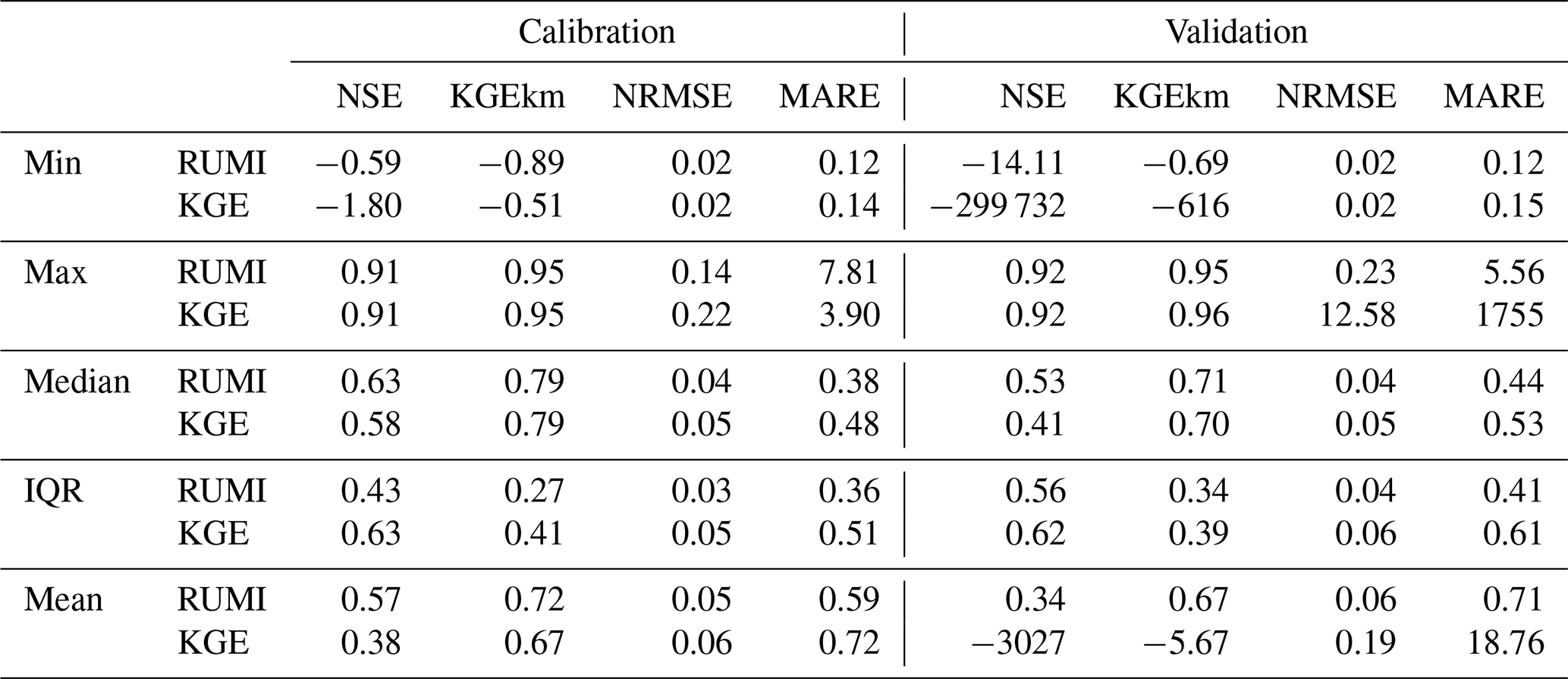
Based on Fig. 4 and Table 2, the RUMI-based simulations showed more stable and consistent performance than KGE in the calibration and validation phases. While KGE can achieve high accuracy (see, e.g., the maximum value of NSE for RUMI and KGE), it exhibits more variability and more extreme outliers (see, e.g., the minimum values of NSE: −14.11 vs −299 732 for RUMI and KGE; the mean values of NSE: 0.34 vs −3027 for RUMI and KGE; the minimum values of KGEkm: −0.69 vs −616 for RUMI and KGE; the maximum values of NRMSE: 0.23 vs 12.58 for RUMI and KGE; and the maximum values of MARE: 5.56 vs 1755 for RUMI and KGE). The latter, particularly during validation, indicates a lack of robustness. On the other hand, RUMI presented lower variability, more consistent results, and the opportunity to consider the confidence intervals in calibration.

Table 3 shows the Pearson's correlation coefficient for the 50 computed hydrological signatures considering observed and simulated streamflow data (“Obs vs KGE” means the Pearson's correlation coefficient using observed and simulated-with-KGE streamflows to compute any hydrological signature; “Obs vs RUMI” means the Pearson's correlation coefficient using observed and simulated-with-RUMI streamflows to compute any hydrological signature). On average, RUMI outperforms the KGE-based simulations (average values: 0.72 vs 0.48; minimum and maximum values: −0.07 vs −0.10 and 1.00 vs 0.96, respectively). The RUMI-based simulations outperform the KGE-based ones by 82 % for the considered hydrologic signatures. Figure 6 shows four examples of this comparison in terms of the runoff ratio (TotalRR; Fig. 6a), streamflow-precipitation elasticity (QP_elasticity; Fig. 6b), 5th flow percentile of the streamflow (Q5; Fig. 6c), and 95th flow percentile of the streamflow (Q95; Fig. 6d). The colours of the dots are related to the five different defined macroclimatic zones depicted in Fig. 1.

Table 3 The 50 used hydrological signatures. Performance was assessed using Pearson's correlation coefficient. Hydrological signatures were computed with TOSSH. “Obs vs KGE” means the Pearson's correlation coefficient using observed and simulated-with-KGE streamflows to compute any hydrological signature. “Obs vs RUMI” means the Pearson's correlation coefficient using observed and simulated-with-RUMI streamflows to compute any hydrological signature. The average, minimum, and maximum values were computed and are added at the end of the list.

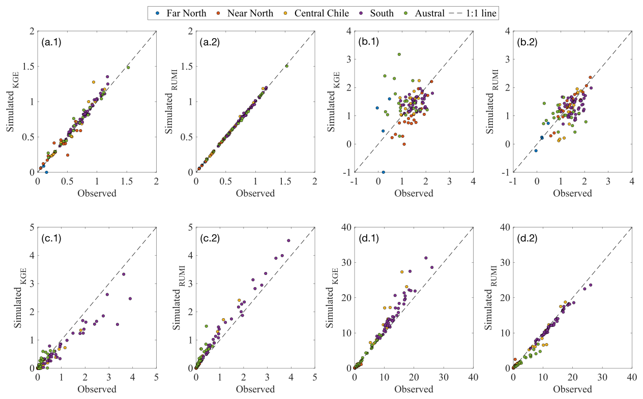
Figure 6 Observed and simulated hydrological signatures for each case (a.1, b.1, c.1, d.1: simulated with KGE; a.2, b.2, c.2, d.2: simulated with RUMI). (a) Runoff ratio (TotalRR); (b) streamflow-precipitation elasticity (QP_elasticity); (c) 5th flow percentile of the streamflow (Q5); and (d) 95th flow percentile of the streamflow (Q95). Colours of dots are related to the five considered macroclimatic zones. The dashed line represents perfect agreement between the observed and simulated hydrological signatures. Note that the y-axis limits for the (a.1) plot are truncated for visualisation purposes (original y-axis range: [0, 30]).

4 Strengths and limitations

One of the main strengths of this study was the proposal of a new dimensionless metric to be used as an objective function for rainfall-runoff model calibration. The proposed approach provides a comprehensive measure of the shared information between observed and simulated streamflows, normalises this measure for comparability, and integrates uncertainty quantification in the calibration process. The rescaling of the performance metric ensures intuitive interpretation (RUMI ranges between 0 and 1, the latter being the optimal value), aligning with standard efficiency metrics and making it easy to understand. This study presented a large-sample rainfall-runoff modelling experiment, analysing 99 catchments in a pseudo-natural hydrologic regime that covers five different macroclimatic zones and, therefore, giving robustness to the analysis. The latter ensures a diverse representation of hydrological characteristics and a broad evaluation of the RUMI-based modelling approach. The simplicity of the approach and its capacity to quantify confidence intervals and, therefore, to carry out uncertainty quantification are significant strengths. As demonstrated by the IQR, the median of results, and outliers (see Table 2), simulations during validation are also seen to improve (alongside the calibration results). Also, using the 50 hydrological signatures, the RUMI-based approach was compared by considering different runoff dynamics characteristics, showing improvements for most (82 % of the analysed signatures showed a better correlation with observed data compared to KGE). RUMI-based performances rely on the combination of available information (in terms of observed quantities) and physically based consistency of modelled hydrological processes (BLUECAT alongside entropy-based computations and the deterministic rainfall-runoff model). The RUMI-based modelling implementation is also facilitated by the codes provided in this paper (see “Code and data availability” statement), which enhances the reproducibility of the methodology.

In terms of limitations – and considering that RUMI considers uncertainty quantification in its computing process – we emphasise the fact that other methodologies for such purposes should be tested (such as multi-model ensemble methods or time-varying model parameters; see Gupta and Govindaraju (2023) for a recent review in this regard) – the latter with the intention to quantify the sensibility of RUMI as a function of those additional methodologies. Additionally, RUMI calculations can be computationally intensive. The method's accuracy depends on high-quality input data and the length of the time series (BLUECAT assumes that the calibration dataset is extended enough to upgrade from the deterministic to the stochastic model). It also assumes that observed and simulated streamflows can be effectively described by these measures, which may not capture all dependencies and non-linearities. Finally, entropy and mutual information might be sensitive to outliers.

5 Conclusions

The RUMI-based hydrological modelling approach outperforms KGE-based modelling in both the calibration and validation phases across various performance metrics. This method demonstrates lower variability and a consistent performance improvement. RUMI's capability to quantify uncertainty and incorporate it into the calibration process ensures more reliable predictions. The analysis of hydrological signatures further confirms the superiority of RUMI, with 82 % of the signatures showing a better correlation with observed data compared to KGE. RUMI offers a valuable tool for hydrological modelling, enhancing the understanding and prediction of streamflow under different hydrological conditions. Even though the data used followed quality control, there are still some potential issues in terms of time discretisation or input variable interpolation. Additionally, some catchments in northern Chile have low annual precipitation and, therefore, a high aridity index. In such catchments, the modelling results were deficient. The latter is probably due to an inconsistency between catchment characteristics, data availability and quality, and model structure.

Possible additional research is as follows: (a) testing the RUMI-based approach with other rainfall-runoff models (lumped, semi-distributed, and distributed hydrological models); (b) testing the RUMI-based approach under other hydro-climatological catchment characteristics and in a higher number of catchments; (c) testing alternative uncertainty quantification methods; (d) exploring the impact of varying data quality on RUMI performance to establish guidelines for data requirements; (e) testing with higher-resolution data to reduce discretisation issues; and (f) exploring the applicability of RUMI in other disciplines such as meteorology, environmental science, and ecology, where modelling and uncertainty quantification are critical.