the Creative Commons Attribution 4.0 License.
the Creative Commons Attribution 4.0 License.
 | 30 Sep 2025
Can causal discovery lead to a more robust prediction model for runoff signatures?
Hossein Abbasizadeh
Petr Maca
Martin Hanel
Mads Troldborg
Amir AghaKouchak
Runoff signatures characterize a catchment's response and provide insight into the hydrological processes. These signatures are governed by the co-evolution of catchment properties and climate processes, making them useful for understanding and explaining hydrological responses. However, catchment behaviors can vary significantly across different spatial scales, which complicates the identification of key drivers of hydrologic response. This study represents catchments as networks of variables linked by cause-and-effect relationships. We examine whether the direct causes of runoff signatures, representing independent causal mechanisms, can explain these catchment responses across different environments. To achieve this goal, we train the models using the causal parents of the runoff signatures and investigate whether it results in more robust, parsimonious, and physically interpretable predictions compared to models that do not use causal information. We compare predictive models that incorporate causal information derived from the relationships between the catchment, climate, and runoff characteristics. The Peter and Clark (PC) causal discovery algorithm is applied separately for 11 runoff signatures to derive causal relationships between catchment attributes, climate indices, and corresponding runoff signatures. Three prediction models – the Bayesian network (BN), generalized additive model (GAM), and random forest (RF) – are used for predictions. The results indicate that among models, BN, a linear model with a structure based on the causal network, exhibits the smallest decline in accuracy between training and test simulations compared to the other models. Across nearly all environments and runoff signatures, using causal parents enhances robustness and parsimony while maintaining the accuracy of GAMs. While RF achieves the highest overall performance, it also demonstrates the most significant drop in accuracy between the training and test phases. When the sample size for training is small, the accuracy of the causal RF model, which uses causal parents as predictors, is comparable to that of the non-causal RF model, which uses all selected variables as predictors, particularly for low-flow duration, high-flow duration, low flows, and high flows. This study demonstrates the potential of causal inference techniques for interpreting and enhancing the prediction of catchment responses by effectively representing the interconnected processes in hydrological systems in a cause-and-effect manner.
- Article
(7105 KB) - Full-text XML
-
Supplement
(44298 KB) - BibTeX
- EndNote


Hydrological processes result from complex interactions between climate inputs and catchment characteristics (Sivapalan, 2006). These processes manifest in the catchment response at the catchment outlet. Therefore, catchments can be conceptualized as a unit in which the cumulative effect of all interacting processes defines their runoff behavior, commonly referred to as “runoff signatures”. Runoff signatures encapsulate the key characteristics of the runoff process in a catchment, including streamflow magnitude, frequency, and timing. These signatures are essential for a wide range of engineering and scientific applications (Blöschl et al., 2013), especially when causal interpretation or assessment is not possible due to insufficient data. McMillan (2020) outlined a wide range of applications for runoff signatures, such as assessing the performance of hydrological models (Clark et al., 2011; Todorovic et al., 2024), selecting appropriate model structures (Hrachowitz et al., 2014; Spieler and Schuetze, 2024), and estimating parameters (Pokhrel et al., 2012; Pizarro and Jorquera, 2024). They are also instrumental in streamflow prediction in ungauged basins (Yadav et al., 2007; Zhang et al., 2014; Matos and Silva, 2024) and in understanding catchment runoff responses at different spatial and temporal scales (Ficchi et al., 2019).
Although all processes in a catchment contribute to its runoff response, each runoff property (or signature) is directly influenced by a distinct set of climatic and catchment-specific characteristics. As an example, Chagas et al. (2024) studied the regional patterns of low flows across 1400 river gauges in Brazil. These authors showed that catchment characteristics, especially geological properties, have a significantly greater influence on low flows than climate attributes. Guzha et al. (2018) investigated the effects of changes in forest cover on annual mean flow, high flow, and low flow in 37 catchments of different climatic and physiographic properties in East Africa, concluding that not all catchments exhibit a significant response to forest loss. Therefore, it is necessary to identify a set of variables or covariates that is causally associated with a specific runoff signature and can reliably explain it under various environmental conditions. Understanding these variables allows one to explain the signature of interest across environments with different climatic and physiological conditions.
The main drivers of runoff signatures are commonly investigated using classification and regression methods. These techniques are applied to identify the main drivers influencing catchment response and to assess their spatial dependencies. Classification criteria often include runoff properties (Ley et al., 2011; Sawicz et al., 2011; Kuentz et al., 2017), climate, and catchment similarities (Olden et al., 2012; Singh et al., 2016; Yang and Olivera, 2023; Ciulla and Varadharajan, 2024). Additionally, machine learning and statistical methods are widely used for the same purpose. For example, Addor et al. (2018) used RF to predict 15 runoff signatures across 600 catchments in the USA. They showed that climatic attributes are among the most influential predictors of runoff signatures. McMillan et al. (2022) investigated the dominant process by linking climate and catchment attributes to hydrological signatures over large sets of catchments in the USA, the UK, and Brazil. They found that although some signatures, such as runoff ratio and baseflow index, were among the most robust metrics for characterizing processes, in some cases, the correlation found between variables and signatures in a country may not always generalize to others. These authors noted that these diverging correlations could result from statistical associations rather than true causal relationships.
We postulate that investigating the relationship between hydrological variables and cause-and-effect perspectives might solve the problem of diverging correlations reported by McMillan et al. (2022). A variable X is considered the cause of a variable Y if the value of Y depends on or is influenced by X in any given circumstances (Pearl et al., 2016; Pearl, 2009). Therefore, the probability of a target variable, such as a runoff signature, given its causes, should be the same under different conditions or across different environments. Broadly, there are two widely used frameworks for discovering causal relationships and estimating causal effects from observational data, including structural causal modeling (Pearl, 2009) and the potential outcome framework (Rubin, 1974). The methods used to discover causality and to quantify causal effects and their strength are broadly referred to as causal inference methods (CIMs).
One application of CIMs is to complement machine learning approaches by addressing the problems of transfer and generalization (Schölkopf et al., 2021; Ombadi, 2021) by identifying dependencies and confounding factors using multivariate analyses (Runge et al., 2019a). In an under-investigated cause-and-effect relationship, a confounding variable is an unknown or unmeasured variable that influences both the supposed effect and the supposed cause (Pearl et al., 2016). Identifying confounders and unraveling causal effects make CIMs a valuable tool for enhancing the interpretability of Earth system models (Reichstein et al., 2019). CIMs are established based on a robust mathematical framework that identifies conditional dependencies in observational data (Pearl, 2009). This process often involves deriving a causal graph based on our understanding of the conditional dependencies among processes using methods such as the Bayesian network (BN) or Bayesian belief network (Verma and Pearl, 1990).
In the last decade, significant efforts have been made to investigate and develop applications for CIMs in the field of Earth system modeling. These studies, primarily focused on uncovering causal relationships from time series, cover a broad range of topics including climate science (Runge et al., 2019b; Kretschmer et al., 2016), remote sensing (Perez-Suay and Camps-Valls, 2019), soil moisture–precipitation feedback detection (Wang et al., 2018), runoff behavior (Zazo et al., 2020), the causal discovery of summer and winter evapotranspiration drivers (Ombadi et al., 2020), and the study of hydrological connectivity (Sendrowski and Passalacqua, 2017; Rinderera et al., 2018; Delforge et al., 2022). However, the causal relationships between catchment attributes, climate characteristics, and runoff signatures have yet to be thoroughly investigated. A catchment can be represented as a probabilistic network of interconnected processes leading to a runoff signature. To achieve this, catchments can be conceptualized as BNs, where variables are causally linked. BNs, part of the family of probabilistic graphical models, consist of nodes representing variables and directed edges indicating causal directions (Koller and Friedman, 2009). The structure of BNs is usually identified through causal discovery methods and expert knowledge (Runge et al., 2019a). Methods for causal discovery, also known as structural learning or causal search, can be categorized into constraint-based, score-based, and asymmetry-based approaches (Runge et al., 2023). Constraint-based methods use conditional independence tests to identify the causal graph, while score-based methods evaluate multiple causal graphs using a scoring function, selecting the highest-scoring one. Asymmetry-based methods are used to infer causal direction in bivariate relationships (Runge et al., 2023).
One of the most widely used causal discovery algorithms is PC, named after its authors, Peter Spirtes and Clark Glymour (Spirtes et al., 2001). The PC algorithm is a constraint-based method for causal discovery, which means it infers causal relationships by testing for conditional independencies in the data. It operates under the assumption of causal sufficiency; that is, all relevant variables are measured, and there are no unobserved confounders. Given this assumption and a sufficiently large sample size, the algorithm guarantees asymptotically correct results (Glymour et al., 2019). Although this method is used for discovering directed acyclic graphs (DAGs), its results do not fully identify the true causal structure; instead, it outputs a Markov equivalence class, a set of causal graphs that encodes the same conditional independencies. These equivalence classes are typically represented using completed partially directed acyclic graphs (CPDAGs) (Peters et al., 2017). Due to its simplicity, computational efficiency, and strong performance, the PC algorithm has been widely adopted across various fields, such as climate science (Ebert-Uphoff and Deng, 2012; Deng and Ebert-Uphoff, 2014), medicine (Sanchez-Romero et al., 2023), and epidemiology (Petersen et al., 2021).
The information about the causal relationships between catchment variables can be incorporated into prediction models to predict runoff signatures. Predictions using BNs are primarily designed for discrete datasets that can model complex interactions between variables. The rigorous probabilistic theories involved in BNs make them popular for environmental modeling (Aguilera et al., 2011). However, Nojavan et al. (2017) and Qian and Miltner (2015) showed that the results of BNs are influenced by the discretization choice of continuous variables. Inference with BN for continuous variables is still a challenging task (Li and Mahadevan, 2018). Gaussian BN is a widely used method for modeling continuous variables. It assumes that the relationships between variables are linear and that variables follow a Gaussian distribution (Marcot and Penman, 2019). To relax these assumptions, non-parametric continuous BNs have been developed (e.g., Qian and Miltner, 2015). However, Gaussian BNs remain a robust and widely used framework, supported by various software packages (Geiger and Heckerman, 1994). Gaussian BNs have been successfully applied in environmental modeling, particularly for water quality studies, for example, Jackson-Blake et al. (2022) and Deng et al. (2023).
Given the success of Gaussian BNs in other fields, in this study, we adopt Gaussian BNs to predict runoff signatures. The links between variables of BN are derived from the PC causal discovery algorithm. Additionally, two non-linear models – the generalized additive model (GAM) and random forest (RF) – are used in this study. GAM is an extension of the generalized linear model (GLM), which models non-linear relationships between explanatory and response variables using sums of arbitrary functions of the explanatory variables (Hastie et al., 2009). GAMs have been widely used for hydrological studies, including flood frequency analysis (Ouali et al., 2017), low-flow frequency analysis (Ouarda et al., 2018), flood peak prediction (Dubos et al., 2022), analysis of nuisance flooding (Vandenberg-Rodes et al., 2016), spatial analysis of extremes (Love et al., 2020), and climate–crop yield relationships (Zachariah et al., 2021). RFs, first developed by Breiman (2001), are non-linear non-parametric models used extensively for regression, classification, prediction, and variable selection. RF-based models have also been used in the field of environmental modeling, including for flow frequency analysis (Desai and Ouarda, 2021), runoff signature prediction (Addor et al., 2018), water level forecasting (Nguyen et al., 2015), downscaling (Arshad et al., 2024), and understanding drivers of hazards (Seydi et al., 2024).
This study introduces a novel approach for predicting runoff signatures by integrating causal information into predictive models. To the best of our knowledge, causal inference techniques have not yet been applied for this purpose. Unlike previous studies that primarily rely on correlated-based features for predicting a specific catchment response, we take a step beyond mere correlation by focusing on causally relevant variables, specifically causal parents. By integrating causal information into predictive models (GAM and RF), we aim to investigate whether this can enhance the prediction models' robustness, interpretability, and parsimony compared to models that do not utilize causal insights. We assume that a specific characteristic of catchment response is directly influenced by a subset of correlated variables, known as causal parents, rather than by all correlated variables. These causal parents, together with the runoff signature, form a causal mechanism that is theoretically independent of other variables and can explain the variations in the signature. In this context, our objective is to test whether this fundamental concept applies to complex real-world hydrological systems. To achieve our objectives, we follow these steps: (1) identify causal relationships between catchment attributes, climate characteristics, and runoff signatures (network structure) using the PC causal discovery algorithm (Spirtes et al., 2001), (2) execute models using both the causal parents (causal models) and all selected variables (non-causal models) for entire catchments and subset of catchments, and (3) evaluate the robustness of the causal and non-causal models.
The Catchment Attributes and MEteorology for Large-sample Studies (CAMELS) dataset is used in this study (Newman et al., 2015; Addor et al., 2017). It includes time series of streamflow and hydrometeorological variables, climatic indices (derived from hydrometeorological time series), catchment attributes, and runoff signatures (derived from streamflow time series) for 671 catchments spanning the contiguous USA. The attributes in the CAMELS dataset are divided into five categories: climate, geology, soil, topography, and vegetation (land cover). CAMELS also includes comprehensive explanations of the techniques employed to derive catchment attributes and a discussion of potential limitations in the data sources. The variables used in this study include catchment characteristics, climate attributes, and runoff signatures, which are outlined in Tables 1 and 2. The streamflow and hydrometeorological time series are not included in this study.
Table 1Catchment and climate attributes used for clustering as well as for causal discovery and prediction of all runoff signatures. Variables shown in bold are those selected for causal discovery and prediction. The variables were calculated over the period from 1 October 1989 to 30 September 2009 (Table 2 in Addor et al., 2018).
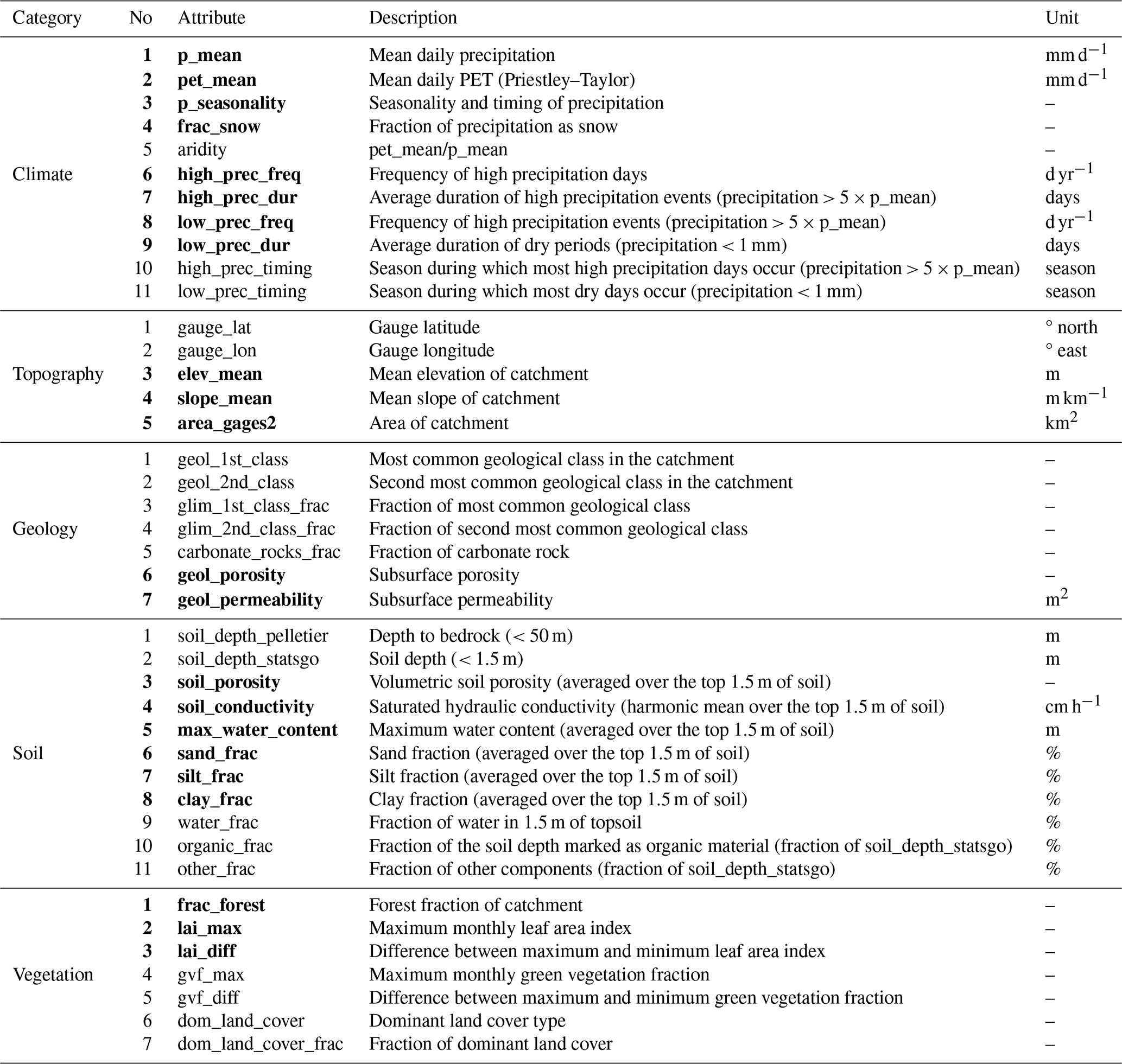
Table 2Runoff signatures (target variables) in the CAMELS dataset, calculated over the period from 1 October 1989 to 30 September 2009.
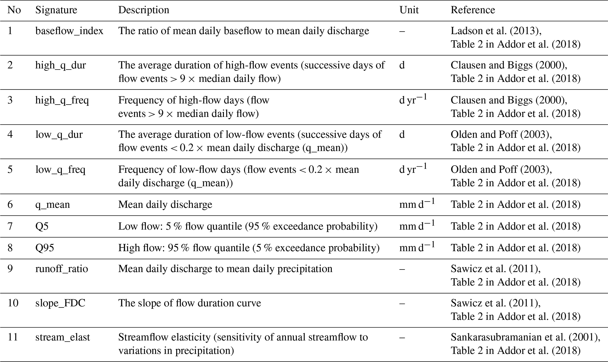
Table 1 includes 41 catchment and climate attributes, including both categorical and continuous variables. In this study, we perform clustering, causal discovery, and prediction, each of which relies on specific assumptions that must be satisfied when applied to our data. Ensuring these assumptions hold is essential for the validity and reliability of the results. All 41 attributes were used in the clustering analysis. However, for the causal discovery and prediction tasks, we used a subset of 22 continuous variables that are most relevant to all runoff signatures. We performed three types of correlation analyses – Pearson, Kendall, and Spearman – to examine the relationships between catchment and climate attributes and runoff signatures. To further assess the predictive power of these attributes, we used the RF algorithm to evaluate feature importance. Variable importance was ranked using the out-of-bag (OOB) approach, based on the mean decrease in accuracy (IncMSE) score. This metric quantifies the increase in prediction error when a variable is excluded from the model, thereby indicating its relative contribution to predicting runoff signatures. The RF algorithm was implemented using the randomForest package in R (Breiman et al., 2024). The results of this analysis are provided in the Supplement.
It is important to note that when constructing a causal graph (directed acyclic graph, or DAG) and performing predictions using BN methods, which are part of the probabilistic graphical model framework, the selected variables (nodes) must not be deterministic functions of one another, as this would violate the conditional independence assumptions underlying the DAG structure (Koller and Friedman, 2009). For this reason, the aridity index, which is the ratio of precipitation to potential evapotranspiration, is excluded from the analysis. The issue of determinism also arises when variables are complementary, such as soil texture components, which are represented as percentages of sand, silt, clay, water, organic matter, and other contents that together sum to 100 %. To ensure valid causal discovery and prediction, we use only a subset of these variables, specifically sand, silt, and clay, in our analysis.
The methodology integrates clustering, causal discovery, and prediction. Figure 1 shows the methodological procedure used in this study. In Fig. 1, causal models refer to the models that use causal parents, and non-causal models use all 22 variables as predictors (the variables shown in bold text in Table 1). Environments are defined as subsets of the dataset obtained through clustering algorithms. Therefore, the word “environment” refers to the clusters or subsets of data. The whole dataset itself is also an environment; however, in this study, we primarily refer to clusters when discussing environments. Baseline models refer to the models that use the whole dataset (i.e., all 671 catchments) for training and testing, and sub-models use subsets of the dataset for this purpose. GAM∼Par and RF∼Par are causal GAM and RF models that employ causal parents for prediction. GAM∼All and RF∼All are non-causal GAM and RF models that use all the selected variables as predictors. A robust model is defined as one that maintains its accuracy across different environments.
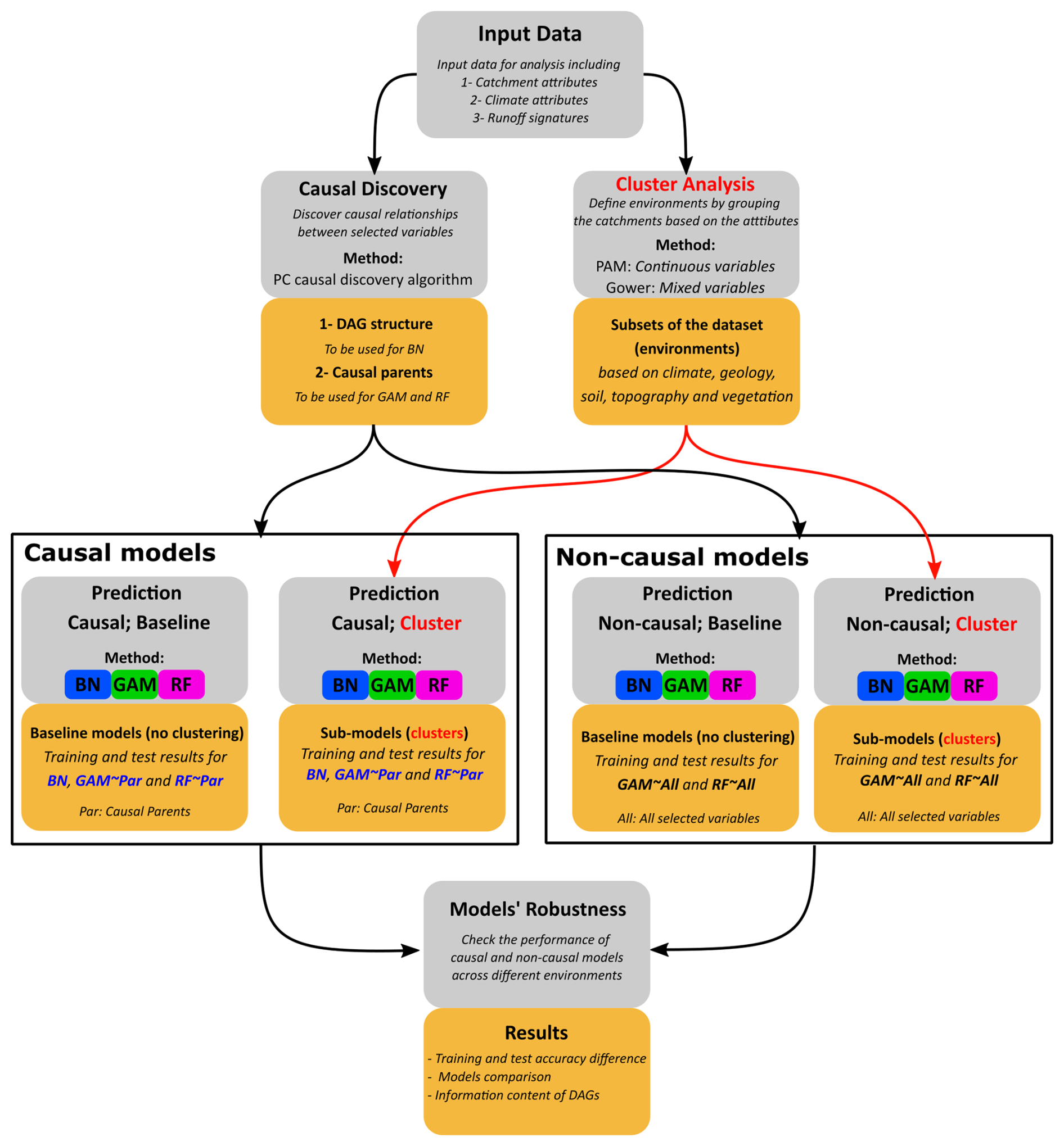
Figure 1Flowchart depicting the steps followed in this study. Gray boxes indicate the procedures, mustard yellow boxes present the results of these procedures, blue text highlights where information about causality is utilized, and the red text and arrows highlight the cluster analysis and indicate where the clustering results are applied. PC refers to Peter and Clark's causal discovery algorithm, PAM stands for partition around the medoids clustering algorithm, and DAGs refers to directed acyclic graphs. BN refers to the Bayesian network, GAM refers to the generalized additive model, and RF refers to random forest. GAM∼Par and RF∼Par are causal models (GAM and RF) using only causal parent variables for prediction, while GAM∼All and RF∼All are non-causal models that use all selected variables as predictors. Baseline models refer to models that use the entire dataset (all 671 catchments) for training and testing, while sub-models use only subsets of the dataset or clusters.
In this study, we explore the concept of independent mechanisms in the context of modeling runoff signatures. The independent mechanism assumption suggests that the causal generative process of a system's variables is made up of self-contained modules that operate independently, without influencing or providing information to one another, and these mechanisms stay stable even when the data distribution changes (Schölkopf et al., 2012; Peters et al., 2017). Using the directed acyclic graph (DAG) obtained from causal discovery, we identified the causal parents of the target runoff signature, which represent the independent causal mechanism generating this variable. Independent mechanisms, as modular components, can be trained separately across different environments and tend to be more adaptable and reusable, a quality we refer to as robustness in this study (Parascandolo et al., 2018). They may also be easier to interpret and provide more insight since these causal mechanisms correspond to physical mechanisms. To evaluate the real-world applicability of this mechanism, we used the identified causal parents as predictors to train RF and GAM. This approach tests whether the independent mechanism derived from the DAG can effectively explain and predict the target variable, supporting the idea that these causal conditions serve as robust and interpretable modules in the prediction of runoff signatures.
To achieve this, we use the whole dataset for the prediction in baseline models and subsets of the dataset in sub-models, both with and without utilizing causal information, corresponding to causal and non-causal models, respectively. If the causal models perform comparably to or better than non-causal models across different environments, it indicates that causal parents are adequate in explaining the target variable. In this situation, we can also conclude that the causal discovery is able to recover the direct causes of the runoff signature. In cases where causal models outperform non-causal ones, it suggests that some covariates in the non-causal models may represent spurious correlations, negatively impacting performance in that specific environment. Furthermore, the robustness of the models is assessed by comparing their accuracy in training and test settings and checking whether the difference between causal and non-causal models is statistically significant in both settings. The methods used to calculate statistical significance tests comparing causal and non-causal models are presented in the Supplement.
The steps are explained in the following sections.
3.1 Clustering
The CAMELS dataset provides five categories of catchment and climate attributes for each catchment (Table 1). Clustering catchments based on each category of attributes is assumed to provide groups of catchments with homogeneous characteristics (Blöschl et al., 2013). Clustering is used to group the CAMELS catchments into different categories based on specific attributes. Any given catchment will belong to one climate attribute cluster, one soil attribute cluster, one topographic attribute cluster, one geological cluster, and one vegetation cluster (i.e., each catchment is “assigned” five cluster values – one for each attribute). The whole process of training and testing the models is now (also) done on separate attribute clusters only, so basically, it is only done on a subset of the available data but using data that share certain characteristics. The causal parents and selected variables are, however, the same whether we use clustering or not.
We investigate the performance of the sub-models within each cluster of catchments. Each cluster is considered a new environment with certain properties that are used to investigate the robustness of models with and without causal parents. The selected covariates remain the same across all environments for each runoff signature. Within each cluster or environment, covariate properties are assumed to be homogeneous with respect to specific attributes, allowing us to train and test models using variables with consistent properties. Defining environments as subsets of data is inspired by Peters et al. (2016). Here, we use a clustering analysis to define these subsets, resulting in environments with specific properties. Therefore, clusters can be considered as subsets of data where the distribution of covariates shifts from one cluster to another. This variation across clusters provides a framework for exploring the underlying independent causal mechanisms of each runoff signature.
The causal independent mechanism (the target variable and its parents) for each signature remains unchanged if there is a change in the distribution of parents (Woodward, 2008). Therefore, causal models (models with causal parents as explanatory variables) are expected to perform with consistent accuracy across different environments. This concept is influenced by the covariate shift assumption (Quionero-Candela et al., 2009). Covariate shift states that if variable Y is to be predicted from a set of variables X, and X is the cause of Y, the properties of conditional probability P(Y|X) remains unchanged across all environments if the distribution of X changes. This information will help to investigate the performance of the causal compared to the non-causal models.
Two clustering methods are employed to group the catchment attributes in the CAMELS dataset. The K-medoids or partitioning around medoids (PAM) clustering algorithm (Kaufman and Rousseeuw, 1990) is used for categories of attributes with continuous variables, namely soil and topography. PAM is a more robust method for handling outliers and noise than the K-means method. The Gower distance (Gower, 1971) is used for mixed variables. This method is developed for datasets containing continuous, binary, or multi-attribute variables (Hennig and Liao, 2013). The elbow and silhouette methods are used to find the optimum number of clusters.
3.2 Causal discovery
Causal discovery is used to partially or fully infer the causal structure from observational data or distribution under certain assumptions (Heinze-Deml et al., 2018a). Here, we try to find causal structures from the observational data without specifying the underlying physical equations using a causal discovery method. Causal discovery is applied to each runoff signature along with 22 variables from the CAMELS dataset in order to identify the causal graph associated with each runoff signature.
3.2.1 PC causal discovery algorithm
In this study, the constraint-based PC causal discovery algorithm (Spirtes et al., 2001), named after its authors, Peter Spirtes and Clark Glymour, is used. The PC algorithm recovers the causal graph from observed data by testing which variables are conditionally independent of each other. These independencies are seen as constraints to satisfy the true data-generating process. The PC algorithm outputs a completed partially directed acyclic graph (CPDAG), which represents a Markov equivalence class of causal structures. This means that instead of identifying a single unique directed acyclic graph (DAG) that fully describes the causal relationships among variables, the PC algorithm returns a set of DAGs that are indistinguishable based on observed statistical dependencies alone. These DAGs all share the same conditional independence; that is, the probability distribution of the variables satisfies the Markov property with respect to each of them. The CPDAG captures this equivalence class by showing which edges are directed and which are only known to exist but not in which direction (undirected edges).
To recover a valid CPDAG using the PC algorithm, certain assumptions must be satisfied to ensure the causal structure is identifiable from the data. These include the causal Markov condition, which links the graph structure to statistical independencies; the faithfulness condition, which ensures that all observed independencies are due to the graph structure or that the distribution is faithful to DAG (Peters et al., 2017); and causal sufficiency, which assumes there are no unmeasured confounders.
To construct the causal graph, PC begins with the assumption that every variable is potentially connected to every other variable, forming a fully connected undirected graph. Then, the algorithm starts removing edges between variables based on statistical tests of conditional independence. The key idea is that if two variables are conditionally independent given some set of other variables, then there is no direct causal link between them, so the edge connecting them can be removed. By checking different sets of conditioning variables and removing the edges accordingly, the PC algorithm recovers the underlying skeleton of the graph; that is, the undirected structure that shows which variables might have a direct relationship.
Once the skeleton is established, the PC algorithm proceeds to orient the edges using specific rules based on the results of the conditional independence tests. A key orientation rule involves identifying v-structures or unshielded colliders. If variables A and B are both connected to a third variable C (i.e., A–C–B), variables A and B are not connected to each other, and variable C was not in the conditioning set that rendered A and B independent, then the structure is oriented as a collider (A → C ← B). After identifying all the v-structures, the PC algorithm applies a set of logical rules to orient the edges throughout the graph while avoiding cycles and introducing new v-structures. However, some edges remain undirected when the available conditional independence information is insufficient to determine a unique orientation without introducing ambiguity or inconsistency with the test results. These undirected edges represent causal relationships whose direction cannot be resolved from the data alone without further assumptions (Meek, 1995; Spirtes et al., 2001).
The results of the PC causal discovery algorithm depend on the alpha value (also called the significance level or threshold). The alpha value is used during conditional independence tests to decide if an edge should be removed. If the p value of a test exceeds the alpha threshold, the algorithm considers the variables to be conditionally independent and removes the edge. Therefore, the value of alpha directly affects the sparsity and structure of the resulting causal graph. The variation in alpha value affects the skeleton and orientation of the graph produced by the PC algorithm (Kalisch et al., 2012). Furthermore, the sample size affects the results of PC, as the algorithm relies on statistical tests of conditional independence to determine the graph structure. As the sample size increases, the accuracy of these tests improves, making it more likely for the algorithm to recover the correct causal structure, or more precisely, the correct Markov equivalence class. Identifying the correct structure of a BN, which relies on independence testing similar to that derived from the PC algorithm, requires substantially more data than approximating the underlying distribution. Underfitting, where true edges are missed, is especially likely when sample sizes are small, as shown in Zuk et al. (2012). Thus, considering these issues, we aim to address the choice of alpha values and sample sizes in the following sections.
3.2.2 Background knowledge and edge assumptions
Background knowledge can significantly enhance causal discovery by reducing ambiguity in the orientation of edges and narrowing the space of plausible causal graphs. According to Perković et al. (2017), incorporating background knowledge, such as known edge directions or variable orderings, into a CPDAG results in a CPDAG that they refer to as a maximally oriented partially directed acyclic graph (maximal PDAG). A maximal PDAG often contains fewer undirected edges and thus represents a smaller Markov equivalence class. This improves the identifiability of causal relationships and allows for a more accurate estimation of causal effects. Similarly, Bang and Didelez (2025) demonstrate that tiered background knowledge, derived from temporal or hierarchical structures, can be encoded as forbidden edge directions to guide constraint-based algorithms. Their algorithms show that such knowledge not only improves the clarity but also reduces the number of independence tests and possible equivalence classes, enhancing both computational efficiency and discovery accuracy. To obtain a maximal PDAG and avoid implausible edge orientations, we define some edge assumptions by excluding the implausible edges before running the PC algorithm. The edge assumptions are as follows:
-
Climate variables cannot cause topography variables.
-
Soil variables cannot cause climate variables.
-
Geological variables cannot cause climate variables.
-
Climate variables cannot cause geological variables.
-
Vegetation variables cannot cause climate variables, except for potential evapotranspiration.
-
Vegetation variables cannot cause topographic variables.
-
Vegetation variables cannot cause geological variables.
-
Soil variables cannot cause topographic variables.
-
Runoff signatures cannot have child nodes.
It is important to note that many of these causally implausible links, such as climate-influencing topography, may become plausible when considered over geological timescales. The final assumption, which treats the runoff signature (the target variable) as a sink node by preventing it from causing other variables, implies that its causal parents correspond to its Markov and stable blankets. The Markov blanket of a node consists of its parents, its children, and the parents of its children. Conditioning on the Markov blanket of a node makes the node independent of the rest of the DAG (Pearl, 1988). This setting also makes the target variable’s causal parents equivalent to its stable blanket for regression. This is because the causal parents form a subset of the Markov blanket, and interventions on non-parent nodes do not affect the functional relationships underlying the causal mechanism of the target variable (Pfister et al., 2021).
3.2.3 Implementation and evaluation of the PC algorithm's results
The PC algorithm assumes that the variables are normally distributed. Therefore, the Box–Cox transformation is applied to the data (Dutta and Maity, 2020). Since the results of the PC algorithm can depend on the order of the input variables, we use the PC-stable variant (Colombo and Maathuis, 2014), which addresses this issue by ensuring order-invariant outputs. The bnlearn R package (Scutari, 2010) is used to apply the PC algorithm. Mutual information with the James–Stein estimator (Hausser and Strimmer, 2009) is chosen as the conditional independence test.
In this study, we run the PC algorithm for 22 variables along with a runoff signature. We do this for 11 runoff signatures. The sample size for each variable is roughly 670 data points. Since the result of the PC algorithm is sensitive to the sample size and significance threshold (alpha value), we set the significance threshold to 0.2 to allow for a more inclusive initial edge selection. The high significance level helps to reduce the risk of a type I error, that is, missing true causal edges. However, it increases the risk of type II errors, which is the appearance of false-positive edges. The edge assumptions, defined as a denial list, help to prevent the occurrence of a large number of false-positive edges. We evaluate the resulting CPDAG following the approach proposed by Petersen et al. (2021). First, we assess the stability of the discovered edges by performing 1000 bootstrap resamples (Scutari and Nagarajan, 2013) of the data and applying the PC algorithm to each resample, using a stricter significance threshold of 0.05 for conditional independence tests. We then measure the strength of each edge based on its frequency across the bootstrap iterations. The resulting edge strength estimates, which represent the proportion of bootstrap samples in which each edge appears, are then mapped onto the initial CPDAG obtained from the PC algorithm. This approach enabled us to evaluate the stability and sparsity level of the causal links if we had a dataset with a larger sample size. Then, we use regression modeling with cubic splines as a heuristic test for conditional independence, assessing the statistical significance of each edge present in the CPDAG produced by the PC algorithm. We fit cubic spline regression models for each pair of variables (Xi,Xj), using the conditioning set Z = . We regress Xi once on Z and once on {Xj}∪Z (forward direction). To account for potential asymmetry in the relationships, we repeat the same procedure by regressing Xj on Z and on {Xi}∪Z (backward direction). In total, we fit four models for each pair of adjacent variables in the CPDAG, which are as follows:
where g and are identity functions and s and are cubic splines. The likelihood ratio tests are applied to compare M0a and M1a as well as M0b and M1b to estimate the conditional independence between pairs of adjacent nodes. We consider variables (Xi,Xj) adjacent if at least one of the following null hypotheses is rejected:
Since no distributional assumptions are made, this test establishes a necessary, but not sufficient, condition for conditional independence between variables (Petersen et al., 2021). Here, we report the p values obtained from the likelihood ratio test for each edge in the DAGs, without assuming a specific alpha threshold. The alpha value can be set to 0.05 to be compared with the significance threshold used in bootstrapping DAGs or to a value between 0.05 and 0.2 to be compared with the edges identified in the initial PC algorithm run. The p value provides insight into the trade-off between statistical significance and edge strength.
The DAG for each runoff signature is derived from the corresponding CPDAG by orienting the undirected edges. This is done in a way that avoids introducing new unshielded colliders, structures in which two parent nodes point to a common child without being connected to each other. Introducing such colliders would change the set of conditional independencies encoded by the original CPDAG.
3.3 Prediction models
The obtained DAG structures are used to predict runoff signatures using Bayesian network (BN) methods. Additionally, generalized additive models (GAMs) and random forests (RFs) are applied to predict runoff signatures: once using all variables in the DAGs (non-causal models) and once using only the causal parents of the target nodes (causal models).
3.3.1 Bayesian network (BN)
Having the graph structure from the causal discovery algorithm, the data are fitted to the graph, and the parameters are estimated. Gaussian BN is used for inference purposes. Gaussian BN belongs to the family of continuous BNs, meaning the nodes are continuous variables. The conditional dependencies are linear and follow the joint Gaussian distribution. The prediction is made using the averaging likelihood simulation with 500 random sampling numbers. The averaging likelihood simulation is a particle-based approximate method for inference in probabilistic graphical models. This method calculates the weight of samples according to the likelihood of evidence, which is a specific value of the signature of interest. It adds up these weights for each sample (Koller and Friedman, 2009). Since Gaussian BN is limited to capturing only linear relationships, other non-linear prediction methods are also employed in this study, which are explained in the following sections.
3.3.2 Generalized additive model (GAM)
The generalized additive model (GAM) (Hastie et al., 2009) is also chosen to handle non-linear relationships between predictors and runoff signatures. GAMs are extensions of generalized linear models (GLMs), which can identify the linear and non-linear relationship between response and explanatory variables. This method uses scatterplot smoothers (e.g., smoothing spline or kernel smoother) to fit the additive functions. In this study, the penalized regression spline is used as the smoother. This smoother prevents the model from overfitting, where the coefficients of the penalized spline decrease (Dubos et al., 2022). The calculation is done using the mgcv R package (Wood, 2018). We used cubic regression splines for the smooth terms. The outcome variable is continuous, and we used the default identity link function with a Gaussian error distribution. The GAMs were fitted using restricted maximum likelihood to estimate the smoothing parameters. The model predicts the signatures once with all variables derived from the feature selection (non-causal model) and once with only the causal parents of the signatures derived from the causal discovery section (causal model).
3.3.3 Random forest (RF)
The last prediction model used in this study is RF. This method estimates response variables using multiple regression trees. Besides its ability to identify non-linear patterns in the data, the likelihood of overfitting in RF is low because the model's prediction is an ensemble of multiple predictions. Therefore, it can deliver an accurate prediction with little computational effort. These features in the RF model help to identify the issues of linearity and overfitting in the BN and GAM models, respectively. The randomForest R package (Breiman et al., 2024) is used, with the number of trees set to 500 to stabilize the prediction (Addor et al., 2018). Similar to GAM, RF is run twice: once using all the selected variables as the predictors of the runoff signature (non-causal model) and once using only the causal parents as predictors (causal model).
For all models – BN, GAM, and RF – the environments are divided into training and test sets, where 75 % of the catchments are randomly selected for training, and the remaining 25 % are used for testing. This process is repeated 500 times using bootstrapping to generate different combinations of training and test sets. This approach provides a range of model performances, and their average performance is used for comparison. Importantly, the training and testing of models are conducted within the same environment, meaning that models trained for a specific environment are tested within that same environment. For example, if a model is trained on catchments from a specific climate category cluster, it is also tested on catchments within that same cluster. The models are executed for the whole dataset (baseline models) and each cluster of categories (sub-models). The models' accuracy is evaluated using root mean squared error (RMSE) and R-squared metrics between predictions and observations. The iteration provides 500 RMSE and R-squared for each run, and the accuracy is reported as their mean value. The following section discusses the obtained results of this study.
4.1 Clustering results for each category
The clustering classifies the catchments according to the five categories. Time series data are not used for clustering analysis, and only catchment attributes available in the CAMELS dataset, as listed in Table 1, are utilized for this purpose. Table 3 shows the methods used for clustering, the optimum number of clusters according to the elbow and silhouette scores, and the number of catchments in each cluster. Figure 2 illustrates each cluster's spatial extent of catchments along with two chosen variables. The obtained results from the cluster analysis for each category of attributes are as follows:
-
Climate attributes. Climate attributes in the CAMELS dataset are derived from the area-weighted averaging of meteorological forcing time series from 1 October 1989 to 30 September 2009. The cluster analysis shows four distinct climate categories, which spread in the east (cluster 1), the midwest (cluster 2), the west (cluster 3), and the northwest (cluster 4) (Fig. 2a). The largest group of catchments belongs to cluster number 1, with 334 members in the north and southeast of the USA (Table 3). This cluster receives an average of 3.5 mm daily precipitation and has 2.8 mm daily evapotranspiration. Other clusters have the following average precipitation and evapotranspiration levels: cluster 2 has 2.3 mm of precipitation and 2.7 mm of evapotranspiration, cluster 3 has 5.5 mm of precipitation and 2.4 mm of evapotranspiration, and cluster 4 has 2.0 mm of precipitation and 3.3 mm of evapotranspiration.
-
Soil attributes. The soil property data, derived from the State Soil Geographic Database (STATSGO), provides information about the top 2.5 m of soil. However, the CAMELS dataset only includes soil data for the top 1.5 m. Soil texture is represented in 16 classes, of which there are 12 classes based on the United States Department of Agriculture (USDA) and four non-soil classes. The saturated hydraulic conductivity and soil porosity are calculated based on the sand and clay fractions using a multiple regression analysis. A cluster analysis identifies six groups of catchments. There is no distinctive spatial pattern among the soil clusters. However, clusters 2 and 3 are mostly spread across the east and west coastlines (Fig. 2b). The maximum water content and porosity values are influenced by soil texture, which defines the proportion of sand, clay, silt, and other materials. For example, cluster 6 shows the highest soil porosity and maximum water content (Fig. 2b). This cluster has the highest percentage of clay (26 %) and silt (47 %) fractions among all clusters.
-
Topographic attributes. The topographic information of catchments, namely catchments' contours, is determined using geospatial fabric (Viger and Bock, 2014) and Geospatial Attributes of Gages for Evaluating Streamflow (GAGES II) methods (Falcone, 2011). These methods are used to determine the area, and the digital elevation model (DEM) is clipped for each catchment. This category is divided into four distinctive clusters. Cluster 1 contains catchments located in the northeast, which are catchments with a low elevation and slope (Fig. 2c). Cluster 2 consists of catchments along the west coast, spread from the west to the northwest. The catchments with the lowest elevation and slope are in cluster 3, located in the southeast. Cluster 4 contains the highest elevation catchments in the Rocky Mountains (Fig. 2c).
-
Geological attributes. The geological variables in the CAMELS datasets are derived from the Global Lithological Map (GLiM) (Hartmann and Moosdorf, 2012) and the Global HYdrogeology MaPS (GLHYMAPS) (Gleeson et al., 2014). From the GLiM dataset, 16 lithological classes are identified, and their proportional areas are calculated for each catchment. The GLHYMAPS dataset is used to estimate subsurface permeability and porosity (Addor et al., 2017). This category is divided into seven groups. Unlike the climate and topography categories, this category does not show a distinguishable spatial pattern (Fig. 2d). However, the catchments with the highest geological porosity are mainly concentrated in the southeast, and those with the lowest are located in the west (Fig. 2d).
-
Vegetation attributes. Vegetation is represented using two indicators: vertical density, measured by the leaf area index (LAI), and horizontal density, measured by the green vegetation fraction (GVF). These measurements are derived from a 1 km resolution product of the Moderate Resolution Imaging Spectroradiometer (MODIS). The vegetation or land cover category is divided into six different groups (Fig. 2e). The spatial pattern of the vegetation is influenced by the climate and topographic categories. According to Fig. 2e, the catchments with the highest forest fractions have the highest maximum LAI and are located in the northeast and east of the study area. This area has high precipitation and low evapotranspiration (Fig. 2a). The lowest vegetation cover belongs to the central and southern parts of the USA, which are in clusters 4 and 6.
Table 3Attribute categories, clustering methods, number of clusters, and catchments per cluster.
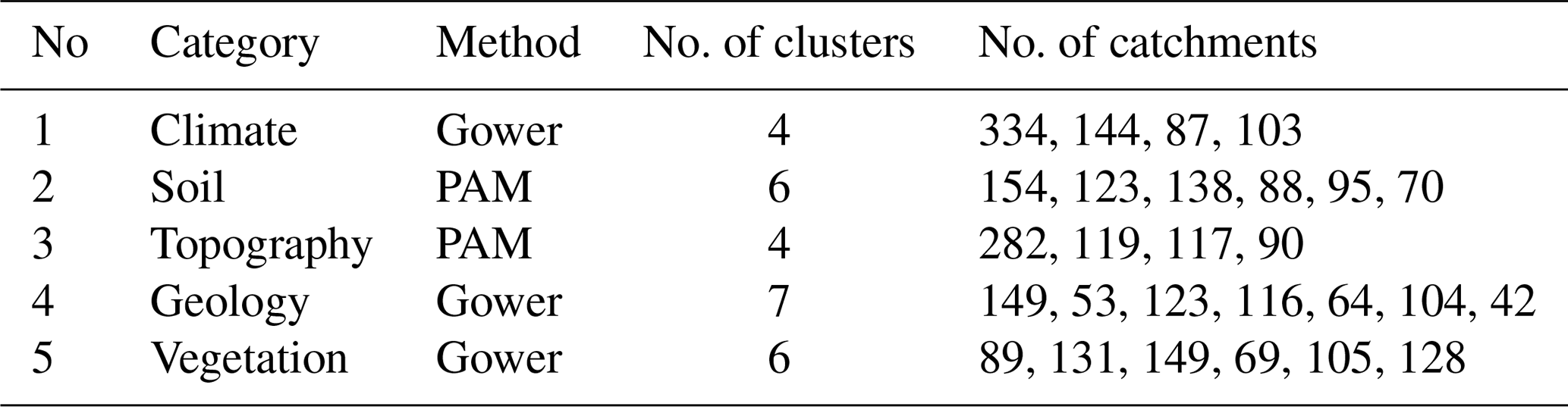
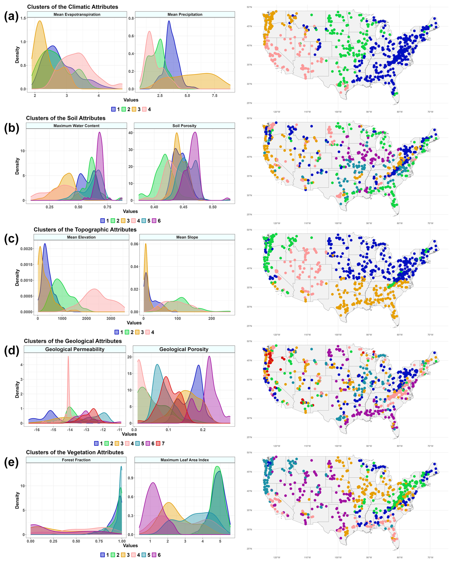
Figure 2The spatial pattern of clusters (right column) and the density of two variables of its corresponding category (left column). The plots show spatial patterns of (a) climate attributes, (b) soil attributes, (c) topographic attributes, (d) geological attributes, and (e) vegetation or land cover attributes.
These clusters are subsets of the CAMELS dataset, with specific properties and different numbers of catchments to be used for runoff signature prediction. They help to evaluate the models' performance in different environments, analyze the effect of causal parents as predictors, and assess how the number of data points impacts the training and test simulations.
4.2 Identification of causal links
The PC algorithm results identify the causal links between all variables. The output of the PC algorithm is a completed partially directed acyclic graph (CPDAG), which may contain undirected edges. In all CPDAGs obtained in this study, the connection between mean elevation and mean slope remains undirected. To derive a fully directed acyclic graph (DAG) from the CPDAG, we orient this edge from mean elevation to mean slope. As shown in Fig. 3b, this orientation does not introduce any unshielded colliders or cycles in the graph. Therefore, we ensure that the resulting DAG belongs to the same Markov equivalence class as the CPDAG produced by the PC algorithm.
Figure 3a shows the obtained DAG for the baseflow index. The signature (red node) has four direct causes or parents (yellow nodes). Figure 3c shows the nodes that form the independent causal mechanism for the baseflow index, shown by the green line. The identified causal parents of the baseflow index include variables related to catchment storage, such as groundwater and snow storage, which are physically meaningful. For each recovered edge, we report both the edge strength and the p value from the likelihood ratio test, as shown in Fig. 3a. The causal models, ∼Par, are trained in the causal mechanism to predict the baseflow index (Fig. 3b). The causal parents in the independent mechanisms also form the Markov and stable blankets for the baseflow index. The structure and variables of the DAG remain unchanged across all environments; only the values of the variables change across environments. DAGs can show the order in which the variables are connected. For instance, the climate and vegetation variables in Fig. 3a are controlled by topographic attributes, which are gauge latitude, mean elevation, and mean slope. These variables are independent of other categories in the DAG since they do not have any parents belonging to the other categories. Furthermore, the causal parents of the signatures, which are identified by the PC algorithm, are not necessarily the most influential variables derived from the correlation and variable importance analysis (see Sect. S1 in the Supplement).
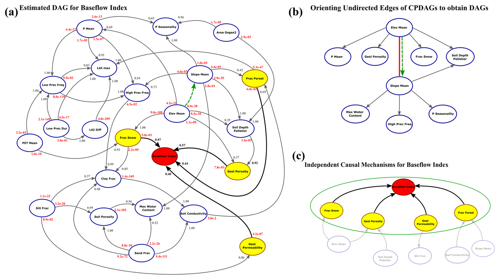
Figure 3(a) Directed acyclic graph (DAG) for the baseflow index. Arrows indicate the causal links between variables. The dashed green arrow represents an oriented edge that was originally undirected in the CPDAG, derived from the PC algorithm. The red node denotes the target variable (runoff signature), and the yellow nodes represent its causal parents. The red numbers at the beginning of each arrow correspond to the p values from the likelihood ratio tests, and the gray (or black for the target variable) numbers indicate the edge strengths derived from 1000 bootstrap resamples. The node variables are explained in Table 1. (b) The part of the CPDAG that contains an undirected edge. Orienting this edge does not introduce any new unshielded colliders. (c) The independent causal mechanism for the baseflow index, which is represented by the red and yellow nodes.
Table 4 shows the causal parents, the p value of the likelihood ratio test, and the edge strength for each runoff signature. The number of parents varies from 2 to 5 variables. We compared the performance of the models using only parents (causal models) to the models using all the selected variables as explanatory variables (non-causal models). The models are executed for the 671 catchments as baseline models and for each cluster as sub-models. The results reveal the models' behaviors in different environments (clusters) compared to the baseline models.
Table 4Causal parents of the runoff signatures derived from the PC algorithm. P values are obtained from the likelihood ratio test, and the edge strengths are derived from the frequency of edges that appear in 1000 bootstrap resamples.
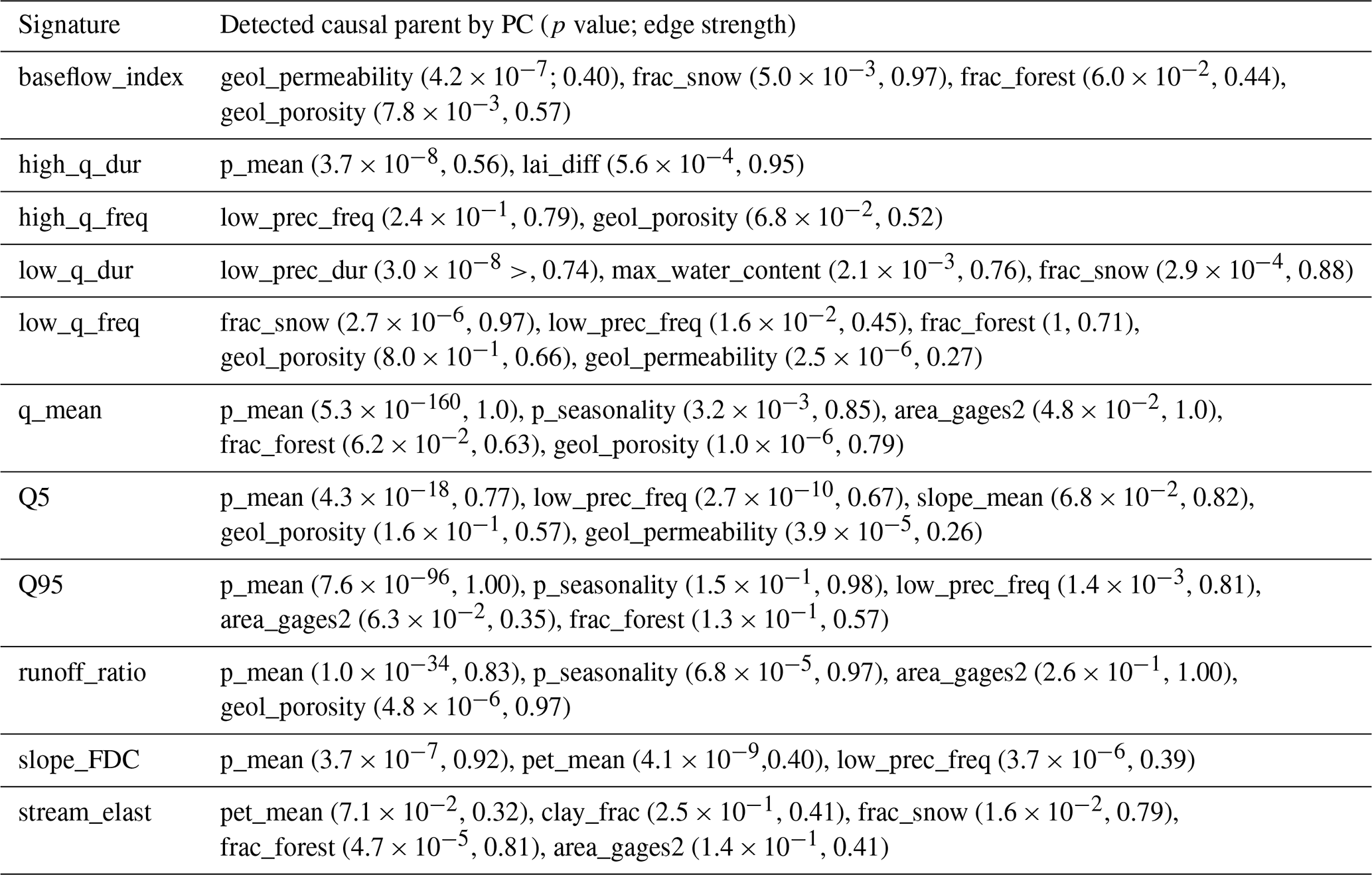
The obtained DAGs, presented in the Supplement, reveal consistent causal relationships between catchment and climate attributes across all runoff signatures, although the strength and significance of the edges vary. In all cases, topographic variables directly influence climate, vegetation, soil, and geological attributes. Climate variables influence vegetation and all runoff signatures (Table 4). Only two edges connect climate and soil variables specifically, from high precipitation frequency and the fraction of snow to the clay fraction. Across all DAGs, these edges consistently exhibit high strength and statistical significance. Soil variables influence vegetation, specifically the fraction of forest, as well as geological variables. However, these variables act as causal parents for only two runoff signatures, namely low-flow duration and streamflow elasticity. Vegetation attributes do not drive other catchment attributes. They are influenced by climate, topography, and soil variables. However, they directly affect six runoff signatures, including baseflow index, high-flow duration, low-flow frequency, mean flow, high flow, and streamflow elasticity (Table 4). The geological variables are influenced by topography and soil. They are among the causal parents of baseflow index, high-flow frequency, low-flow frequency, mean flow, low flow, and runoff ratio (Table 4). The edges in the obtained DAGs are generally characterized by high strength and statistical significance. However, the link between low precipitation frequency and maximum leaf area index stands out as the weakest, with a strength of less than 1 % and a marginal significance level (p value slightly below 0.1). Notably, this link is absent in the DAGs corresponding to high-flow duration, high-flow frequency, low-flow frequency, and the slope of the flow duration curve.
4.3 Performance of the baseline models (prediction using the whole dataset)
The models' performance is evaluated according to the value of RMSE, R-squared between observation and prediction, and the differences between the training and test results. The obtained results for each signature are shown in Fig. 4, Table A1, and Fig. 5. The results are derived from the simulation using the whole dataset (671 catchments), which we call the baseline. Baseline models are considered the most accurate models, in which 75 % of the whole dataset is used for training and 25 % for test simulation. The training and test sets are randomly sampled 500 times, and models are executed after each sampling. The gray dots in Fig. 4 indicate the simulation results for each model's execution. The simulation for GAM and RF models is done twice, once using all the predictors, which are shown by GAM∼All and RF∼All (non-causal models), and once using only causal parents as predictors, GAM∼Par and RF∼Par (causal models).
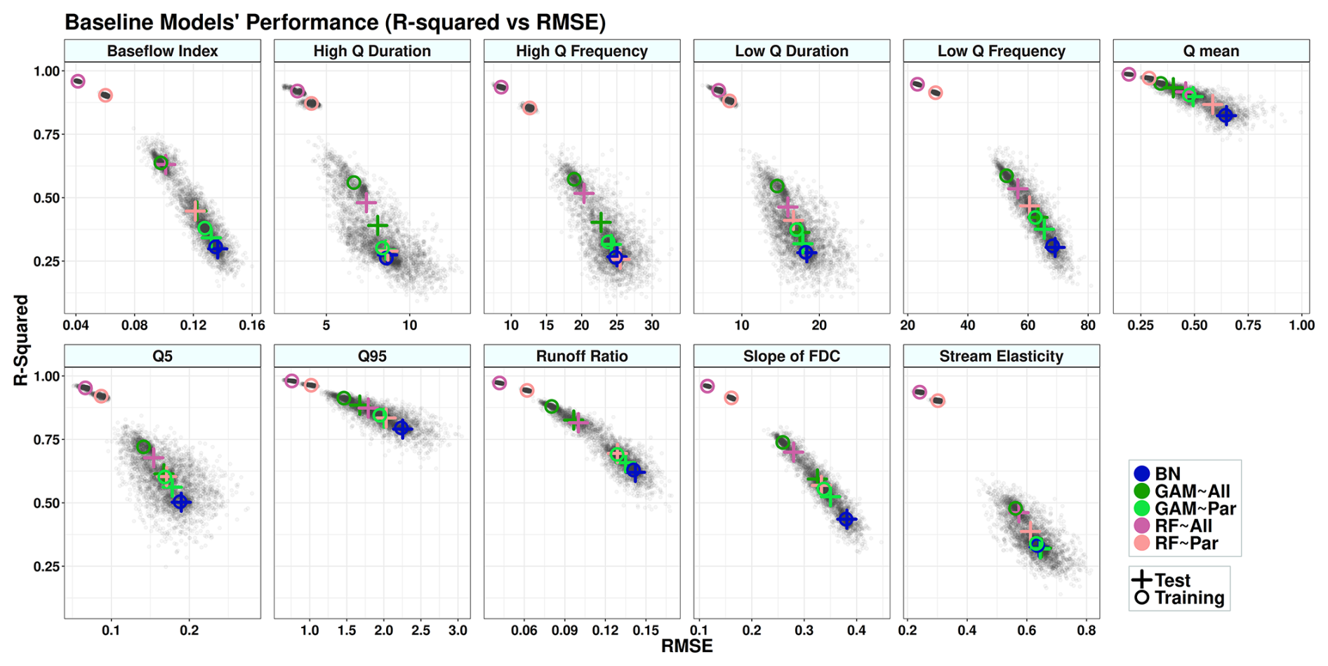
Figure 4Performance of the models: R-squared vs. RMSE. Each colored circle and cross represent the centroid of a set of 500 data points (gray dots) generated from the models' execution. Circles indicate the training results, and crosses indicate the test results. In the legend, “All” refers to using all variables as predictors (non-causal model), and “Par” refers to using only parent variables as predictors (causal model). BN refers to the Bayesian network, GAM refers to the generalized additive model, and RF refers to random forest.
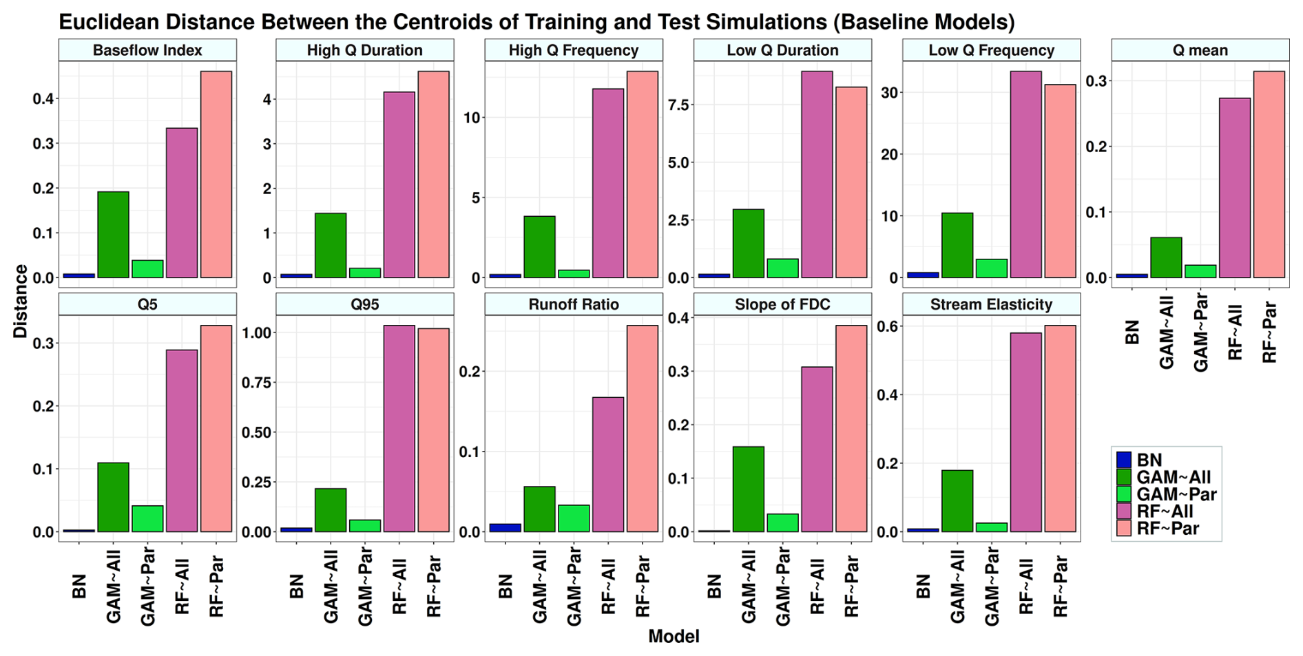
Figure 5The Euclidean distance between the centroid points of training and test simulations in Fig. 4. In the legend, “All” refers to using all variables as predictors, and “Par” refers to using only parent variables as predictors. BN refers to the Bayesian network, GAM refers to the generalized additive model, and RF refers to random forest.
Figure 4 and Table A1 show that reducing the number of predictors decreases the models' accuracy. Among all models, RF models are the most accurate despite showing the most significant drop in accuracy between training and testing simulations (Fig. 5). The R-squared values from the non-causal RF model (RF∼All), in which all selected variables are used as predictors, are compatible with the results obtained from the study of Addor et al. (2018). Using causal parents for RF simulations (RF∼Par) leads to a greater distance between training and test results compared to using RF∼All for some signatures. These signatures are baseflow index, runoff ratio, and the slope of the flow duration curve with 38 %, 53 %, and 25 % increases in distance, respectively, caused by using the causal model (Fig. 5). The causal model slightly reduces the gap between training and test results for low-flow duration, low-flow frequency, and high-flow magnitude, with improvements of 7 %, 6 %, and 1 %, respectively. Similar to the RF model, the accuracy of GAMs is decreased by reducing the number of predictors from all selected variables to parent variables (Table 4 and Fig. 5). However, unlike RF, the distance between the training and test accuracy in R-squared versus RMSE space significantly decreases by using the causal model for GAM (Fig. 5). This distance decreases from 41 % for the slope of flow duration curve to 87 % for the high-flow frequency (Fig. 5). Finally, BN is the least accurate model in capturing the variance since it is a linear model; however, it shows almost the same R-squared and RMSE values in training and testing simulations. As seen in Fig. 5, BN has the shortest distance between training and testing compared to the other two models.
We see that when the training set is large, the accuracy of the non-causal models is higher (GAM∼All and RF∼All). However, this pattern might not be the same if the size of the training set is reduced. Testing the models in different environments with different properties and sizes can help us to understand how these models perform. In this study, environments are clusters of catchments, defined according to each category of attributes (Table 3) that result in homogeneous hydrological properties. The selected variables for the DAG structure and analysis are assumed to be the same, both with and without clusters. However, in the analysis based on clusters, the model's parameterization and predictions are derived from a smaller subset of data compared to the baseline models. The direct causes of signatures are assumed to be the same across all clusters. Therefore, causal models are assumed to result in robust prediction in different environments. This idea is investigated in the following sections.
4.4 The performance of models across different clusters (sub-models)
The results of this simulation indicate different models' behaviors across clusters, which are shown in Fig. 7, Tables 5, A1, A2, and A3, and Sects. S2 and S3. According to the results, GAM∼All shows high accuracy during training across most clusters but performs poorly during testing. The distance between training and testing for GAM∼Par is lower than for GAM∼All in all clusters. This may be due to overfitting in GAM∼All when the sample size is small, resulting in its performance being statistically insignificant from, or in most cases lower than, GAM∼Par across all environments in the test mode. On the other hand, RF∼All shows the highest performance in most cases in both training and testing modes. However, in many cases, RF∼Par performs comparably to RF∼All, despite using significantly fewer predictors. In the case of the BN model, which is linear, it generally exhibits the lowest accuracy compared to GAM and RF. However, it also shows the smallest drop in accuracy between training and testing simulations (see Sect. S2 and Tables S1 and S2). The simulation results for each runoff signature are discussed in the following sections.
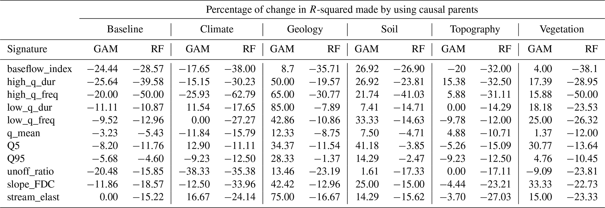
Table 5Comparison of R-squared values between causal and non-causal models presented as percentages. Negative values indicate a decrease in R-squared when using causal models compared to non-causal models. The R-squared values for each category are calculated using the weighted mean, with weights based on the proportion of catchments in each cluster relative to the total number of catchments. The values of R-squared can be found in Tables A2 and A3.
4.4.1 Baseflow index
The four parents of this signature belong to the climate, vegetation, and geology categories (Table 4). The identified causal parents exhibit both high statistical significance and strong edge strength (Table 4 and Fig. S23). The models in the climate, topography, and some clusters of soil groups perform well compared to the baseline (Fig. 6). Although RF∼All demonstrates the best performance, in most cases, the difference between the accuracy of RF∼All and RF∼Par in the test set is negligible, for example, in the soil category clusters 3, 4, and 5, or geology clusters 2 and 7 (Fig. 6 and Table S2). BN has the shortest distance between training and testing (Fig. 7). The decrease in R-squared made by GAM∼Par is improved through a −24 % drop for the baseline model to +9 % for geology, +27 % for soil, and +4 % for the vegetation categories in the sub-models (Table 5). For the climate and topography categories, the accuracy drop caused by using GAM∼Par is 6 % and 4 % smaller in the sub-models compared to the baseline model. The use of causal RF (RF∼Pa) results in a 25 % drop in accuracy in the baseline model. This reduction becomes more pronounced in the sub-models, except for the soil category, where the accuracy drop is 2 % smaller than in the baseline.
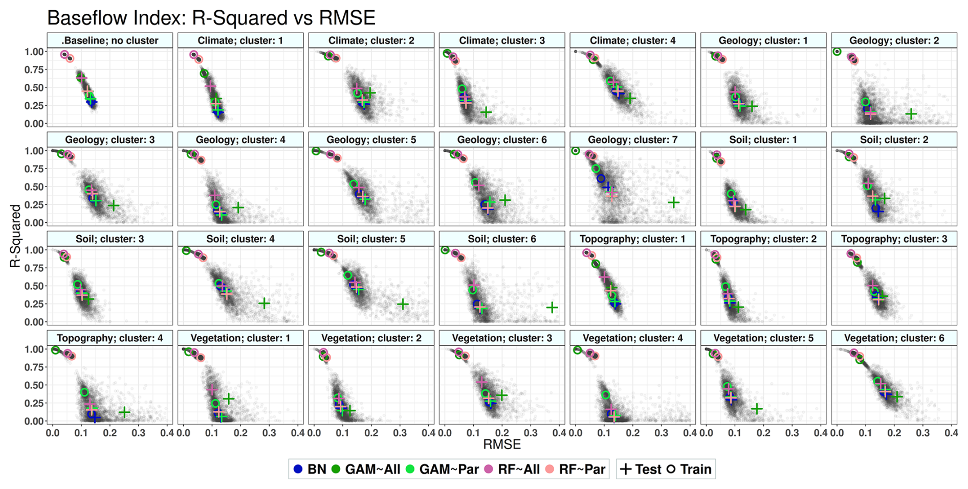
Figure 6Performance of the models for baseflow index: R-squared vs. RMSE. Each colored circle and cross represent the centroid of 500 data points (gray dots) generated from the models' execution. Circles indicate the training results, and crosses indicate the test results. In the legend, “All” refers to using all variables as predictors (non-causal model), and “Par” refers to using only parent variables as predictors (causal model). BN refers to the Bayesian network, GAM refers to the generalized additive model, and RF refers to random forest. The results for other signatures are provided in the Supplement.
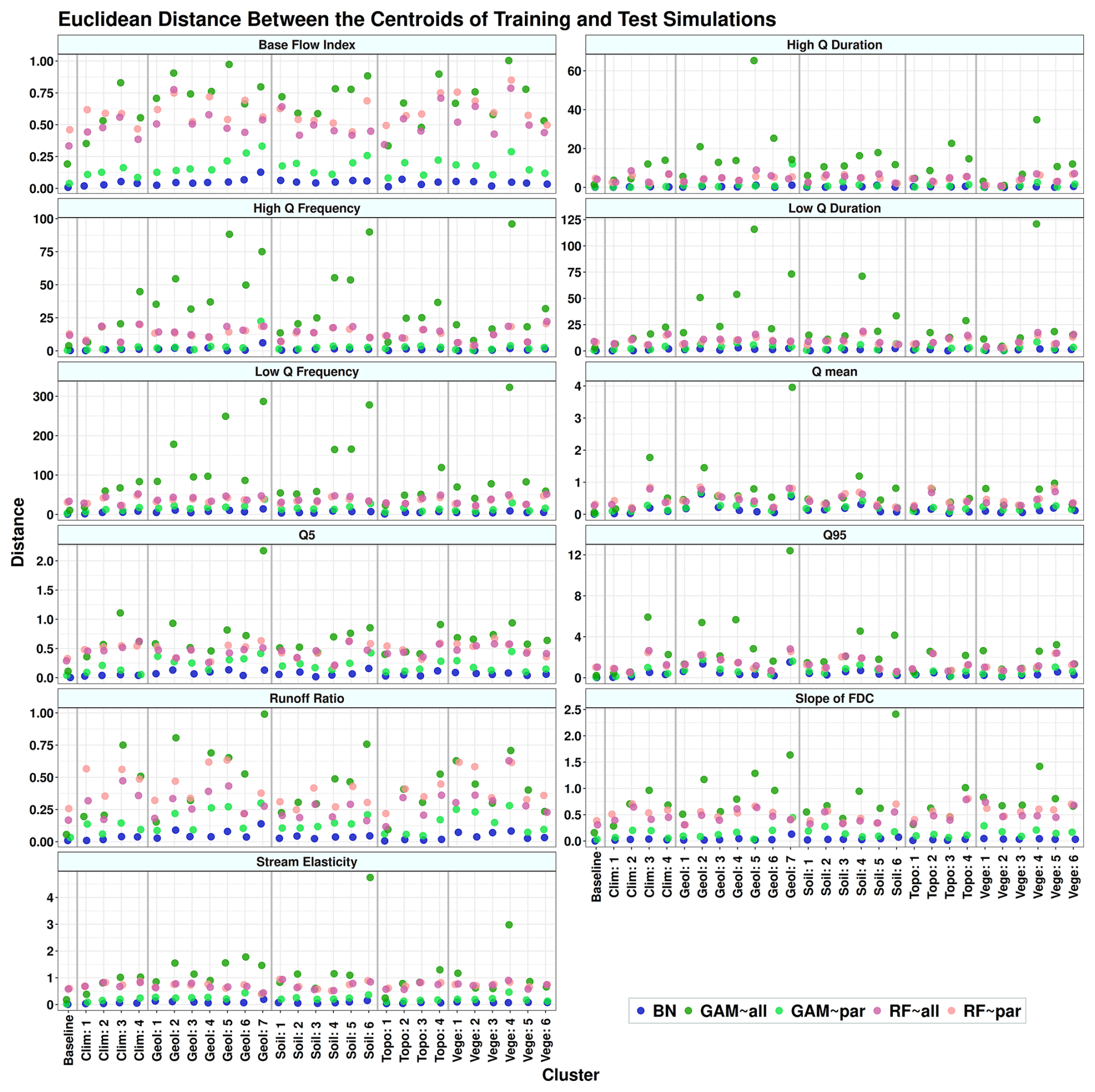
Figure 7The Euclidean distance between the training and test simulations for runoff signatures across different environments for each sub-model. In the legend, “All” refers to using all variables as predictors (non-causal model), and “Par” refers to using only parent variables as predictors (causal model). BN refers to the Bayesian network, GAM refers to the generalized additive model, and RF refers to random forest. On the x axis, Baseline means simulation without any clustering and is done for all 671 catchments. Clim stands for climate, Geol for geology, Topo for topography, and Vege for vegetation. The numbers in front of these names on the x axis represent the clusters' numbers.
4.4.2 High-flow duration
This signature has two causal parents belonging to the climate and vegetation categories (Table 4). The two causal parents of the high-flow duration exhibit both high statistical significance and strong edge strength (Table 4 and Fig. S25). The models perform well across some clusters of the soil and geology categories compared to the baseline (Fig. S26). GAM∼All shows very high accuracy in the training sets, in some cases higher than RF, and a significant drop in accuracy in the test sets (Fig. S26). In addition, the distance between training and the test is higher than GAM∼Par in all cases (Fig. 7). The causal GAMs show robust performance for all environments (Table S1). The distance between training and test simulations in RF∼Par is mainly smaller than RF∼All (Fig. 7). In many cases, the difference between causal and non-causal RF models is negligible (Table S2 and Fig. S26). Although BN shows less accuracy compared to GAM and RF, it outperforms these models in some soil and geology clusters. In addition, in geology cluster 5, BN and GAM∼Par perform better than RF∼All. The accuracy difference between causal and non-causal sub-models is significantly smaller than that of baseline models (Table 5). The use of causal parents as predictors leads to a 26 % and 40 % drop in R-squared in the GAM and RF simulations, respectively. Although the causal models use only two predictors compared to 22 in the non-causal models, the inclusion of causal parents increases the accuracy of GAM by up to 50 % in the geology, soil, topography, and vegetation categories. Additionally, they help to reduce the accuracy drop of RF in the sub-models relative to the baseline model.
4.4.3 High-flow frequency
This signature has two parents belonging to the climate and geology categories (Table 4). Unlike high-flow duration, the causal parents of the high-flow frequency does not show high statistical significance, with a p value of 0.24 and 0.06 for low precipitation frequency and geological porosity, respectively; however, they show acceptable edge strength, with 79 % for the former and 52 % for the latter (Table 4 and Fig. S27). Models perform well across some clusters of the climate, soil, and geology categories. However, there is no single category within which all models outperform the others (Fig. S28). For instance, the models perform well in vegetation cluster 5 (Fig. S28), which are catchments with a high percentage of vegetation cover (Fig. 2). In general, GAM∼All does not show acceptable performance in the test set, and its accuracy in many cases is lower than linear BN (Fig. S28). However, GAM∼Par demonstrates a better performance by reducing the distance between training and test simulations (Fig. 7) and increasing accuracy compared to GAM∼All across all clusters (Fig. S28 and Table S1). Similarly, RF∼Par decreases the distance between the training and testing across most of the clusters, although for the baseline models, this distance is smaller for RF∼All than for RF∼Par (Fig. 7). However, the difference between RF∼All and RF∼Par is negligible in only three environments, namely geology 5 and 7 and soil 5. For the rest of the environments, RF∼All is more accurate (Table S2). In most cases, the accuracy of GAM∼Par is higher than RF∼Par. Using causal parents leads to a decrease in R-squared in the baseline model for both GAM and RF by −20 % and −50%, respectively. While this behavior remains for RF across sub-models, the causal parents increase the accuracy of GAM by up to 65 % (Table 5).
4.4.4 Low-flow duration
This signature has three parents belonging to the climate and soil categories (Table 4). All causal parents of the low-flow duration exhibit both high statistical significance and strong edge strength (Table 4 and Fig. S29). Training and test simulations performed well across all topographic clusters except for cluster number 4, where catchments have high elevations (Figs. 2 and S30). The signature also shows high predictability in clusters with high precipitation intensity (climate cluster 3) and clusters with low soil porosity (soil cluster 2) or clusters with low maximum water content (soil cluster 3). GAM∼Par performs better in different clusters than GAM∼All by reducing the distance between training and test simulations and increasing the model's accuracy (Table S1). This distance is almost the same across clusters for RF∼Par and RF∼All and, in some cases, smaller for RF∼Par. In most environments, the difference between RF∼Par and RF∼All is not significant (Table S2). Using causal parents results in a decrease in the R-squared values of approximately 10 % for both GAM and RF. However, causal parents improve the accuracy of GAM across all categories by up to 85 %, whereas for RF the pattern is reversed, with accuracies dropping by up to 15 %.
4.4.5 Low-flow frequency
This signature has five parents: two belonging to climate, one to vegetation, and two to geological categories (Table 4). Three out of the five causal parents of low-flow frequency exhibit both high statistical significance and strong edge strength. However, despite the relatively high edge strengths – 71 % for forest fraction and 66 % for geological porosity – the p values from the likelihood ratio test are large (Table 4 and Fig. S31). Models perform well across most clusters of the climate and topography categories (Fig. S30). In most cases, GAM∼All performs poorly compared to GAM∼Par (Table S1). The difference between training and testing is significantly reduced in GAM∼Par. This distance is also reduced in RF∼Par and, in many cases, the performance of BN, GAM∼Par, RF∼Par, and RF∼All are comparable across most clusters (Fig. S32). Causal parents lead to a drop in R-squared of both GAM and RF models. This pattern is the same for RF across the sub-models; however, it leads to improving the accuracy of GAM by up to 33 % (Table 5).
4.4.6 Mean daily runoff
The five parents of the mean daily runoff belong to the climate, topography, vegetation, and geology categories (Table 4 and Fig. S33). All five causal parents of mean daily flow exhibit both high statistical significance and strong edge strength, except for forest fraction, which has a p value of 0.06 in the likelihood ratio test (Table 4 and Fig. S33). This signature is the most predictable runoff signature. All models perform well across all clusters; however, unlike other signatures, the BN and GAM models outperform RF in most cases, for example, geology cluster 2 (Fig. S34). In most cases, the difference between training and test simulations is smaller when using parents, which shows the benefits of using causal parents. In addition, the difference in model accuracy between simulations using only causal parent (∼Par) and those using all variables (∼All) is negligible across almost all clusters, especially for GAM (Table S1). For mean daily flow, the reduction in R-squared resulting from using causal parents as predictors is minimal, even in the baseline models, approximately −8 % for GAM and −5 % for RF. While the accuracy drop in RF increases to as much as −15 %, using causal parents improves GAM accuracy by up to 12 %.
4.4.7 Low flow (Q5)
The five parents of low flow belong to the climate, geology, and topography categories (Table 4 and Fig. S35). Among the causal parents of low flow, which generally exhibit both high statistical significance and strong edge strength, mean slope and geological porosity have higher p values in the likelihood ratio test compared to the other parents, although their edge strengths remain high (Table 4 and Fig. S35). The models' test results are comparable to the baseline models in geology clusters 2 and 4 and soil clusters 2 and 4 (Fig. S36). GAM∼All is outperformed by GAM∼Par and other models in test simulations (Fig. S36 and Table S1). As shown in Fig. S36, models perform well across the topographic category. The difference between training and test simulations is improved in GAM∼Par compared to GAM∼All. This distance for RF∼Par is smaller than for RF∼All across half of the clusters (Fig. 7), and the difference between causal and non-causal RF models is negligible for most environments (Table S2). BN has the smallest difference between training and testing, and its performance is comparable to GAM and RF in most cases. Using parents as predictors increases the accuracy of GAM in the climate, geology, soil, and vegetation categories by 13 %, 34 %, 41 %, and 31 %, respectively (Table 5). For RF, the drop in accuracy remains consistent across baseline and sub-models by around −10 % to −15 % (Table 5).
4.4.8 High flow (Q95)
High flows are among the most identifiable signatures. According to the obtained DAG, high flow is controlled by five causal parents belonging to the vegetation (land cover), climate, and topography categories (Table 4 and Fig. S37). Among all the causal parents of high flow, precipitation seasonality has the highest p value (0.15), despite its strong edge strength (98 %). On the other hand, the catchment area shows the lowest edge strength (35 %) and a relatively high p value (0.06). The rest of the causal parents of this runoff signature exhibit high statistical significance and high edge strength (Table 4 and Fig. S37). The models showed high accuracy across most clusters. Unlike other signatures, the accuracy of RF∼All and RF∼Par models, which are the most accurate overall, is comparable to GAM and BN in certain cases (Fig. S37). The difference between training and test simulations is improved in all clusters when using parents for GAM, except for climate clusters 1 and 2, as well as topography cluster 1 (Table S1). The drop in the models' accuracy, caused by using the causal parents, is smaller compared to the other signatures. R-squared is improved among the geology, soil, and vegetation categories for GAM models (Table 5).
4.4.9 Runoff ratio
Runoff ratio has four parents belonging to the climate, geology, and topography categories (Table 4 and Fig. S39). Although the catchment area has a high p value as a causal parent of stream elasticity, its edge strength is 100 %. All other causal parents of the runoff ratio exhibit both high statistical significance and strong edge strength (Table 4 and Fig. S39). The models perform well across the topographic and soil clusters, and models are more robust across those environments (Fig. S39). Causal models show a negligible difference between training and test simulations for almost all clusters for GAM but not for RF (Fig. 5 and Table S2). The difference between the R-squared values is significantly lower across categories than the baseline models, especially in the geology and soil categories (Table 5).
4.4.10 Slope of flow duration curve
All three parents of the slope of flow duration curve belong to the climate category (Table 4 and Fig. S41). All causal parents of the slope of flow duration curve exhibit both high statistical significance and relatively strong edge strength (Table 4 and Fig. S41). Models in topographic clusters performed well except for cluster 4, where there are catchments with a high elevation and steep slopes. RF∼Par and GAM∼Par perform almost the same across most of the clusters. In most cases, GAM∼Par reduced the difference between training and test simulations compared to GAM∼All (Table S1). The difference between RF∼Par and RF∼All is statistically significant except for two clusters, namely geology cluster 4 and vegetation cluster 1 (Fig. S42 and Table S2). Using causal parents as predictors for the slope of flow duration curve increases the accuracy of the sub-models GAMs by 42 %, 25 %, and 33 % for the geology, soil, and vegetation categories, respectively; however, for the causal RFs, models lead to a decrease in R-squared compared to the non-causal RFs (Table 5).
4.4.11 Stream precipitation elasticity
The five parents of this signature belong to the climate, soil, topography, and vegetation categories (Table 4 and Fig. S43). Among the causal parents, snow fraction and forest fraction exhibit both high statistical significance and relatively strong edge strength. In contrast, the remaining causal parents have either relatively low edge strength or high p values in the likelihood ratio test (Table 4 and Fig. S43). In most cases, the performance of the RF∼All and RF∼Par models in the test mode is comparable (Fig. S44), especially in the geology clusters 2, 3, 5, and 7 (Table S2). The same as with other signatures, GAM∼All performs well only in the training simulation. The difference between causal and non-causal models is not statistically significant for GAMs (Table S1). The distance between training and test simulations in GAM∼Par is smaller than for GAM∼All. This pattern can be seen in only one-third of the clusters for RF models (Fig. 7). According to Table 5, the causal parents lead to an increase in accuracy of GAM of 17 %, 75 %, 14 %, and 15 % for the climate, geology, soil, and vegetation categories, respectively. The performance of RF∼All, RF∼Par, and GAM∼Par are close and comparable in the test simulation (Fig. S43 and Tables 5 and S2).
Figure 8 displays the rankings of the overall performance of models across different environments for all signatures. RF∼All achieved the highest overall accuracy in the baseline mode, where the whole dataset is used. In contrast, BN in the baseline mode ranks 11th, which is the lowest among all models in this mode. This suggests that BN is either not sensitive or only weakly sensitive to sample size. For the other models, the baseline mode consistently ranks among the top 10 in terms of performance. Examining the top 10 rankings of the models across all environments reveals distinct patterns. For BN, the top-performing clusters include two from the climate category, three from geology, two from soil, and one from topography. For GAM∼Par, the top 10 includes the baseline, one cluster each from climate and topography, two from geology and vegetation, and three from the soil category. For GAM∼All, the top ranks comprise the baseline, three clusters from climate, and two clusters each from soil, topography, and vegetation, with none from geology. In the case of RF∼Par, the top 10 includes one cluster each from the baseline, climate, topography, and vegetation, two from geology, and four from the soil category. Lastly, for RF∼All, the top-performing clusters include one from the baseline, one cluster each from geology and topography, two from climate and vegetation, and three from the soil category. Overall, across the top 10 rankings of all models, clusters associated with the soil category appear most frequently, with 15 occurrences. This is followed by the climate category with nine occurrences, geology and vegetation with eight each, and topography with six. Among all environments, climate 4, followed by vegetation 6, are the catchment groups where all models consistently achieve high rankings. Catchments in both climate 4 and vegetation 6 are characterized by relatively low precipitation, high evapotranspiration, and low maximum leaf area index (LAI). On the other hand, vegetation 4, followed by topography 4, are the environments where catchments consistently exhibit the lowest model performance. Catchments in vegetation 4, which are mostly located in the southern and southeastern USA, show high variability in forest fraction and maximum LAI. In contrast, catchments in topography 4 are primarily situated in the Rocky Mountains and are characterized by high elevation and steep slopes.
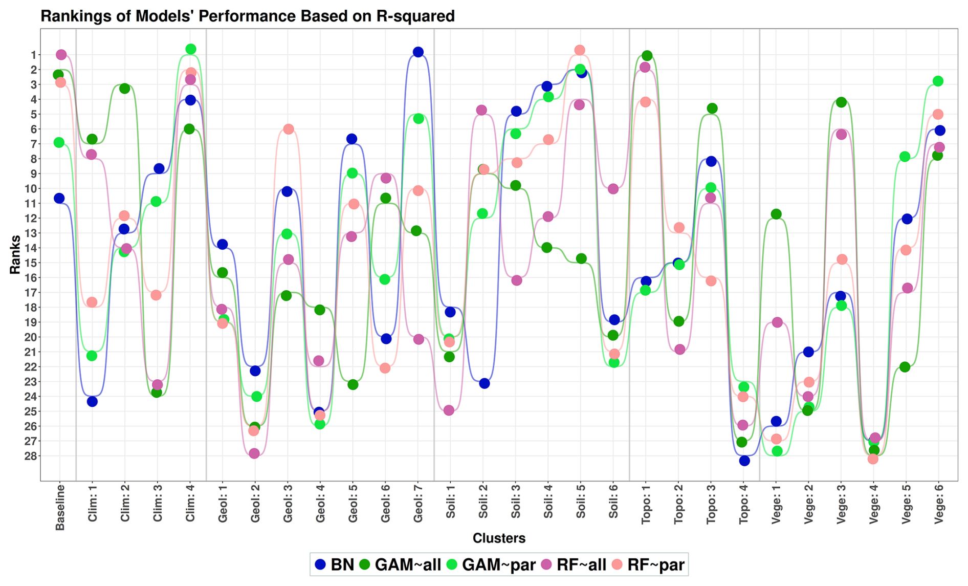
Figure 8Rankings of model performance based on the R-squared values obtained from evaluating their accuracy in predicting all signatures within each cluster. On the x axis, Clim stands for climate, Geol for geology, Topo for topography, and Vege for vegetation.
The aims of this study are to (1) recover the causal graph, represented as a directed acyclic graph (DAG), from catchment attributes, climate characteristics, and runoff signatures; (2) predict runoff signatures using their causal parents as well as all variables in the DAGs; and (3) compare the predictive performance of models using only causal parents (which is an independent causal mechanism) vs. those using all available variables.
A PC-stable algorithm (Colombo and Maathuis, 2014) is used to uncover the underlying causal relationships between runoff signatures, catchment attributes, and climate characteristics. To improve the plausibility of the resulting graph, background knowledge is applied before running PC. Applying background knowledge reduces the risk of spurious or false-positive edges, decreases the number of equivalence classes, and improves the stability of the learned causal graph (Meek, 1995; Spirtes et al., 2001; Perković et al., 2017; Bang and Didelez, 2025). The background knowledge is applied by blocking the implausible edges. In hydrological systems, many causal directions are well understood from process-based reasoning and can be used to restrict the search space of the algorithm. By enforcing these structural constraints (e.g., forbidding reverse causality from runoff to climate), the stability of the learned causal graph is improved, and it allows us to derive a complex causal graph for the catchment area.
To mitigate the rate of false positives and negatives (type I and II errors) in the PC algorithm due to our limited sample size (Li and Wang, 2009), we start the causal discovery analyses by applying a relatively lenient significance threshold (Kalisch and Bühlman, 2007). This threshold increases the risk of false-positive edges. Therefore, to evaluate the quality of the fit, we assess the significance levels of dependencies between adjacent nodes and their corresponding strengths (Petersen et al., 2021). We perform a heuristic evaluation using cubic spline regression and the likelihood ratio test, which allows us to examine non-linear dependencies between adjacent nodes, particularly given that real-world hydrological systems often exhibit non-linear relationships (Kirchner, 2024). To further assess the strength and stability of the inferred links, we perform bootstrap resampling and learn the network structure 1000 times by the PC algorithm using a more stringent significance level (Scutari and Nagarajan, 2013). This approach helps us to investigate potential false-positive edges (type I errors) in the DAG obtained using the lenient significance threshold. Among all the inferred edges in the resulting DAGs, the link between low precipitation frequency and maximum LAI exhibits significantly low strength.
The causal parents identified by the PC algorithm align with the underlying physical processes for most of the signatures. For example, according to the PC results, snow fraction drives the baseflow index, consistent with runoff-generating mechanisms during spring and summer (Gentile et al., 2023). In addition, vegetation and geological variables, which contribute to infiltration and groundwater flow, are causal parents of the baseflow index (Gnann et al., 2019). For high flows (Q95), drivers include precipitation characteristics (mean, seasonality, and frequency), vegetation cover, and catchment area. This suggests that precipitation intensity, often driven by seasonality, influences runoff-generating mechanisms like the infiltration excess process (Nanda et al., 2019). Area and vegetation cover also affect the time concentration and the magnitude of high flows in the catchment area (Sultan et al., 2022). In regions with high mean precipitation and low seasonality, saturation excess runoff mechanisms dominate high flows. Additionally, the PC results for low flows (Q5) include two variables that belong to the geology category, along with two climate variables and one topography variable. Low flows are strongly governed by geological variables in addition to climate and topography (Laaha and Bloeschl, 2006; Giuntoli et al., 2013). However, the causal parents identified by the PC method for the slope of flow duration curve include only climate variables. While this flow signature is strongly influenced by catchment storage, shaped by geology, topography, and land cover (Dey et al., 2024), the method failed to capture these non-climatic influences. The identified causal parents of high-flow frequency include high frequency and geological porosity. However, land cover is also recognized as a key driver of this flow signature (Zabaleta et al., 2018), although it was not captured by the causal discovery method. Therefore, while the PC algorithm identifies physically meaningful causal parents for most signatures, it occasionally fails to capture expected parent variables from certain categories that are known to influence those signatures. Furthermore, the derived causal parents by the PC algorithm are not necessarily the highest correlated variables with the runoff signatures. This highlights the fact that there can be strong causal relationships between variables even when their statistical associations are weak (Gao et al., 2023).
The obtained DAGs indicate that topographic variables drive the climate, vegetation, geological, and soil variables of hydrological systems at the catchment scale. Also, they show that climate attributes influence all runoff signatures, a finding supported by various studies (e.g., Jehn et al., 2020; McMillan et al., 2022). Models perform well across soil and climate clusters for most signatures, with consistently high accuracy rankings (Fig. 8). However, in vegetation cluster 4 and topography cluster 4, all models struggle to predict signatures accurately. In the catchments of vegetation cluster 4, the forest fraction varies almost uniformly between 0 and 1, and, as a result, the maximum LAI exhibits a similar pattern (Fig. 2). This high variability, combined with the small sample size of 69 catchments, leads to poor model performance (Table 3). On the other hand, catchments in topography cluster 4 are characterized by high elevation and low precipitation. The low prediction accuracy in this cluster aligns with Viglione et al. (2013), who observed a decline in prediction model performance in arid catchments. Signatures prove to be more predictable in clusters characterized by high precipitation and low elevation, such as those in climates 1 and 3. This indicates that even in catchments with low precipitation, the transfer of information from precipitation to runoff remains the predominant driver compared to other mechanisms (Neri et al., 2022). According to Fig. 8, models achieve high accuracy scores in regions with high precipitation, such as topography 1 and soil 5. The prediction results indicate that independent variables derived from causal discovery, such as topographic variables, can serve as effective criteria for catchment classification.
The causal GAM, GAM∼Par, outperforms the non-causal GAM∼All in most environments during testing, despite the latter exhibiting higher accuracy in the training mode. GAM∼All achieves its best performance in the baseline mode, where the entire dataset is used for simulation. However, even in these baseline cases, its performance remains comparable to that of GAM∼Par. In the case of RF models, RF∼All achieves the highest accuracy across most environments compared to the other models; however, the performance of RF∼Par is still comparable to RF∼All. The difference in performance between RF∼All and RF∼Par is statistically significant in most cases, as determined by a non-parametric permutation test (see Sect. S3). However, this significance does not merely represent the magnitude of differences between the models. The results of the test also depend on the spread of results across the R-squared and RMSE space. For example, two models might differ in average accuracy, and if their performance varies widely during bootstrapped training and testing, the difference may not be statistically significant. Conversely, even a small difference in accuracy can be statistically significant if the performances of the models are consistently stable. Despite BN having lower accuracy than GAM and RF, it shows the smallest difference between training and test results across all cases. This consistency may be due to the BN structure, which relies on conditional dependencies derived from the causal relationships between variables, although further investigation is needed. The difference between causal and non-causal RF models is mostly statistically significant across clusters of the baseflow index, high-flow frequency, low-flow frequency, mean daily flow, runoff ratio, slope of flow duration curve, and stream precipitation elasticity. For signatures where the difference is insignificant, using causal parents can enhance model parsimony by reducing the number of predictors, improving robustness by maintaining accuracy across environments comparable to non-causal models, and minimizing accuracy reduction between the training and testing phases. This pattern holds for GAM∼Par across most clusters and for RF∼Par across the majority of clusters related to low-flow duration, high-flow duration, low flows, and high flows.
Finally, our results show that causal discovery enhances the representation of physical systems, making models more interpretable and parsimonious, as emphasized by Runge et al. (2019a) and Reichstein et al. (2019). However, there is still room for further investigation, as the causal graphs obtained using the proposed methods require deeper analysis. In this study, we used the PC algorithm to identify the causal parents of runoff signatures. Other methods are specifically designed to target causal parents of a given variable, such as invariant causal prediction (ICP), and could offer additional insights (see Peters et al., 2016; Heinze-Deml et al., 2018b; Kook et al., 2024). The insights gained from causal discovery cannot only improve the understanding of hydrological systems at the catchment scale but also lead to more informed modeling practice (Slater et al., 2024). However, we still need theoretical developments to quantify the stability and robustness of the uncertainty of such a model, particularly when combined with machine learning and classification algorithms (Herman et al., 2015; Singh et al., 2015; AghaKouchak et al., 2022).
This study investigates the application of causal discovery to represent the causal interconnections between variables in hydrological systems. The PC algorithm is used to identify the causal links between catchment attributes, climate indices, and 11 runoff signatures, producing a directed acyclic graph (DAG) for each signature. DAGs reveal the connections between variables, including the direct causes (parents) of the target signatures. Three prediction models – BN, GAM, and RF – in five different settings, namely BN, GAM∼Par, GAM∼All, RF∼Par, and RF∼All, are used to predict runoff signatures. These models are executed on the entire dataset as well as 27 clusters, with each configuration undergoing 500 random samplings of training and test sets, resulting in a total of 140 000 model executions. BN directly utilizes the DAG structure for prediction, while GAM and RF predict the target variable by using both all the variables in the DAG and only the causal parents (the variables that, together with the target variables, form the independent causal mechanism). Each model is run 500 times with random sampling of training and tests for each run. The dataset is then grouped into different clusters based on attribute categories. The clusters serve as new environments to train and test the models, allowing for an assessment of model performance when using causal parents as the explanatory variables. The major outcomes of this research are as follows:
-
The causal parents of the signatures identified by the PC algorithm do not always align with the most influential variables determined by correlation and variable importance analysis. This suggests that strong correlations may result from confounding variables, and causal relationships do not always coincide with high variable importance. This point can impact the robustness of prediction models, especially when the same set of predictor variables is used across diverse environments with varying characteristics.
-
BN shows the smallest decrease in accuracy between the training and test samples, demonstrating high transferability. The accuracy of the models is not sensitive to the training sample size and shift in the distribution of predictors. This indicates that P(Effect ∣ Cause) remains consistent across environments. Although BN’s overall accuracy is lower than that of the non-linear GAM and RF models, it outperforms RF in predicting mean daily runoff and high flows across different environments (clusters).
-
Using causal parents helps to mitigate the overfitting problem and improve the robustness in prediction models, particularly in GAM, when the size of the training set is small.
-
The high accuracy of non-causal models, GAM∼All, in the baseline scenarios may be attributed to overfitting or spurious relationships. This is supported by their reduced accuracy in environments with smaller training sets, highlighting a lack of robustness compared to causal models, which maintain higher reliability under such conditions.
-
Signatures are most predictable when causal and non-causal models are trained on catchments with homogeneous soil properties.
-
Independent variables identified through causal discovery can determine groups of catchments where prediction models exhibit consistent performance. For instance, topographic variables are among the independent variables in this context since all models perform consistently well in clusters 1, 2, and 3, and less effectively in cluster 4. This is also the case for the soil and climate categories, where their variables are mostly independent of the other categories. This information helps to identify environments where training models achieve higher accuracy, reduced uncertainty, and greater robustness.
-
Causal inference methods contribute to improving prediction models' parsimony, interoperability, and robustness in hydrological systems.
In conclusion, causal models maintain acceptable accuracy across environments with varying distributions of explanatory variables (covariates). The DAGs obtained from causal discovery enhance the interpretability of prediction models and offer more informed clustering criteria, which is valuable for regionalization purposes. This study focuses on investigating the direct causes of runoff signatures and their effects on prediction accuracy, but other criteria for selecting predictors from the DAG variables could be explored, for example, investigating the effect of variables with different topological ordering on the target variable, such as root nodes, ancestors of the target variables, etc. In addition, different causal discovery methods may yield alternative DAG structures, which merit further investigation. This work offers insight into the application of causal inference methods in understanding runoff-generating mechanisms in hydrological systems.
While causal inference analysis has been extensively explored in fields such as computer science and medicine, its applications in hydrology are still in their infancy. There is a broad range of potential uses for causal models in hydrology, from identifying the drivers of hydrological anomalies (Tárraga et al., 2024) to linking extreme events with their cascading societal impacts (AghaKouchak et al., 2023). As research in this area progresses, the application of causal inference methods is likely to lead to more accurate and robust predictive models, offering valuable insights into complex hydrological variability.
A1 R-squared and RMSE values for test simulations of baseline models in Fig. 4
Table A1R-squared and RMSE values for test simulations of baseline models. The values are an average of 500 executions of each model.
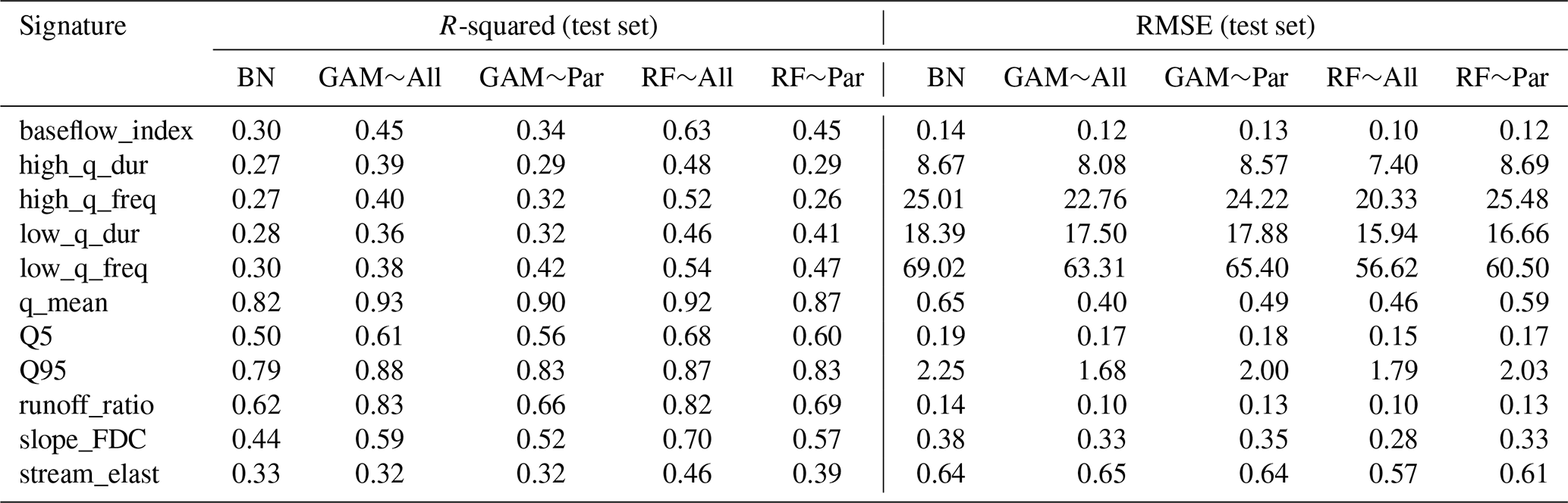
A2 R-squared values used to calculate values in Table 5
Table A2The R-squared values of causal models for each category, which are calculated using the weighted mean. The weights are the ratio of the catchments in each cluster to the total number of catchments.
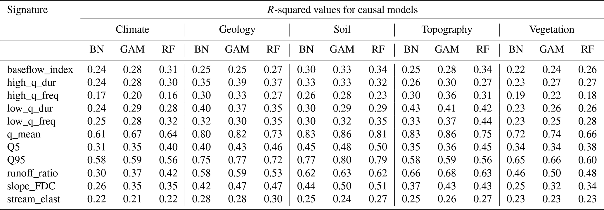
Table A3The R-squared values of non-causal models for each category, which are calculated using the weighted mean. The weights are the ratio of the catchments in each cluster to the total number of catchments.
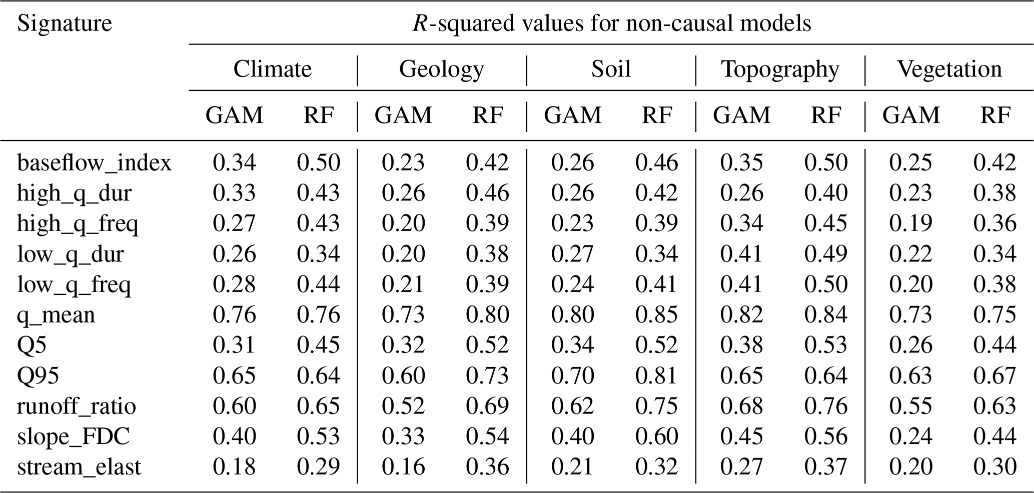
The codes are available on the GitHub repository at https://github.com/abbasizadeh/Catchment-Causal-Discovery (last access: 8 June 2025). The CAMELS attributes are available at https://doi.org/10.5065/D6MW2F4D (Newman et al., 2022).
The supplement related to this article is available online at https://doi.org/10.5194/hess-29-4761-2025-supplement.
HA: conceptualization, methodology, coding and computation, data visualization, writing (review and editing), and funding acquisition. PM: supervision, conceptualization, methodology, writing (review and editing), and funding acquisition. MH: methodology, writing (review and editing), and funding acquisition. MT: conceptualization, methodology, and writing (review and editing). AAK: conceptualization, methodology, and writing (review and editing).
The contact author has declared that none of the authors has any competing interests.
Publisher’s note: Copernicus Publications remains neutral with regard to jurisdictional claims made in the text, published maps, institutional affiliations, or any other geographical representation in this paper. While Copernicus Publications makes every effort to include appropriate place names, the final responsibility lies with the authors.
Computational resources were provided by the e-INFRA CZ project (ID 90254), supported by the Ministry of Education, Youth and Sports of the Czech Republic.
This research has been supported by the Česká Zemědělská Univerzita v Praze (grant nos. 2023B0026 and 2024B0003) and the Ministerstvo Školství, Mládeže a Tělovýchovy (AdAgriF – Advanced methods of greenhouse gases emission reduction and sequestration in agriculture and forest landscape for climate change mitigation (grant no. CZ.02.01.01/00/22_008/0004635)).
This paper was edited by Manuela Irene Brunner and reviewed by three anonymous referees.
Addor, N., Newman, A. J., Mizukami, N., and Clark, M. P.: The CAMELS data set: catchment attributes and meteorology for large-sample studies, Hydrol. Earth Syst. Sci., 21, 5293–5313, https://doi.org/10.5194/hess-21-5293-2017, 2017. a, b
Addor, N., Nearing, G., Prieto, C., Newman, A. J., Le Vine, N., and Clark, M. P.: A Ranking of Hydrological Signatures Based on Their Predictability in Space, Water Resour. Res., 54, 8792–8812, https://doi.org/10.1029/2018WR022606, 2018. a, b, c, d, e, f, g, h, i, j, k, l, m, n, o, p
AghaKouchak, A., Pan, B., Mazdiyasni, O., Sadegh, M., Jiwa, S., Zhang, W., Love, C., Madadgar, S., Papalexiou, S., Davis, S., Hsu, K., and Sorooshian, S.: Status and prospects for drought forecasting: Opportunities in artificial intelligence and hybrid physical–statistical forecasting, Philos. T. Roy. Soc. A, 380, 20210288, https://doi.org/10.1098/rsta.2021.0288, 2022. a
AghaKouchak, A., Huning, L. S., Sadegh, M., Qin, Y., Markonis, Y., Vahedifard, F., Love, C. A., Mishra, A., Mehran, A., Obringer, R., Hjelmstad, A., Pallickara, S., Jiwa, S., Hanel, M., Zhao, Y., Pendergrass, A. G. Arabi, M. Davis, S. J., Ward, P. J., Svoboda, M., Pulwarty, R., and Kreibich, H.: Toward impact-based monitoring of drought and its cascading hazards, Nature Reviews Earth & Environment, 4, 582–595, 2023. a
Aguilera, P. A., Fernandez, A., Fernandez, R., Rumi, R., and Salmeron, A.: Bayesian networks in environmental modelling, Environ. Modell. Softw., 26, 1376–1388, https://doi.org/10.1016/j.envsoft.2011.06.004, 2011. a
Arshad, A., Mirchi, A., Taghvaeian, S., and AghaKouchak, A.: Downscaled-GRACE data reveal anthropogenic and climate-induced water storage decline across the Indus Basin, Water Resour. Res., 60, e2023WR035882, https://doi.org/10.1029/2023WR035882, 2024. a
Bang, C. W. and Didelez, V.: Constraint-based causal discovery with tiered background knowledge and latent variables in single or overlapping datasets, arXiv [preprint], https://doi.org/10.48550/arXiv.2503.21526, 2025. a, b
Blöschl, G., Sivapalan, M., Wagener, T., Viglione, A., and Savenije, H.: Runoff prediction in ungauged basins: synthesis across processes, places and scales, Cambridge University Press, https://doi.org/10.1017/CBO9781139235761, 2013. a, b
Breiman, L.: Random forests, Mach. Learn., 45, 5–32, https://doi.org/10.1023/A:1010950718922, 2001. a
Breiman, L., Cutler, A., Liaw, A., and Wiener, M. randomForest: Breiman and Cutler's Random Forests for Classification and Regression (Version 4.7-1.2), Comprehensive R Archive Network (CRAN), [R package], https://CRAN.R-project.org/package=randomForest, 2024. a, b
Chagas, V. B. P., Chaffe, P. L. B., and Bloeschl, G.: Regional Low Flow Hydrology: Model Development and Evaluation, Water Resour. Res., 60, e2023WR035063, https://doi.org/10.1029/2023WR035063, 2024. a
Ciulla, F. and Varadharajan, C.: A network approach for multiscale catchment classification using traits, Hydrol. Earth Syst. Sci., 28, 1617–1651, https://doi.org/10.5194/hess-28-1617-2024, 2024. a
Clark, M. P., Kavetski, D., and Fenicia, F.: Pursuing the method of multiple working hypotheses for hydrological modeling, Water Resour. Res., 47, W09301, https://doi.org/10.1029/2010WR009827, 2011. a
Clausen, B. and Biggs, B.: Flow variables for ecological studies in temperate streams: groupings based on covariance, J. Hydrol., 237, 184–197, https://doi.org/10.1016/S0022-1694(00)00306-1, 2000. a, b
Colombo, D. and Maathuis, M. H.: Order-Independent Constraint-Based Causal Structure Learning, J. Mach. Learn. Res., 15, 3741–3782, 2014. a, b
Delforge, D., de Viron, O., Vanclooster, M., Van Camp, M., and Watlet, A.: Detecting hydrological connectivity using causal inference from time series: synthetic and real karstic case studies, Hydrol. Earth Syst. Sci., 26, 2181–2199, https://doi.org/10.5194/hess-26-2181-2022, 2022. a
Deng, J., Shan, K., Shi, K., Qian, S. S., Zhang, Y., Qin, B., and Zhu, G.: Nutrient reduction mitigated the expansion of cyanobacterial blooms caused by climate change in Lake Taihu according to Bayesian network models, Water Res., 236, 119946, https://doi.org/10.1016/j.watres.2023.119946, 2023. a
Deng, Y. and Ebert-Uphoff, I.: Weakening of atmospheric information flow in a warming climate in the Community Climate System Model, Geophys. Res. Lett., 41, 193–200, https://doi.org/10.1002/2013GL058646, 2014. a
Desai, S. and Ouarda, T. B. M. J.: Regional hydrological frequency analysis at ungauged sites with random forest regression, J. Hydrol., 594, 125861, https://doi.org/10.1016/j.jhydrol.2020.125861, 2021. a
Dey, P., Mathai, J., Sivapalan, M., and Mujumdar, P. P.: On the regional-scale variability in flow duration curves in Peninsular India, Hydrol. Earth Syst. Sci., 28, 1493–1514, https://doi.org/10.5194/hess-28-1493-2024, 2024. a
Dubos, V., Hani, I., Ouarda, T. B. M. J., and St-Hilaire, A.: Short-term forecasting of spring freshet peak flow with the Generalized Additive model, J. Hydrol., 612, 128089, https://doi.org/10.1016/j.jhydrol.2022.128089, 2022. a, b
Dutta, R. and Maity, R.: Temporal networks-based approach for nonstationary hydroclimatic modeling and its demonstration with streamflow prediction, Water Resour. Res., 56, e2020WR027086, https://doi.org/10.1029/2020WR027086, 2020. a
Ebert-Uphoff, I. and Deng, Y.: Causal Discovery for Climate Research Using Graphical Models, J. Climate, 25, 5648–5665, https://doi.org/10.1175/JCLI-D-11-00387.1, 2012. a
Falcone, J. A.: GAGES-II: Geospatial attributes of gages for evaluating streamflow, Tech. rep., US Geological Survey, https://doi.org/10.3133/70046617, 2011. a
Ficchi, A., Perrin, C., and Andreassian, V.: Hydrological modelling at multiple sub-daily time steps: Model improvement via flux-matching, J. Hydrol., 575, 1308–1327, https://doi.org/10.1016/j.jhydrol.2019.05.084, 2019. a
Gao, B., Yang, J., Chen, Z., Sugihara, G., Li, M., Stein, A., Kwan, M.-P., and Wang, J.: Causal inference from cross-sectional earth system data with geographical convergent cross mapping, Nat. Commun., 14, 5875, https://doi.org/10.1038/s41467-023-41619-6, 2023. a
Geiger, D. and Heckerman, D.: Learning gaussian networks, in: Uncertainty in Artificial Intelligence, Elsevier, 235–243, https://doi.org/10.1016/B978-1-55860-332-5.50035-3, 1994. a
Gentile, A., Canone, D., Ceperley, N., Gisolo, D., Previati, M., Zuecco, G., Schaefli, B., and Ferraris, S.: Towards a conceptualization of the hydrological processes behind changes of young water fraction with elevation: a focus on mountainous alpine catchments, Hydrol. Earth Syst. Sci., 27, 2301–2323, https://doi.org/10.5194/hess-27-2301-2023, 2023. a
Giuntoli, I., Renard, B., Vidal, J. P., and Bard, A.: Low flows in France and their relationship to large-scale climate indices, J. Hydrol., 482, 105–118, https://doi.org/10.1016/j.jhydrol.2012.12.038, 2013. a
Gleeson, T., Moosdorf, N., Hartmann, J., and van Beek, L. P. H.: A glimpse beneath earth's surface: GLobal HYdrogeology MaPS (GLHYMPS) of permeability and porosity, Geophys. Res. Lett., 41, 3891–3898, https://doi.org/10.1002/2014GL059856, 2014. a
Glymour, C., Zhang, K., and Spirtes, P.: Review of Causal Discovery Methods Based on Graphical Models, Frontiers in Genetics, 10, 524, https://doi.org/10.3389/fgene.2019.00524, 2019. a
Gnann, S. J., Woods, R. A., and Howden, N. J. K.: Is There a Baseflow Budyko Curve?, Water Resour. Res., 55, 2838–2855, https://doi.org/10.1029/2018WR024464, 2019. a
Gower, J.: A General Coefficient of Similarity and Some of Its Properties, 27, 857–871, https://doi.org/10.2307/2528823, 1971. a
Guzha, A. C., Rufino, M. C., Okoth, S., Jacobs, S., and Nobrega, R. L. B.: Impacts of land use and land cover change on surface runoff, discharge and low flows: Evidence from East Africa, Journal of Hydrology: Regional Studies, 15, 49–67, https://doi.org/10.1016/j.ejrh.2017.11.005, 2018. a
Hartmann, J. and Moosdorf, N.: The new global lithological map database GLiM: A representation of rock properties at the Earth surface, Geochem. Geophy. Geosy., 13, Q12004, https://doi.org/10.1029/2012GC004370, 2012. a
Hastie, T., Tibshirani, R., Friedman, J. H., and Friedman, J. H.: The elements of statistical learning: data mining, inference, and prediction, Vol. 2, Springer, https://doi.org/10.1007/978-0-387-84858-7, 2009. a, b
Hausser, J. and Strimmer, K.: Entropy inference and the James-Stein estimator, with application to nonlinear gene association networks, J. Mach. Learn. Res., 10, 1469−-1484, 2009. a
Heinze-Deml, C., Maathuis, M. H., and Meinshausen, N.: Causal Structure Learning, Annu. Rev. Stat. Appl., 5, 371–391, https://doi.org/10.1146/annurev-statistics-031017-100630, 2018a. a
Heinze-Deml, C., Peters, J., and Meinshausen, N.: Invariant Causal Prediction for Nonlinear Models, Journal of Causal Inference, 6, 20170016, https://doi.org/10.1515/jci-2017-0016, 2018b. a
Hennig, C. and Liao, T. F.: How to find an appropriate clustering for mixed-type variables with application to socio-economic stratification, J. Roy. Stat. Soc. C-Appl., 62, 309–369, https://doi.org/10.1111/j.1467-9876.2012.01066.x, 2013. a
Herman, J. D., Reed, P. M., Zeff, H. B., and Characklis, G. W.: How should robustness be defined for water systems planning under change?, J. Water Res. Plan. Man., 141, 04015012, https://doi.org/10.1061/(ASCE)WR.1943-5452.0000509, 2015. a
Hrachowitz, M., Fovet, O., Ruiz, L., Euser, T., Gharari, S., Nijzink, R., Freer, J., Savenije, H. H. G., and Gascuel-Odoux, C.: Process consistency in models: The importance of system signatures, expert knowledge, and process complexity, Water Resour. Res., 50, 7445–7469, https://doi.org/10.1002/2014WR015484, 2014. a
Jackson-Blake, L. A., Clayer, F., Haande, S., Sample, J. E., and Moe, S. J.: Seasonal forecasting of lake water quality and algal bloom risk using a continuous Gaussian Bayesian network, Hydrol. Earth Syst. Sci., 26, 3103–3124, https://doi.org/10.5194/hess-26-3103-2022, 2022. a
Jehn, F. U., Bestian, K., Breuer, L., Kraft, P., and Houska, T.: Using hydrological and climatic catchment clusters to explore drivers of catchment behavior, Hydrol. Earth Syst. Sci., 24, 1081–1100, https://doi.org/10.5194/hess-24-1081-2020, 2020. a
Kalisch, M. and Bühlman, P.: Estimating high-dimensional directed acyclic graphs with the PC-algorithm, J. Mach. Learn. Res., 8, 613–636, 2007. a
Kalisch, M., Maechler, M., Colombo, D., Maathuis, M. H., and Buehlmann, P.: Causal Inference Using Graphical Models with the R Package pcalg, J. Stat. Softw., 47, 1–26, 2012. a
Kirchner, J. W.: Characterizing nonlinear, nonstationary, and heterogeneous hydrologic behavior using ensemble rainfall–runoff analysis (ERRA): proof of concept, Hydrol. Earth Syst. Sci., 28, 4427–4454, https://doi.org/10.5194/hess-28-4427-2024, 2024. a
Koller, D. and Friedman, N.: Probabilistic graphical models: principles and techniques, MIT Press, ISBN 9780262013192, 2009. a, b, c
Kook, L., Saengkyongam, S., Lundborg, A. R., Hothorn, T., and Peters, J.: Model-Based Causal Feature Selection for General Response Types, J. Am. Stat. Assoc., 120, 1090–1101, https://doi.org/10.1080/01621459.2024.2395588, 2024. a
Kretschmer, M., Coumou, D., Donges, J. F., and Runge, J.: Using Causal Effect Networks to Analyze Different Arctic Drivers of Midlatitude Winter Circulation, J. Climate, 29, 4069–4081, https://doi.org/10.1175/JCLI-D-15-0654.1, 2016. a
Kuentz, A., Arheimer, B., Hundecha, Y., and Wagener, T.: Understanding hydrologic variability across Europe through catchment classification, Hydrol. Earth Syst. Sci., 21, 2863–2879, https://doi.org/10.5194/hess-21-2863-2017, 2017. a
Laaha, G. and Bloeschl, G.: A comparison of low flow regionalisation methods – catchment grouping, J. Hydrol., 323, 193–214, https://doi.org/10.1016/j.jhydrol.2005.09.001, 2006. a
Ladson, A. R., Brown, R., Neal, B., and Nathan, R.: A standard approach to baseflow separation using the Lyne and Hollick filter, Australasian Journal of Water Resources, 17, 25–34, https://doi.org/10.7158/13241583.2013.11465417, 2013. a
Ley, R., Casper, M. C., Hellebrand, H., and Merz, R.: Catchment classification by runoff behaviour with self-organizing maps (SOM), Hydrol. Earth Syst. Sci., 15, 2947–2962, https://doi.org/10.5194/hess-15-2947-2011, 2011. a
Li, C. and Mahadevan, S.: Efficient approximate inference in Bayesian networks with continuous variables, Reliab. Eng. Syst. Safe., 169, 269–280, https://doi.org/10.1016/j.ress.2017.08.017, 2018. a
Li, J. and Wang, Z. J.: Controlling the False Discovery Rate of the Association/Causality Structure Learned with the PC Algorithm, J. Mach. Learn. Res., 10, 475–514, 2009. a
Love, C. A., Skahill, B. E., England, J. F., Karlovits, G., Duren, A., and AghaKouchak, A.: Integrating Climatic and Physical Information in a Bayesian Hierarchical Model of Extreme Daily Precipitation, Water, 12, 2211, https://doi.org/10.3390/w12082211, 2020. a
Marcot, B. G. and Penman, T. D.: Advances in Bayesian network modelling: Integration of modelling technologies, Environ. Modell. Softw., 111, 386–393, https://doi.org/10.1016/j.envsoft.2018.09.016, 2019. a
Matos, A. C. d. S. and Silva, F. E. O. e: Bayesian estimation of hydrological model parameters in the signature-domain: Aiming for a regional approach, J. Hydrol., 639, 131554, https://doi.org/10.1016/j.jhydrol.2024.131554, 2024. a
McMillan, H.: Linking hydrologic signatures to hydrologic processes: A review, Hydrol. Process., 34, 1393–1409, https://doi.org/10.1002/hyp.13632, 2020. a
McMillan, H. K., Gnann, S. J., and Araki, R.: Large Scale Evaluation of Relationships Between Hydrologic Signatures and Processes, Water Resour. Res., 58, e2021WR031751, https://doi.org/10.1029/2021WR031751, 2022. a, b, c
Meek, C.: Causal inference and causal explanation with background knowledge, arXiv [preprint], https://doi.org/10.48550/arXiv.1302.4972, 1995. a, b
Nanda, A., Sen, S., and McNamara, J. P.: How spatiotemporal variation of soil moisture can explain hydrological connectivity of infiltration-excess dominated hillslope: Observations from lesser Himalayan landscape, J. Hydrol., 579, 124146, https://doi.org/10.1016/j.jhydrol.2019.124146, 2019. a
Neri, M., Coulibaly, P., and Toth, E.: Similarity of catchment dynamics based on the interaction between streamflow and forcing time series: Use of a transfer entropy signature, J. Hydrol., 614, 128555, https://doi.org/10.1016/j.jhydrol.2022.128555, 2022. a
Newman, A. J., Clark, M. P., Sampson, K., Wood, A., Hay, L. E., Bock, A., Viger, R. J., Blodgett, D., Brekke, L., Arnold, J. R., Hopson, T., and Duan, Q.: Development of a large-sample watershed-scale hydrometeorological data set for the contiguous USA: data set characteristics and assessment of regional variability in hydrologic model performance, Hydrol. Earth Syst. Sci., 19, 209–223, https://doi.org/10.5194/hess-19-209-2015, 2015. a
Newman, A., Sampson, K., Clark, M., Bock, A., Viger, R. J., Blodgett, D., Addor, N., and Mizukami, M.: CAMELS: Catchment Attributes and MEteorology for Large-sample Studies, Version 1.2, UCAR/NCAR – GDEX [data set], https://doi.org/10.5065/D6MW2F4D, 2022. a
Nguyen, T.-T., Huu, Q. N., and Li, M. J.: Forecasting Time Series Water Levels on Mekong River Using Machine Learning Models, in: 2015 Seventh International Conference on Knowledge and Systems Engineering (KSE), Ho Chi Minh City, Vietnam, 8–10 October 2015. IEEE, 292–297, https://doi.org/10.1109/KSE.2015.53, 2015. a
Nojavan, F. A., Qian, S. S., and Stow, C. A.: Comparative analysis of discretization methods in Bayesian networks, Environ. Modell. Softw., 87, 64–71, https://doi.org/10.1016/j.envsoft.2016.10.007, 2017. a
Olden, J. and Poff, N.: Redundancy and the choice of hydrologic indices for characterizing streamflow regimes, River Res. Appl., 19, 101–121, https://doi.org/10.1002/rra.700, 2003. a, b
Olden, J. D., Kennard, M. J., and Pusey, B. J.: A framework for hydrologic classification with a review of methodologies and applications in ecohydrology, Ecohydrology, 5, 503–518, https://doi.org/10.1002/eco.251, 2012. a
Ombadi, M.: Causal Inference, Nonlinear Dynamics, and Information Theory Applications in Hydrometeorological Systems, Doctoral Dissertation, University of California, Irvine, 2021. a
Ombadi, M., Nguyen, P., Sorooshian, S., and Hsu, K.: Evaluation of Methods for Causal Discovery in Hydrometeorological Systems, Water Resour. Res., 56, e2020WR027251, https://doi.org/10.1029/2020WR027251, 2020. a
Ouali, D., Chebana, F., and Ouarda, T. B. M. J.: Fully nonlinear statistical and machine-learning approaches for hydrological frequency estimation at ungauged sites, J. Adv. Model. Earth Sy., 9, 1292–1306, https://doi.org/10.1002/2016MS000830, 2017. a
Ouarda, T. B. M. J., Charron, C., Hundecha, Y., St-Hilaire, A., and Chebana, F.: Introduction of the GAM model for regional low-flow frequency analysis at ungauged basins and comparison with commonly used approaches, Environ. Modell. Softw., 109, 256–271, https://doi.org/10.1016/j.envsoft.2018.08.031, 2018. a
Parascandolo, G., Kilbertus, N., Rojas-Carulla, M., and Scholkopf, B.: Learning Independent Causal Mechanisms, in: Proceedings of the 35th International Conference on Machine Learning, Stockholm, Sweden, 10–15 July 2018, edited by: Dy, J. and Krause, A., PMLR, 80, 4036–4044, 2018. a
Pearl, J.: Probabilistic reasoning in intelligent systems: networks of plausible inference, Elsevier, 1988. a
Pearl, J.: Causality, Cambridge University Press, https://doi.org/10.1017/CBO9780511803161, 2009. a, b, c
Pearl, J., Glymour, M., and Jewell, N.: Causal inference in statistics: a primer, John Wiley & Sons Ltd, ISBN 9781119186847, 2016. a, b
Perez-Suay, A. and Camps-Valls, G.: Causal Inference in Geoscience and Remote Sensing From Observational Data, IEEE T. Geosci. Remote, 57, 1502–1513, https://doi.org/10.1109/TGRS.2018.2867002, 2019. a
Perković, E., Kalisch, M., and Maathuis, M. H.: Interpreting and using CPDAGs with background knowledge, arXiv [preprint], https://doi.org/10.48550/arXiv.1707.02171, 7 July 2017. a, b
Peters, J., Buhlmann, P., and Meinshausen, N.: Causal inference by using invariant prediction: identification and confidence intervals, J. Roy. Stat. Soc. B, 78, 947–1012, https://doi.org/10.1111/rssb.12167, 2016. a, b
Peters, J., Janzing, D., and Schölkopf, B.: Elements of causal inference: foundations and learning algorithms, MIT Press, ISBN 9780262037310, 2017. a, b, c
Petersen, A. H., Osler, M., and Ekstrom, C. T.: Data-Driven Model Building for Life-Course Epidemiology, Am. J. Epidemiol., 190, 1898–1907, https://doi.org/10.1093/aje/kwab087, 2021. a, b, c, d
Pfister, N., Williams, E. G., Peters, J., Aebersold, R., and Bühlmann, P.: Stabilizing variable selection and regression, Ann. Appl. Stat., 15, 1220–1246, 2021. a
Pizarro, A. and Jorquera, J.: Advancing objective functions in hydrological modelling: Integrating knowable moments for improved simulation accuracy, J. Hydrol., 634, 131071, https://doi.org/10.1016/j.jhydrol.2024.131071, 2024. a
Pokhrel, P., Yilmaz, K. K., and Gupta, H. V.: Multiple-criteria calibration of a distributed watershed model using spatial regularization and response signatures, J. Hydrol., 418, 49–60, https://doi.org/10.1016/j.jhydrol.2008.12.004, 2012. a
Qian, S. S. and Miltner, R. J.: A continuous variable Bayesian networks model for water quality modeling: A case study of setting nitrogen criterion for small rivers and streams in Ohio, USA, Environ. Modell. Softw., 69, 14–22, https://doi.org/10.1016/j.envsoft.2015.03.001, 2015. a, b
Quionero-Candela, J., Sugiyama, M., Schwaighofer, A., and D. Lawrence, N.: Dataset Shift in Machine Learning, MIT Press, Cambridge, MA, ISBN 9780262170055, 2009. a
Kaufman, L. and Rousseeuw, P.: Finding groups in data: an introduction to cluster analysis. John Wiley & Sons, https://doi.org/10.1002/9780470316801, 1990. a
Reichstein, M., Camps-Valls, G., Stevens, B., Jung, M., Denzler, J., Carvalhais, N., and Prabhat: Deep learning and process understanding for data-driven Earth system science, Nature, 566, 195–204, https://doi.org/10.1038/s41586-019-0912-1, 2019. a, b
Rinderera, M., Ali, G., and Larsen, L. G.: Assessing structural, functional and effective hydrologic connectivity with brain neuroscience methods: State-of-the-art and research directions, Earth-Sci. Rev., 178, 29–47, https://doi.org/10.1016/j.earscirev.2018.01.009, 2018. a
Rubin, D.: Estimating causal effects of treatments in randomized and nonrandomized studies, J. Educ. Psychol., 66, 688–701, https://doi.org/10.1037/h0037350, 1974. a
Runge, J., Bathiany, S., Bollt, E., Camps-Valls, G., Coumou, D., Deyle, E., Glymour, C., Kretschmer, M., Mahecha, M. D., Munoz-Mari, J., van Nes, E. H., Peters, J., Quax, R., Reichstein, M., Scheffer, M., Schoelkopf, B., Spirtes, P., Sugihara, G., Sun, J., Zhang, K., and Zscheischler, J.: Inferring causation from time series in Earth system sciences, Nat. Commun., 10, 2553, https://doi.org/10.1038/s41467-019-10105-3, 2019a. a, b, c
Runge, J., Nowack, P., Kretschmer, M., Flaxman, S., and Sejdinovic, D.: Detecting and quantifying causal associations in large nonlinear time series datasets, Sci. Adv., 5, eaau4996, https://doi.org/10.1126/sciadv.aau4996, 2019b. a
Runge, J., Gerhardus, A., Varando, G., Eyring, V., and Camps-Valls, G.: Causal inference for time series, Nature Reviews Earth & Environment, 4, 487–505, https://doi.org/10.1038/s43017-023-00431-y, 2023. a, b
Sanchez-Romero, R., Ito, T., Mill, R. D., Hanson, S. J., and Cole, M. W.: Causally informed activity flow models provide mechanistic insight into network-generated cognitive activations, NeuroImage, 278, 120300, https://doi.org/10.1016/j.neuroimage.2023.120300, 2023. a
Sankarasubramanian, A., Vogel, R., and Limbrunner, J.: Climate elasticity of streamflow in the United States, Water Resour. Res., 37, 1771–1781, https://doi.org/10.1029/2000WR900330, 2001. a
Sawicz, K., Wagener, T., Sivapalan, M., Troch, P. A., and Carrillo, G.: Catchment classification: empirical analysis of hydrologic similarity based on catchment function in the eastern USA, Hydrol. Earth Syst. Sci., 15, 2895–2911, https://doi.org/10.5194/hess-15-2895-2011, 2011. a, b, c
Schölkopf, B., Janzing, D., Peters, J., Sgouritsa, E., Zhang, K., and Mooij, J.: On causal and anticausal learning, arXiv [preprint], https://doi.org/10.48550/arXiv.1206.6471, 27 June 2012. a
Schölkopf, B., Locatello, F., Bauer, S., Ke, N. R., Kalchbrenner, N., Goyal, A., and Bengio, Y.: Toward Causal Representation Learning, P. IEEE, 109, 612–634, https://doi.org/10.1109/JPROC.2021.3058954, 2021. a
Scutari, M.: Learning Bayesian networks with the bnlearn R package, J. Stat. Softw., 35, 1–22, https://doi.org/10.18637/jss.v035.i03, 2010. a
Scutari, M. and Nagarajan, R.: Identifying significant edges in graphical models of molecular networks, Artif. Intell. Med., 57, 207–217, https://doi.org/10.1016/j.artmed.2012.12.006, 2013. a, b
Sendrowski, A. and Passalacqua, P.: Process connectivity in a naturally prograding river delta, Water Resour. Res., 53, 1841–1863, https://doi.org/10.1002/2016WR019768, 2017. a
Seydi, S. T., Abatzoglou, J. T., AghaKouchak, A., Pourmohamad, Y., Mishra, A., and Sadegh, M.: Predictive understanding of links between vegetation and soil burn severities using physics-informed machine learning, Earth's Future, 12, e2024EF004873, https://doi.org/10.1029/2024EF004873, 2024. a
Singh, R., Reed, P. M., and Keller, K.: Many-objective robust decision making for managing an ecosystem with a deeply uncertain threshold response, Ecol. Soc., 20, 12, https://doi.org/10.5751/ES-07687-200312, 2015. a
Singh, S. K., McMillan, H., Bardossy, A., and Fateh, C.: Nonparametric catchment clustering using the data depth function, Hydrolog. Sci. J., 61, 2649–2667, https://doi.org/10.1080/02626667.2016.1168927, 2016. a
Sivapalan, M.: Pattern, process and function: elements of a unified theory of hydrology at the catchment scale, in: Encyclopedia of hydrological sciences, edited by: Anderson, M. G. and McDonnell, J. J., John Wiley & Sons, Ltd, https://doi.org/10.1002/0470848944.hsa012, 2006. a
Slater, L., Blougouras, G., Deng, L., Deng, Q., Ford, E., Hoek van Dijke, A., Huang, F., Jiang, S., Liu, Y., Moulds, S., Schepen, A., Yin, J., and Zhang, B.: Challenges and opportunities of ML and explainable AI in large-sample hydrology, Philos. T. Roy. Soc. A, 383, 20240287, https://doi.org/10.1098/rsta.2024.0287, 2025. a
Spieler, D. and Schuetze, N.: Investigating the Model Hypothesis Space: Benchmarking Automatic Model Structure Identification With a Large Model Ensemble, Water Resour. Res., 60, e2023WR036199, https://doi.org/10.1029/2023WR036199, 2024. a
Spirtes, P., Glymour, C., and Scheines, R.: Causation, prediction, and search, MIT Press, https://doi.org/10.7551/mitpress/1754.001.0001, 2001. a, b, c, d, e
Sultan, D., Tsunekawa, A., Tsubo, M., Haregeweyn, N., Adgo, E., Meshesha, D. T., Fenta, A. A., Ebabu, K., Berihun, M. L., and Setargie, T. A.: Evaluation of lag time and time of concentration estimation methods in small tropical watersheds in Ethiopia, Journal of Hydrology: Regional Studies, 40, 101025, https://doi.org/10.1016/j.ejrh.2022.101025, 2022. a
Tárraga, J. M., Sevillano-Marco, E., Muñoz-Marí, J., Piles, M., Sitokonstantinou, V., Ronco, M., Miranda, M. T., Cerdà, J., and Camps-Valls, G.: Causal discovery reveals complex patterns of drought-induced displacement, iScience, 27, 110628, https://doi.org/10.1016/j.isci.2024.110628, 2024. a
Todorovic, A., Grabs, T., and Teutschbein, C.: Improving performance of bucket-type hydrological models in high latitudes with multi-model combination methods: Can we wring water from a stone?, J. Hydrol., 632, 130829, https://doi.org/10.1016/j.jhydrol.2024.130829, 2024. a
Vandenberg-Rodes, A., Moftakhari, H. R., AghaKouchak, A., Shahbaba, B., Sanders, B. F., and Matthew, R. A.: Projecting nuisance flooding in a warming climate using generalized linear models and Gaussian processes, J. Geophys. Res.-Oceans, 121, 8008–8020, 2016. a
Verma, T. and Pearl, J.: Causal networks: Semantics and expressiveness, Mach. Intell. Patt. Rec., 9, 69–76, 1990. a
Viger, R. and Bock, A.: GIS features of the geospatial fabric for national hydrologic modeling, US Geological Survey, 10, F7542KMD, https://doi.org/10.5066/F7542KMD, 2014. a
Viglione, A., Parajka, J., Rogger, M., Salinas, J. L., Laaha, G., Sivapalan, M., and Blöschl, G.: Comparative assessment of predictions in ungauged basins – Part 3: Runoff signatures in Austria, Hydrol. Earth Syst. Sci., 17, 2263–2279, https://doi.org/10.5194/hess-17-2263-2013, 2013. a
Wang, Y., Yang, J., Chen, Y., De Maeyer, P., Li, Z., and Duan, W.: Detecting the Causal Effect of Soil Moisture on Precipitation Using Convergent Cross Mapping, Scientific Reports, 8, 12171, https://doi.org/10.1038/s41598-018-30669-2, 2018. a
Wood, S.: Mixed GAM computation vehicle with automatic smoothness estimation, R package version 1.8–12, Comprehensive R Archive Network (CRAN), https://doi.org/10.1201/9781315370279, 2018. a
Woodward, J.: Invariance, modularity, and all that: Cartwright on causation, in: Nancy Cartwright's philosophy of science, Routledge, 210–249, https://doi.org/10.4324/9780203895467, 2008. a
Yadav, M., Wagener, T., and Gupta, H.: Regionalization of constraints on expected watershed response behavior for improved predictions in ungauged basins, Adv. Water Resour., 30, 1756–1774, https://doi.org/10.1016/j.advwatres.2007.01.005, 2007. a
Yang, M. and Olivera, F.: Classification of watersheds in the conterminous United States using shape-based time-series clustering and Random Forests, J. Hydrol., 620, 129409, https://doi.org/10.1016/j.jhydrol.2023.129409, 2023. a
Zabaleta, A., Garmendia, E., Mariel, P., Tamayo, I., and Antigüedad, I.: Land cover effects on hydrologic services under a precipitation gradient, Hydrol. Earth Syst. Sci., 22, 5227–5241, https://doi.org/10.5194/hess-22-5227-2018, 2018. a
Zachariah, M., Mondal, A., and AghaKouchak, A.: Probabilistic assessment of extreme heat stress on Indian wheat yields under climate change, Geophys. Res. Lett., 48, e2021GL094702, https://doi.org/10.1029/2021GL094702, 2021. a
Zazo, S., Molina, J.-L., Ruiz-Ortiz, V., Vélez-Nicolás, M., and García-López, S.: Modeling river runoff temporal behavior through a hybrid causal–hydrological (HCH) method, Water, 12, 3137, https://doi.org/10.3390/w12113137, 2020. a
Zhang, Y., Vaze, J., Chiew, F. H. S., Teng, J., and Li, M.: Predicting hydrological signatures in ungauged catchments using spatial interpolation, index model, and rainfall-runoff modelling, J. Hydrol., 517, 936–948, https://doi.org/10.1016/j.jhydrol.2014.06.032, 2014. a
Zuk, O., Margel, S., and Domany, E.: On the number of samples needed to learn the correct structure of a Bayesian network, arXiv [preprint], https://doi.org/10.48550/arXiv.1206.6862, 27 June 2012. a
- Abstract
- Introduction
- Data
- Methods
- Results
- Discussion
- Conclusions
- Appendix A: The values of R-squared and RMSE for the baseline models and R-squared values for sub-models
- Code and data availability
- Author contributions
- Competing interests
- Disclaimer
- Acknowledgements
- Financial support
- Review statement
- References
- Supplement