Evaluation of high-intensity rainfall observations from personal weather stations in the Netherlands

Accurate rainfall observations with high spatial and temporal resolutions are key for hydrological applications, in particular for reliable flood forecasts. However, rain gauge networks operated by regional or national environmental agencies are often sparse, and weather radars tend to underestimate rainfall. As a complementary source of information, rain gauges from personal weather stations (PWSs), which have a network density 100 times higher than dedicated rain gauge networks in the Netherlands, can be used. However, PWSs are prone to additional sources of error compared to dedicated gauges, because they are generally not installed and maintained according to international guidelines. A systematic long-term analysis involving PWS rainfall observations across different seasons, accumulation intervals, and rainfall intensity classes has been missing so far. Here, we quantitatively compare rainfall estimates obtained from PWSs with rainfall recorded by automatic weather stations (AWSs) from the Royal Netherlands Meteorological Institute (KNMI) over the 2018–2023 period, including a sample of 1760 individual rainfall events in the Netherlands. This sample consists of the 10 highest rainfall accumulations per season and accumulation intervals (1, 3, 6, and 24 h) over a 6-year period. It was found that the average of a cluster of PWSs severely underestimates rainfall (around 36 % and 19 % for 1 h and 24 h intervals, respectively). By adjusting the data with areal reduction factors to account for the spatial variability of rainfall extremes and applying a bias correction factor of 1.22 to compensate for instrumental bias, the average relative bias decreases to −5 % for 1 h intervals or almost zero for intervals of 3 h and longer. The highest correlations (0.85 and 0.86) and lowest coefficients of variation (0.14 and 0.18) were found for 24 h intervals during winter and autumn, respectively. We show that most PWSs are able to capture high rainfall intensities up to around 30 mm h⁻¹, indicating that these can be utilized for applications that require rainfall data with a spatial resolution of the order of kilometres, such as for flood forecasting in small, fast-responding catchments. PWSs did not observe the most intense rainfall events, which were associated with return periods exceeding 10 or 50 years (above approximately 30 mm h⁻¹) and occurred in spring and summer. However, the spatial distribution of rainfall likely played a large role in the observed differences rather than instrumental limitations. This emphasizes the importance of having a dense rain gauge network. In addition, the variation in undercatch is likely partly due to the disproportional underestimation of tipping bucket rain gauges with increasing intensities. Outliers during winter were likely caused by solid precipitation and can potentially be removed using a temperature module from the PWS. We recommend additional research on dynamic calibration of the tipping volumes to improve this further.

1 Introduction

Accurate rainfall observations are essential for hydrological applications, such as flood forecasting. However, rainfall is highly variable in time and space, making it challenging to capture its dynamics accurately. Consequently, the stochastic nature of rainfall is one of the main sources of uncertainty in hydrological modelling (Niemczynowicz, 1999; Moulin et al., 2009; Arnaud et al., 2011; Lobligeois et al., 2014; Beven, 2016; McMillan et al., 2018). Small, fast-responding catchments especially require accurate rainfall observations with high spatial and temporal resolution for reliable predictions, such as on the order of kilometres and minutes for catchment areas of a few square kilometres (Berne et al., 2004; Ochoa-Rodriguez et al., 2015; Cristiano et al., 2017; Thorndahl et al., 2017). To reduce the uncertainty of catchment-scale rainfall estimates, accurate instruments with a high spatio-temporal resolution are required.

Rain gauges and weather radars are widely used instruments for providing rainfall information for hydrological forecasting. Each instrument has its own advantages and limitations. Rain gauges can record rainfall relatively accurately at the point scale. These rain gauges can be automatic or manual, observing at short regular intervals (e.g. recorded every 12 s and archived at 10 min time steps in the Netherlands) or daily, respectively. One limitation is that these measurements are strictly only representative of the orifice area of the individual recording gauge, and the network density of dedicated rain gauges is not sufficient to capture small-scale rainfall dynamics (Villarini et al., 2008; Hrachowitz and Weiler, 2011; Van Leth et al., 2021). In addition, rainfall observations from manual gauges, which are emptied into a measuring cylinder and read once a day, are not available in (near) real time. Weather radars, on the other hand, provide data with high spatial and temporal resolution (i.e. typically 1 km² and 5 min) that are available in near real time. However, radar rainfall estimates are prone to substantial uncertainty and bias due to several sources of error. These are related to, for example, the calibration of the instrument itself, signal attenuation, and the conversion from measured reflectivities aloft into rainfall rates at the ground (Uijlenhoet and Berne, 2008; Krajewski et al., 2010; Villarini and Krajewski, 2010).

Alternatively, crowdsourced rain measurements, in the form of low-cost weather observation devices, may potentially provide accurate local rainfall observations. These devices are referred to as personal weather stations (PWSs) and can contain a rain gauge module, which records rainfall at a high temporal resolution (5 min). The popularity of these low-cost sensors equipped with a rain gauge has been increasing in the last decade by up to around one PWS for 9, 11, 13, and 15 km² in May 2024 in the Netherlands, Denmark, Switzerland, and Germany, respectively. Figure 1 shows several tens of thousands of PWSs with varying densities across Europe, with more than 60 % having five or more neighbouring stations within 10 km. In the Netherlands, these sensors currently have a network density which is about 100 times higher than that of the automatic weather stations (AWSs), with even higher densities in urban areas, where AWS densities are typically low (Overeem et al., 2024b; Brousse et al., 2024). Once the PWS is connected to an online platform such as the Weather Observations Website (WOW; https://wow.metoffice.gov.uk/, last access: 25 August 2025), the Weather Underground website (https://www.wunderground.com/wundermap, last access: 25 August 2025), or Netatmo (https://weathermap.netatmo.com/, last access: 25 August 2025), observations are automatically uploaded to the respective platform. The PWS data are open-access and, in the case of Netatmo, they can be extracted in near real time using an application programming interface (API) every 5 min. However, since they are installed, operated, and maintained largely by non-specialist citizens, the data quality of these PWSs is expected to be lower than that of professionally operated gauges of national meteorological or hydrological services.

Rain gauges from PWSs are prone to several sources of error. These errors can be grouped into three categories. The first category consists of PWS-related errors, such as those related to inappropriate setups and a lack of maintenance of rain gauges, calibration errors, rounding due to data processing, and connectivity issues during data transfer (de Vos et al., 2017; de Vos, 2019). The second category includes general rain-gauge-related errors, such as undercatch due to wind, solid precipitation or evaporation, and the intrinsic tipping bucket error resulting from the given volume of water that needs to be collected before the bucket tips (Habib et al., 2001; Lanza and Vuerich, 2009). A third category of errors arises due to spatial sampling uncertainties and thus differences between point rainfall estimates resulting from gauges that are not collocated (Villarini et al., 2008).

Rain gauges of PWSs typically use an unheated tipping bucket mechanism to record the rainfall volumes. The quality of rainfall intensity estimates from these mechanisms has been shown to be intensity-dependent. Tipping buckets are known to overestimate rainfall at low intensities and underestimate it at high intensities (Marsalek, 1981; Shedekar et al., 2009; Colli et al., 2014). In addition, these errors can be amplified if the PWSs are not installed correctly and maintained adequately.

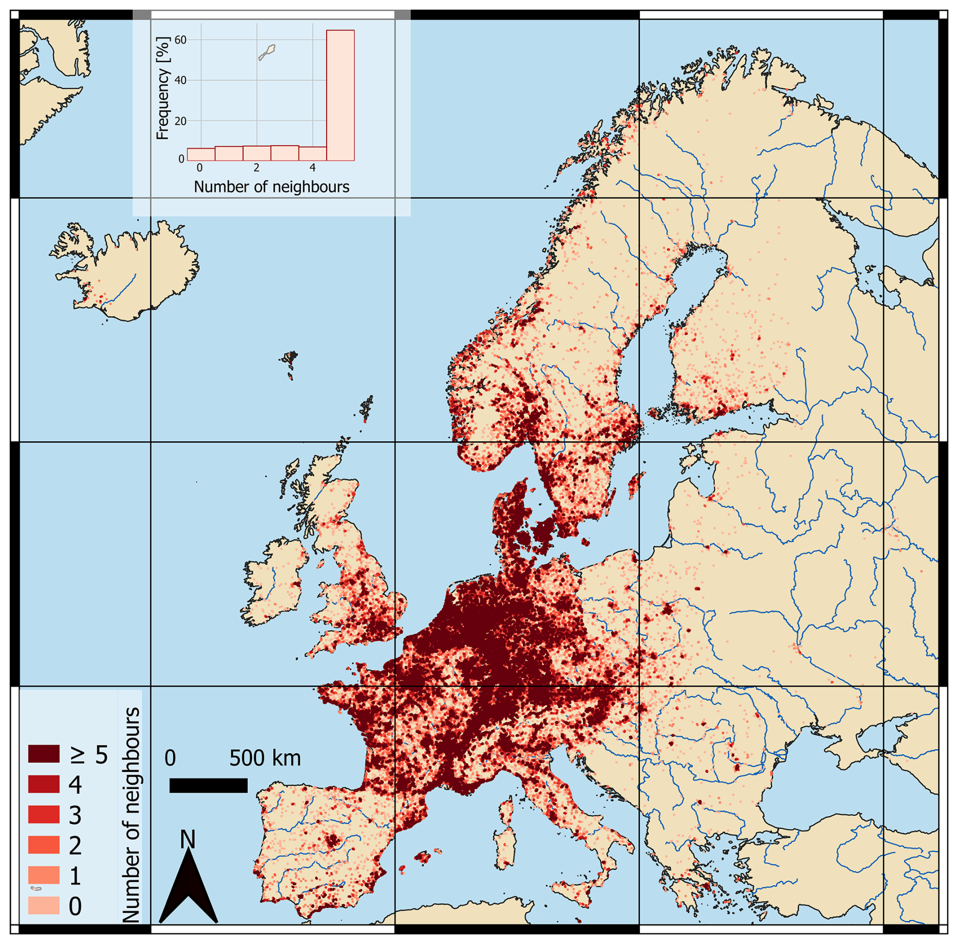
Figure 1 Indication of the density of Netatmo PWSs with rain gauges within Europe, showing the number of PWS neighbours within a radius of 10 km. Data extracted from the Netatmo API in April 2024.

With respect to the PWS-specific sources of error, de Vos et al. (2017) used an experimental setup to investigate part of the instrument-related and data-processing-related errors from PWSs. They showed that, under ideal circumstances (i.e. installed and maintained according to World Meteorological Organization standards), three rain gauges, from the Netatmo brand, recorded rainfall with high accuracy. Collocating the PWSs very close to one of the Royal Netherlands Meteorological Institute (KNMI) AWSs, spatial sampling errors were also limited. Despite the potential of accurate rainfall measurements from PWSs, their observations are often not optimal, as the stations are not necessarily installed according to guidelines from the World Meteorological Organization. For that reason, de Vos et al. (2019) developed a quality control (QC) algorithm to filter outliers from the PWS network without using data from an official rain gauge network or weather radar. Similarly, Bárdossy et al. (2021) developed a QC algorithm using a reference observation network to filter outliers and correct the bias. Chen et al. (2018) assigned trust scores based on spatial consistency between stations.

While previous work has shown that implementing these QC algorithms yields an overall improvement in the quality of the PWS data (de Vos et al., 2019; Bárdossy et al., 2021; Graf et al., 2021; Overeem et al., 2024a; Nielsen et al., 2024; El Hachem et al., 2024), a systematic long-term analysis of the QC algorithm of de Vos et al. (2019) for different seasons, accumulation intervals, and intensity classes has been missing so far. In particular, a focus on high rainfall intensities is important, as the undercatch of rain gauges is likely disproportional with increasing intensities. Here, we aim to quantitatively compare rain data from PWSs and AWSs, expanding on the results of de Vos et al. (2017, 2019). While weather radar data have a higher spatial resolution than AWSs, they are not used in this research as a reference because they are prone to several sources of error and therefore significantly underestimate rainfall. Note that in previous research by Overeem et al. (2024a) and Nielsen et al. (2024), rainfall estimates from PWSs were actually used to correct a rainfall radar product.

The objective of this study is to systematically quantify and describe the uncertainties arising from PWS rainfall estimates. By analysing the 10 largest rainfall accumulations with return periods of up to 50 years during the period between 2018 and 2023, for 11 AWSs, four seasons, and four time intervals, we can draw statistically meaningful conclusions about this. To the best of the authors' knowledge, such a long-term study using PWS data that focuses on the most intense rainfall events has not been performed before. Quantifying the limitations of PWS rainfall observations and addressing them enhances the potential of PWSs for a wide range of applications, including hydrological modelling, urban hydrology, and (hydrological) forecasting.

2 Study area and data

This study was carried out over the period 2018–2023 in the Netherlands, which has a land surface area of approximately 35 000 km² (Fig. 3a). This period was chosen due to the PWS data availability, which was too low (less than five PWSs within a 10 km distance of the AWS) before 2018 and increased over the years. The Netherlands has a maritime climate (Cfb according to the Köppen classification), where winters are mild with an average temperature of 3.8 °C and summers are relatively cool (17.2 °C) (KNMI, 2024). The average yearly rainfall between 1990 and 2020 is 851 mm yr⁻¹ over the area (KNMI, 2024). In addition, regional variability in rainfall extremes is observed, with higher values in the western part of the country (Overeem et al., 2009a; Beersma et al., 2019). The Dutch climate has a quite uniform distribution of precipitation over the meteorological seasons, except during spring, which is the driest season and contains the driest month (i.e. April, average 41 mm) (see Fig. 2). August is on average the wettest month (average 87.4 mm) (KNMI, 2024). However, rainfall characteristics differ over the seasons. Rainfall during the summer months and the beginning of autumn is characterized by shorter durations and higher precipitation intensities as a consequence of convection during these months. In contrast, during the winter months, lower intensities and more frequent and longer precipitation events occur (De Vries and Selten, 2023). These different rainfall characteristics lead to a distinct seasonal cycle in spatial rainfall correlation in the Netherlands (Van de Beek et al., 2012, Fig. 4b), with longer correlation distances for winter than for summer.

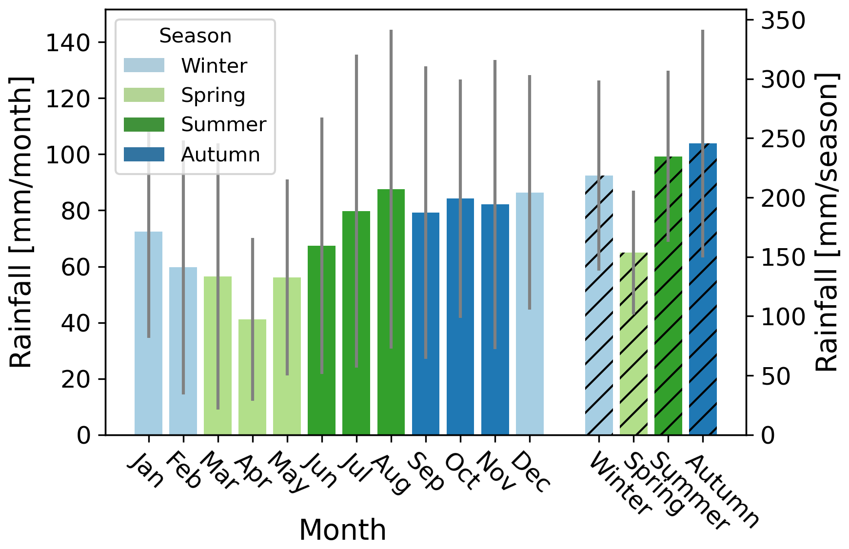
Figure 2 Average rainfall per month and season in the Netherlands over the period 1991–2020, based on data from 13 automatic weather stations spread over the country and obtained from KNMI (2024). Coloured bars indicate the average rainfall per month (millimetres per month, left y axis), and coloured hatched bars indicate the average rainfall for each season (millimetres per season, right y axis). Vertical grey lines indicate the interquartile range.

2.1 Personal weather stations

For the analysis here, rain gauges from the Netatmo brand of PWSs were used. These PWSs have a large coverage over the Netherlands which has slightly increased since 2018 (around one PWS per 9 km² area in 2024; Fig. 3a). This rain gauge type uses a tipping bucket mechanism with a nominal volume of 0.101 mm according to the manufacturer (Netatmo, 2024a). These gauges can also be calibrated manually by the owner by changing – via software – the volume per tip, resulting in deviating tipping bucket volumes (approximately 13.5 % is manually calibrated according to de Vos et al., 2019). The diameter of the collecting funnel is 13 cm (leading to an orifice area of 133 cm²). According to the manufacturer, the accuracy is 1 mm h⁻¹ for a measurement range of 0.2 to 150 mm h⁻¹, and the PWS operates best for temperatures between 0 and 50 °C (Netatmo, 2024a). However, it is unclear what this accuracy exactly entails, thereby showing the need for this study.

The default rain gauge processing software records the number of tips over approximately 5 min intervals, which is communicated wirelessly to an indoor module. Next, the data are transmitted via Wi-Fi to the Netatmo platform. The Netatmo software resamples this to regular 5 min intervals by assigning the data to the next full 5 min interval. When within a 5 min interval no data are transferred, this time interval is not included by Netatmo (see the supporting information in Table A1 for an example). When there is a connection failure between the rain gauge module and the indoor module, the rainfall will likely be attributed to a timestamp when there is a connection again, potentially aggregating it over a longer time interval than approximately 5 min (see the supporting information in Table A2 for an example). However, when the connection of the indoor module is also temporarily interrupted, data are lost.

2.2 Reference dataset

The PWSs were evaluated against data from AWSs from the KNMI. The KNMI operates a network of 33 AWSs across the Netherlands, which are relatively homogeneously distributed with approximately one AWS per 1000 km² area (Fig. 3a). These AWSs estimate cumulative rainfall every 12 s by measuring the displacement of a float placed in a reservoir. The data are archived at a lower resolution, i.e. every 1, 10 min, and hourly. Here, AWS data with resolutions of 10 min and 1 h are used. The 10 min dataset contains unvalidated rainfall data, while the hourly data have been validated (Brandsma et al., 2020). The collecting funnel has a diameter of 16 cm (corresponding to an orifice area of 201 cm²) and the device is heated for temperatures below 4 °C. In addition, these stations are placed in open locations using an English setup or Ott windscreen to reduce errors from wind-induced undercatch (Brandsma et al., 2020). Nevertheless, these data are not an absolute truth. Brandsma (2014) compared the AWS network and manual rain gauge network over the Netherlands and concluded that the AWS network underestimates rainfall at 5 %–8 % annually, with a higher underestimation in winter (7.7 %) than in summer (5.0 %). The undercatch is non-linear with intensity, with larger intensities resulting in less underestimation. These uncertainties are not taken into account in this research.

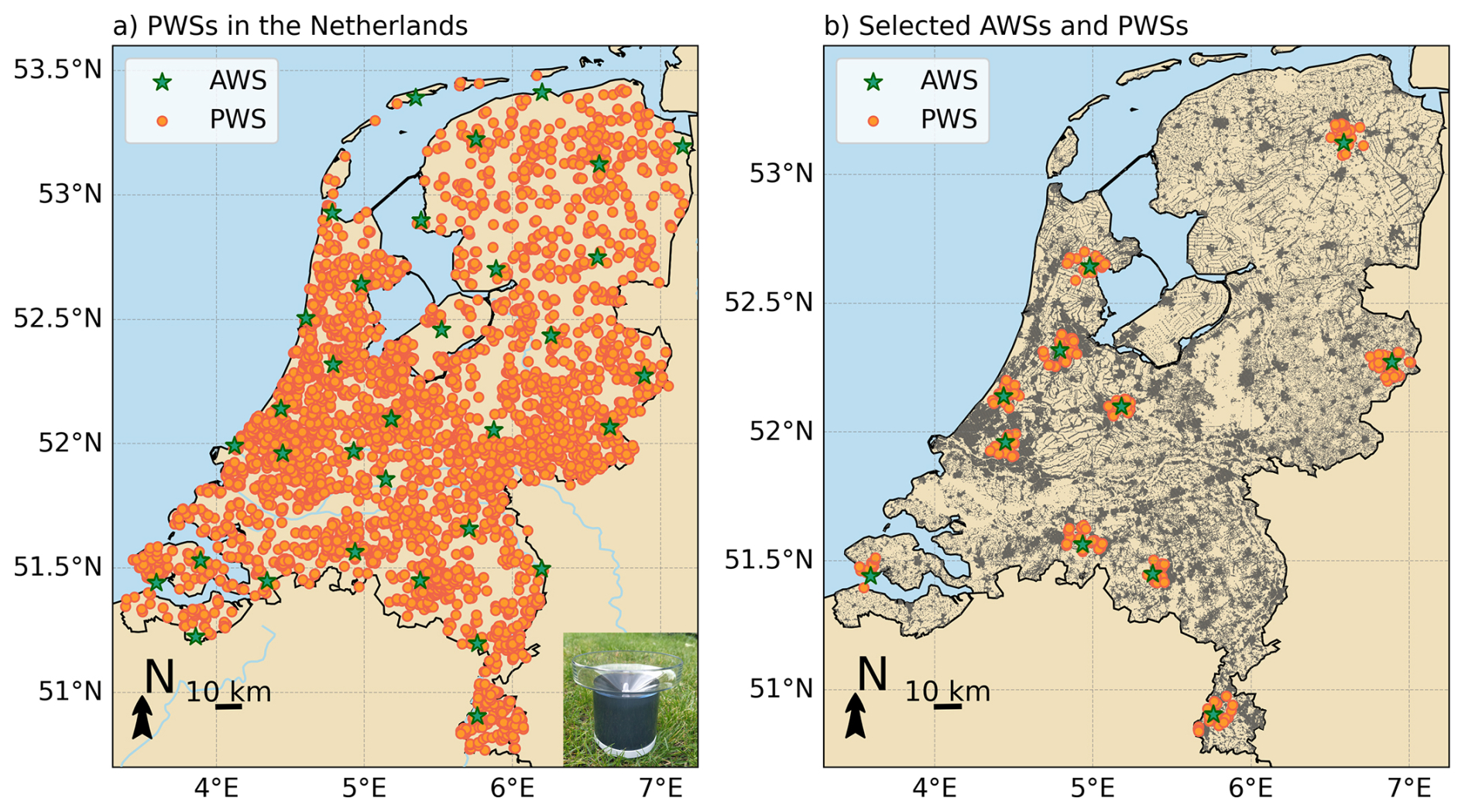
Figure 3 Map of the Netherlands showing (a) the locations of the 33 AWSs employed by KNMI and the locations of available PWSs in 2024 obtained using the Netatmo API (approximately 4000 PWSs) (Netatmo, 2024b). The photo in the right corner shows an example of the PWS used in this research. Note that working PWSs in 2024 are not part of the dataset in this study. (b) The selected AWSs and PWSs from 2018 to 2023 in this study. Built-up areas, indicated in grey, were obtained from the European Environment Agency (2020).

3 Methods

3.1 Station selection

Rainfall data at 5 min intervals from multiple PWSs were extracted using the Netatmo API (Netatmo, 2024b). Note that the API only provides access to data from PWSs that were operational at the time of access, which was in February 2024. We do not have access to data from stations that were previously in operation but no longer online at the time of access. Two search radii were employed to find all operational PWSs within that range. One radius of 10 km around an AWS was used to quantify the quality of the PWSs, and a radius of 20 km was used to filter the PWS data using a quality control algorithm. Van de Beek et al. (2012) and Van Leth et al. (2021) showed that the decorrelation distance for precipitation over the Netherlands is around 50 km for 1 h accumulation intervals. Comparing PWSs within 10 km of an AWS can therefore be assumed to limit spatial sampling errors with respect to a larger search radius.

First, all PWSs within 20 km around each AWS were identified. Second, AWSs that had at least five PWSs within 10 km since 1 January 2018 were kept in the dataset. Next, the 10 closest available PWSs located within 10 km of the AWS were selected (Fig. 4, purple crosses) for the comparison with the AWS nearby. Note that the selection of PWSs varies per selected rainfall event due to temporary station outages and changing data and station availability over time. This procedure resulted in 11 AWSs with a cluster of 5 to 10 PWSs around it (see Fig. 3b for the selected AWSs and the used PWSs). All PWSs within 20 km were used to filter the data (Fig. 4, orange dots and purple crosses) using the quality control algorithm developed by de Vos et al. (2019) and described below (Sect. 3.4).

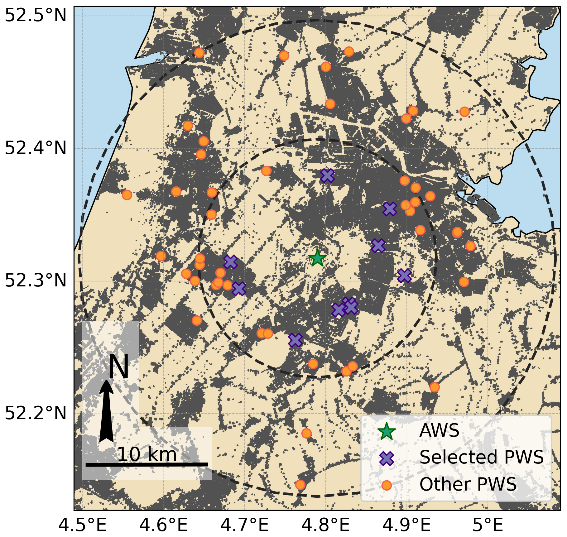
Figure 4 Example of the selection procedure for the AWS at Schiphol. The green star indicates the AWS operated by the KNMI, and the purple crosses indicate the 10 closest PWSs within a distance of 10 km around the AWS. The orange dots are the other PWSs within 20 km of the AWS, which are utilized for quality control. Built-up areas, indicated in grey, were obtained from European Environment Agency (2020).

3.2 Event selection

A similar event selection procedure was used as described by Imhoff et al. (2020), which defines an event as a certain time period rather than by the beginning and end of rainfall. Rainfall observations from the 10 min dataset of the AWSs were employed to make a selection of events between 2018 and 2023 using a moving window approach. Only the 10 largest rainfall accumulations were selected, as these are the most important ones for pluvial flood forecasting. Analysis shows that, on average, the 10 highest 1 h rainfall accumulations for the selected AWSs account for 12.5 % of the annual rainfall. The hourly dataset (clock hour) was employed to perform a consistency check on this selection. For selected events with rainfall differences of more than 10 % with the validated hourly dataset, the values of the validated hourly dataset were used instead. These deviations occurred in less than 0.4 % of the total number of selected events. Note that the selected events can contain time steps without any rain observed.

For every selected AWS based on the methodology in Sect. 3.1, the 10 largest rainfall events per meteorological season (winter, spring, summer, and autumn) and accumulation interval (1, 3, 6, and 24 h) were selected to draw statistically meaningful conclusions. This results in a total of 11 stations × 4 seasons × 4 accumulation intervals × 10 events = 1760 individual events for the analysis. The events were selected in such a way that, for the same station and accumulation interval, no overlapping time series were included.

The statistics of the selected events are shown in Fig. 5. A clear seasonality is observed here, especially for 1 h intervals (Fig. 5a), with the highest rates during summer (June–July–August, JJA) and the lowest rates during winter (December–January–February, DJF) and medians of 14.65 and 6.17 mm h⁻¹, respectively. This is in line with the Dutch climate, where the highest rainfall intensities occur during summer and are typically characterized by convective rainfall (Beersma et al., 2019).

Based on the return periods provided by Beersma et al. (2019), over 75 % of the selected observed rainfall accumulations in winter, spring, and autumn have a return period of less than 0.5 years, while in summer this is around 25 % (Fig. 5a). Most extreme events occur during the summer months, with multiple events having a return period of over 5 years and one event exceeding a return period of 100 years. Rainfall rates during the autumn months (September–October–November, SON) are slightly higher than in spring (March–April–May, MAM), with medians of 9.40 and 8.33 mm h⁻¹, respectively (Fig. 5a). However, spring appears to have two extreme outliers, with return periods that exceed 10 years. Note that these return periods are calculated based on annual statistics, which are dominated by rainfall events from March to October. Because winter has the lowest intensities, return periods then based on annual statistics are low.

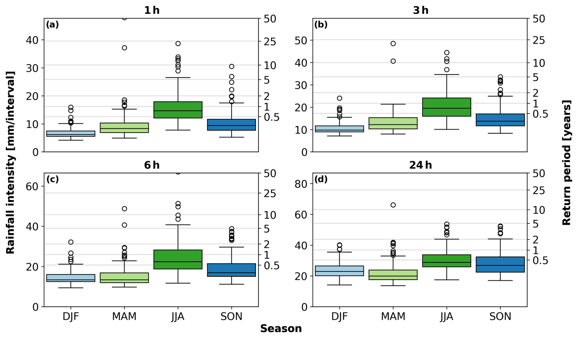
Figure 5 Mean rainfall intensity (millimetres per interval) for the different selected events per season (11 AWSs × 10 rainfall events) for the four accumulation intervals (1, 3, 6, and 24 h). The left y axis shows the rainfall over the specific interval, and the right y axis shows the different corresponding return periods for the intensities reported by Beersma et al. (2019). The lower and upper whiskers indicate the minimum and maximum intensities and the boxes the inter-percentile range (25th–75th). During summer, outliers were present, with return periods longer than 50 years.

3.3 Areal reduction factor

The rainfall observed by a cluster of PWSs is averaged, effectively representing the rainfall over an area while comparing it with a point measurement (AWS), which has a limited spatial footprint. With an increasing domain area, the variation of areal precipitation becomes smaller than that of point precipitation. To account for the reduction in the magnitude of rainfall extremes over an area as compared to a point, areal reduction factors (ARFs) can be applied. The ARF estimates areal rainfall percentiles from point rainfall percentiles. Overeem et al. (2010) and more recently Beersma et al. (2019) parameterized the ARF based on weather radar for the Netherlands. This reduction factor is a function of duration, area, and return period, with rarer events having a stronger areal reduction. Equations (1a), (2), (3b), (4), and (5) of Beersma et al. (2019) are used to estimate the ARF. The inverse of the ARFs will be used to adjust the values of the PWSs to a point observation.

3.4 Quality control algorithm

As stated by El Hachem et al. (2024), the key advantage of the QC algorithm of de Vos et al. (2019) over QC algorithms such as those developed by Bárdossy et al. (2021) and Lewis et al. (2021) is that no auxiliary data are required. This makes it particularly suitable for regions lacking access to (real-time) reference data. For that reason, we decided to use the QC of de Vos et al. (2019). The high-influx (HI) and faulty zero (FZ) filters from the personal weather station quality control (PWSQC) algorithm of de Vos et al. (2019) were applied to filter the PWS dataset. HI data can be caused by sprinklers, addition of liquids into the gauge, or tilting of the gauge. In addition, a high influx can result from a temporary connection interruption between the rain gauge module and the indoor module, assigning the rain to the timestamp when the connection is re-established. Disaggregating this type of high influx using reliable rainfall time series from nearby stations could potentially solve this issue. The HI filter uses four parameters:

1. d, the maximum distance over which neighbouring PWSs are selected that likely capture similar rainfall dynamics;

2. n_stat, the minimum required number of neighbouring PWSs;

3. ϕ_A, a threshold value; and

4. ϕ_B, a threshold value.

A time interval of a station is flagged as having a “high influx” if the median of the neighbouring stations does not exceed ϕ_A, while the station itself records a value above ϕ_B. When the neighbouring stations observe moderate to heavy rainfall, the station is flagged when the measurement exceeds the median × (ϕ_B/ϕ_A). According to de Vos (2019), most rainfall observations that should be flagged by the HI filter were very high. They tested different subsets of parameters and found that variations in ϕ_A and ϕ_B hardly affect the results.

Faulty zeroes can result from failure of the tipping bucket mechanism due to, for example, a tilted rain gauge or obstructions such as leaves or insects. The FZ filter uses three parameters, i.e. the range d, n_stat, and n_int. For the n_int time intervals at least, the median of the neighbouring PWSs needs to be higher than zero, while the PWS itself reports zero rainfall.

The value of parameter d calibrated by de Vos (2019) (Table 1) is 10 km for both HI and FZ. This is the average decorrelation distance of rainfall at the 5 min time interval in the Netherlands (Van Leth et al., 2021, Fig. 4a). This same work shows that this value ranges from about 10 km in summer to about 50 km in winter. In our research, we limit the effect of spatial variability of rainfall by selecting only the five closest neighbouring stations (this is on average a distance of 5.4 km), well within the decorrelation distance of rainfall at the 5 min timescale for any season in the Netherlands (Van Leth et al., 2021).

For the reasons mentioned above, the same calibrated parameters as in Table 2 of de Vos (2019) were applied. First, a list of PWS neighbours within 10 km was constructed. Second, HI and faulty zero FZ filters were computed for every time step (i.e. 5 min). At least five neighbouring PWSs must be present to attribute the HI and FZ flags; otherwise, the value will be eliminated from the dataset. Time steps that were flagged according to the HI or FZ flags were removed.

The station outlier (SO) filter from the PWSQC algorithm requires at least 2 weeks of data (or longer if there was insufficient precipitation in this period) and is computationally expensive, which is not favourable for real-time applications. In addition, by taking the average of a cluster (minimum 5 and maximum 10) of stations around an automatic weather station, the effect of individual station outliers is limited. This last step is different from the method suggested by de Vos et al. (2019). As a last step of the PWSQC algorithm, a default bias correction (DBC) factor was applied to the dataset. de Vos et al. (2017) used an experimental setup and showed that under ideal circumstances there is on average an instrumental bias of 18 % in the Netatmo PWSs, suggesting the need for a DBC factor of 1.22 to correct these instrumental biases.

3.5 Network stability

Over time, the availability of PWSs changes due to factors such as connection failure. To analyse the availability of PWSs, a dataset comprising operational PWSs on 1 January 2018 within 10 km from an AWS was employed. This dataset contained 178 PWSs. Time series from the PWSs were extracted for each selected event according to the method described in Sect. 3.2. In total, 95.8 % of the PWSs were available for all selected events during the 6 consecutive years. From these available PWSs, 3.5 % of the total time steps did not contain any data due to either missing data or irregular data transfers that were longer than 5 min. In addition, 0.7 % of the PWSs did not have five neighbours within 10 km. Applying the quality control algorithm leads to more data being discarded. For the remaining PWSs with enough neighbours, 8.9 % of the total data are either discarded (i.e. flagged as FZ or HI), have a temporal resolution beyond 5 min, or are missing.

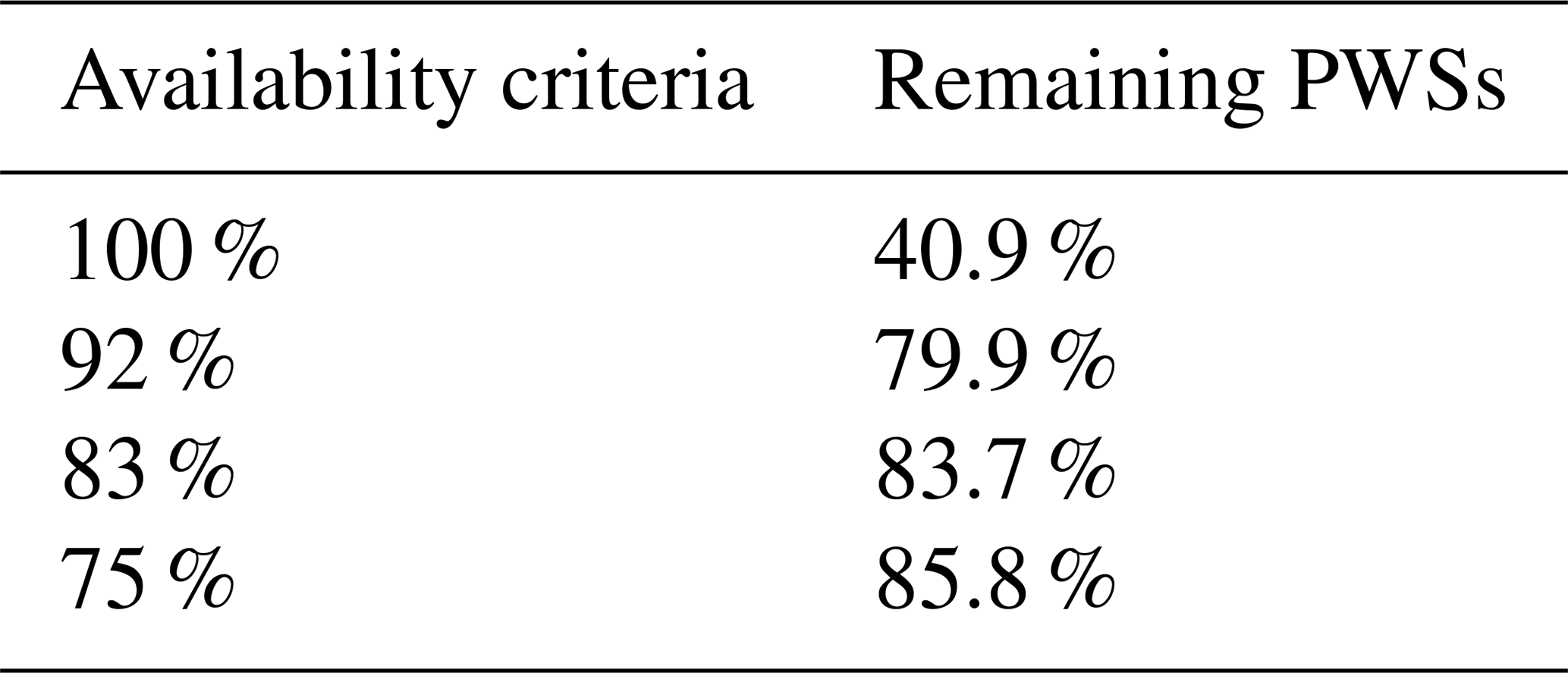
Since we can only suspect that data are likely not missing when a 5 min time step is not included, a minimum availability criterion was set to limit a biased comparison. A minimum percentage of time steps should be valid before aggregating the data. The criterion set has a large impact on the availability (Table 1). By requiring a data availability of 100 % before aggregation, 40.9 % of the dataset is retained, while a lower required availability (92 %) almost doubles (79.7 %) the remaining stations of the original dataset. Lower criteria potentially result in underestimation of rainfall due to missing data. Based on these results, a data availability requirement of 83 % was chosen (e.g. at least 10 out of 12 5 min intervals within 1 h) to keep a large part of the original dataset (83.7 %), which is also in line with Overeem et al. (2024a).

Table 1 Percentage of the PWSs available (28 480 different PWS time series) over all selected events after flagging data and setting minimum availability criteria.

3.6 Validation

The data quality of the PWSs was evaluated by comparing the PWS data to those of the selected AWSs, using the relative bias, the coefficient of variation (CV) of the residuals, the Pearson correlation coefficient (r), and the slope of the linear regression relationship. Note that the evaluation metrics were calculated over the total rainfall within a time interval and over the average of the cluster of PWSs.

The relative bias was defined as follows:

$$\begin{array}{}\text{(1)}& \mathrm{Bias}={\displaystyle \frac{\sum _{i=\mathrm{1}}^n{R}_{\mathrm{PWS},i}}{\sum _{i=\mathrm{1}}^n{R}_{\mathrm{AWS},i}}}-\mathrm{1},\end{array}$$

with n the total number of events for each season and time interval and R_AWS and R_PWS the rain recorded by the AWS and PWS, respectively. Values above zero indicate an overestimation and values below zero an underestimation of the PWS data. The CV is used to describe the dispersion of rainfall, with values closer to zero suggesting greater consistency with the mean of the reference and higher values indicating more dispersion, defined as follows:

$$\begin{array}{}\text{(2)}& \mathrm{CV}={\displaystyle \frac{\sqrt{\frac{\mathrm{1}}{n}\sum _{i=\mathrm{1}}^n{\left(R_{\mathrm{res},i}-{\stackrel{\mathrm{‾}}{R}}_{\mathrm{res}}\right)}^{\mathrm{2}}}}{\stackrel{\mathrm{‾}}{R_{\mathrm{AWS}}}}},\end{array}$$

with the overbar indicating the arithmetic mean and

$$\begin{array}{}\text{(3)}& R_{\mathrm{res}}=R_{\mathrm{PWS}}-R_{\mathrm{AWS}}.\end{array}$$

The Pearson correlation coefficient describes the strength of the linear relation between the PWSs and the AWS, with values ranging between -1 and 1, and it was calculated between all events within a season and aggregation interval (including zeroes):

$$\begin{array}{}\text{(4)}& r={\displaystyle \frac{\mathrm{cov}\left(R_{\mathrm{PWS}},R_{\mathrm{AWS}}\right)}{\mathrm{sd}\left(R_{\mathrm{PWS}}\right)\mathrm{sd}\left(R_{\mathrm{AWS}}\right)}}.\end{array}$$

The linear regression line, fitted through the origin, is defined as follows:

$$\begin{array}{}\text{(5)}& \stackrel{\mathrm{‾}}{R_{\mathrm{PWS}}}=a*\stackrel{\mathrm{‾}}{R_{\mathrm{AWS}}},\end{array}$$

with a the slope calculated over all events:

$$\begin{array}{}\text{(6)}& a={\displaystyle \frac{\sum _{i=\mathrm{1}}^n{R}_{\mathrm{AWS},i}{R}_{\mathrm{PWS},i}}{\sum _{i=\mathrm{1}}^n(R_{\mathrm{AWS},i}{)}^{\mathrm{2}}}}.\end{array}$$

Values close to 1 indicate strong agreement with the reference dataset.

4 Results

After applying the HI and FZ filters and requiring a minimum data availability before aggregation, around 88 % of the original dataset was kept. For 87 (0.5 %) of the total time series used, at least one HI flag was attributed to a time step. In 93 % of the cases, no data were transferred for at least 15 min prior to the flagged HI time step, suggesting that these flags may result from comparing data aggregated over longer time intervals (≥ 15 min) to a 5 min time step, potentially leading to mismatches and flagging data. For 5.8 % of the time series, at least one FZ occurred. Around 15 % of the PWSs were manually calibrated, with a median tipping volume of 0.117 and 95 % of the calibrated tipping bucket volumes ranging between 0.09 and 0.203.

4.1 Spatial sampling

The PWSs in this study were selected based on the closest distance from an AWS without considering the uniformity of the distribution around the AWS. Figure 6 shows that the average cluster distance to an AWS is around 4.4 km and that the average inter-gauge PWS distance of all pairs within a cluster is around 5 km. This indicates that, overall, the selected stations are not clustered in one location and represent a larger area. Variation in the distance to the AWSs in Fig. 6a can be explained by the location of the selected AWSs. Higher PWS network densities and associated shorter distances to the closest PWSs can be found in urban regions. However, most of the AWSs are located in rural regions. In addition, variability in Fig. 6 also partially results from fluctuating data availability and the number of available PWSs, which increases over the years. The average number of PWSs within a cluster is 8.75.

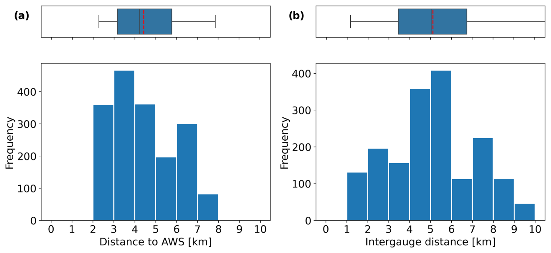
Figure 6 Histogram of (a) the distances between the PWS clusters and the AWSs per event and (b) the inter-station distances between all selected PWS pairs within a cluster per event, all based on 1760 pairs. The vertical red dashed line indicates the mean distance, the vertical black line the median, the left and right whiskers the minimum and maximum distances, and the boxes the inter-percentile range (25th–75th).

4.2 Areal reduction effect

Figure 7 shows a substantial decline in ARFs with larger area sizes and shorter durations, with the largest reductions for short durations. The decline becomes more prominent for longer return periods. For an area of 79 km² (based on a radius of 5 km towards an AWS) and a duration of 1 h, the ARF according to Beersma et al. (2019) varies between 0.88 and 0.82 for return periods of 2 and 50 years, respectively, while for 24 h the ARF varies between 0.96 and 0.92 for return periods of 2 and 50 years, respectively. The reduction becomes larger for a radius of 10 km. For example, the ARFs are 0.78 and 0.70 for a duration of 1 h and return periods of 2 and 50 years, respectively. To convert the areal estimate from the PWSs into a point observation (reflecting the AWS), the PWS cluster average is adjusted using the inverse of the ARF, with the area based on a 10 km radius (the maximum distance between a PWS and an AWS used in the PWS selection procedure).

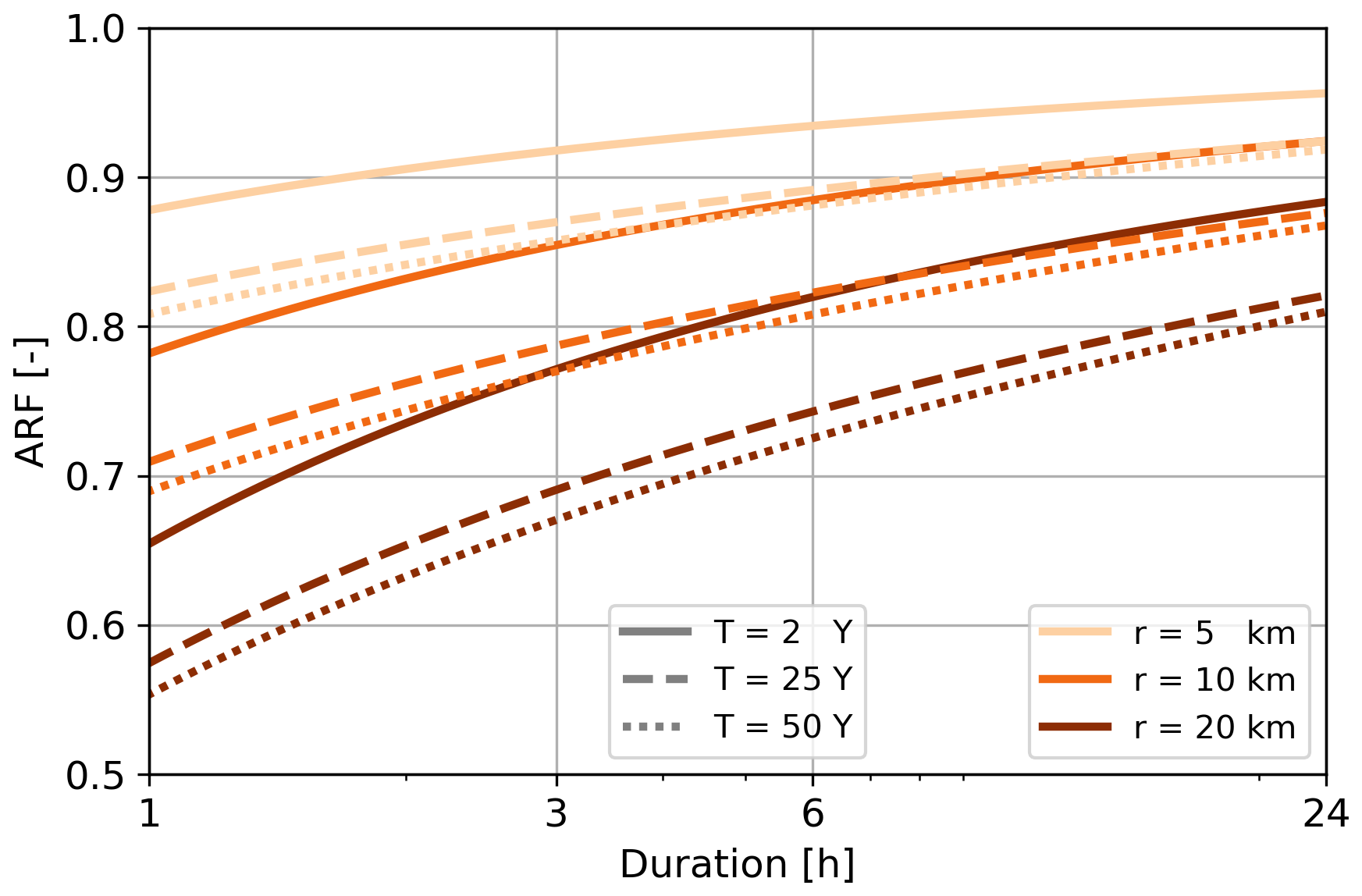
Figure 7 Areal reduction factor (left y axis) as a function of duration for area sizes with radii of 5, 10, and 20 km (converted into an area) and return periods of T=2, 25, and 50 years.

4.3 Bias

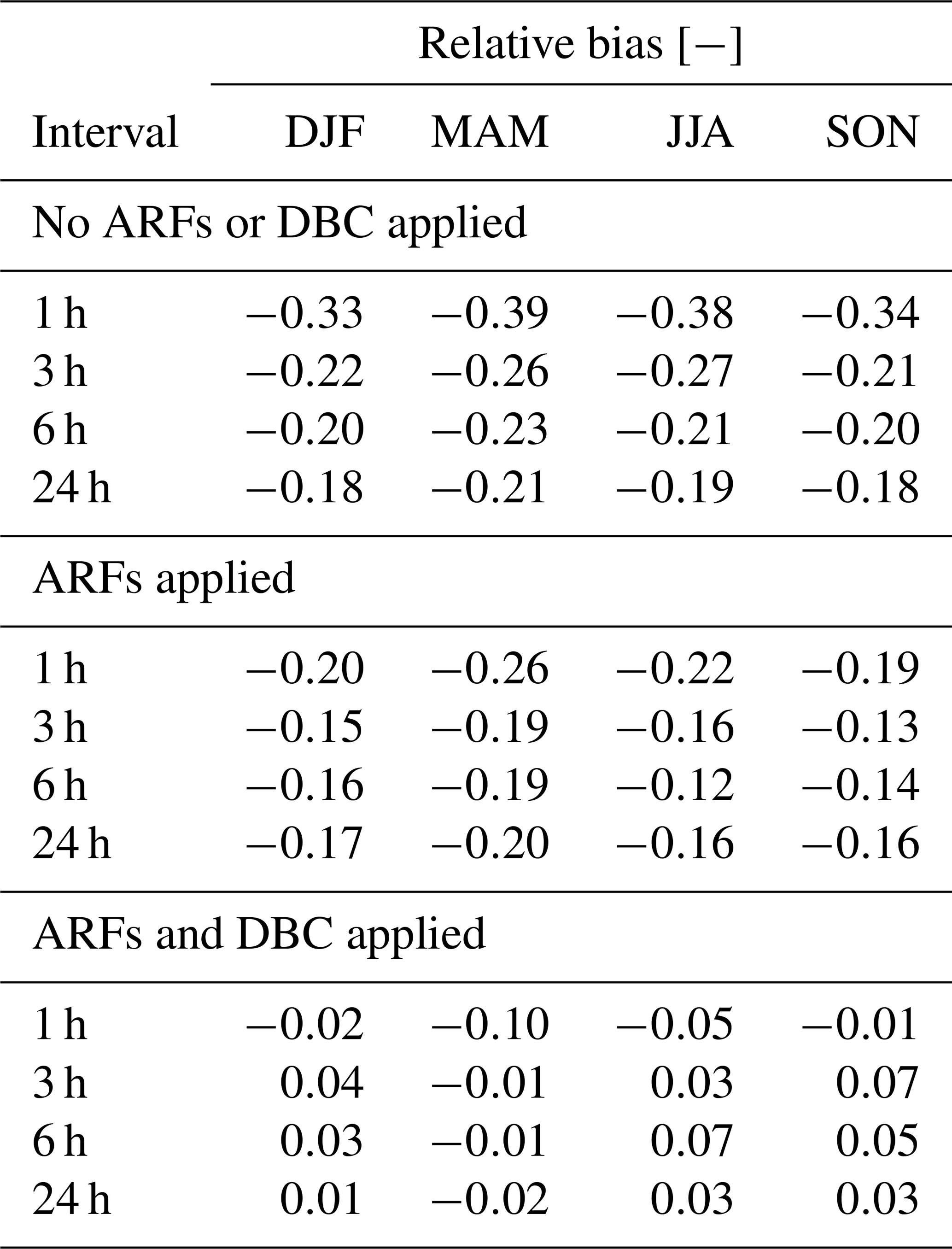
The relative bias of the non-adjusted PWS cluster average over multiple accumulation intervals was quantified by comparing it with AWSs nearby for the selected rainfall events (Table 2, each row indicating different accumulation intervals). Results indicate that, without applying any ARF or DBC factor, on average, significant biases are present in rainfall observations from the PWSs. The underestimation is largest for accumulation intervals of 1 h (around 36 %). The magnitude of the bias decreases over longer intervals towards an average underestimation of around 19 % for accumulation intervals of 24 h. In addition, a seasonal dependency is visible for the bias.

It is important to make a distinction between the sources of bias in order to avoid correcting non-instrumentally related errors. Due to the setup of this study, which makes use of PWSs within a maximum 10 km distance from an AWS, the bias can be divided into two categories: (1) bias resulting from the spatial variation in rainfall extremes and (2) an instrumental bias.

The ARF accounts for the spatial variability of rainfall extremes and illustrates that the bias is partially caused by category 1. The ARF was applied to compensate for the spatial variation of rainfall extremes and to fairly compare the rainfall measured by a cluster of PWSs with one AWS. The largest areal reductions are visible for 1 h accumulation (Fig. 7 and Table 2), reducing the relative bias on average over all seasons from −36 % to −22 %. During the winter months on average, the lowest rainfall intensities and the least spatial variability of rainfall occur (Fig. 9), resulting in the smallest areal reduction. The ARFs have a limited effect on the 24 h events, with an average reduction of 2 percentage points in the bias over all seasons. The remaining bias for time intervals of 3 h over all seasons and longer is on average around 16 %.

The remaining biases are part of the second category and indicate the need for a DBC factor to adjust the instrumental biases. To compensate for this instrumental bias, the DBC factor of 1.22 was applied. After application of this DBC factor, the underestimation for 1 h intervals over all seasons decreases to an average of 5 %, while for 3 h and longer intervals it converges towards zero or in a slight overestimation of the rain. The remaining bias is within the expected uncertainty of rainfall observations. This is supporting evidence that the DBC factor of 1.22 works effectively.

A small part of the dataset obtained from Netatmo (5.38 % of the selected events' total time steps) was not included, suggesting either that data were missing or that the system suffered from connection issues, resulting in irregular data transfer (longer than approximately 5 min). It is expected that the effect of this on the bias will be limited, as most of the data are likely not missing. Rather, the effect is caused by irregular data transfer and/or connection interruption between the rain gauge and the indoor module (see the supporting information in Tables A1 and A2).

Table 2 Relative bias calculated before and after applying an areal reduction factor based on Beersma et al. (2019) and correcting for the instrumental bias over the 110 (i.e. 10 rainfall events × 11 AWSs) selected rainfall events per season and interval.

4.4 Seasonal dependence

For the selected events, a seasonal dependency is visible for the performance of the PWSs (Figs. 8 and 9). The seasonal effect is most pronounced for shorter accumulation intervals (1 h and 3 h), with the best performances of the PWSs in winter and autumn and the worst performances in summer and spring (Fig. 9). Events in winter show the lowest variability of the PWS observations compared with the AWS observations (e.g. average CV values of 0.30 and 0.21 for accumulation intervals of 1 h and 3 h, respectively). While the CV is larger for autumn (0.41 and 0.26), the correlation between the PWSs and AWSs is higher during autumn compared to winter (Fig. 9b). Winter in the Netherlands is mainly characterized by larger, more persistent rainfall systems, which have a longer decorrelation distance (80 km for 1 h aggregations) (Van de Beek et al., 2012). In addition, the error bars for winter are smaller compared with the other seasons, showing that there is more consistency between the individual PWSs (see Fig. 9 and the supporting information in Fig. B1 for a complete overview of all of the seasons and accumulation intervals). For that reason, it is expected that the spatial sampling errors were minimized during winter, indicating that other factors, such as solid rain, caused the lower correlation.

Figure 9a shows that, for all seasons, the CV decreases over longer accumulation intervals. For 1 h intervals the CV varies between 0.30 and 0.54 over the different seasons, while for 24 h the CV shows lower variability, with values varying between 0.14 and 0.27. Similarly, the correlation coefficient increases from values ranging from 0.43 to 0.74 for 1 h intervals to a range from 0.75 to 0.86 for 24 h intervals. This indicates that, for longer accumulation intervals, rainfall observations from PWSs exhibit less variability and more agreement with those from AWSs. Data transferring and processing errors decrease for longer accumulation intervals, as the effect of attributing rainfall to an erroneous time stamp decreases. This takes place for example when the connection between the indoor and outdoor modules is temporarily interrupted, potentially attributing rainfall to a timestamp when there is a connection again and as a consequence aggregating it over a longer time interval than approximately 5 min (see the supporting information in Table A2). Within a cluster of PWSs, variation in rainfall is observed. However, using the average rainfall of each PWS cluster shows great agreement with the AWS. Overall, the average of the cluster of PWSs largely follows the 1:1 line, with slopes of the fitted lines indicating slight underestimation or overestimation by varying between 0.97 and 1.03 for 24 h. A seasonal effect is limited on the slope for durations of 3 h and longer. Furthermore, high correlations, low CV values, and low biases are found for both winter and autumn, indicating that there is good agreement with the AWSs (Fig. 9).

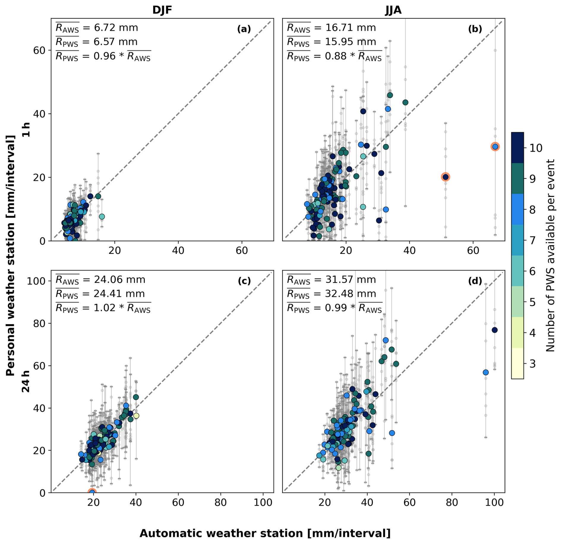
Figure 8 Scatterplots of filtered PWS rainfall accumulations against AWS records for the winter (a, c) and summer (b, d) seasons and accumulation intervals of 1 h (a, b) and 24 h (c, d). The large coloured dots indicate the average of a cluster of PWSs against one AWS, and the vertical bars indicate the minimum and maximum of that cluster of PWSs. The colours indicate the number of PWSs used to calculate the mean, minimum, and maximum rainfall. The small grey dots indicate one individual PWS against an AWS. Orange circles indicate examples of outliers. The $\stackrel{\mathrm{‾}}{R_{\mathrm{AWS}}}$ and $\stackrel{\mathrm{‾}}{R_{\mathrm{PWS}}}$ represent the average rainfall over the selected events recorded by the AWS and PWS, respectively. $\stackrel{\mathrm{‾}}{R_{\mathrm{PWS}}}=a*\stackrel{\mathrm{‾}}{R_{\mathrm{AWS}}}$ represents the linear regression line fitted through zero, with a indicating the slope.

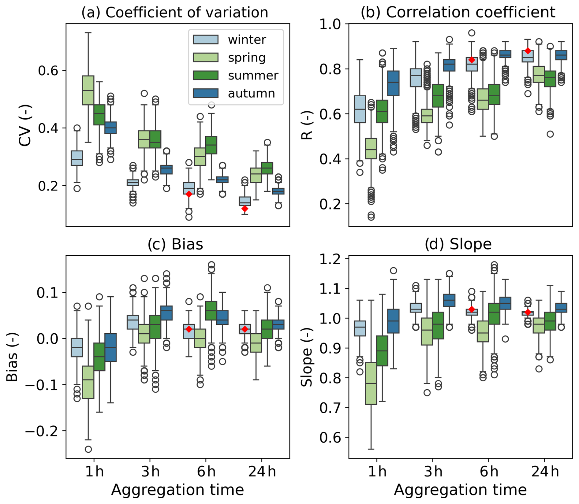
Figure 9 Coefficient of variation (a), correlation coefficient (b), bias (c), and slope (d) of filtered PWS rainfall accumulations against AWS for different seasons and accumulation intervals. The lower and upper whiskers indicate the minimum and maximum of each metric and the boxes the inter-percentile range (25th–75th). The red diamonds indicate the values in winter after discarding events based on attributed temperature flags. The estimated uncertainty is obtained using bootstrapping (1000 iterations with replacement).

4.5 Outlier identification

Figure 8 shows that, for certain individual events, the PWSs report rainfall amounts which deviate strongly from those observed by the AWSs. We investigated the causes of some of these outliers further, which are indicated with orange circles.

It can be seen in Fig. 8c that one of the selected events showed (almost) no precipitation measurements according to the cluster of PWSs, while the AWS nearby recorded precipitation. These outliers occurred during winter and were also observed for the 6 h accumulation interval. In the Netherlands, winter has on average around 34 d with a minimum temperature below 0 °C (KNMI, 2024), which is outside the optimal temperature range of the PWSs. For the event with the outliers in Fig. 8c, the maximum temperature was below −1.4 °C. It is not possible to unambiguously determine whether precipitation is solid based solely on temperature. However, a temperature-based flag can provide end users with an indication that the rainfall observations may be subject to uncertainty. Flags were assigned to time series where the corresponding AWS recorded temperatures below freezing. If these events were discarded by a temperature filter that filters stations when temperatures are below a certain threshold for a certain duration, the values of r and CV for 6 h for winter would have improved to 0.83 and 0.18, respectively. For 24 h this would have been r=0.88 and CV = 0.12. However, as these are only two points and the two intervals have some overlap in time at the same location, no statistically valid conclusion can be drawn from this.

During summer and spring, the highest rainfall accumulations were observed by the AWSs, with intensities exceeding 35 mm h⁻¹. An example of the low performance of PWSs for two high rainfall events in summer can be seen in Fig. 8b. These events likely skew the overall performance during these months. A large spread is observed within the cluster, especially for the highest event in summer in Fig. 8b, indicating a large variation in the spatial rainfall distribution. This suggests that the differences between the cluster of PWSs and AWSs are not necessarily only related to instrumental limitations but are rather due to the spatial rainfall distribution. In addition, tipping bucket mechanisms are known for having difficulties in recording higher rainfall intensities. PWSs only send rainfall data to the Netatmo platform twice every 10 min, which is considerably lower than the recording interval of AWSs (12 s). More than one-third of the rainfall during these events fell within 10 min, exceeding intensities of 75 mm h⁻¹ during that interval. However, it is unknown whether the rain was evenly spread within these 10 min or mostly occurred during a shorter period of time and whether this measurement range of the PWSs was indeed exceeded.

5 Discussion

5.1 Bias

Adjusting the PWS dataset with ARFs and correcting for the instrumental bias using a DBC factor reduces the bias. The remaining bias can indicate either that e.g. a higher DBC factor is required to correct for the substantial underestimation or that the ARFs are not able to fully account for the spatial variability of the rainfall.

5.1.1 Spatial sampling errors

Rainfall exhibits spatial variability, which is related to the temporal scale and rainfall intensity, with shorter temporal resolutions and higher intensities often associated with greater heterogeneity. The decorrelation distance of rainfall is typically much higher in winter compared to summer in the Netherlands. Specifically, for shorter aggregation times, this holds (Van de Beek et al., 2012; Van Leth et al., 2021). The average distance of around 4.4 km from a PWS cluster to the closest AWS was below the decorrelation distance corresponding to a 1 h aggregation interval found by Van Leth et al. (2021) and Van de Beek et al. (2012). While this limits the errors related to spatial sampling, it is expected that this effect will remain most pronounced for events in, for example, summer and spring and at shorter aggregation intervals (i.e. 1 h). Lowering the radius reduces the number of available PWSs and consequently increases the uncertainty. From the error bars in Fig. 8, variation within a cluster of PWSs was observed, with the largest variation found in spring and summer. For small-scale convective rainfall events, the distance to the closest AWS might still have been too large, resulting in the variations in the rainfall observed by the PWSs nearby. Radar images show that, for several events, the differences between AWSs and PWSs are caused by the spatial distribution of the rainfall (see the supporting information in Figs. D1, D2, and D3).

To account for spatial variability, an ARF was estimated for each event. However, such factors are based on areal rainfall climatology, representing an average behaviour and not tied to one specific event. The radius of 10 km, which was based on the maximum possible distance of a PWS to an AWS, was used for the area to estimate the ARFs. For each event, a different PWS cluster was used, potentially representing a larger or smaller area and therefore requiring a different corresponding adjustment of the ARF. A smaller or larger radius has a large effect on the ARF (Fig. 7).

5.1.2 Instrumental bias

An instrumental bias of −18 % was identified by de Vos et al. (2017) using an experimental setup that minimized the spatial sampling errors. This suggests a DBC factor of 1.22 to compensate for the instrumental bias. However, other studies came up with different DBC factors. From de Vos (2019), a bias correction factor of 1.13 came out for a 1-month dataset covering the Netherlands, which is different from the 1-year calibration set from the same study for Amsterdam only (DBC factor of 1.24). Alternatively, Overeem et al. (2024a) used a DBC factor of 1.063 for a pan-European dataset. Neither of the DBC factors (1.063 or 1.13) would have been able to fully compensate for the bias present in the dataset used in this research. This difference might be caused by two main reasons. First, both DBC factors were bulk correction factors tuned on different reference datasets. de Vos et al. (2019) utilized gauge-adjusted radar values. Radars indirectly measure rainfall, which might not be representative of rainfall at the ground. In addition, radars do not measure on a grid. Rather, the values are interpolated, adding extra uncertainty. Spatially adjusting radars with rain gauges improves the overall quality. However, substantial errors remain. Secondly, this research focused on the highest rainfall events over a longer period of time, while neither de Vos et al. (2019) nor Overeem et al. (2024a) distinguished between certain types of rain events, looking rather at a full month or year of rainfall. The performance of tipping buckets is a non-linear function of rainfall intensity (Niemczynowicz, 1986; Humphrey et al., 1997). It requires time for the tipping bucket mechanism to reposition itself after a tip. Higher intensities enhance this problem, resulting in an increased undercatch. Therefore, the type of dataset and the included rainfall events play a role in the performance. Applying a DBC factor of 1.22 over the dataset almost eliminates the bias. The study of de Vos et al. (2017) considered only a few months around the spring period, specifically from 12 February to 25 May 2016, which may have influenced the bias reported in that study.

5.1.3 Manual calibration

Around one-seventh of the PWSs used in this study (15 %) were manually calibrated by their owners. However, it is unknown what the accuracy of such a manual calibration is. The number of tips was determined for each manually calibrated PWS and converted into the original default value of 0.101 mm. On average, there is a 4 % decrease in the rainfall observed by the PWS cluster, resulting in a slightly increased underestimation or slightly decreased overestimation by the PWSs. The CV values slightly improve with an average of 0.01, while the change in r is negligible (see the supporting information in Table C1).

5.2 Quality control

The quality control algorithm of de Vos (2019) utilized in this research improves the overall performance of the PWSs (see the supporting information in Fig. E1). However, there are some limitations to this algorithm. The algorithm works only if there are enough neighbouring stations within 10 km, limiting its usefulness for less densely populated regions. That said, for this study only a small percentage (0.66 %) was discarded from this dataset due to an insufficient number of neighbouring PWSs. While the number of currently active PWSs is quite high in Europe, they are not evenly distributed (see Fig. 1 for the network density of PWSs across Europe). For that reason, regions with a less dense network of PWSs are expected to have a higher percentage of discarded stations due to insufficient neighbours (around 35 % within Europe). Alternatively, other data sources (such as gauges or weather radars operated by national meteorological or hydrological services) can be employed for quality control, such as those employed in the QC algorithm by Bárdossy et al. (2021). In addition, insufficiently calibrated PWSs which record higher rainfall at each time stamp are not discarded by the HI filter if a certain threshold is not reached. These differences become more apparent when accumulated over longer periods. With a dynamic bias correction factor, this could have been adjusted.

Another limitation of a quality control algorithm that does not use auxiliary data is that if all PWSs provide faulty observations, these timestamps are not flagged, consequently giving a wrong signal. This was observed for two events during winter for the 6 and 24 h accumulation intervals, when none of the stations recorded any precipitation during an event, while the AWSs did observe precipitation (e.g. Fig. 8c). During winter, solid precipitation can occur, which can result in an undercatch by the PWSs, as these are not heated and consequently work best for temperatures above the freezing point. Results from Overeem et al. (2024a) also suggested that PWSs are not able to capture solid precipitation. Quality control algorithms based on a reference dataset, such as from Bárdossy et al. (2021), would have filtered these PWSs. Alternatively, a temperature filter could be developed without using auxiliary weather stations. The temperature module present at the PWS can be utilized for this.

6 Conclusions

This study provides insights into the systematic errors across the personal weather station (PWS) network during high-intensity rainfall events by performing a comprehensive analysis over 6 years. The analysis focuses on the most intense rainfall observations for a large number of events (1760) over 6 years (2018–2023) in the Netherlands. PWS data were evaluated against rainfall measurements from automatic weather stations (AWSs). These events were selected over different meteorological seasons (winter, spring, summer, and autumn), durations (1, 3, 6, and 24 h), and AWSs (11 locations spread across the country). PWS data were filtered with a quality control (QC) algorithm utilizing neighbouring PWSs. After QC, around 88 % of the original dataset was kept. To reduce uncertainty from single stations, metrics were calculated over a cluster of PWSs rather than individual stations.

Results showed that PWSs severely underestimate rainfall. A seasonal effect is visible in the bias, specifically for shorter accumulation intervals, with the largest biases for summer and spring. A part of this bias can be attributed to the spatial distribution of rainfall. To account for this, areal reduction factors (ARFs) were applied. This seasonal dependence minimizes after applying ARFs. In addition, a default bias correction (DBC) factor of 1.22 was used to compensate for the instrumental bias. The DBC factor substantially reduces this bias for intervals of 3 h and longer, indicating that the DBC factors of 1.063 proposed by Overeem et al. (2024a) (European dataset) and 1.13 proposed by de Vos et al. (2019) (Netherlands dataset) are not able to account for high-intensity rainfall events. A seasonal and temporal dependence is seen from the correlation coefficient (r) and coefficient of variation (CV). Outliers in winter seemed to have been caused by freezing temperatures (solid precipitation). For that reason, we recommended further analysing the impact of temperature or solid precipitation on the performance of the PWS. The temperature module available in PWSs can be used for this. In addition, PWSs did not observe the most intense rainfall events, with high intensities over a relatively short amount of time (e.g. > 75 mm h⁻¹ within 10 min). These highest intensities occurred during summer and spring, with events that typically occur once in 10 years or even longer return periods. The spatial footprint of these high-intensity rainfall events is often small, influencing errors related to spatial sampling due to the average distance of 4.4 km to the nearest AWS. This suggests the need for a high-density observation network to reliably capture localized rainfall extremes. Rain gauges from the PWSs used in this research utilize a tipping bucket mechanism, which is known to suffer from non-linear underestimation errors with increasing intensities, potentially contributing to these outliers. To quantify this, experimental studies are necessary to limit other sources of errors. The performance of the PWSs improved over longer accumulation intervals, resulting in r values of 0.85 and 0.86 and CV values of 0.14 and 0.18 for 24 h in winter and autumn, respectively.

With the high density of PWSs in the Netherlands (around one PWS per 9 km² area), there is a clear potential to use PWSs. This will also be the case for other regions in Europe that have a relatively high coverage of PWSs. The accuracy however depends on the desired temporal resolution, season, and intensity. Although applying a DBC factor reduces or even completely compensates for the underestimation, we recommend further investigating the dynamic responses of these stations at different intensities to enable dynamic calibration and consequently minimize non-linear errors related to this.

Appendix A: Netatmo data processing

Table A1 Example of the Netatmo software that resamples data to regular 5 min intervals by assigning them to the next full 5 min interval.

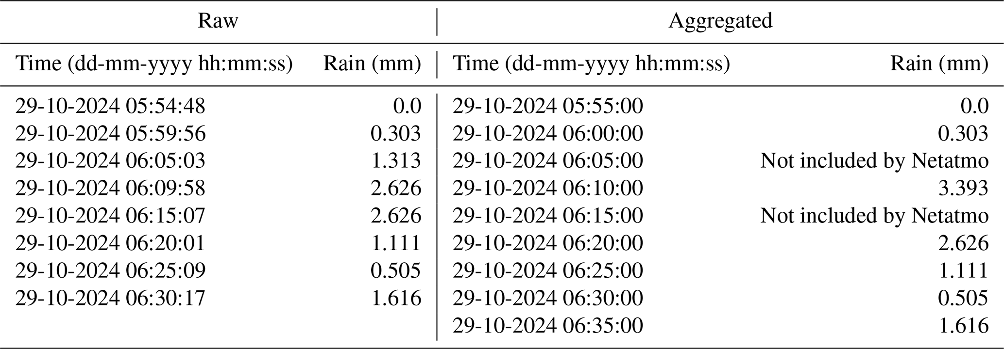
Table A2 Examples of times when there was likely a temporary connection interruption between the indoor module and the rain gauge. Rainfall will likely be attributed to a timestamp when there is a connection again, resulting in a higher temporal resolution. For example, at 20:26:21 the rainfall is likely aggregated over 22 min.

Appendix B: Overview of all seasons and accumulation intervals

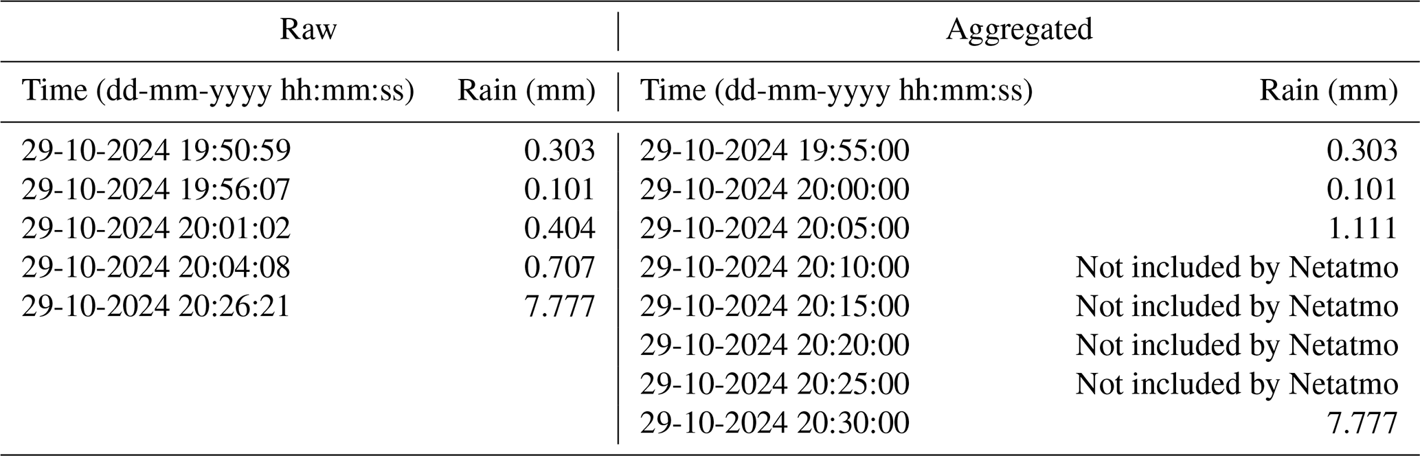
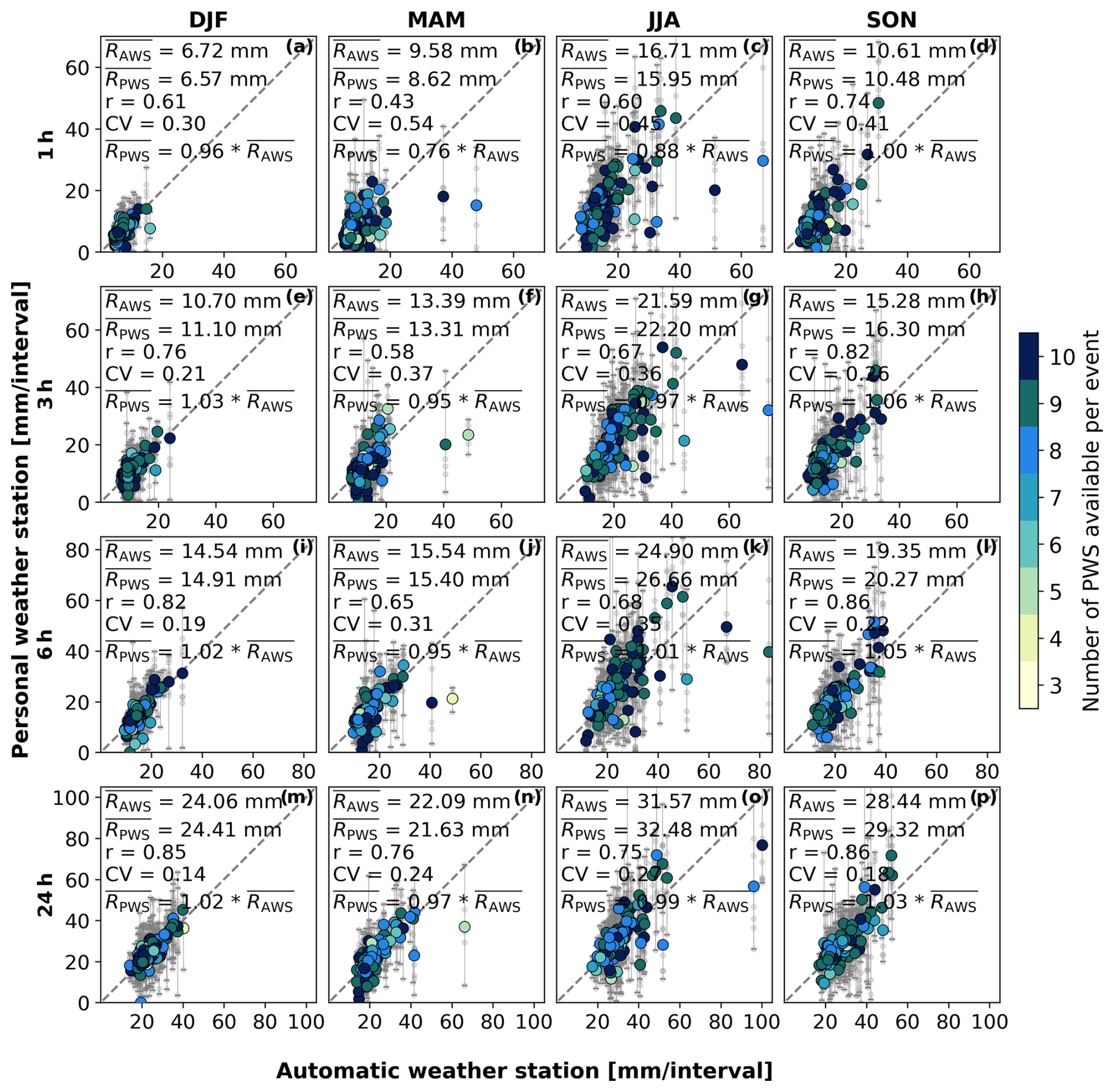
Figure B1 Scatterplots of filtered PWS rainfall accumulations against AWSs for the winter (a, e, i, m), spring (b, f, j, n), summer (c, g, k, o), and autumn (d, h, l, p) seasons and accumulation intervals of 1 h (a–d), 3 h (e–h), 6 h (i–l), and 24 h (m–p). The large coloured dots indicate the average of a cluster of PWSs against one AWS, and the vertical bars indicate the minimum and maximum of that cluster of PWSs. The colours indicate the number of PWSs used to calculate the mean, minimum, and maximum rainfall. The small grey dots represent one individual PWS against an AWS. $\stackrel{\mathrm{‾}}{R_{\mathrm{AWS}}}$ and $\stackrel{\mathrm{‾}}{R_{\mathrm{PWS}}}$ represent the average rainfall over the selected events recorded by the AWS and PWS, respectively. $\stackrel{\mathrm{‾}}{R_{\mathrm{PWS}}}=a*\stackrel{\mathrm{‾}}{R_{\mathrm{AWS}}}$ represents the linear regression line fitted through zero, with a indicating the slope.

Appendix C: Calibration effect

Table C1 Relative bias, coefficient of variation (CV), and correlation (r) of filtered PWS rainfall accumulations against AWSs for different seasons and accumulation intervals. PWSs with manual calibrated tipping volumes were converted into the original default value of 0.101 mm.

Appendix D: Spatial distribution of rainfall

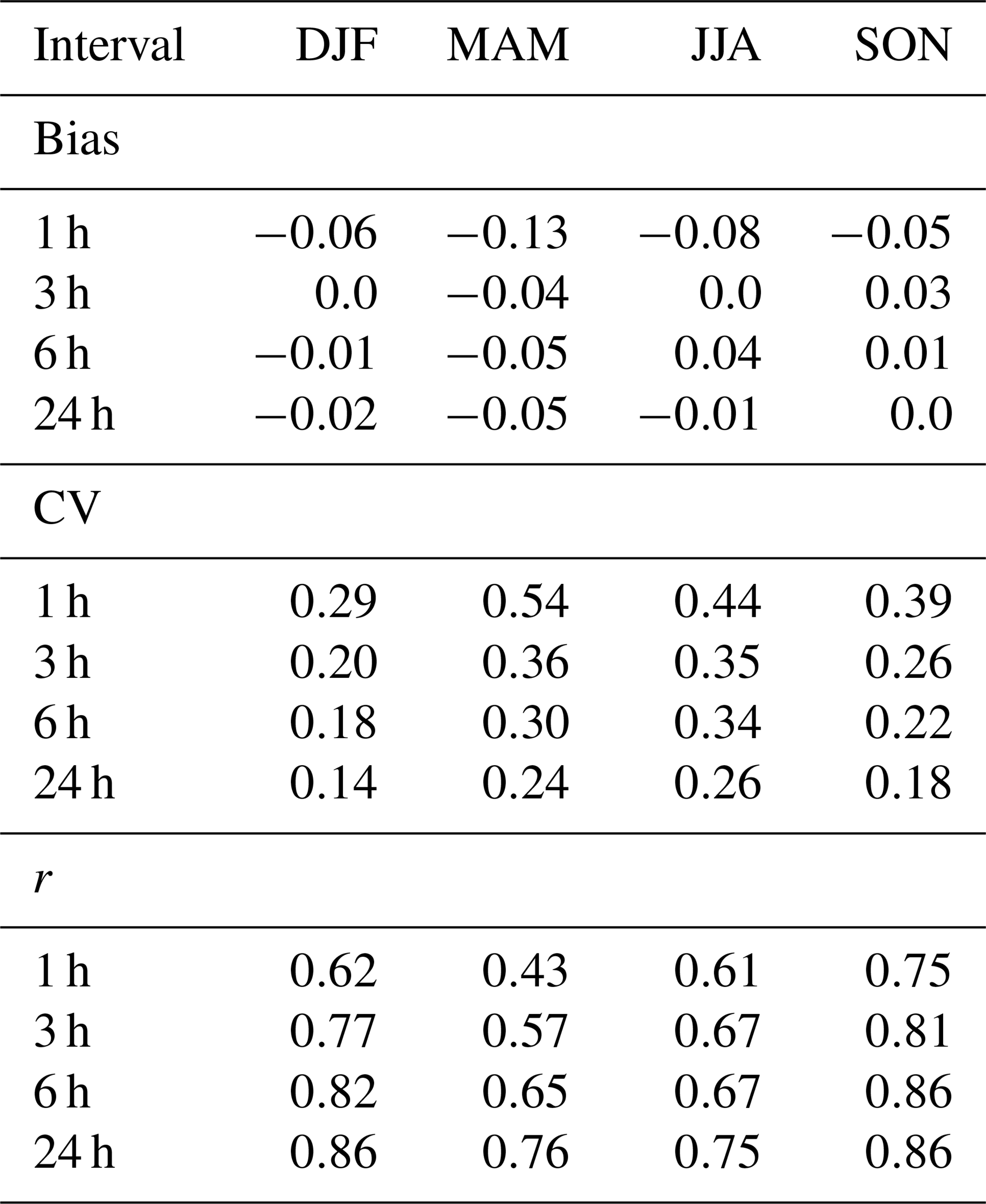
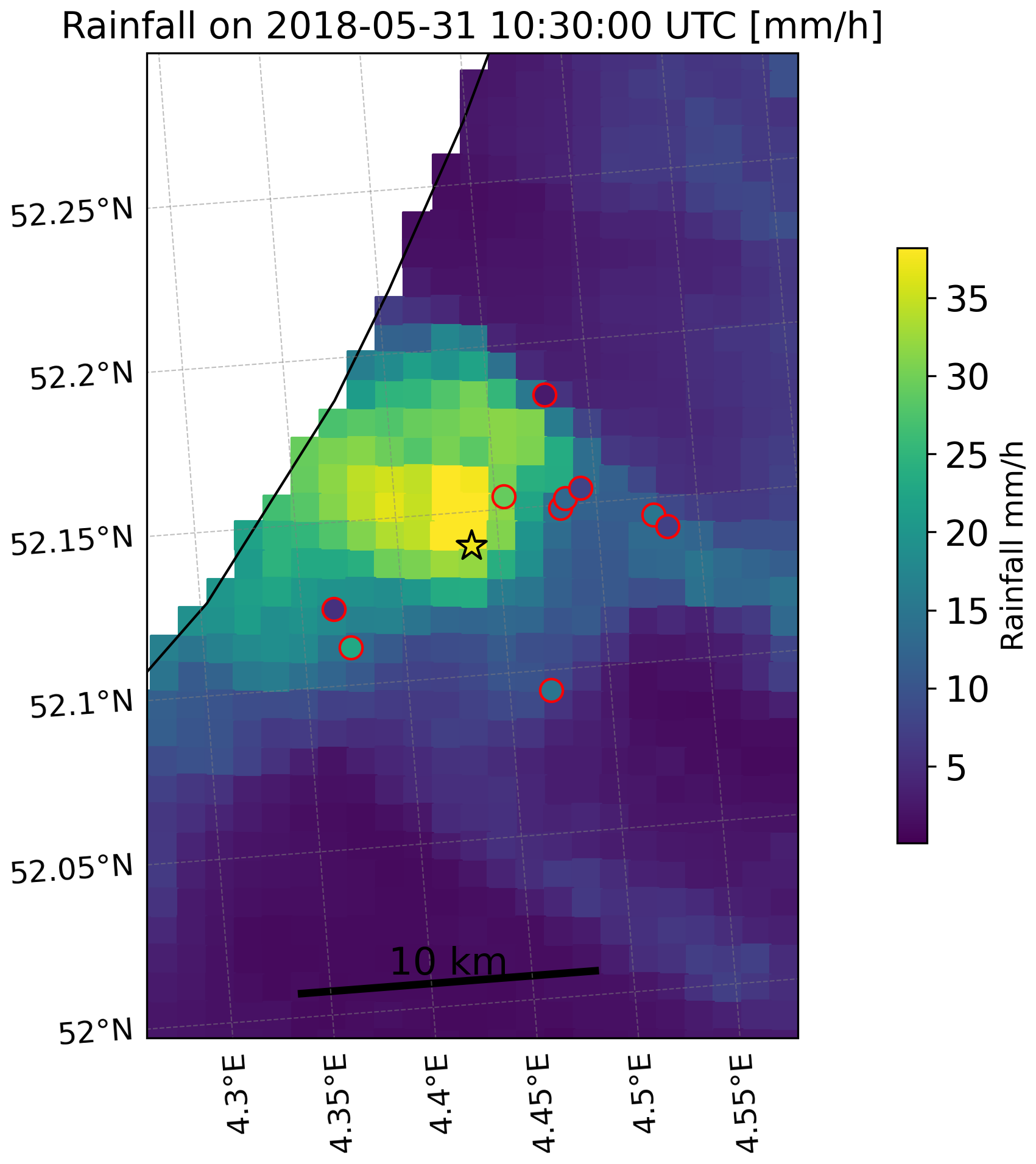
Figure D1 Rainfall distribution on 31 May 2018 at 10:30 UTC, based on 1 h of accumulated rainfall from the gauge-adjusted radar product (Overeem et al., 2009b). The asterisk indicates the location of the AWS which measured 39 mm in 1 h, whereas the circles with red borders represent the locations of the PWSs. The fill colour of both the asterisk and the circles represents the recorded rainfall at the specific rain gauge.

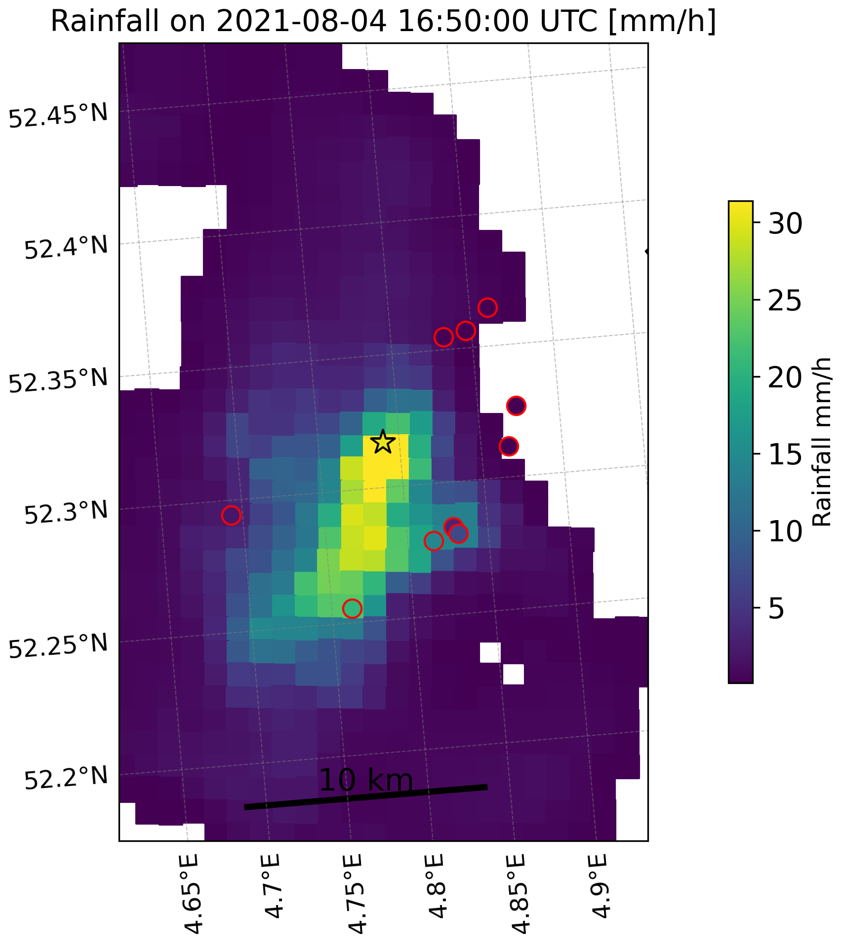
Figure D2 Rainfall distribution on 4 August 2021 at 16:50 UTC, based on 1 h of accumulated rainfall from the gauge-adjusted radar product (Overeem et al., 2009b). The asterisk indicates the location of the AWS which measured 30 mm in 1 h, whereas the circles with red borders represent the locations of the PWSs. The fill colour of both the asterisk and the circles represents the recorded rainfall at the specific rain gauge.

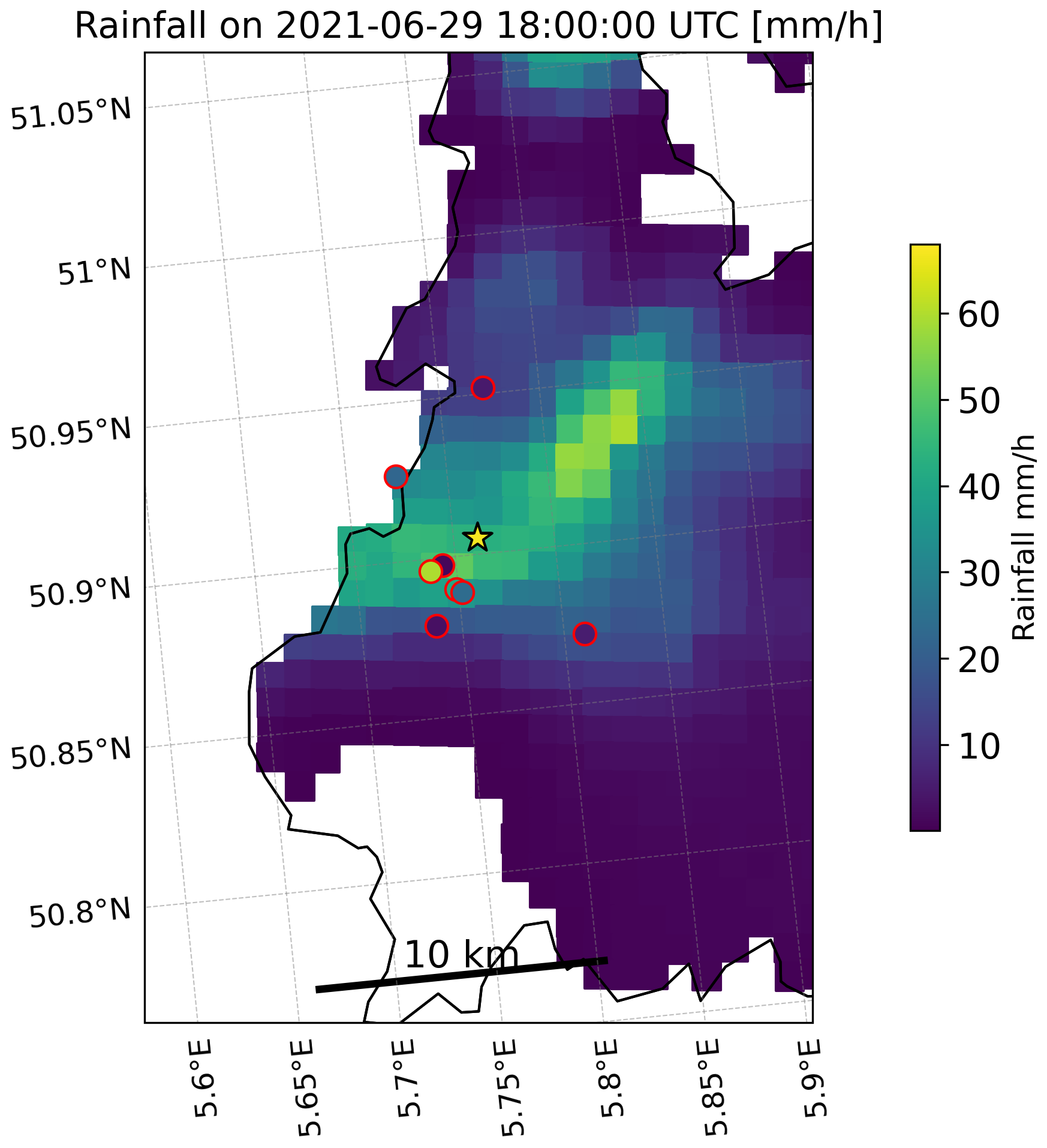
Figure D3 Rainfall distribution on 29 June 2021 at 18:00 UTC, based on 1 h of accumulated rainfall from the gauge-adjusted radar product (Overeem et al., 2009b). The asterisk indicates the location of the AWS which measured 67 mm in 1 h, whereas circles with red borders represent the locations of the PWSs. The fill colour of both the asterisk and the circles represents the recorded rainfall at the specific rain gauge.

Appendix E: Raw PWS data

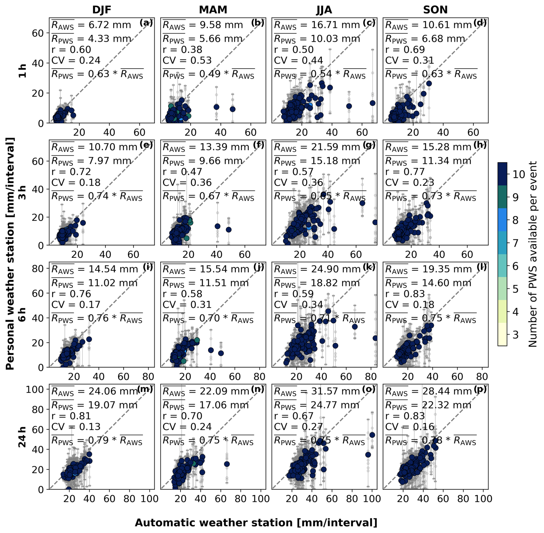
Figure E1 Scatterplots of raw PWS rainfall accumulation data against AWSs for the winter (a, e, i, m), spring (b, f, j, n), summer (c, g, k, o), and autumn (d, h, l, p) seasons and accumulation intervals of 1 h (a–d), 3 h (e–h), 6 h (i–l), and 24 h (m–p). The large coloured dots indicate the average of a cluster of PWSs against one AWS, and the vertical bars indicate the minimum and maximum of that cluster of PWSs. The colours indicate the number of PWSs used to calculate the mean, minimum, and maximum rainfall. The small grey dots represent one individual PWS against an AWS. $\stackrel{\mathrm{‾}}{R_{\mathrm{AWS}}}$ and $\stackrel{\mathrm{‾}}{R_{\mathrm{PWS}}}$ represent the average rainfall over the selected events recorded by the AWS and PWS, respectively. r and CV indicate the correlation coefficient and the coefficient of variation. $\stackrel{\mathrm{‾}}{R_{\mathrm{PWS}}}=a*\stackrel{\mathrm{‾}}{R_{\mathrm{AWS}}}$ represents the linear regression line fitted through zero, with a indicating the slope.