Interrogating process deficiencies in large-scale hydrologic models with interpretable machine learning

Large-scale hydrologic models are increasingly being developed for operational use in the forecasting and planning of water resources. However, the predictive strength of such models depends on how well they resolve various functions of catchment hydrology, which are influenced by gradients in climate, topography, soils, and land use. Most assessments of hydrologic model uncertainty have been limited to traditional statistical methods. Here, we present a proof-of-concept approach that uses interpretable machine learning techniques to provide post hoc assessment of model sensitivity and process deficiency in hydrologic models. We train a random forest model to predict the Kling–Gupta efficiency (KGE) of National Water Model (NWM) and National Hydrologic Model (NHM) streamflow predictions for 4383 stream gauges in the conterminous United States. Thereafter, we explain the local and global controls that 48 catchment attributes exert on KGE prediction using interpretable Shapley values. Overall, we find that soil water content is the most impactful feature controlling successful model performance, suggesting that soil water storage is difficult for hydrologic models to resolve, particularly for arid locations. We identify nonlinear thresholds beyond which predictive performance decreases for NWM and NHM. For example, soil water content less than 210 mm, precipitation less than 900 mm yr⁻¹, road density greater than 5 km km⁻², and lake area percent greater than 10 % contributed to lower KGE values. These results suggest that improvements in how these influential processes are represented could result in the largest increases in NWM and NHM predictive performance. This study demonstrates the utility of interrogating process-based models using data-driven techniques, which has broad applicability and potential for improving the next generation of large-scale hydrologic models.

1 Introduction

Large-scale hydrologic models are important tools for understanding and forecasting the fluxes of water across the earth's surface to manage floods, droughts, and other hydrologic extremes (Brunner et al., 2021; Tijerina et al., 2021). Most often, these models convert meteorological inputs to streamflow predictions by parameterizing and calibrating internal hydrological processes. Accurate simulation of internal processes is a grand challenge of hydrology (Blöschl et al., 2019) because of the difficulty of resolving equifinality (Vrugt and Beven, 2018), scaling relationships (Savenije, 2018), epistemic uncertainties in hydrologic data (Beven, 2024), and spatial heterogeneity in watershed attributes (Santos et al., 2025). The accurate determination of sensitive model parameters and drivers is crucial for improving process representation in hydrologic models and, ultimately, the management of water resources (Pandit et al., 2025; Reinecke et al., 2025).

The National Water Model (NWM) and the National Hydrologic Model (NHM) are two process-oriented, continental-scale hydrologic models used in operational decision-making (Towler et al., 2023). The NWM framework applies the Weather Research and Forecasting Hydrologic model (WRF-Hydro) formulation, which simulates infiltration, evaporation, transpiration, overland flow, shallow subsurface flow, baseflow, channel routing, and passive reservoir routing but not active reservoir management (Cosgrove et al., 2024). The NHM framework applies the Precipitation–Runoff Modeling System (PRMS) formulation, which represents evaporation, transpiration, runoff, infiltration, interflow, groundwater flow, and channel routing but not reservoir operations, water withdrawals, or stream releases (Regan et al., 2019). See Sect. S1 in the Supplement for more details on each model. A key distinction is that the NWM targets high-spatial-resolution (∼ 250 m) and high-temporal-resolution (hourly) flood forecasting. In contrast, the NHM assesses long-term water availability at hydrologic-response-unit scales (∼ 100 km², driven by daily forcing) (Towler et al., 2023). Both models exhibit spatially variable streamflow skill across US catchments (Tijerina et al., 2021), with the strength of prediction varying as a function of catchment-scale climate, land use, and physiography. Collectively, differences in resolution, process formulation, and treatment of human regulation make the NWM–NHM pair an ideal testbed for structural sensitivity analysis: drivers influential in both frameworks likely denote overarching hydrologic controls, whereas divergent sensitivities flag processes that are represented differently (or omitted) in either approach.

The sensitivity of process-based hydrologic models to certain catchment attributes and parameters has been interrogated using well-established statistical tools, such as sensitivity analysis (Pianosi et al., 2016; Song et al., 2015). These approaches work by exploring the range of values that model parameters may take and recording the net impact on model performance (Mai, 2023). Notable examples include the Sobol' (2001) and Morris (1991) methods. A drawback of traditional sensitivity analysis methods, particularly when applied to large-scale hydrologic applications (Mai et al., 2022), is that they can be computationally demanding (Sarrazin et al., 2016). Less demanding techniques, such as the Robustness Assessment Test (RAT; Nicolle et al., 2021), have been developed to evaluate model bias without the need to control the calibration process, but these focus only on the influence of temporal forcings, such as air temperature. Thus, there is a need to continue to develop spatial methods for assessing model sensitivity that are useful in scenarios where traditional methods are computationally intractable.

Explainable or interpretable machine learning methods have the potential to bridge the gap between data-driven insights (provided by machine learning models) and process-based understanding (contained within physically based models) (Slater et al., 2025). These methods help to explain why a model gives the prediction that it does (Lundberg et al., 2020). Several explainable machine learning methods have been developed, including Partial Dependence Plots (PDP; Friedman, 2001), Local Interpretable Model-Agnostic Explainers (LIME; Ribeiro et al., 2016), and Shapley Additive Explanations (SHAP; Lundberg et al., 2020). In hydrology, for example, these tools have been applied for the analysis of hydrologic fluxes (Brêda et al., 2024), soil moisture (Huang et al., 2023), water table depth (Ma et al., 2024), and drought intensity (De Meester and Willems, 2024). Interpretable machine learning can complement and enhance traditional sensitivity approaches (Maier et al., 2024) by providing post hoc interpretative insights into how parameter changes influence hydrologic model predictions – that is, without the need for perturbing the model parameter space. Interpretable machine learning methods are not without limitations as they only imply relations in the model which may not necessarily be causal (Heskes et al., 2020), and thus caution should be exercised when interpreting model explanations.

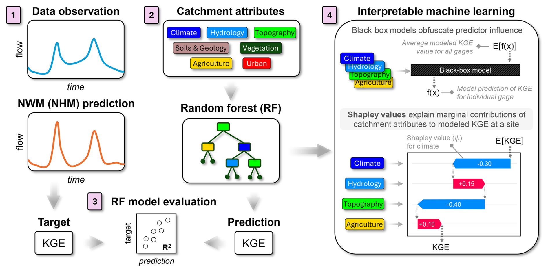
Figure 1 Flow diagram showing the application of interpretable machine learning in this study. (1) Data observations and National Water Model (NWM) or National Hydrologic Model (NHM) predictions are used to generate a target Kling–Gupta efficiency (KGE) for each site. (2) Catchment attributes are input to a random forest (RF) model to predict KGE for each site. (3) The RF model is evaluated by comparing the predicted KGE to the target KGE using the coefficient of determination (R²) to determine goodness of fit. (4) Shapley values (ψ) are used to explain the marginal contributions of catchment attributes that distinguish KGE prediction at a particular site, f(x), from the average modeled KGE for all sites, E[(f(x)]. In the given example, the values of the climate and topography attributes at this individual gauge lower the predicted KGE (−ψ), whereas the values of the hydrology and agriculture attributes increase the predicted KGE (+ψ).

This paper aims to interrogate large-scale hydrologic model performance with machine learning tools to identify which processes may be inadequately represented in physically based models. Thus, the questions we address are the following: what catchment attributes can be used to predict poor model performance, and are certain dominant hydrological processes associated with these catchment attributes? To answer these questions, we present a proof-of-concept approach that uses machine learning techniques to provide post hoc assessment of model sensitivity. We did this by building a random forest model to predict KGE values for NWM and NHM predictions at over 4000 basins (Fig. 1). Thereafter, model predictions were interpreted using Shapley values, which highlight the physiographic and hydrologic controls of process-based model performance. This work aims to inform improvements for the next generation of large-scale hydrologic models for the responsible stewardship of water resources into an uncertain future.

2 Methods

2.1 The National Water and National Hydrologic Model

We retrieve daily streamflow observations and predictions for gauged locations (sites) for the NWM version 2.1 and NHM version 1.0 from existing repositories (Johnson et al., 2023b; Regan et al., 2019; Towler et al., 2023). Section S1 summarizes the models that produced the data used in this study. A total of 4614 basins with at least 10 years of data that span the contiguous US (CONUS) are included in our analysis (USGS Water Data for the Nation, 2023). The date range of flow observations and predictions is from water years 1984 to 2016.

NWM and NHM performance at each site was assessed using the Kling–Gupta efficiency (KGE), a common metric in hydrologic modeling (Gupta et al., 2009). The KGE is calculated as

$$\begin{array}{}\text{(1)}& \mathrm{KGE}=\mathrm{1}-\sqrt{{\left(\mathit{\alpha }-\mathrm{1}\right)}^{\mathrm{2}}+{\left(\mathit{\rho }-\mathrm{1}\right)}^{\mathrm{2}}+{\left(\mathit{\beta }-\mathrm{1}\right)}^{\mathrm{2}}},\end{array}$$

where ρ is the Pearson correlation coefficient, and α and β are the ratios of the standard deviation and the mean, respectively, of model predictions to data observations. The accuracies of NWM (Fig. 2) and NHM (Fig. S1) predictions are particularly sensitive to aridity. The KGE values calculated in Eq. (1) serve as the target variables for the forthcoming machine learning model (Fig. 1).

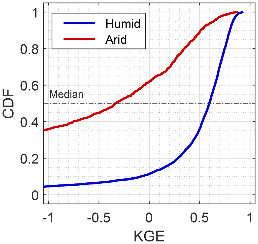
Figure 2 Cumulative distribution function (CDF) of National Water Model (NWM) performance for humid ($\mathrm{PET}/P<\mathrm{1}$, n = 3827) and arid ($\mathrm{PET}/P>\mathrm{1}$, n = 787) sites as assessed by the Kling–Gupta efficiency (KGE) evaluation metric.

2.2 Random forest model

Random forest modeling is an ensemble-based machine learning approach for predicting continuous values and capturing nonlinear trends in a dataset (Ho, 1998). We train a random forest model, comprised of 1000 regression trees, to predict the target KGE at each site using catchment attributes as input variables (termed “features”). The features (n = 48) are derived from BasinATLAS (Linke et al., 2019) and incorporate wide ranges of climate, hydrology, topography, soils and geology, undeveloped vegetation, agriculture, and urban land use. The names and descriptions of the 48 predictors can be found in Table S1, and the spatial variations of the 48 predictors across the CONUS are shown in Fig. S2. The features were selected based on their likelihood to impact hydrology. Soil water content appears to be an important predictor in the later analysis, and we define it here for clarity. Soil water content is defined as the annual soil water available for evapotranspiration (Global High-Resolution Soil-Water Balance, 2023), and the original study authors calculated it as equal to the long-term effective precipitation minus the sum of actual evapotranspiration and runoff.

The random forest model was trained and validated using bootstrapping. Individual trees are grown from an in-the-bag bootstrap of the observation dataset. Out-of-bag observations not included in the bootstrap are used for model validation. The models were trained using the mean squared error objective function. The coefficient of determination (R²) was calculated to assess the predictive performance of the random forest (Pearson, 1901). Extreme values (outliers) can distort the utility of a predictive and interpretable model (Liu et al., 2018). Because the KGE metric has a small upper bound (+1) and an infinite lower bound (−∞), a small subset of very negative values can dominate model inferences. The lowest KGE value for a gauged location in the NWM dataset is −302.8, whereas the 5th percentile of KGE values −2.7. The performance at both sites would be considered “unacceptable”; thus, including extreme negative values negatively affects model predictability without providing much additional insight beyond that given by other underperforming sites. To address the disproportionate influence of a small subset of values, we consider the 5 % of sites with the most negative target KGE values to be outliers, reducing our dataset from 4614 to 4383 sites. Random forest model analyses and development were performed using the TreeBagger function in MATLAB 2024.

2.3 Shapley values

Shapley values are derived from cooperative game theory and they aim to assess how coalitions form and how these coalitions impact the payout of a game (Shapley, 1953). In the context of interpretable machine learning, they are a model-agnostic approach that attributes each feature an importance value for a prediction, indicating the marginal benefit that the inclusion of the feature provides to the overall prediction (Lundberg et al., 2020; Lundberg and Lee, 2017). Thus, Shapley values explain the inner workings of a model, with influential features receiving large attribution of credit, whereas non-influential features may receive little or no credit for the model prediction. The Shapley value is also the only distribution of gain among features (e.g., predictor variables) that satisfies four properties: (1) efficiency, (2) symmetry, (3) linearity, and (4) null player (Shapley, 1953). These properties respectively ensure that (1) the total prediction is fully allocated to features, (2) features that contribute the same to the prediction should receive identical credit, (3) the feature attribution for a model that combines several sub-models should be the sum of the attributions from each sub-model, and (4) a feature contributing nothing to the prediction should receive no allocation.

The Shapley value (ψ) of the ith feature (catchment attribute) for the query point x (KGE) can be calculated by the characteristic value function (v) as

$$\begin{array}{}\text{(2)}& \begin{array}{rl}{\mathit{\psi }}_i\left(v_x\right)=& {\displaystyle \frac{\mathrm{1}}{M}}\sum _{S\subseteq N/\mathit{\left\{}i\mathit{\right\}}}{\displaystyle \frac{\left|S\right|\mathrm{!}\left(M-\left|S\right|-\mathrm{1}\right)\mathrm{!}}{\left(M-\mathrm{1}\right)\mathrm{!}}}\\ & \left[v_x\left(S\cup \mathit{\left\{}i\mathit{\right\}}\right)-v_x\left(S\right)\right],\end{array}\end{array}$$

where M is the number of features, N is the set of all features, S is a set or coalition of features, $\left|S\right|$ is the number of elements in the coalition, and v_x(S) is the value function of the features in the coalition for the query point x (Shapley, 1953). The value of v_x(S) represents the “worth” or the expected contribution of the features in S to the cooperative prediction for the query point x. Leveraging the additive (linear) nature of Shapley values, we calculate them for each observation for all trees in the random forest and then average respective feature results across trees for a more robust statistic. All Shapley value analyses were performed in MATLAB 2024 using the TreeSHAP algorithm with an interventional value function (Lundberg et al., 2020). The interventional value function calculates the expected output of the model when the values for the features in a specific coalition S are set to those of the model instance being explained, while the values for the features not in the coalition are sampled from the full dataset. This approach aims to isolate the impact of the feature coalition by breaking potential dependencies with features outside the coalition, effectively simulating an intervention where only the features in S are known and fixed, and the others vary according to their marginal distributions.

To aid in interpretation of Shapley values, we provide a brief example. The random forest model described in Sect. 2.2 is trained to predict the KGE of the NWM (or NHM) at 4383 sites in the analysis (Fig. 1). In short, “how accurate is the NWM at a particular site?” The random forest model answers this question by transforming 48 catchment attribute features into a prediction of KGE. In the absence of Shapley values, the process by which the catchment attributes are transformed to create the KGE prediction is uncertain. Shapley values (ψ) elucidate the marginal contribution of a feature to the random forest prediction, which is defined as how much the predicted KGE at a site increases (+ψ) or decreases (−ψ) when a feature is included in the model. In this way, sensitive features will have a high Shapley value magnitude, $\left|\mathit{\psi }\right|$, as the predicted KGE is sensitive to the value that the feature takes. Thus, Shapley values help to distinguish the catchment attributes that cause variation in predicted KGE across space. Although the full range of Shapley values for the 48 catchment attribute features are informative, we highlight and discuss the most impactful feature negatively affecting model performances at each site. The most impactful feature is the one having the lowest Shapley value (min ψ) at a site, meaning it reduces the predicted KGE more than any other feature.

We used the Ecoregions of North America as a way of grouping clusters of catchments in order to facilitate the discussion of similarities (or dissimilarities) between the drivers of model performance across broad areas (Omernik, 1987). Ecoregions are defined by “perceived patterns of a combination of causal and integrative factors including land use, land-surface form, potential natural vegetation, and soils” (Omernik, 1987). Results from individual catchments were aggregated to the ecoregion level for comparison of general trends. A catchment was assigned to an ecoregion based on the greatest area of an ecoregion contained within the drainage boundary of a catchment.

3 Results

Because general results for both the NWM and NHM were broadly similar, we focus the main text discussion on the NWM and note instances where the two models differ (detailed results from NHM analysis can be found in the Supplement). R² values for the testing predictions of KGE for the random forest model are shown in Fig. 3. The random forest model explains 47 % (43 %) of the variance encoded in the KGE metric for NWM (NHM) simulations at 4383 gauges. Given the considerable variability in the processes influencing hydrologic model performance across CONUS, we consider this model performance “satisfactory” as acceptability criteria for R² vary with the complexity of a dataset (Legates and McCabe, 1999). We proceed with interpretable machine learning to understand how catchment attributes influence KGE values of streamflow for the NWM and NHM.

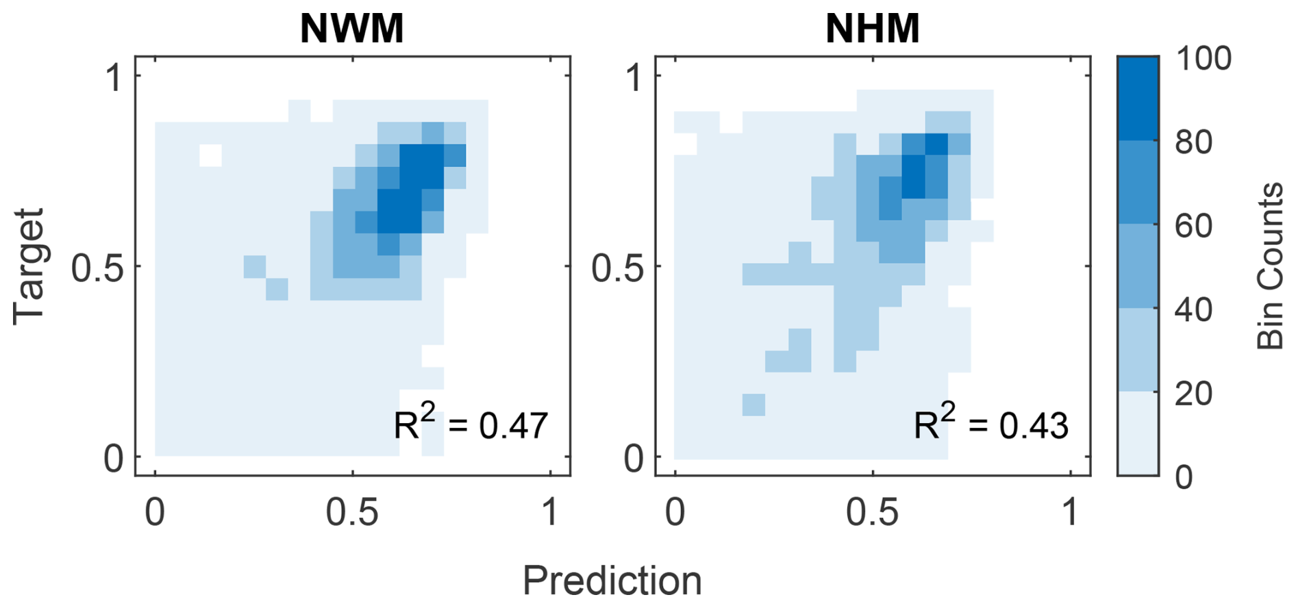
Figure 3 Evaluation of the random forest model prediction of Kling–Gupta efficiency (KGE) at NWM and NHM sites. Results are shown for the out-of-bag (testing) samples. The density scatter plot displays the count of data points in each partitioned bin. For visual clarity, predicted and observed KGE values less than 0 are not plotted, although they are included in the calculation of R² for each model. NWM = National Water Model, NHM = National Hydrologic Model, R² = coefficient of determination.

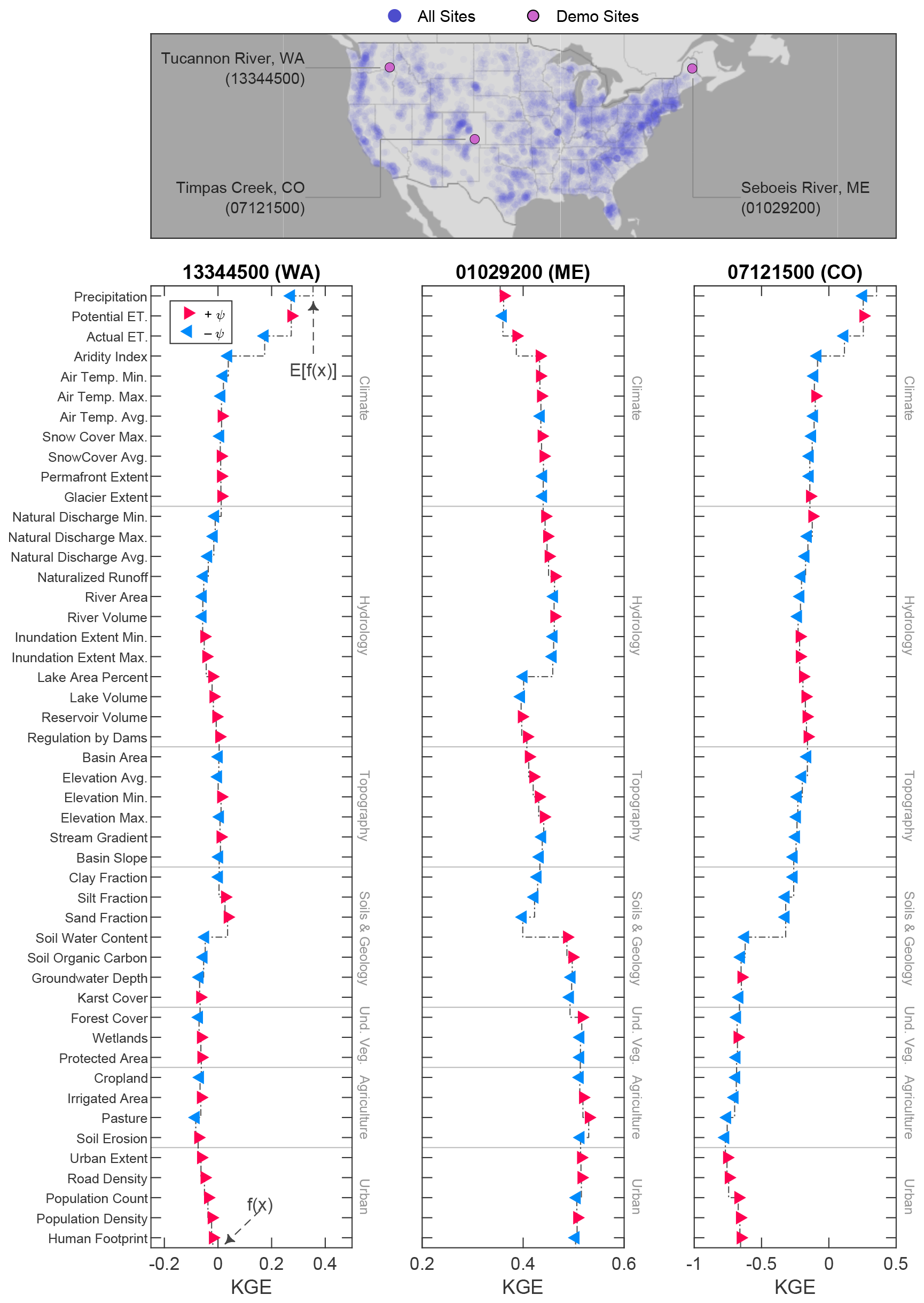
Figure 4 Local structure of Kling–Gupta efficiency (KGE) prediction for the National Water Model (NWM) as illustrated by Shapley value (ψ) waterfall plots at three demonstration sites, indicated by US Geological Survey station numbers associated with stream gauges and two-letter state abbreviations. Each plot begins with the expected value of the model prediction for all sites, E[f(x)], which undergoes marginal alteration (±ψ) by each of the 48 predictor features. The final model prediction, f(x), is equal to E[f(x)] plus the cumulative sum of all marginal contributions. Undeveloped vegetation is abbreviated as Und. Veg.

We investigated the local structure of Shapley values (ψ) at three sites that have been selected to demonstrate various controls on KGE prediction (Fig. 4). We report how the Shapley values explain random forest model predictions of KGE, but it is important to note that these explanations are not necessarily causal but rather reflect correlations identified by the algorithm. The directionality and extent of influence by each predictor are indicated by the magnitude and sign of the predictor's Shapley value (±ψ). Each waterfall plot shows how Shapley values (ψ) of features help to distinguish one site, f(x), from the mean of all sites, E[f(x)]. These three sites were selected to demonstrate various catchment controls, such as climate at Tucannon River, WA; hydrology at Seboeis River, ME; and soils and geology at Timpas Creek, CO. At Tucannon River, the relatively high values of actual evapotranspiration and aridity index at the site cause a decrease (−ψ) in the prediction of KGE at that site. At Seboeis River, the large lake area percentage causes a decrease (−ψ) in KGE prediction, but the high soil water content causes an increase (+ψ) in KGE prediction. At the final site, Timpas Creek, the most influential feature is the low soil water content, which has a considerable negative contribution (−ψ) to KGE prediction. With an understanding of how Shapley values operate at an individual gauge (local scale), we proceed to a global perspective by assessing the aggregate Shapley value results of all 4383 sites.

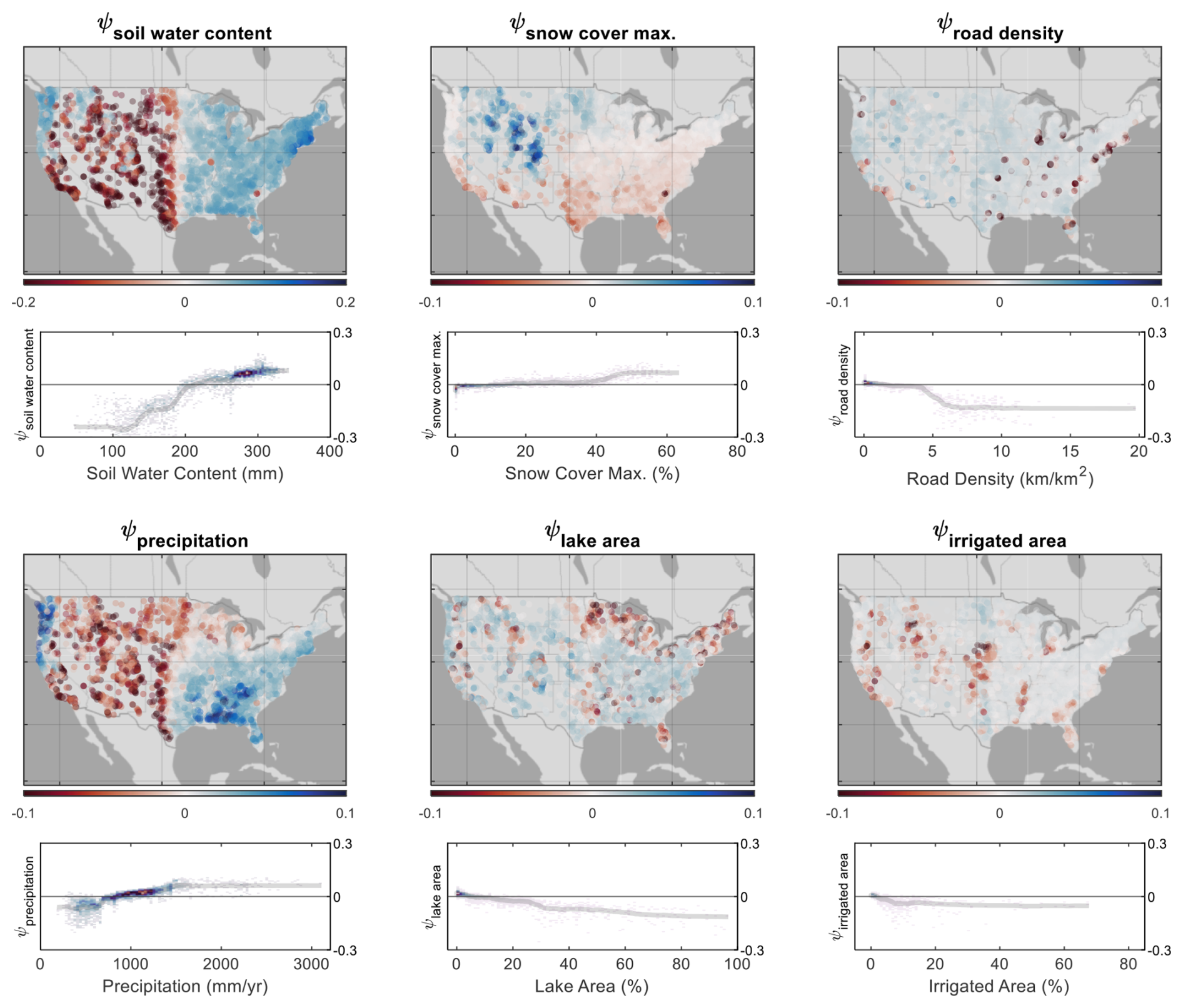
Figure 5 Spatial distribution of Shapley values (ψ) for selected influential features and their impact on Kling–Gupta efficiency (KGE) prediction for the National Water Model (NWM). The color bar represents the magnitude of ψ. The partial dependence plot of each feature is shown. Feature value distributions are represented with a heatmap. A moving average of feature values is indicated by a line to show general trends.

The global structure of Shapley values (ψ) for six important catchment attributes is shown (Fig. 5): soil water content, snow cover maximum, road density, precipitation, lake area, and irrigated area. The marginal contribution of the soil water content variable (ψ_{soil water content}) is positive (+ψ) in areas with high soil water content (east of the 98th meridian and in the Pacific Northwest) and negative (−ψ) in areas with lower soil water content (Great Plains, Intermountain West, and California). The Shapley dependence plot identifies 210 mm soil water content as a threshold from when ψ_{soil water content} increases (+ψ) versus decreases (−ψ) the prediction of KGE. The ψ_{snow cover max.} values are positive in the Rocky Mountains and the upper Midwest. Snow cover maximum has little effect on KGE predictions until a threshold of 40 % is exceeded, at which point maximum snow coverage increases KGE prediction. The ψ_{road density} values are negative in urban centers, when road density exceeds 5 km km⁻², suggesting that high road density decreases the accuracies of model predictions. Otherwise, the presence of roadways has little impact on KGE predictions at lower road densities. A threshold of 900 mm yr⁻¹ in precipitation emerges; precipitation values lower than this threshold lower KGE (−ψ_{precipitation}) and values greater than this threshold increase KGE (+ψ_{precipitation}). The ψ_lake area values are generally close to zero except for when lakes constitute a substantial portion of a watershed (> 10 %), such as in Minnesota and Wisconsin and the northeast region. For ψ_{irrigated area}, watersheds with less than 3 % irrigated area are unaffected by the variable, but beyond a threshold of around 10 %, the presence of irrigation decreases KGE predictions.

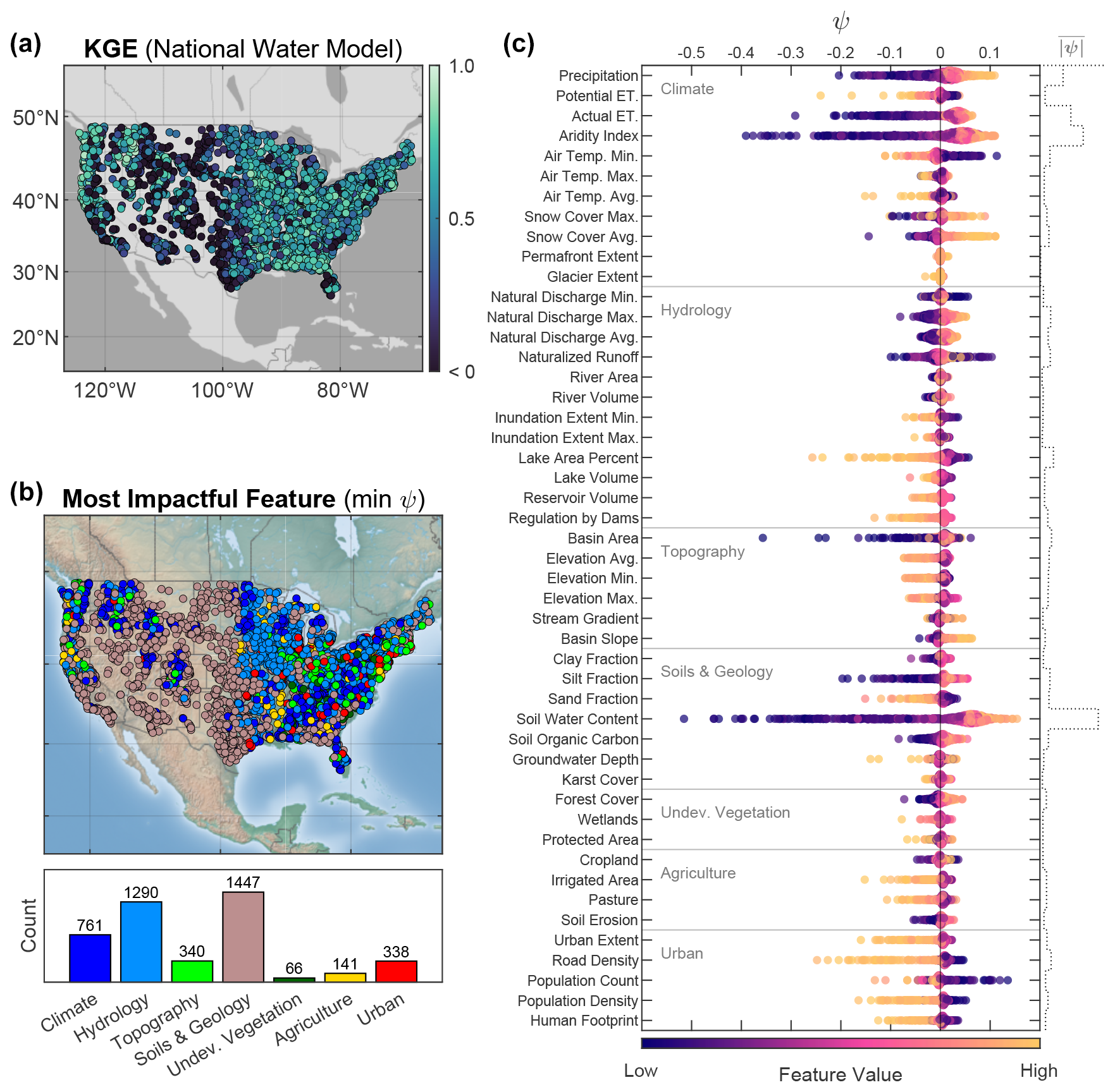
Figure 6 (a) Map of Kling–Gupta efficiency (KGE) for the National Water Model. (b) Map and histogram of the most impactful feature causing poor model performance at each site, i.e., the predictor group having the greatest negative Shapley value (ψ) at a site. (c) Swarm chart of Shapley values for KGE prediction showing feature importance for 48 predictors. The staircase plot on the right axis indicates the mean absolute Shapley value ($\stackrel{\mathrm{‾}}{\left|\mathit{\psi }\right|}$) of all observations for a predictor. The predictor value is the magnitude of the catchment attribute.

Shapley value swarm charts show the directionality and magnitude of feature importance for all 48 predictors (Fig. 6). Globally, the most impactful features (greatest $\stackrel{\mathrm{‾}}{\left|\mathit{\psi }\right|}$) for KGE prediction are ψ_{soil water content}, ψ_{aridity index}, ψ_actual ET, and ψ_{precipitation}. Regarding directionality, higher catchment-scale values of soil water content, aridity index, actual ET, and precipitation increase KGE prediction (+ψ), whereas smaller values decrease KGE prediction (−ψ). Although these are globally the most influential variables, they are not necessarily the most influential at each individual site. We plot the spatial distribution of the most impactful feature group leading to poor KGE scores at each site – that is, the predictor group having the greatest negative Shapley value (min ψ) at a site. The most impactful feature groups at individual sites were climate (n = 761), hydrology (n = 1290), and soils and geology (n = 1447). Soils and geology features, most frequently low soil water contents, reduced KGE most often in the Great Plains and Intermountain West. Hydrology features, typically large values of lake and reservoir storage, reduce modeled KGE in the Midwest. Climate features did not have strong spatial coherence. Next, we assess the distribution of KGE values grouped by most impactful feature (Fig. 7). For the NWM, sites where the most impactful features were soils and geology as well as urban land use had the lowest median KGE values. The results for NHM were similar to NWM except that areas controlled by climate have lower median KGE values for NHM than NWM.

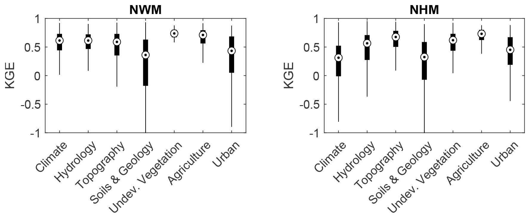
Figure 7 Kling–Gupta efficiency (KGE) performance grouped by the most important variable at each site as identified by Shapley values for the National Water Model (NWM) and National Hydrologic Model (NHM).

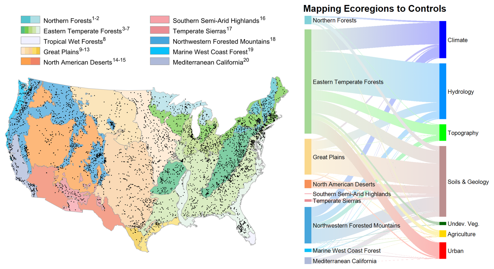
Figure 8 Map of study stream gauges (black markers) and the Ecoregions of North America (as defined in Omernik, 1987). Sankey diagram showing the pairing of ecoregions and impactful feature classes for the National Water Model (NWM) for the Kling–Gupta efficiency (KGE) evaluation metric. Ecoregion classifications are defined using the following superscripts: ¹ Atlantic Highlands, ² Mixed Wood Shield, ³ Ozark, Ouachita–Appalachian Forests, ⁴ Mixed Wood Plains, ⁵ Central US Plains, ⁶ Southeastern US Plains, ⁷ Mississippi Alluvial and Southeast US Coastal Plains, ⁸ Everglades, ⁹ Temperate Prairies, ¹⁰ West-Central Semi-Arid Prairies, ¹¹ South Central Semi-Arid Prairies, ¹² Texas–Louisiana Coastal Plain, ¹³ Tamaulipas–Texas Semi-Arid Plain, ¹⁴ Cold Deserts, ¹⁵ Warm Deserts, ¹⁶ Western Sierra Madre Piedmont, ¹⁷ Upper Gila Mountains, ¹⁸ Western Cordillera, ¹⁹ Marine West Coast Forest, and ²⁰ Mediterranean California.

We map the spatial linkage between ecological regions in the US and the influential features controlling KGE scores at sites contained within these regions (Fig. 8). The ecoregions containing the most stream gauges are Eastern Temperate Forest, Great Plains, Northwestern Forested Mountains, and North American Deserts. Streams in the Eastern Temperate Forest ecoregions are most frequently influenced by, in decreasing order, hydrology, climate, urban, and soils and geology features. For the Great Plains, the most frequent controlling features are soils and geology, followed distantly by hydrology. The Northwestern Forested Mountains are influenced by soils and geology, climate, hydrology, and topography. Lastly, the North American Desert streams are controlled almost exclusively by soils and geology features.

4 Discussion

We investigate the relative importance of catchment attributes for streamflow model performance to diagnose deficiencies in how the hydrologic models represent physical processes. Compared to other parameter-based continental-scale sensitivity analyses (e.g., Mai et al., 2022), our approach provides a post hoc assessment of model sensitivity. That is, perturbing the parameterization of the original modeling framework is not necessary to identify model sensitivities. Rather, sensitivities are deduced (learned) through the identification of the marginal contribution of predictor features to model performance. In this way, our approach identifies how catchment attributes may impact KGE – rather than how model parameters directly impact KGE. The interpretable machine learning approach we present is flexible and model-agnostic, meaning it can be applied to any modeling framework.

4.1 Model diagnostics with interpretable machine learning

The Shapely value approach used in our study is able to make both local (Fig. 4) and global (Fig. 5) inferences from the same model. Shapley dependence plots allow us to infer the individual (marginal) contribution of a feature to the overall model as a function of the feature's magnitude. Compared to traditional sensitivity analyses, which perturb model parameters and observe the resulting impact on a performance evaluation metric (Pianosi et al., 2016), this approach identifies spatial patterns in where models perform well and where they do not and relates that pattern to the spatial variation in catchment attributes. This indirect approach to model sensitivity allows for the identification of attributes that show a high degree of influence on model performance. This approach can serve as an interrogation tool for prioritizing which processes should be better represented within the evaluated hydrologic model structure. Below, we highlight both local and global structures that emerge from our analysis and that allow for the interrogation of NWM and NHM performance.

Local structures emerge whereby a few sensitive attributes can dominate the overall KGE prediction at a site (Fig. 4). This can manifest as a catchment attribute decreasing or increasing prediction accuracies (as measured by KGE) of NWM or NHM. For example, at an arid site on the Tucannon River (WA), the NWM performance is lower at this site than the nationwide average of NWM for all sites because of high actual evapotranspiration and low precipitation conditions. Conversely, at Seboeis River (ME), the higher humidity and soil water content contribute to higher NWM prediction accuracy compared to the nationwide site average. In some instances, multiple competing attributes offset their negative and positive contributions to KGE prediction. At the Seboeis River, the positive contribution to KGE from high soil water content is offset by the negative contribution of a large lake area percentage. Another way to interpret this would be that in the absence of lakes in the basin, the NWM would produce more accurate streamflow predictions at this site – that is, a higher KGE. Therefore, although the model's representation of soil water content at this site increases streamflow prediction accuracy, the simulation of lake water storage (or lack thereof) is inhibiting streamflow prediction. Importantly, the Shapley value approach can also identify features that are not influential for KGE. For example, for all three sites investigated in Fig. 4, the natural vegetation and agricultural variables have a limited influence on KGE. By elucidating the local structure of catchment controls on model performance, this approach allows for inference about which processes are not well-represented by the model. Addressing these processes could be prioritized in further iterations of models to facilitate large increases in model accuracy.

Global structures emerge whereby the Shapley value approach can identify thresholds at which features become influential (Fig. 5). Because our approach considers all sites simultaneously, we can make conclusions about the spatial coherence of influential attributes across regions (Mai et al., 2022). A few variables, most prominently soil water content, are highly influential regardless of whether the variable takes a small or large value. However, some variables have little influence until certain thresholds are crossed (Fig. 5), such as snow cover, road density, irrigation area, and lake area. The ability to resolve threshold behavior in model performance allows for better parameterization of models and identification of areas where increased data collection could improve model calibration (Zehe and Sivapalan, 2009).

This model diagnostic approach provided intuitive results that match the general understanding of streamflow controls across ecoregions (Figs. 6 and S5). The features that commonly decreased model accuracy the most at individual sites (min ψ) were related to soils and geology, hydrology, and climate predictor groups (Fig. 6). The influence of other predictor groups is more variable. For example, urban features (urban extent, road density, population count and density, and human footprint index) are influential in catchments near large metropolitan areas, such Chicago, New York, and Boston, but their influence is largely absent elsewhere. Urban features are the most influential predictors for just 7.7 % of all gauges, but these urban-controlled sites have low KGE values that are similar to sites controlled by the most influential variable group (soils and geology, Fig. 7). In this way, Shapley values show utility in interrogating process-based models by allowing for the identification of overarching controls across all sites in a dataset while not obscuring unique, local controls.

4.2 Natural and anthropogenic drivers of NWM and NHM performance

4.2.1 Climate

Climate processes are of central importance to the goodness of fit for the NWM for many sites (Fig. 6), as indicated by large absolute Shapley values ($\stackrel{\mathrm{‾}}{\left|\mathit{\psi }\right|}$) for climate variables. These results align with results of multiple studies focused on climate processes as drivers for streamflow processes, such as non-perennial streamflow (Hammond et al., 2021; Price et al., 2021; Zipper et al., 2021) and peak streamflow (McMillan et al., 2018). Shapley value results show that climate processes that are related to low water availability (i.e., low values of precipitation, aridity, and ET) decrease the predictive capacity of the NWM (Fig. 5). The inverse is also true, in that streamflow can be simulated more accurately at sites with higher precipitation and lower ET (Fig. 6). Thus, while the NWM is recognized to have poor performance in arid locations (Johnson et al., 2023a), our results show that it is well-suited for prediction in humid locations.

Soil water content, actual ET, and precipitation are the most influential features for determining KGE, all of which are highly seasonal (Elnashar et al., 2021). For example, the spatial map of KGE performance (Fig. 6) is broadly related to precipitation amount and the Shapley value for precipitation (Fig. 5). In areas where climate may have a lower degree of variance throughout the year, NWM accurately simulates streamflow because of the predictability of the hydrologic response in a basin. As an example, we find that the presence of a considerable snow cover (> 40 %; Fig. 5) can improve model predictability; this has been noted elsewhere (Johnson et al., 2023a) and may be related to the predictability of seasonal snowmelt, which can dominate the water balance in cold regions. These results highlight the ability of Shapley values to elucidate the relationships between climate and streamflow and provide important insights into careful parameterization of climate forcings to increase model accuracy.

4.2.2 Hydrology

Of the variables in the hydrology category, we observed the largest effect on KGE in the NWM from lake area and upstream reservoir storage relative to annual flow volume (the degree of regulation), with KGE decreasing as lake area and the degree of regulation increase (Figs. 3 and 4). The modeling of pond and lake storage and release is a known deficiency in large-scale hydrologic modeling, and recent parameterizations have been developed to enhance representation of surface-water depression storage (Costigan and Daniels, 2012; Hay et al., 2018; Hodgkins et al., 2024).

The negative impact of lake and reservoir features on model accuracy is greater on the NHM (Fig. S3) than on the NWM (Fig. 5). As noted earlier, the NHM framework does not simulate any kind of reservoir operations, water withdrawals, or stream releases (Regan et al., 2019). On the other hand, the NWM framework models passive reservoir routing (Cosgrove et al., 2024) to mitigate the confounding effects of lake and reservoir volume on model performance. The Shapley value approach was able to successfully determine that the model without any provision for reservoirs (NHM) is more negatively affected by the presence of reservoirs than the model with routing capability (NWM), underscoring that the method can produce intuitive results that match our conceptual models.

4.2.3 Physiography (topography, soils, and geology)

Hydrologic connectivity controls many facets of the natural flow regime and determines the ability of a watershed to store and release water (Michalek et al., 2023). Parameterizations of soils, geology, and other basin characteristics are highly heterogeneous and mediate many facets of connectivity, many of which are poorly resolved in large-scale hydrologic models (Li et al., 2023). For example, soil water content was the most impactful predictor for KGE according to the Shapley value analysis (Fig. 5), with low values of soil water content greatly impacting the KGE. Accurate simulation of soil moisture patterns, particularly in arid locations, is a well-recognized challenge in the NWM, which can be mitigated by the integration of soil moisture data into the model calibration process (Araki et al., 2025). Other factors that contribute to a high degree of hydrologic connectivity, including a high percent of sand and a low percent of clay (Fig. 6), also highlight the inability of the NWM to resolve storage dynamics, which likely results from inadequate parameterization of areas that have highly seasonal soil water content (Hughes et al., 2024) and the inability of the current generation of NWM to represent losing streams (Jachens et al., 2021; Lahmers et al., 2021).

We also identified predictor variables commonly associated with the physiography of headwater systems as important predictors of KGE (Fig. 6), such as drainage area and mean elevation. Headwater systems are defined as “surface-water catchment areas and groundwater zones that contribute water, material, and energy to a headwater stream” (Brinkerhoff et al., 2024; Golden et al., 2025). Headwater streams typically have smaller drainage areas and higher mean elevations, which our approach found were associated with lower KGE values for NWM predictions, possibly because NWM simulates atmospheric states and fluxes on a 1 × 1 km² grid cell and can misrepresent processes that are on the scale of headwater systems. These headwater systems are low-order and highly variable in their flow regimes (Rojas et al., 2020), both of which are inadequately represented in NWM.

4.2.4 Anthropogenic processes

Of the variables related to anthropogenic influence, we note that urban features, such as urban extent, road density, population count, population density, and human footprint, typically decrease KGE values for modeled streamflows (Figs. 5 and S4). The construction of urban drainage networks has been recognized to increase the connectivity of water, solutes, and sediment and to add additional pathways of transport through the artificial routing of water (Zarnaghsh and Husic, 2021). In a continental-scale analysis of the NWM, urban areas exhibited some of the largest bias (Johnson et al., 2023a), in part due to the presence of constructed drainage networks. Notwithstanding this limitation, the NWM has shown some success in simulating hydrology when artificial urban channels, which differ from natural flow paths, are manually delineated within the flow grid (Pasquier et al., 2022). However, manual delineation is not feasible for applications intended for regional or continental scales, such as NWM and NHM.

Our model identifies a threshold of around 5 km km⁻² for roadways as the initiation point whereby the presence of roadways decreases the accuracies of NWM and NHM predictions (Figs. 4 and S3). The sensitivity of the roadway density feature may indicate other associated infrastructure, the configuration of proximal impervious areas, and the relative amount of human alternation of surface flow generation and routing mechanisms not picked up by considering imperious area alone. Population and population density similarly likely indicate associated infrastructure that alters the flow timing and magnitude of water delivery to rivers (Hopkins et al., 2019). For example, leaky infrastructure can result in elevated low flows beyond natural background levels (Bhaskar et al., 2020). Regarding agriculture, irrigation return flows have been shown to be important to flow generation processes, particularly in lower-elevation, arid rivers (Putman et al., 2024). These urban and agricultural features can decrease model accuracy when present, but the absence of these features does not necessarily increase model accuracy (Fig. 6).

4.3 Limitations and future research

Our interpretable modeling approach has provided several insights into interrogating process deficiencies in the NWM and NHM. Although the inferences we derived from the Shapley values are robust, interpretable, and intuitive, the analysis approach itself is not causative (Lundberg et al., 2020). Thus, some inferences may occur due to indirect correlation (Heskes et al., 2020). We took precautions to mitigate the effect of feature correlations while constructing the random forest model, such as random exclusion of features during tree construction and out-of-bag sampling (Fox et al., 2017). Our approach provides confidence because, as we noted earlier, many of the inferences we derived with the Shapley values match the causative and mechanistic model assessments performed by others (Hodgkins et al., 2024; Hughes et al., 2024; Jachens et al., 2021; Pasquier et al., 2022).

The interpretable modeling approach has its own set of limitations. First, predictions made by Shapley values are a function of (1) the set of sites considered, in this case 4383 stream gauges in the United States used in NWM and NHM assessment, and (2) the choice and performance of the predictive model, which in this case was a reasonably accurate random forest model (R² ≥ 0.43). With regard to the first point, if our analysis approach were applied to interpreting the KGE values for streamflow predictions made by applying the Soil Water and Assessment Tool (SWAT) to Europe (Abbaspour et al., 2015), the order and magnitude of influence by various features would undoubtedly change. To the second point, although our random forest model is reasonably accurate, it only explains 47 % of the variance in KGE prediction for the NWM (and 43 % for the NHM). While our model effectively captures dominant global trends and local structures, it still leaves more than half of the variance in KGE predictions unexplained. Future studies could explore ways to further explain this variance. Additionally, we consider only the KGE goodness-of-fit metric in this study, but if we were to interpret other goodness-of-fit metrics, such as the Nash–Sutcliffe efficiency, there is potential that inferred controls on model performance may change. This is because all goodness-of-fit metrics encode for – and are biased by – various information contained within streamflow time series (Clark et al., 2021). Nonetheless, of the common evaluation metrics presently applied in the hydrologic literature, use of the KGE is increasing because of its lower overall bias and provision for balanced results during low- and high-flow conditions (Althoff and Rodrigues, 2021).

Several opportunities exist for overcoming limitations and making improvements to the data inputs and model outputs. First, the spatial extent and resolution of the catchment attribute dataset may be too coarse, particularly for smaller basins. Of the 48 catchment attributes derived from the BasinATLAS dataset (Linke et al., 2019), spatial resolutions range from 3 arcsec for elevation to 5 arcmin for land use. At 40° N, the median latitude of the CONUS, these arc values correspond to ∼ 85 m and ∼ 7 km, respectively. These datasets were aggregated to 15 arcsec (∼ 350 m), and thus the calculated attributes for smaller basins are more uncertain due to a smaller sample size of attribute estimates contained within basin bounds. A second data limitation is that the catchment attribute dataset represents a snapshot-in-time value for all basins (Linke et al., 2019). However, catchments and their characteristics, particularly land use, may change substantially over time. The hydrologic models are simulated over multiple decades (1984 to 2016), during which change may occur and be captured within the process-based representation of the models but not in the catchment attribute dataset. Improved spatial resolution and temporal evolution of catchment attributes could provide deeper insights into identifying NWM and NHM process deficiencies. There is potential that latent factors not explicitly included as attributes in BasinATLAS, such as wastewater effluent or groundwater pumping, exert control on NWM and NHM performance. Finally, the process-based models used here vary in their spatial and physical representation of hydrologic processes. Process-based model differences in routing schema, spatial groupings (hydrologic response unit vs. grid-based), and subsurface properties could result in local differences in model performance. While these specific model structural variations are less likely to dominate the explanation of broad, CONUS-scale patterns identified in our analysis, they can contribute to residual unexplained variance.

Looking forward, the National Oceanic and Atmospheric Administration (NOAA), the developers of NWM, are expanding modeling capacity with their Next Generation Water Resources Modeling Framework (NextGen; Ogden et al., 2021). In addition to a uniformly applied national hydrologic model, there will be tools for identifying the best model/parameterization for each individual location and then modeling regions as patchworks of individual/local models (Cosgrove et al., 2024). In addition to assessing overall flow performance, this approach could be used for specific components of the flow regime, such as high and low flows. For example, studies that have focused on individual components of non-perennial drying regimes have used a random forest approach coupled with partial dependency analysis (e.g., Price et al., 2021). The Shapley value approach used in this study could be used in a similar way to evaluate magnitude and directionality of impact between predictor values and flow regimes across systems. Further, modules are planned for purely data-driven approaches, like long short-term memory models (Frame et al., 2021, 2025). Our interpretable modeling approach provides a starting point to inform the parameterization of local-scale and regional-scale applications in the next generation of hydrologic models.

5 Conclusions

The interpretable machine learning technique we present is flexible and model-agnostic. We use the technique to identify potential process-based deficiencies in two continental-scale hydrologic models: the National Water Model and the National Hydrologic Model. Compared to other parameter-based continental-scale sensitivity analyses, our approach provides a post hoc assessment of model sensitivity. This method allows for the identification of thresholds after which a feature begins to negatively impact streamflow model performance. Globally, soil water content was the most common feature influencing the accuracies of streamflow simulations, followed by aridity, evapotranspiration, and precipitation. We interpret the results to indicate that the present formulations of NWM and NHM have limited ability to resolve soil water storage and release, particularly in arid locations. Locally, the presence of lakes and reservoirs was related to decreased model accuracy as was the presence of roadways and irrigation canals. Our results suggest that further refining how these influential processes are represented in large-scale hydrological models would result in the largest increases in model accuracies. This study demonstrates the utility of interrogating process-based models using data-driven techniques and interpretable machine learning, which has broad applicability and potential for improving simulation of large-scale hydrology and water quality.