Technical note: Image processing for continuous river turbidity monitoring – full-scale tests and potential applications

The development of continuous river turbidity monitoring systems is essential since this is a critical water quality metric linked to the presence of organic and inorganic suspended matter. Current monitoring practices are mainly limited by low spatial and temporal resolutions and costs. This results in the huge challenge of providing extensive and timely water quality monitoring at the global scale. In this work, we propose an image analysis procedure for river turbidity assessment using different camera systems (i.e. fixed-trap camera, camera on board an uncrewed aerial vehicle and a multispectral camera). We explored multiple types of camera installation setups during a river turbidity event artificially re-created on site. The outcomes prove that processed digital-camera data can properly represent the turbidity trends. Specifically, the experimental activities revealed that single-band values were the most reliable proxy for turbidity monitoring in the short term, more so than band ratios and indexes. The best camera positioning, orientation and lens sensitivity, as well as daily and seasonal changes in lightning and river flow conditions, may affect the accuracy of the results. The reliability of this application will be tested under different hydrological and environmental conditions during our next field experiments. The final goal of the work is the implementation of this camera system to support existing techniques and to help in finding innovative solutions to water resource monitoring.

1 Introduction

Nowadays, compliance with the European Water Framework Directive and World Health Organization (WHO) guidelines for water quality is becoming more and more challenging (Santos et al., 2021; WHO chronicle, 2011) since human-related activities and climate change are heavily impacting water resources. Therefore, freshwater will be a more and more valuable resource which deserves to be properly monitored, exploiting all available techniques, and also wisely managed (Manfreda et al., 2024). In this context, turbidity is a key factor for water quality monitoring and an optical property often used as an indicator of suspended particles and floating pollutants (Stutter et al., 2017; Tomperi et al., 2022). In inland waterbodies, turbidity level and trophic state can strongly change with seasonality (Jalón-Rojas et al.,2015), soil erosion, extreme events and farming activities (Lu et al., 2023). Despite expensive costs for instruments and personnel, conventional in situ monitoring techniques, using regular but not frequent sampling, return information too poor to properly characterise the temporal trends and spatial variability of hydrological and environmental conditions in river basins (Guo et al.,2020), usually underestimating the real loads (Gippel,1995).

In the last few years, several innovations have been introduced into hydrological monitoring which exploit satellites, uncrewed aerial vehicles (UAVs) or fixed camera systems in combination with image-processing and machine learning techniques (Manfreda et al., 2018; Manfreda and Ben Dor, 2023). These methods offer the opportunity to provide large-scale and detailed information on specific hydrological processes with relatively low costs. Within this context, many remote sensing applications for water quality applications have been developed (Ritchie et al., 2003; Ahmed et al., 2020), exploring the potential information coming from the water spectral signatures (Gholizadeh et al., 2016) and investigating the dynamics of riverine ecosystems (Zhao et al., 2019; Lama et al., 2021).

Many of these studies developed turbidity estimation algorithms using satellite products, mainly for very large rivers, reservoirs (Potes et al., 2012; Constantin et al., 2016; Garg et al., 2020; Hossain et al., 2021) and coastal areas (Dogliotti et al., 2015). Unfortunately, satellite spatial resolution cannot provide distributed estimations of water turbidity (WT) along the entire river network (Sagan et al., 2020), and the frequency of data collection is limited by the satellite revisit period, usually 5–10 d for Sentinel-2 and Landsat 8 (Jia et al., 2024). Recent studies are starting to investigate the perspective of using digital cameras and low-cost optical sensors for river turbidity monitoring (Gao et al., 2022; Droujko and Molnar, 2022). However, no studies have focused on the potential of image analysis applied in a real riverine environment yet. Such an application could definitively grant continuous high-frequency data across inland waterbodies even without spatial resolution issues. Moreover, latest advances in computer vision techniques can certainly help us in extracting water quality information from images. The present study explores the use of an image-based monitoring procedure for river turbidity estimation. It was carried out within a real river where an artificial perturbation of the water turbidity has been used to find the optimal configuration for camera systems, the best-performing band and the range of applicability of the procedure. This paper contains a short introduction, along with the background used; the field experiment and methods are illustrated in Sect. 2, and, finally, the results are discussed, providing our final remarks.

1.1 RGB image acquisition and interpretation

The use of digital cameras in river monitoring activities can increase our knowledge of the real status of waterbodies, solving the above-mentioned cost and data resolution problems of the existing techniques. The challenge of image-based procedures is the proper red, green and blue (RGB) signal interpretation and processing. Goddijn-Murphy et al. (2009) affirm that cameras can be seen as three-band radiometers, able to measure the water-leaving spectral response. The actual water upwelling light R_w that reaches the camera lens, schematically shown in Fig. 1, is the sum of various reflectance components of the suspended particles (R_s), the riverbed background (R_b) and the water itself. One component could prevail over the others, depending on the variability of hydrological (water level, flow velocity, etc.) and environmental (suspended-solid concentration, floating pollutants, etc.) characteristics of the river. Digital cameras receive these inputs and return a signal in terms of RGB pixel intensity values.

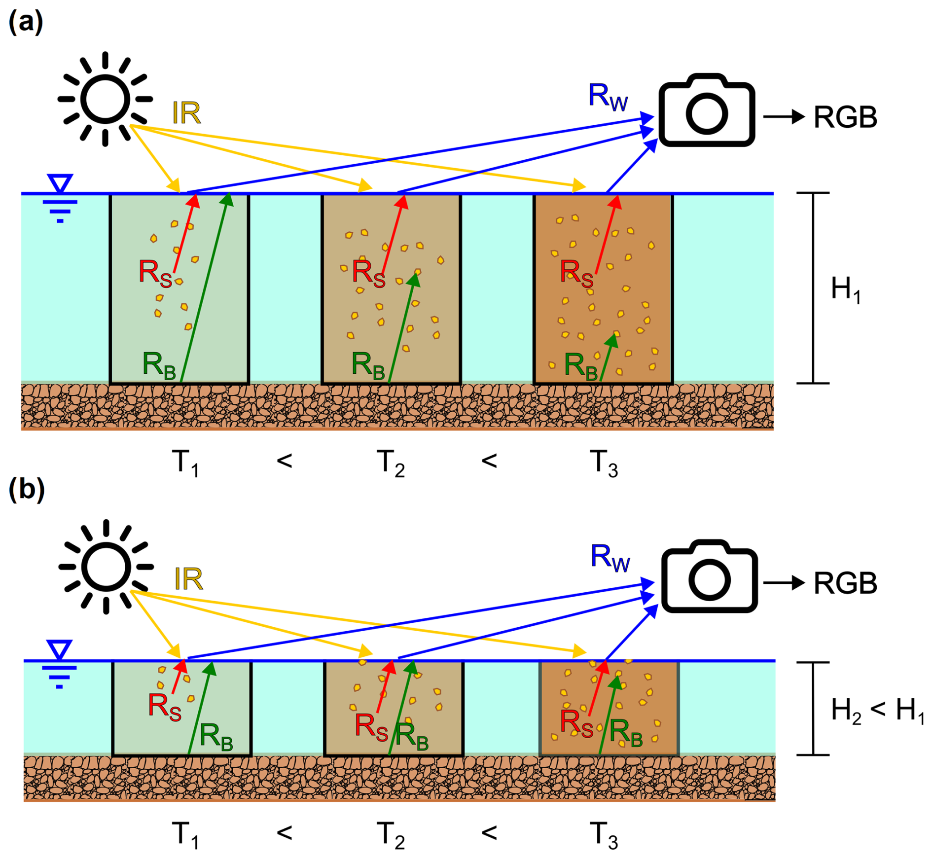
Figure 1 Light behaviour within shallow (b) and non-shallow water (a): the solar irradiance (IR) passes through the water, whose reflectance (R_w) is influenced by the background (R_b) and suspended-particle (R_s) presence, by varying the water level (H). Finally, the total water reflectance (R_w) signal is caught by the digital camera that produces an image with different pixel intensities of red, green and blue values (RGB).

1.2 Turbidity image-based measurements

In the literature, there is a robust relationship between digital-camera output and water quality indicators. Each of these methods requires specific solutions to provide trustable results based on the absolute water colour estimation under changing light conditions. For instance, Goddijn and White (2006) fixed a pipe around the camera lens to avoid external reflections for adjusting the image data collection. Leeuw and Boss (2018) developed an innovative smartphone app called “Hydrocolor” using images of the sky and a grey card near the camera's view field as radiometric references for turbidity estimation from the pictures of the water. Nevertheless, the reliability of their results strongly depends on the quality of the unsupervised image data coming from the citizens and the environmental conditions, resulting in inaccurate estimates for water surface roughness and changing weather conditions. More recently, Ghorbani et al. (2020) provided a continuous monitoring camera tool for suspended-sediment concentrations (SSCs) and turbidity by using image analytic methods and machine learning techniques. They found evidence of a correlation between SSCs and camera images in their experiments under laboratory-controlled conditions.

In real riverine environments, there are many more variables to consider. The image reflectance can be strongly influenced by several factors regarding river flow and light condition variability. Moreover, different bands could provide several information about the water status considering both single bands and their combinations. Nechad et al. (2010) demonstrated that single bands in the red and NIR (near-infrared) spectral ranges give a robust outcome in mapping total suspended matter in coastal turbid waters using several satellite data sources. However, the choice of single bands or their combination is dictated by the concentration of the suspended solids and the type of floating pollutants, as well as the water depth and riverbed background. In addition, the accuracy of the estimates is certainly influenced by the camera positioning and orientation with respect to the examined river section.

1.3 River turbidity monitoring field campaigns

In Fig. 2, the preliminary results of our long-term monitoring data of 2022 are shown. We conducted a field experiment directly on the river. The installation setup was very simple: only one trap camera installed beside the river, a radiometric calibration panel installed on the other side and turbidimeter measurements, as described in detail by Miglino et al. (2022).

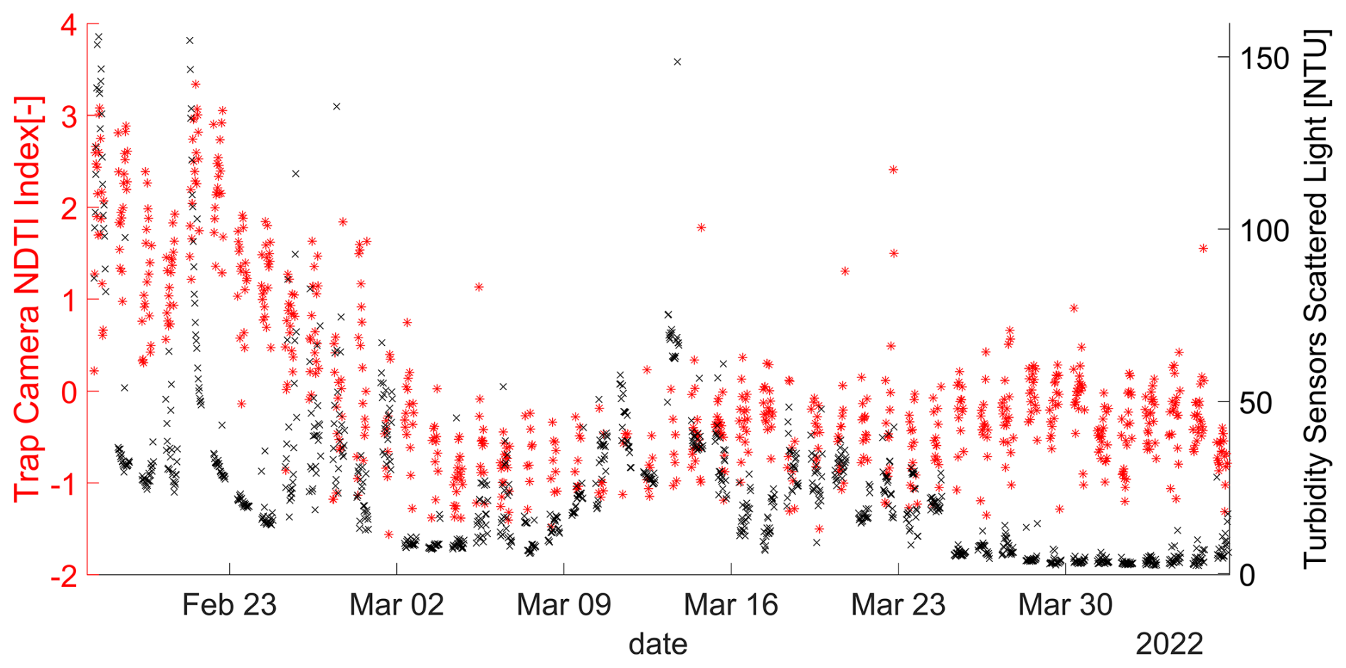
Figure 2 Comparison of turbidimeter measurements (“×” symbols in black) and trap camera NDTI index (“*” symbols in red) during long-term monitoring from February to April 2022.

The trap camera data were compared with the sensor measures. The data collected during the night and under poor light conditions were not considered. We selected from the literature (Lacaux et al., 2007) the normalised difference turbidity index (NDTI) derived from RGB imagery as the most representative index for the camera results. Image data were also standardised by hour of the day to account for long-term variability in sunlight conditions, ensuring comparability across months.

We can already observe a clear correspondence between the variables, especially for the two main turbidity events of February 2022, but also conflicting results for the other low–moderate turbidity peaks.

This first field experience provided us the knowledge needed to design a proper experimental setup in the further studies. In light of these results, we felt the need to investigate the factors influencing the monitored process by designing the short-term experiment of February 2023, proposed in this work.

Our analysis involved the installation of a trap camera (TC), a multispectral camera (MSC) and an uncrewed aerial vehicle (UAV) in order to examine the best spectral response of red, blue, green and NIR bands and their combinations, as well as the best camera installation setup.

The purpose of the field campaigns was to conduct tests on the potential practical applications of the image processing for river turbidity monitoring. This tool can promote the development of early-warning networks at the river basin scale, moving water research forward thanks to a large increase in the data on waterbodies and a reduction in operating expenses.

2 Materials and methods

2.1 Full-scale experiment

The field experiment took place in February 2023 at the monitoring station of Meisdorf, Germany, better described in Miglino et al. (2022). The selected river section was the Selke River, within the TERENO (TERrestrial ENvironmental Observatories) global change exploratory catchment managed by the Helmholtz Association, Germany (Wollschläger et al., 2017). Recently, the Bode basin has gone through prolonged droughts, from 2015 to 2019, resulting in changes in land use and water quantity and quality. This could potentially also impact the suspended-solid load and the pollutant concentration. In this experiment, a synthetic turbidity event was recreated by adding kaolin clay into the water, upstream enough from the monitored river cross-section to ensure the complete mixing of the tracer (Fig. 3). Kaolin is usually exploited to prepare turbidity standard solutions. In addition, it is a harmless, easy-to-handle and cheap mineral, which is also a common silicate in natural soils and sediments.

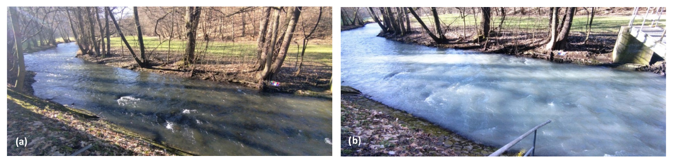
Figure 3 View of the Selke River before (a) and during (b) the synthetic turbidity peak in the field experiment.

We conducted the tracer experiment on 14 February 2023, adding 50 kg of kaolin tracer, evenly distributed, to the whole stream cross-section 700 m upstream from the monitored river section at 12:05 local time (UTC+01:00). The mean flow velocity was 0.47 m s⁻¹, the flow discharge was 2.3 m³ s⁻¹, the water level was 0.54 m, and the width of the river section was 9 m. The turbidity level started to artificially increase after 12:20, the peak was reached around 12:30, and the event ended after 13:00.

Several monitoring instruments were used during the experiment: three low-cost trap cameras (TCs, Ceyomur CY50), one multispectral camera (MSC, Tetracam ADC Snap) and one uncrewed aerial vehicle (UAV, DJI Mavic 2 Enterprise Dual); these were placed in different positions. By looking at Fig. 4, the MSC, in red, was installed on the bridge, and the square in red represents its field of view. Two TCs were installed on the left riverbank (LRB) and the right riverbank (RRB), while the third TC was fixed on the bridge. The last camera was on the UAV, which ensured a zenithal field of view on the river section, indicated by the light-blue square. The flight height of the UAV was 5 m.

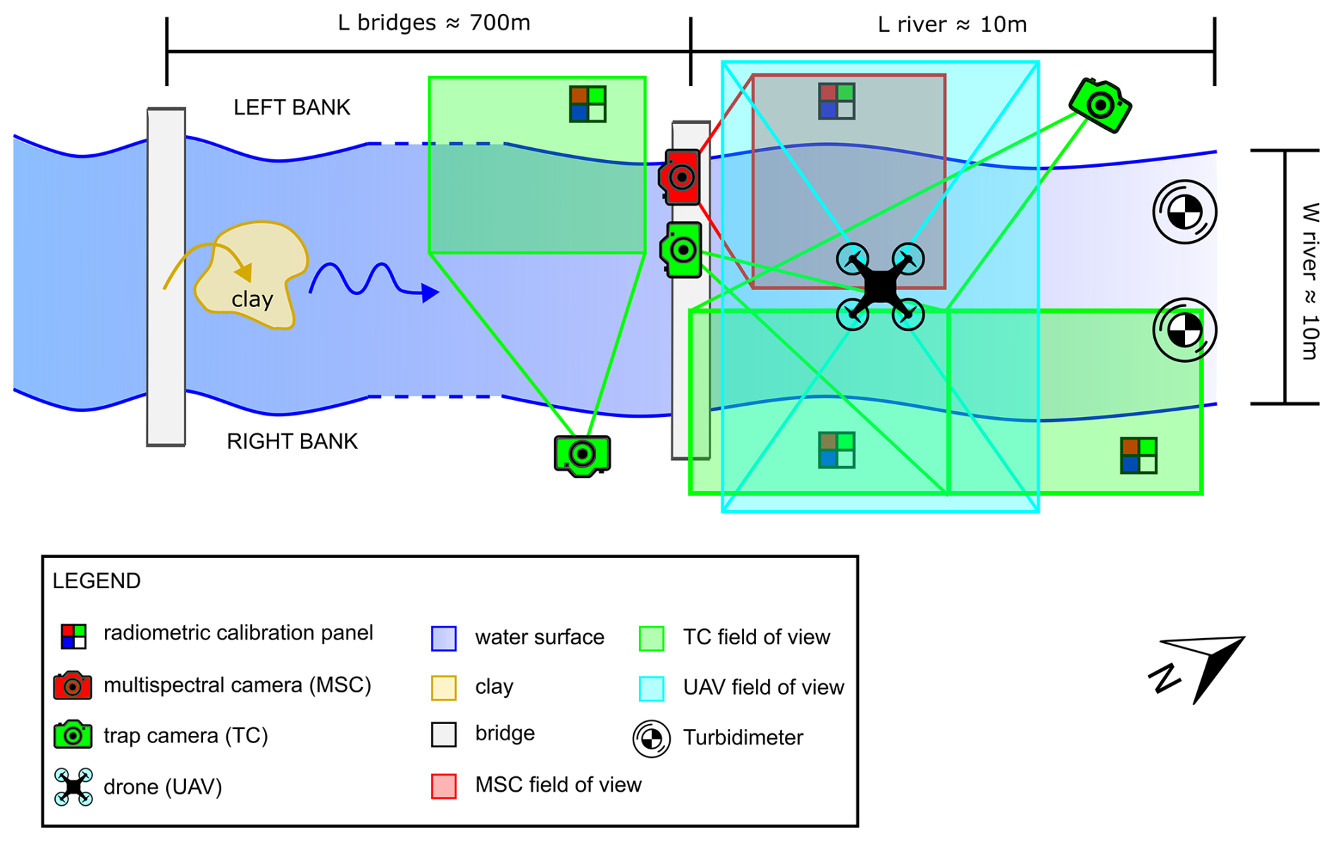
Figure 4 Plan of the monitored river section during the field experiment, showing the generated synthetic turbidity events, using a kaolin clay tracer.

The collected data could be affected by sunglint, shadows and other external light sources. For these reasons, it is essential to find the optimum camera installation design for minimising the uncertainties from water images. The camera data were compared to the measurements of the turbidimeters installed underwater in the river cross-section (Fig. 5). They were located at a distance of 2 m from the right and from the left stream bank for ensuring the detection of the complete mixing of the suspended solids.

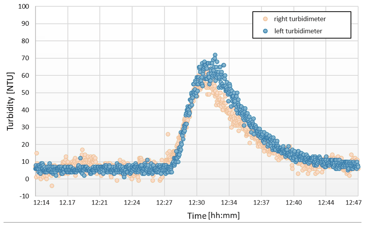
Figure 5 Optical measurements of turbidity using two turbidimeters installed on the right and the left riverbed sides during the experiment. The colour schemes used in this figure are accessible to persons with colour vision deficiencies.

The frame set in Fig. 6 displays all of the camera's fields of view along the stream during the experiment. The region of interest (ROI) was selected, making sure that it included only the water surface area. The mean of the pixel values inside the ROI was considered to be the representative value for the turbidity level for each single picture. Moreover, a radiometric calibration panel (RCP) was installed within the picture area, close to the investigated water surface. This consisted of a waterproof plastic laminated panel containing the reference RGB colour values for the image-processing steps below.

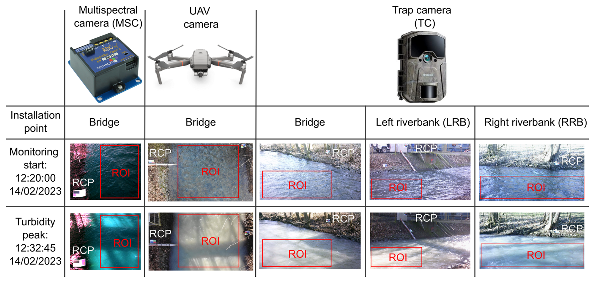
Figure 6 Frame set of the camera types, fields of view and installation points at the start and peak event time of the field experiment.

2.2 Image-processing procedure

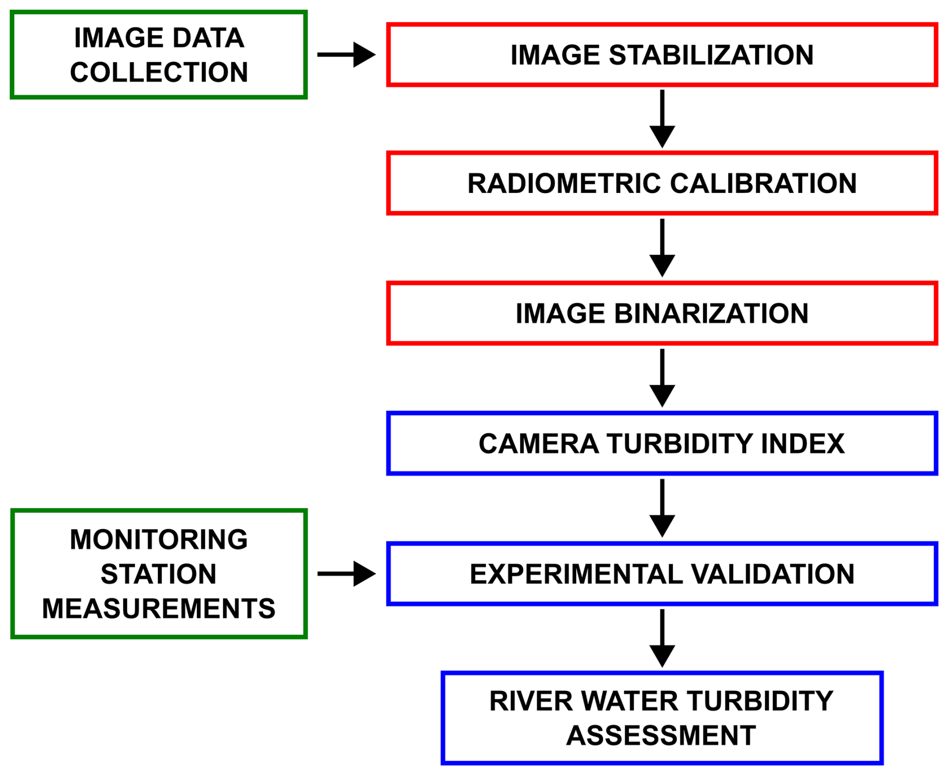
This work defines and tests an image-based method that takes into account variables occurring within time- and site-specific riverine environments. It is important to build a robust procedure since the acquired camera data cannot provide information as they are because they are not yet comparable to physically meaningful units. Herein, our workflow (Fig. 7) sets out the general algorithm of image processing for WT analysis, starting from a correct image extraction and stabilisation. Then, the steps of radiometric calibration and binarisation allowed us to homogenise and select the relevant features from the image data. Finally, the WT indexes were defined from processed signals and validated by field measurements to train the model and to quantify the river turbidity level.

Figure 7 Image-processing procedure.

2.2.1 Image extraction and stabilisation

The image data were stored as time lapses with a set frame rate depending on the type of camera. The number and the format of the extracted images were fixed for each time lapse frame – also collecting frequencies – to ensure the correct comparison between cameras and measurement data.

The image sequences were involved in the image stabilisation process because the position of the objects in the scene could be shifted by environmental factors and camera instability. The image stabilisation techniques performed an automatic detection and matching of features within the selected image area close to the RCP (Fig. 8). In particular, we used the Harris–Stephens corner detection algorithm to identify feature points and to remove apparent movements and jitter within the field of view in the videos (Harris and Stephens, 1988; Abdullah et al., 2012). This step was necessary to grant the correct detection of the RCP and ROI location required for the following image analysis processes.

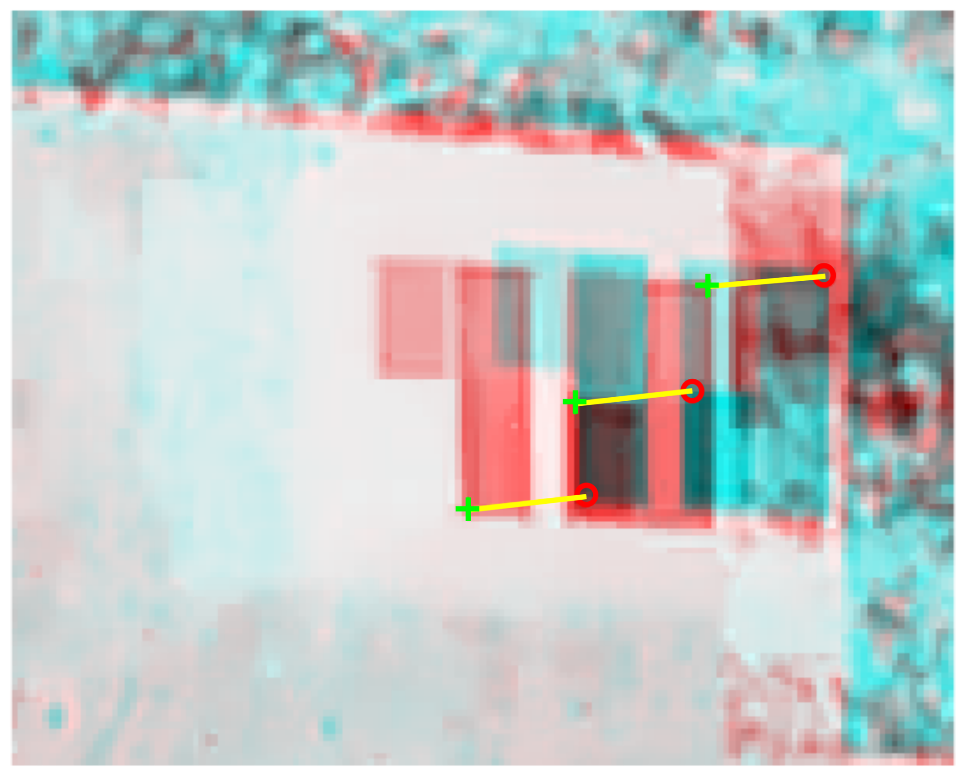
Figure 8 Stabilisation of the RCP coordinates for each extracted frame. The yellow lines show the panel shift during a camera monitoring period of 2 months.

2.2.2 Radiometric calibration

For absolute radiometric correction in monitoring activities where the distance between the ground and the camera is less than 100 m, it is assumed that the atmosphere does not influence the light signal. Nevertheless, other site-specific and meteorological variables can still affect the camera measurement (Daniels et al., 2023). The radiometric signal of an object is influenced by the geometry of the measurements, depending on the relative positions of the sun, the measured object and the optical sensor. The direct–diffuse ratio, the atmosphere absorption and scattering of the solar radiation in the space from the object to the sensor, as well as the camera sensitivity, are all significant factors influencing the natural illumination conditions. Using reference targets or recognised radiometric standards within the scene is necessary to convert the uncalibrated image pixel intensity (PI) values, also called digital numbers (DNs), into radiometrically meaningful units such as reflectance or radiance (Guo et al., 2019; Kinch et al., 2020). In this experiment, we chose a simplified design of the radiometric calibration panel, with the assumed reference values (RV_rc) of the maximum PIs of red, green and blue for all of the images (Fig. 9b) being considered to be the mean of the respective single-band values of the pixels inside the panel squares.

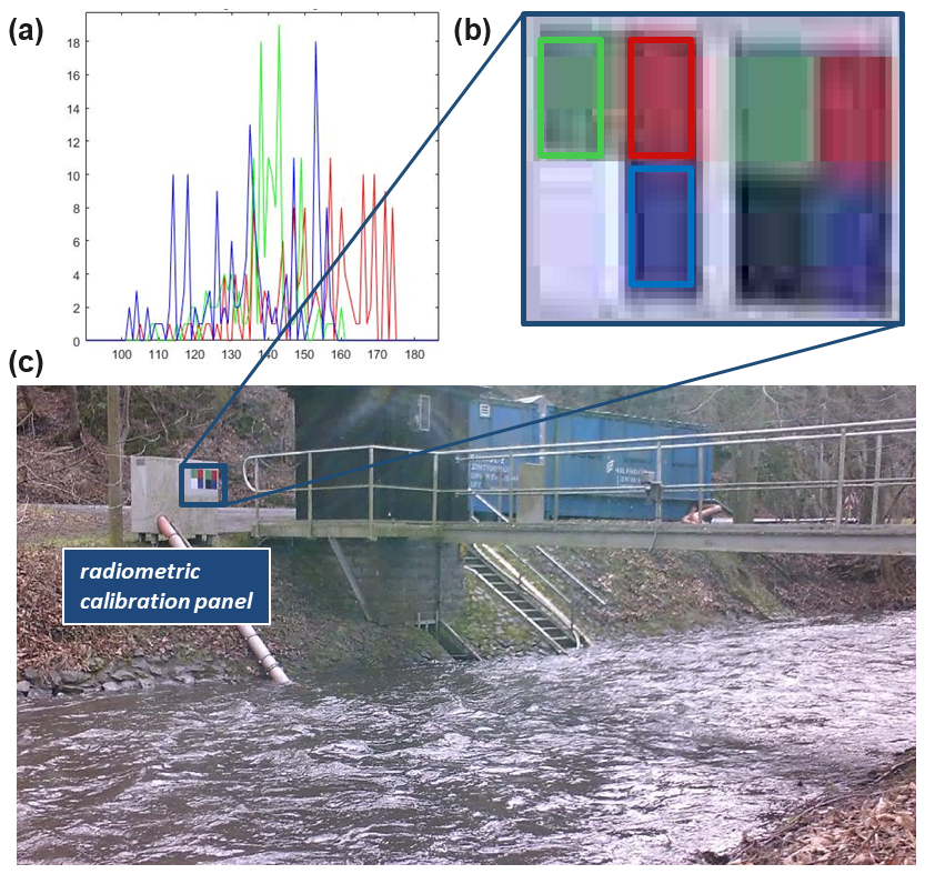
Figure 9 Example of radiometric calibration procedure applied to a TC image using the reference mean RGB values (a) of the radiometric calibration panel (b) installed within the camera field of view (c).

The image PI values were reassigned considering the RCP reference values frame by frame, for each band, as follows:

$$\begin{array}{}\text{(1)}& \text{PIrc}=\mathit{\{}\mathrm{1},\text{PI}/{\text{RV}}_{\text{rc}}\mathit{\}},\end{array}$$

where RV_rc is the panel reference value of red, green and blue for the radiometric calibration process.

PI value ranges for each band go from 0 to 255, but we considered normalised values between 0 and 1. Once the radiometric signal is correctly calibrated, the effect of changes in light conditions on the image information is substantially reduced. Therefore, some image areas could still be affected by sun glare and overly intense shadow. These pixels must be removed by binarisation because they do not contain useful information about the water reflectance.

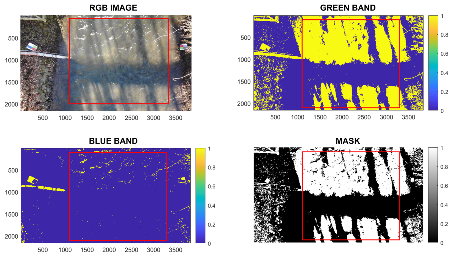
2.2.3 Image binarisation

Image binarisation techniques convert images into binary representations, typically applying predetermined thresholds to grey-scale or RGB values. Here, the adopted procedure follows Otsu's approach (Otsu, 1975). The global threshold was defined separately for each band and for each frame as a result of the minimisation of the weighted variance of two clusters. All of the values above this threshold are replaced with 1, while the other values are replaced with 0. The procedure involves iterations through every image pixel and counts the occurrence of each intensity. In this way, only the actual water reflectance information can be retrieved from the pictures.

In more detail, looking at Fig. 10, we obtained a perfect binary masking from the starting RGB image. Thanks to the right combination of the binarised bands, we managed to remove the pixels with signal distortions due to the effect of sun glare; shadows; and also external objects such as the branches that fall inside the camera ROI, bordered by the red line in the figure. Moreover, this step of the procedure highlights the importance of the information contained in each band. For example, the blue band is not effective in turbidity estimation, but it allows us to isolate and remove critical parts of the image.

Figure 10 UAV image masking with binarisation procedure.

2.2.4 Water turbidity camera index

All the information coming from the camera bands could be properly considered for getting information on WT level in the monitored river site. We selected the most representative remote sensing applications for each band and index, as explained in Table 1.

Table 1 Camera band combinations selected for on-site river turbidity remote measurements.

Single green and red bands were considered to be the most representative signals for identifying the turbidity. The NIR band is also effective in detecting very high turbidity levels. Some ratios between these bands were taken into account too. We selected from the literature the ratio between red and green, the normalised difference turbidity index (NDTI) derived from RGB imagery, and the normalised difference water index (NDWI) that combines NIR and green bands.

3 Results

Our experiments highlighted the capability of digital cameras to detect variations in WT level. We observed that digital-camera results are influenced by several factors, such as the type of sensor adopted and the camera sensitivity, position and orientation. In particular, the MSC results in Fig. 11 describe distinct behaviours of the single bands. Red and green bands can capture turbidity increases above the measured value of 20 NTU, while the NIR-band spectral response is much lower. Since the NIR band is totally absorbed by the water surface, its substantial changes can be detected only for very high concentrations of suspended particles. If we consider the NDWI, the correlation between the camera and turbidimeter data becomes more consistent; this is also the case for red and green bands.

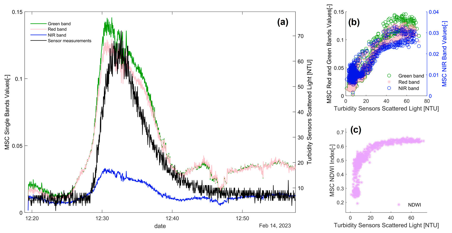
Figure 11 (a) Comparison between turbidimeter measurements and data from the multispectral camera (MSC) installed on the bridge. (b) Scatterplot of the MSC single-band values and on-site measurements; (c) scatterplot of the MSC NDWI values and on-site measurements. The colour schemes used in this figure are accessible to persons with colour vision deficiencies.

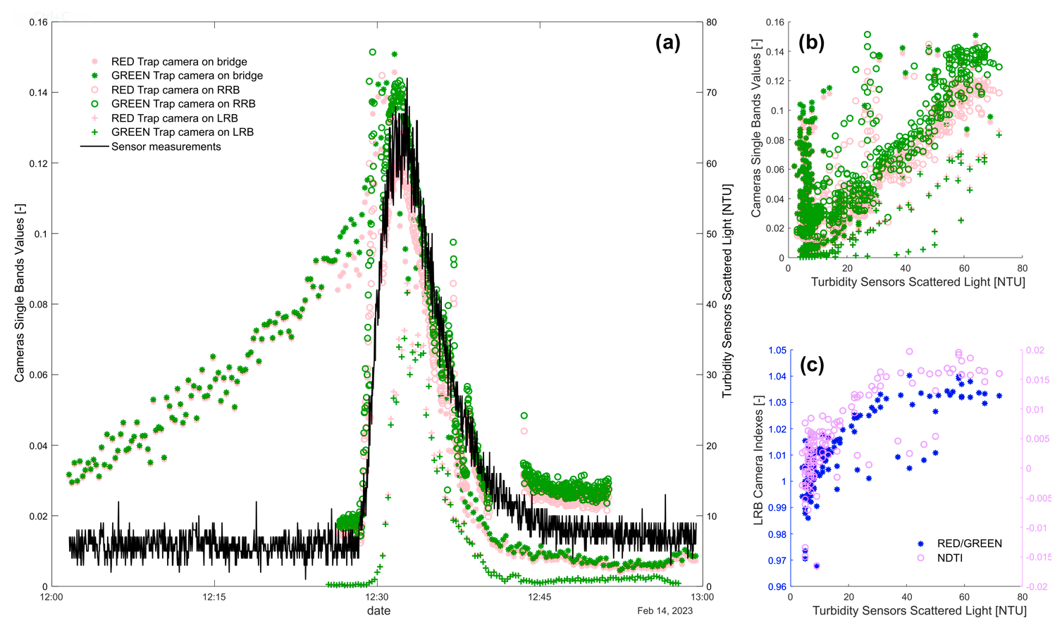
Figure 12 (a) Comparison between turbidimeter measurements and red- and green-band values from all of the trap cameras installed on site. (b) Scatterplot of all of the cameras' green-band signals and red-band signals. (c) Scatterplot of the NDTI and red and green indexes from the trap camera installed on the left riverbank (LRB). The colour schemes used in this figure are accessible to persons with colour vision deficiencies.

Trap camera outcomes are reported in Fig. 12, where it is possible to observe different patterns depending on the installation position. Red- and green-band signals, from the TCs installed on the LRB and RRB, follow the measurement curve for the entire monitoring period, while the TC installed on the bridge seems to be influenced by the variation in the light conditions during the first part of the experiment before exceeding turbidity values higher than 50 NTU. Moreover, all of the TC results show the same intensity values, in correspondence with the turbidity peak, except those from the LRB, matching the measures but with lower PI signals. The most reliable TC band ratios and indexes were those from the RRB position (Table 2).

The UAV camera returned partial data (Fig. 13) due to the loss of signal that caused a break in the recordings for 5 min immediately after reaching the measured turbidity peak. Therefore, there is good correspondence between the UAV band signal and the turbidimeter data. In the second part of the recording, we can observe that the band signals are lower than those during the peak, but they do not exactly fit the measurements' decreasing curve. This is because the white balance setting of the camera was on, and this resulted in a discrepancy in terms of the intensity of the starting signals but not in terms of variations.

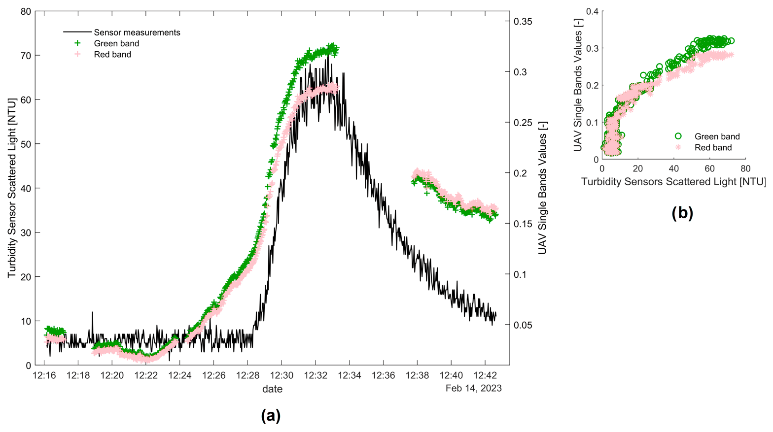
Figure 13 (a) Comparison between turbidimeter measurements and data from the UAV camera. (b) Scatter plot of the variables. The colour schemes used in this figure are accessible to persons with colour vision deficiencies.

3.1 Performance metrics

Table 2 summarises the performance in terms of linear and quadratic R-squared correlation coefficients, considering the different camera types, bands, view angles and installation setups selected for the field tests.

Table 2 Linear and quadratic correlation coefficients R² of the camera bands compared to turbidity measurements, considering different camera types and installation points selected for the experiment.

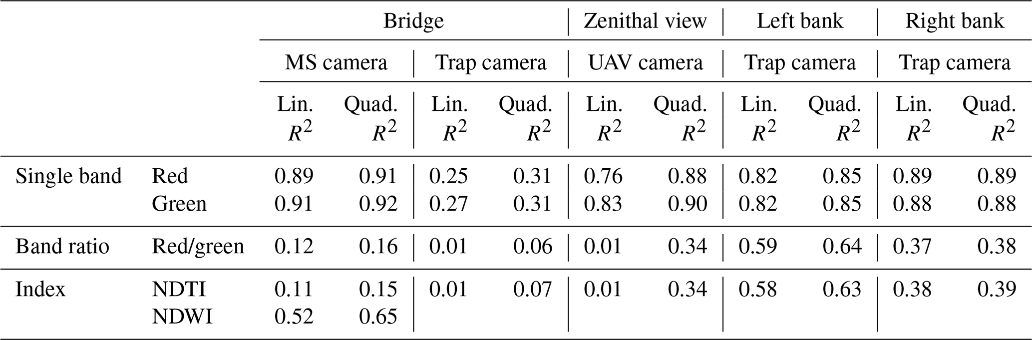
Single red and green bands can describe turbidity variations better than band ratios and indexes for all of the cameras used in this short-term experiment. Moreover, the MSC installation allowed us to understand the potential uses of bands beyond the visible spectrum. The NIR band seems to show good performance for a high concentration of suspended particles that reflect a consistent part of its radiation. In fact, considering combined MSC bands, the best performance comes from the NDWI index that involves the NIR and green bands.

4 Discussion

To enable a proper comparison of all of the variables, we decided to normalise them, as shown in Fig. 14, since the data came from several sources, such as turbidity sensors and camera bands. The min–max normalisation was chosen as the most suitable technique for our analysis because it scales the variables to a common range from 0 to 1, enabling direct comparison of their trends despite differences in units and ranges. This helps to highlight correlations between the turbidity sensor readings and camera outputs during the turbidity event, preserving the shape of the original distributions and maintaining relative relationships between data points.

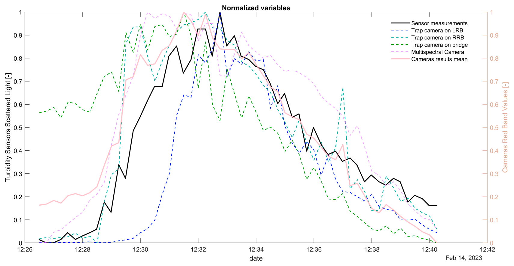
Figure 14 Comparison of normalised turbidimeter measurements and camera red-band values during the short-term experiment of February 2023. The colour schemes used in this figure are accessible to persons with colour vision deficiencies.

Within Fig. 14, the mean of all of the normalised camera band values is also reported in red. The normalisation made it easier to assess camera performances in relation to the measurements of turbidity. Additionally, it enables a consistent comparison among different camera types, avoiding the issue of the Bayer pattern, as used in digital cameras, which provides us with RGB values already interpolated, unlike the multispectral camera that measures pure bands.

Figure 15 describes the performance during the synthetic turbidity event of February 2023, focusing on the precision and accuracy of the normalised variables. The precision refers to the absolute difference between the turbidimeter measures and the camera data, while the accuracy is this difference divided by the measures, representing the percentage of the error. In particular, Fig. 15a shows the precision of the mean of the normalised camera bands. The red dots in this picture show the lower discrepancy between the measures and the image data, pointing out higher reliability of the camera data in reflecting the turbidity levels during the peak time, from 12:29 to 12:39, for the actual increase in turbidity (NTU>20). Figure 15b describes the normalised red-band values for the five different cameras over the entire turbidity event. The results show that most cameras exhibit relatively similar means and ranges of values, except for the LRB TC, presenting lower values, though these are still aligned with the measures. Figure 15c–e highlight again the lower range of variability and the best matching of the camera data with the turbidity sensor readings during the peak time rather than over the entire event. Figure 15f illustrates the behaviour of normalised red-band values of the different camera types during the turbidity peak time. It shows notable variability between the cameras. On the one hand, MSC results display the largest spread, indicating lower accuracy than TCs. On the other hand, the MSC boxplot, together with the LRB TC, is the only one without outliers and points standing on the whiskers, explaining this strong correlation with measurements reported in Table 2.

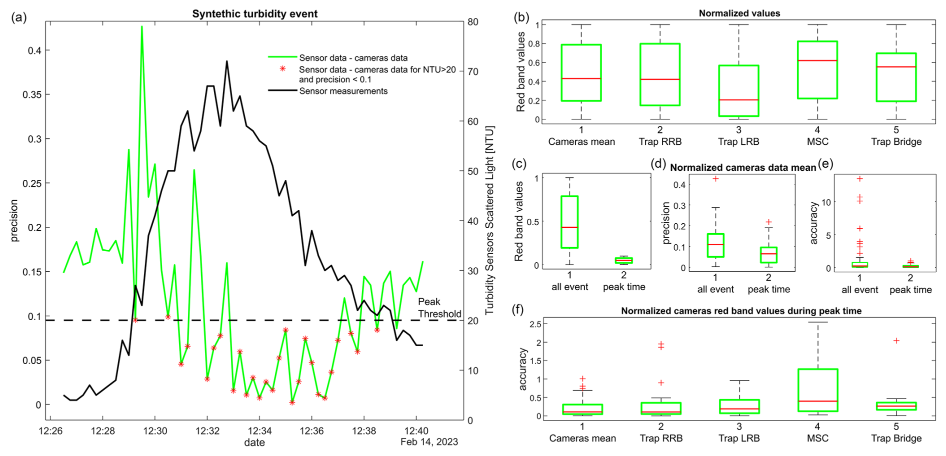
Figure 15 Plots of result precision (a, d) and accuracy (e, f) for each camera (b) considering the entire turbidity event and only the peak time (c–f) during the short-term experiment of February 2023. The colour schemes used in this figure are accessible to persons with colour vision deficiencies.

Overall, the results from both the short- and long-term data suggest to us that the camera lens sensibility is not the only factor to consider. Camera orientation, installation setups, available bands and also the intensity of the measured event can influence the monitoring performance.

Regarding the experimental setup, the presence of the submerged turbidimeters in both river sides (Fig. 4) ensured the quantification of the horizontal variability of the turbidity level along the river cross-section. The vertical variability of turbidity on the water column is not so significant for a river as small as the Selke, with a registered maximum water level of 1 m. However, the proposed image-based procedure will also apply for bigger rivers since cameras capture the light from the entire water column until a middle to high turbidity level is reached. Once this threshold is reached (see Fig. 3b), only the water surface can be investigated by the camera.

Interesting results were observed for all three RGB bands since we used a white clay to increase the turbidity level. Further experiments with multiple tracers as inputs, changing the colours and particle concentrations, will help to gauge the effectiveness of the procedure. What we expect from a generalised application of the procedure, in light of this and past field test experiences (Miglino et al., 2022), is the greater reliability of the red band for variable suspended-particle characteristics and better performances in terms of band ratios and indexes for long-term monitoring under different hydrological conditions.

4.1 Range of applications

The comparison of all experimental data in Fig. 16a shows that the initial band signal responses were different for each camera, depending on lens sensitivity, position, field of view, angles from water surface and orientation with respect to the sun's apparent motion axis. One way to homogenise these results is to consider the increment of band signals, starting from a band signal for clear-water conditions, referred to as the image frame with a minimum measured NTU value. Figure 16b shows the increments between the red-band signals (red) for each frame and for the clear-water conditions (red₀). Since the UAV data were split into two distinct videos, some of the primary turbidity event occurred during the pause between the two recordings; hence, it was excluded. In addition, the UAV camera was the only one with a pre-set automatic light balance, making it impossible to integrate these data with the others.

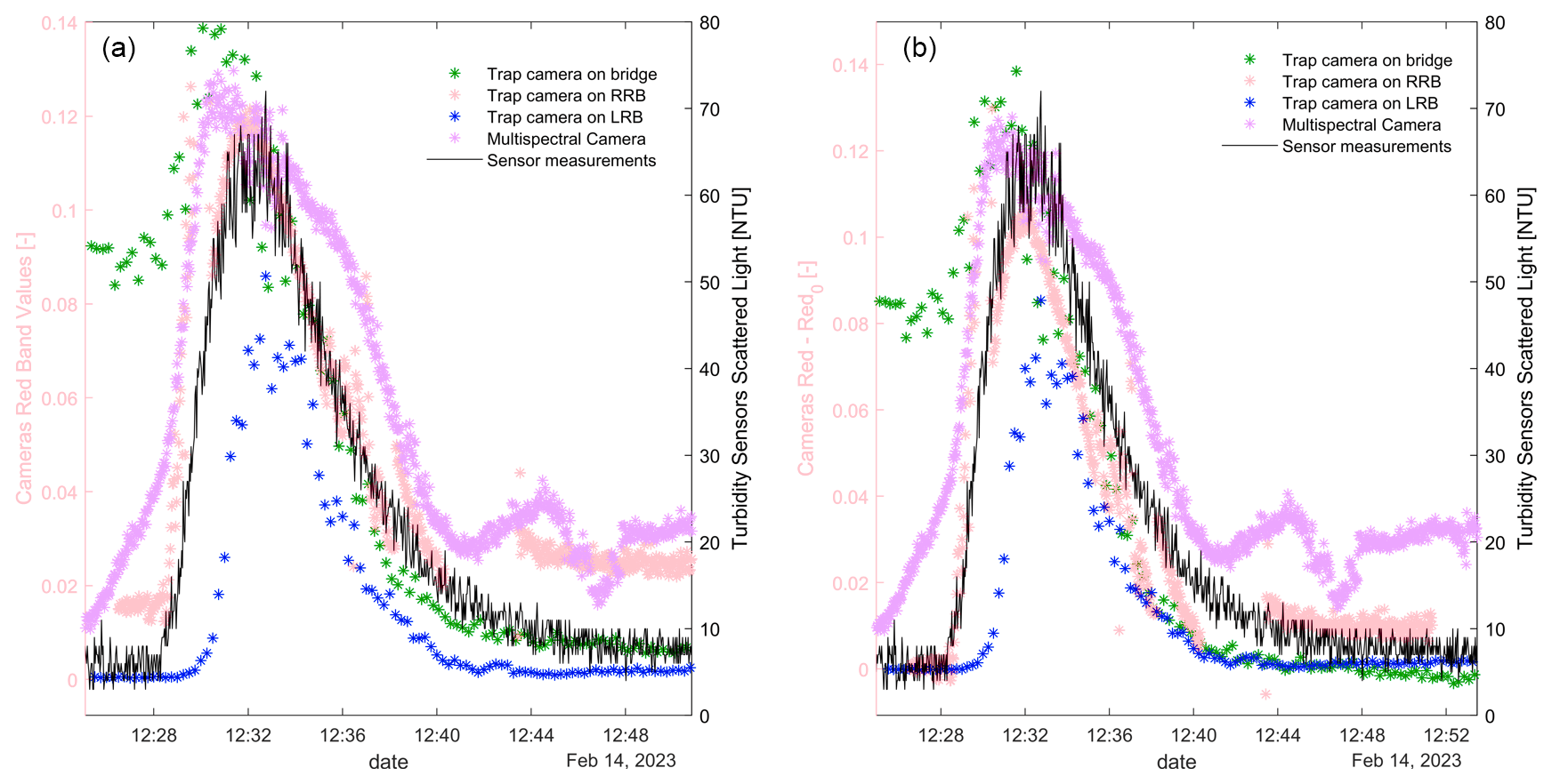
Figure 16 Comparison of turbidimeter measurements and all the cameras' data in terms of red-band values (a) and increments (b) starting from a clean-water condition (red₀). The colour schemes used in this figure are accessible to persons with colour vision deficiencies.

It is worthwhile to observe how there is a better overlap for the red–red₀ increment curves than for the single red-band signal curves. In fact, the identification of the PI for the clear water could remove the mismatches between the initial PIs detected by the camera due to both changes in light and camera lens sensitivity. Future experiments will face this issue, especially for shallow-water conditions, where the visibility of the riverbed background could become a reference value of water clarity, regardless of site- and time-specific variabilities.

4.2 Implications in river monitoring practices

Prior to this work, image analysis for water turbidity was predominantly conducted using satellite data for large rivers or through the use of camera data and specific optical sensors in the laboratory. The added value of our study lies in the development of a monitoring procedure that can be directly implemented on site. This allowed us to test the method under real conditions and to optimise the camera installation for future applications in various environments.

The proposed image-processing procedure offers significant advances in river monitoring practices by providing a near-real-time, continuous and automated system for water turbidity assessment. This approach can complement current monitoring practices, addressing their limitations in terms of data availability and resolution, especially for small or inaccessible rivers where existing methods are impracticable. Furthermore, the use of remote sensing technology minimises environmental disturbance, aligning with sustainable monitoring practices. The dissemination of this procedure could significantly increase the amount of available information on water status at the basin scale, thereby enhancing our understanding of the ecohydrological dynamics involved in river processes.

4.3 Spatial variability and active pixel count within the region of interest

In our investigations, only the mean of the active pixels within the ROI is considered as a proxy for turbidity. For active pixels, we refer to the processed pixels with information on the actual water reflectance. The image-processing procedure allowed us to minimise the misinformation from the images, reducing the effect of changing light conditions with radiometric calibration and removing saturated pixels or strongly shaded areas with binarisation. Nevertheless, the spatial variability of the pixel intensities and the availability of active pixels within the ROI of a single image could be critical factors that need to be analysed.

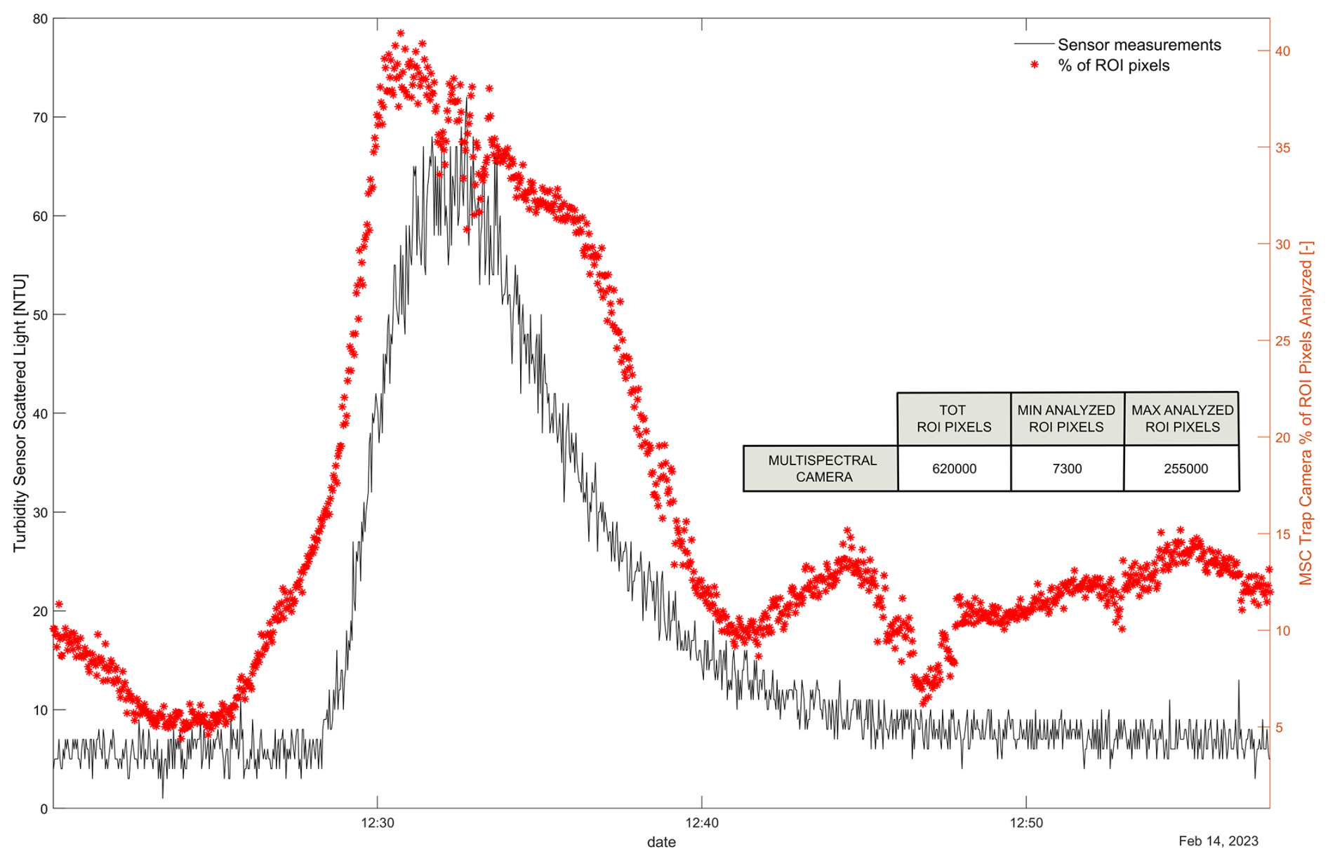
Figure 17 Comparison of turbidimeter measurements (line in black) and number of analysed ROI pixels in MSC data (“*” symbols in red) during the short-term experiment of February 2023

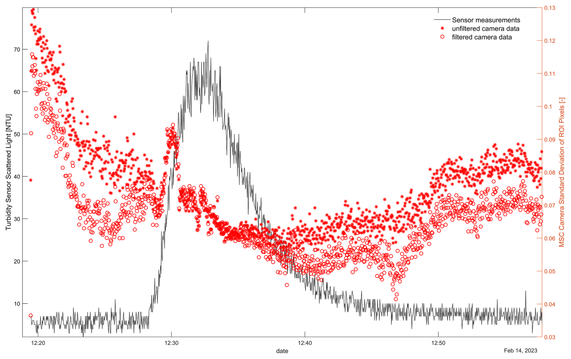
Figure 18 Comparison of turbidimeter measurements (line in black) and the standard deviation of ROI pixel intensity in multispectral-camera red-band filtered (“o” symbols in red) and unfiltered (“*” symbols in red) data during the short-term experiment of February 2023.

Figures 17–20 describe the variability of the standard deviation and the active pixel count for both the MSC and TC during the field experiment of February 2023.

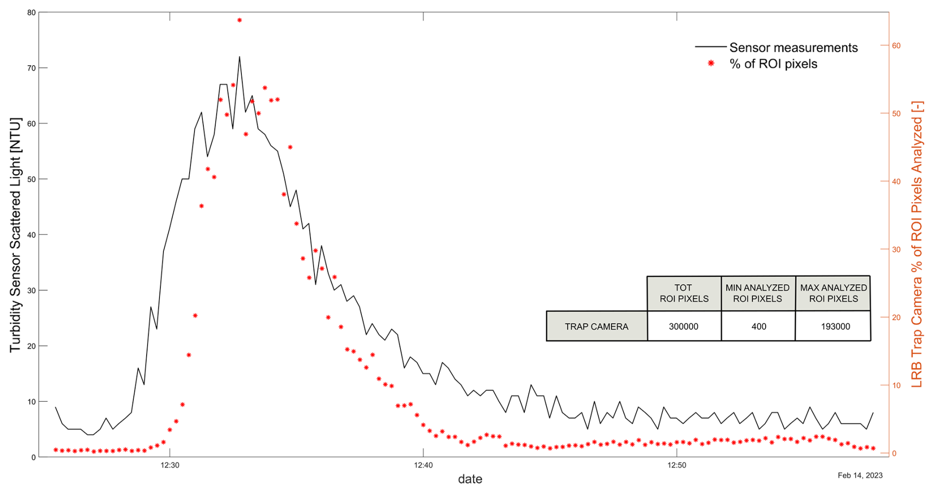
Figure 19 Comparison of turbidimeter measurements (line in black) and number of analysed ROI pixels in LRB trap camera data (“*” symbols in red) during the short-term experiment of February 2023.

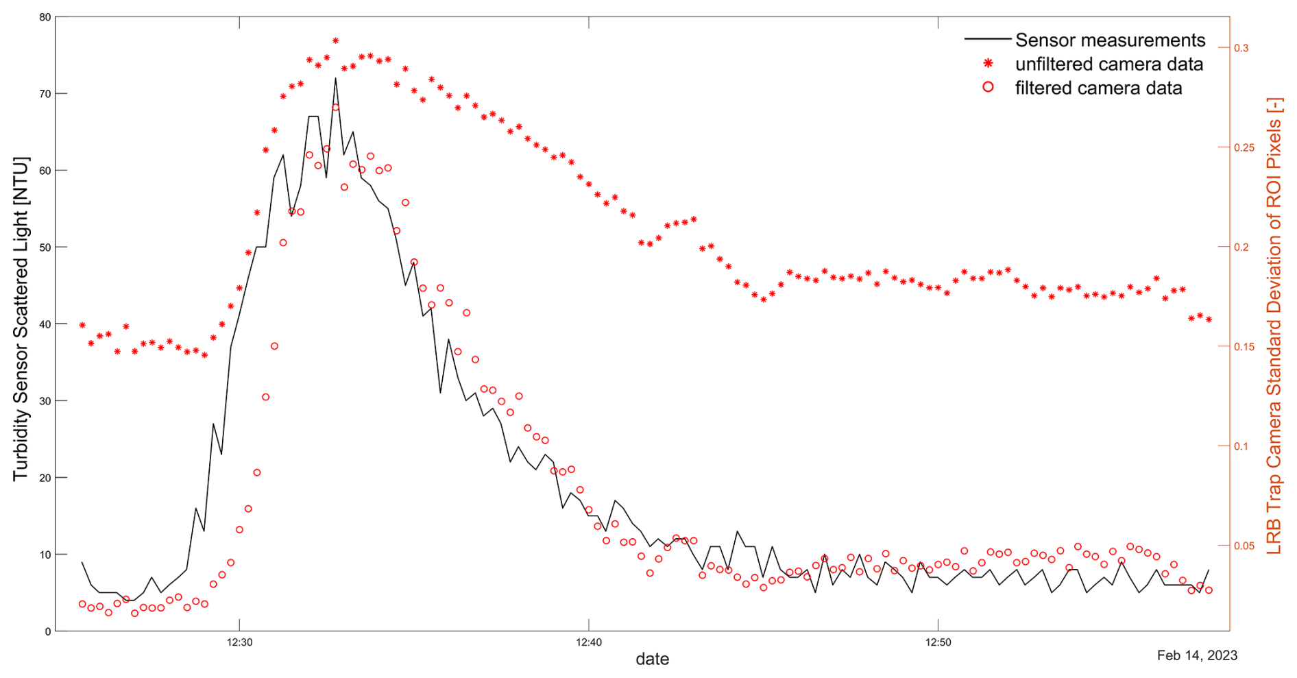
Figure 20 Comparison of turbidimeter measurements (line in black) and the standard deviation of ROI pixel intensity in LRB trap camera red-band filtered (“o”symbols in red) and unfiltered (“*”symbols in red) data during the short-term experiment of February 2023.

It is worthwhile to observe that the active pixel count is directly proportional to the turbidity level for both the MSC (Fig. 17) and trap camera (Fig. 19). These results show that the resolution of the camera and its distance from the water must be considered to ensure a minimum number of active pixels for less sensitive cameras, such as the trap camera, especially when the water is clear.

In Figs. 18 and 20, it is evident that the image-filtering procedure of the camera data significantly reduces the standard deviations of the ROI pixel intensity, particularly for low to moderate turbidity conditions, where its spatial variability is particularly high for the unfiltered data. Finally, these figures confirm the effectiveness of the procedure in enhancing the overall river turbidity level using cameras, even if the shown PI standard deviation values are still non-negligible.

5 Conclusions

The experimental activities revealed that single-band values were the most reliable proxy for turbidity monitoring in short-term observations, even more so than band ratios and indexes. The opposite could be true for long-term observations since single-band signals tend to be more influenced by the variability of light and flow conditions. The advantages of using this procedure are multiple. Field tests proved that cameras, even the cheap models, can produce reliable turbidity estimates continuously in time. Moreover, they can be easily installed in greater numbers than turbidimeters without the burden of cost along the river network, providing a comprehensive knowledge of the river basin status.

On-site tests are still on-going in two different case studies. In particular, in the Bode River, a trap camera is providing continuous long-term monitoring of actual turbidity events. This will allow us to acquire a significant set of data, covering many environmental and hydrological conditions, to fully understand how to optimise the characteristics of the camera and the installation setups for real monitoring applications. Moreover, another camera has been installed in the Sarno River section, within the scope of our RiverWatch research project activities. This is a relevant case study to outline innovative and effective guidelines for water quality monitoring and water pollution prevention, with the study site being one of the most polluted rivers in Europe, directly involving us. The practical application of this image-based procedure could create an innovative early-warning network that is not limited to turbidity but also proves to be of great potential for other water-quality- (e.g. chlorophyll a) and water-related (e.g. macroplastics) monitoring applications (Manfreda et al., 2024), advancing and supporting the existing river monitoring techniques. The next natural step is the involvement of these water quality estimation algorithms in a citizen science approach. Within this context, our research group is developing a smartphone app for river monitoring (https://sites.google.com/view/riverwatch/home-page?authuser=0, last access: 1 September 2025), focusing, in particular, on macroplastics and turbidity, which constitute the most easy to capture water quality information collectable by the people. The real implementation of a continuous image-based river monitoring network like this can offer new options to water resource management strategies and the preservation of aquatic ecosystems.

Appendix A: List of abbreviations

Abbreviation	Description
LRB	Left riverbank
MSC	Multispectral camera
NTU	Nephelometric turbidity unit
RCP	Radiometric calibration panel
RGB	Red, green and blue: colour representation model used on the digital screen
ROI	Region of interest
RRB	Right riverbank
TC	Trap camera
UAV	Uncrewed aerial vehicle
WT	Water turbidity
DN	Digital number (–)
PI	Pixel intensity (–)
IR	Solar irradiance (W m−2)
NDTI	Normalised difference turbidity index (–)
NDWI	Normalised difference water index (–)
NIR	Near-infrared radiation band (0.78–3 µm)
Rb	Reflectance of the riverbed background (–)
Red0–red	Band value for clear-water condition (–)
RVrc	RGB band reference value of the radiometric calibration panel (–)
Rs	Reflectance of the suspended particles (–)
Rw	Reflectance of the water (–)
SSC	Suspended-sediment concentration (g L−1)