Enhanced hydrological modeling with the WRF-Hydro lake–reservoir module at a convection-permitting scale: a case study of the Tana River basin in East Africa

East Africa frequently experiences extreme hydrological events, such as droughts and floods, underscoring the urgent need for improved hydrological simulations to enhance prediction accuracy and mitigate losses. A major challenge lies in the limited quality of precipitation data and constraints on model capabilities. To address these challenges, the upper and middle Tana River basin, characterized by its sensitivity to drought, vulnerability to flooding, and data availability, was selected as a case study. We performed convection-permitting (CP) regional climate simulations using the Weather Research and Forecasting (WRF) model and conducted hydrological simulations with a lake–reservoir-integrated WRF Hydrological modeling system (WRF-Hydro) driven by the CPWRF outputs. Our results show that the CPWRF-simulated precipitation outperforms ERA5 when benchmarked against Integrated Multi-satellite Retrievals for GPM (Global Precipitation Measurement) (IMERG), with evident bias reduction in seasonal precipitation mainly over the Mount Kenya region and with a probability of light rainfall (1–15 mm d⁻¹) during the dry season. Improved precipitation enhances the hydrological simulation, significantly reducing false peak occurrences and increasing the Nash–Sutcliffe efficiency (NSE) by 0.53 in the calibrated lake-integrated WRF-Hydro model (LakeCal) driven by CPWRF output compared to ERA5-driven simulations. Additionally, the lake–reservoir module increases the sensitivity of river discharge to spin-up time and affects discharge through lake–reservoir-related parameters, although adjustments to the parameters (i.e., the runoff infiltration rate, Manning's roughness coefficient, and the groundwater component) have minimal effects on discharge, particularly during the dry season. The inclusion of the lake–reservoir module effectively reduces the model-data bias in WRF-Hydro simulations, particularly for the dry-season flow and peak flow, resulting in an NSE increase of 1.67 between LakeCal and LakeNan (model without the lake–reservoir module). Notably, 24 % of the NSE improvement is attributed to CPWRF and 76 % is attributed to the lake–reservoir module. These findings highlight the enhanced capability of hydrological modeling when combining CPWRF simulations with the lake–reservoir module, providing a valuable tool for improving flood and drought predictability in data-scarce regions like East Africa.

1 Introduction

The credibility of hydrological simulations in data-scarce regions is challenged by the limited quality of precipitation data (e.g., incomplete, unreliable, and poor in situ coverage) and the constrained capacity of the hydrological model given the underlay's complexities. To make well-informed decisions concerning flood/drought adaptation and loss mitigation, elected officials, planners, and the public require relatively reliable information on flood and drought forecasts, which rely on skilled hydrological simulations. This issue could be particularly acute in drought-/flood-prone and vulnerable areas such as East Africa. The economy and population in East Africa mainly depend on rain-fed agriculture and pastoralism, which suffer from frequent droughts and floods (Taye and Dyer, 2024). For example, the drought of 2022 triggered an exceptional food security crisis in Ethiopia, Somalia, and Kenya, pushing more than 20 million people into extreme hunger (NASA, 2022). Similarly, the flood in 2023 here killed more than 100 people and displaced over 700 000 (NASA, 2024). The highlighted risk in East Africa requires effective hydrological simulation for better hydrological extreme forecasts, thus supporting effective water resource planning and management and aiding informed decision-making and loss mitigation for officials, planners, and the public.

Obtaining even the present-day precipitation, especially in mountainous regions, is challenging due to poor in situ coverage and incomplete or unreliable records. Such data scarcity even complicates the evaluation of model output (Li et al., 2017). This issue is only further exacerbated as grid spacing is decreased to kilometer scales. Gridded precipitation production tried to be an alternative to address some of the data scarcity issues. These gridded products include merged data such as Climate Hazards Group InfraRed Precipitation with Station data (CHIRPS) (Funk et al., 2015), reanalysis data like ERA-Interim (Dee et al., 2011), and satellite-based data involving the Tropical Rainfall Measuring Mission (TRMM) (Adjei et al., 2015) and Integrated Multi-satellite Retrievals for GPM (Global Precipitation Measurement) (IMERG) (Dezfuli et al., 2017). However, these products present uncertainties, such as the false detection of precipitation events and biases of precipitation amounts (Bitew and Gebremichael, 2011; Ma et al., 2018; Dezfuli et al., 2017), which limit their suitability for hydrometeorological application. These uncertainties are particularly pronounced in mountainous regions (Li et al., 2018; Maranan et al., 2020; Zandler et al., 2019). Also, precipitation from coarse-resolution global climate models has its limitations (Monsieurs et al., 2018; Kad et al., 2023), primarily due to the model configuration, such as resolution and parameterization, which is crucial for a more realistic representation of processes (Kad et al., 2023; Tao et al., 2020).

Dynamical downscaling models offer a promising tool for generating precipitation patterns with realistic regional detail. They can capture refined-scale features such as topography and local processes that influence orographic effects (Kad and Ha, 2023; Tao et al., 2020). The study by Kerandi et al. (2017) highlights the importance of using higher-resolution models for more accurate climate features. The Weather Research and Forecasting (WRF) model with a refined resolution of 25 km captures the temporal variability on interannual to annual scales, and the spatial distribution of precipitation in the Tana River basin is more effectively represented than the coarser 50 km resolution. Indeed, at relatively coarse resolution (such as >20 km resolution), regional climate models (RCMs) generally struggle to adequately represent precipitation and exhibit uncertainties when compared to reanalysis data, rain gauges, and satellite observations (Biskop et al., 2012; Ji and Kang, 2013). A refined horizontal resolution can significantly improve precipitation simulation over equatorial East Africa (Pohl et al., 2011).

Convection-permitting regional climate models (CPRCMs; typically with a resolution of <5 km) provide an explicit representation of convection, allowing for capturing local-scale precipitation extremes. This is a clear advantage over coarser resolutions (Kendon et al., 2021; Schwartz, 2014; Weusthoff et al., 2010). The added value of CPRCMs compared to the parameterized regional climate models includes improved representations of the intensity distribution (Tucker et al., 2022; Berthou et al., 2019), diurnal cycle (Stratton et al., 2018), and storm size and duration (Crook et al., 2019). It is noteworthy that CPRCMs better capture surface heterogeneities and produce more realistic climate simulations over mountainous regions (Kawase et al., 2013; Rasmussen et al., 2014). Furthermore, CPRCMs show increased performance over Africa (Tucker et al., 2022) in presenting rainy events, diurnal cycle, and peak time for the Lake Victoria basin of East Africa (van Lipzig et al., 2023), as well as sub-daily rainfall intensity distribution, especially that related to convective rainfall in the tropics (Folwell et al., 2022). Therefore, CPRCM holds promise for generating more realistic precipitation with regional details in East Africa.

Atmospheric–hydrological modeling is a common approach for simulating and predicting climate extremes such as floods and droughts. While regional climate model (RCM) outputs are often directly used in hydrological studies, they may introduce inconsistency due to mismatches in spatial and temporal scales or biases in the simulated atmospheric processes (Chen et al., 2011; Teutschbein and Seibert, 2012). A better approach would be to couple atmospheric and hydrological modeling systems to ensure physical consistency. A coupling of the Weather Research and Forecasting (WRF) model and the WRF Hydrological modeling system (WRF-Hydro; Gochis et al., 2018) shows advantages in hydrology simulations and forecasting hydrological extremes globally (e.g., Kerandi et al., 2018; Li et al., 2017), including urban flood prediction over the Dallas–Fort Worth area of North America (Nearing et al., 2024) and drought estimation in South Korea (Alavoine and Grenier, 2023). In Africa, WRF-Hydro has also proven useful for discharge simulations in the Ouémé River of West Africa (Quenum et al., 2022) and the Tana River basin (Kerandi et al., 2018). Kerandi's study demonstrated minimal differences in precipitation between the stand-alone and fully coupled models, which suggests that precipitation recycling and land–atmosphere feedback have a limited impact on soil moisture and discharge in the Tana River basin. Similar findings have been observed in other regions, such as the Crati River basin in southern Italy (Senatore et al., 2015) and the United Arab Emirates (Wehbe et al., 2019).

Although WRF-Hydro shows potential, its application in East Africa requires refinement through the implementation of more comprehensive hydrological processes. Numerous reservoirs have been constructed in East Africa (Palmieri et al., 2003), altering the magnitude and timing of natural streamflow. These reservoirs typically attenuate and delay flows during the rainy season, while they release water during the dry season (Zajac et al., 2017; Hanasaki et al., 2006). Incorporating lake–reservoir processes in hydrological simulation is essential for creating reliable models in regions with lakes (Hanasaki et al., 2006; Lehner et al., 2011). However, only a few hydrological simulations over East Africa are related to lakes (Oludhe et al., 2013; Naabil et al., 2017; Siderius et al., 2018), and even fewer studies have examined the impact of reservoirs in this region, particularly in cases where meteorological and hydrological models are coupled. Naabil et al. (2017) used WRF-Hydro with the dam water balance model for dam level simulation and water resource assessment in the Tono dam basin but did not include the reservoir module in the WRF-Hydro system, limiting the accurate capture of the dam's impact on discharge and other hydrological variables. Therefore, hydrological modeling coupled with its lake–reservoir module is required for reliable flood and drought simulations over East Africa. While the WRF-Hydro system, integrated with the lake–reservoir module, shows promise for simulating the water balance affected by reservoirs (Maingi and Marsh, 2002), its use in East Africa, especially in large river basins like the Tana River, remains limited.

The Tana River basin in East Africa is ideal for enhanced hydrological modeling due to its proneness and vulnerability to droughts and floods, as well as the availability of observational data. These discharge records provide a benchmark for simulations despite some uncertainties. The basin supports vital ecosystem services for Kenya, including drinking water supply, hydroelectric power generation, agriculture, and biodiversity, and is home to over 8 million people (Lange et al., 2015). However, the region is observed to be at risk of drought and flooding, which are likely exacerbated by climate change (Kenya Climate Change Case Study, 2024). Droughts occur approximately every 5 years, causing shortages of water for drinking, irrigation, and fishing (Bonekamp et al., 2018). The 2018 flood overflowed the riverbanks, damaging crops, homes, and infrastructure; displacing thousands of people; and contributing to outbreaks of waterborne diseases such as cholera (Kiptum et al., 2024). Robust hydrological modeling in the Tana River basin is essential for accurate predictions of extreme events and practical risk assessment. Using the Tana River basin as a case study, our research aims to address some of the issues related to flood and drought risk mitigation, through a more comprehensive hydrological simulation with a convection-permitting WRF model and lake–reservoir-integrated WRF-Hydro system. We target the following sub-objectives: (1) to improve climate output (particularly focusing on precipitation) through convection-permitting (CP) WRF simulation (CPWRF) and using the enhanced precipitation representation to advance the hydrological simulation, (2) to explore the potential of the lake–reservoir module to improve hydrological simulation skill, and (3) to build an enhanced WRF-Hydro system and investigate the contribution of (1) the CPWRF simulation and (2) the lake–reservoir module to hydrological simulation improvement. The research aims to improve hydrological models, which helps to better water resource management and risk mitigation, and supports sustainable practices in regions vulnerable to water-related damage.

2 Study area and data

The Tana River basin, located in the tropics, exhibits dual peaks in precipitation due to the biannual migration of the Intertropical Convergence Zone (ITCZ). The spatial distribution of precipitation is profoundly modulated by the basin's varied topography and atmospheric deep convection (Kad et al., 2023; Johnston et al., 2018), which results in a gradient condition ranging from arid in the lowlands to semi-humid in the highlands and coastal areas (Knoop et al., 2012). The precipitation pattern is also influenced by the El Niño–Southern Oscillation (Otieno and Anyah, 2013; Anyah and Semazzi, 2006), Indian Ocean Dipole (IOD) (Williams and Funk, 2011), and rising atmospheric CO₂ (Kad et al., 2023).

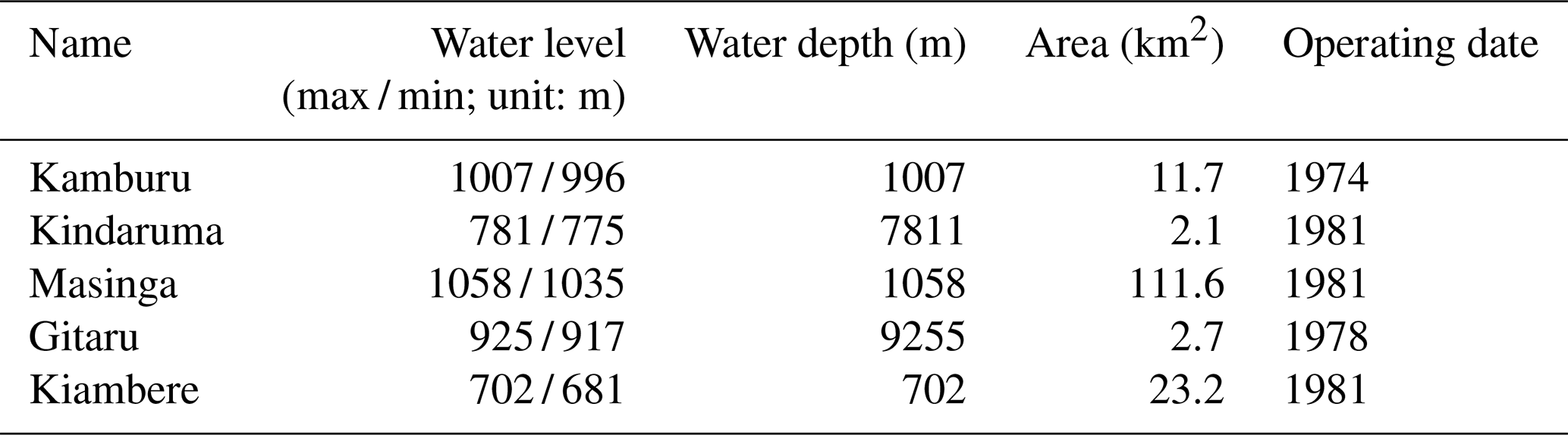
Our study focuses on the upper and middle Tana River basin (TRB), covering an area of 32 865 km² upstream of the city of Garissa (1.25° S–0.50° N and 36.50–39.75° E). This region includes famous mountain ranges, such as the Mount Kenya massif and the Aberdare Range, alongside plain surfaces (Fig. 1b). The region is characterized by a complex interplay of mountainous terrain and a flat surface, with elevation ranging from 34 to in excess of 4800 m (Fig. 1a). To analyze and evaluate the spatial distribution of precipitation concerning the topography, we classified the terrain into mountainous regions above 1600 m and plains below 1600 m. There are five reservoirs in the basin along the Tana River, including Masinga, Kamburu, Gitaru, Kindaruma, and Kiambere from the upstream to downstream (Table 1 and Fig. 1c). These five lakes are between Garissa station upstream and Rukanga downstream. It is important to note that the lakes do not affect the streamflow at Rukanga, but they do impact the discharge at Garissa.

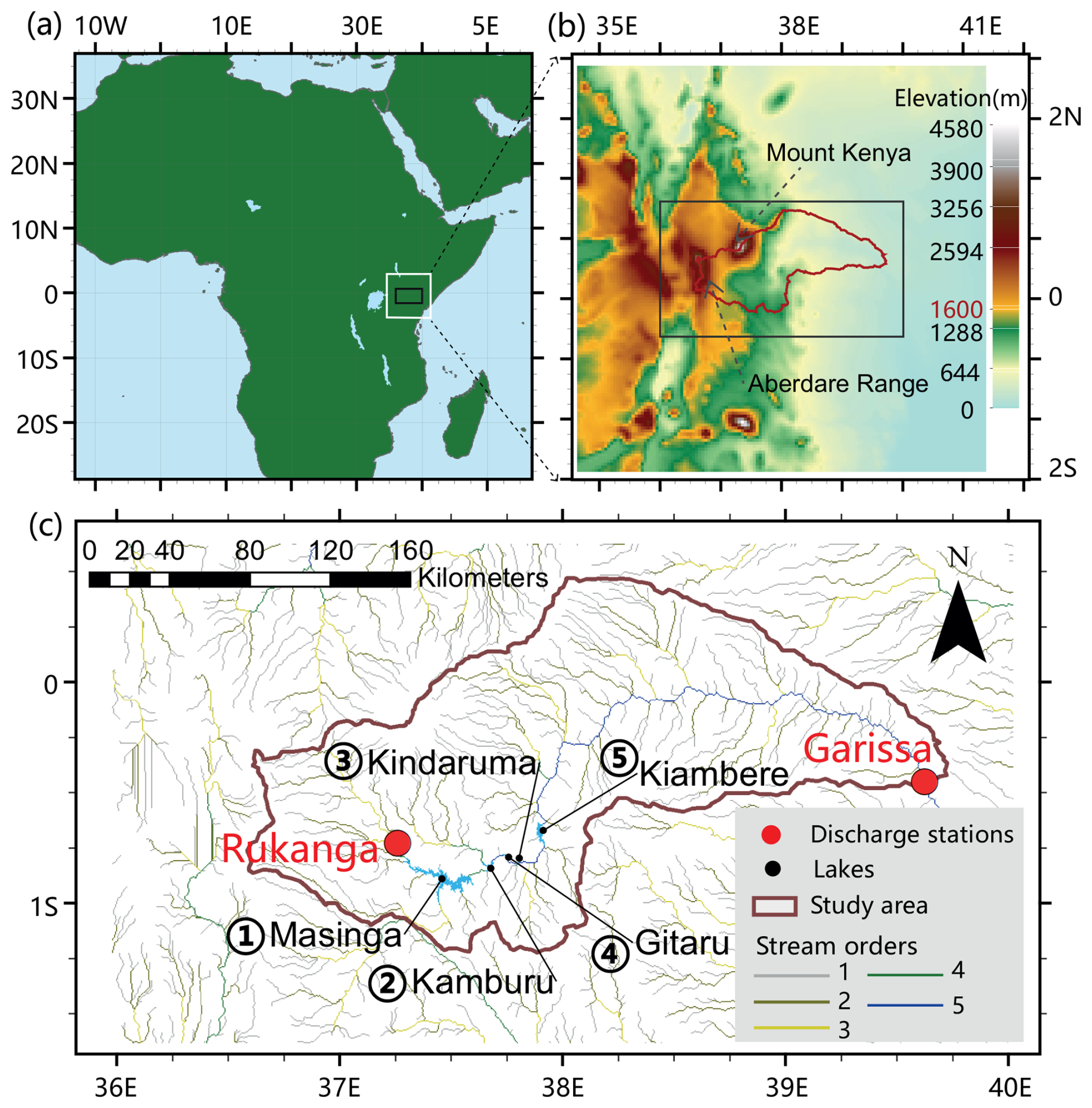
Figure 1 Study basin location in East Africa. (a) The WRF domain with a resolution of 5 km (shown with the white frame) and the location of the inner region (a black frame) used as the domain of the WRF-Hydro simulation. (b) A zoomed-in view of the inner area showing topography, two major mountains, and the basin boundary. (c) Drainage map of the upper and middle Tana River basin, including the discharge stations, lake–reservoir water level stations, and stream orders for hydrological modeling in the WRF-Hydro model system.

Table 1 Lakes in the upper and middle Tana River basin (TRB).

Here, we used the global satellite product of GPM_3IMERGDF (GPM IMERG precipitation version 6 at daily temporal resolution and 0.1°×0.1° spatial resolution) (Huffman et al., 2020) for CPWRF precipitation evaluation, downloaded from the NASA website (https://gpm.nasa.gov/data-access/downloads/gpm, last access: 28 April 2023). These climate data cover the period 2010–2014. Discharge observations during 2011–2014 at two stations in the TRB (Garissa and Rukanga), obtained from the Water Resources Authority of Kenya (WRA), are used for WRF-Hydro model discharge sensitivity analysis and calibration (Fig. 1).

3 Methodology

3.1 WRF domain design for convection-permitting modeling

To obtain convection-permitting regional climate model simulations, we used the Advanced Research WRF (WRF-ARW) model version 4.4 (Skamarock et al., 2019) with the designed domain of 5 km spatial resolution (Fig. 1). The lateral boundaries were forced with the 6-hourly ERA5 reanalysis with a spatial resolution of 0.25° (Hersbach et al., 2020). The model was set with 50 vertical levels up to 10 hPa. The convection parameterization was turned off for the CPWRF simulation, the Mellor–Yamada–Nakanishi–Niino Level 2.5 (MYNN2.5) scheme (Nakanishi and Niino, 2006) was used for the planetary boundary layer, the Rapid Radiative Transfer Model (RRTM) scheme was used for longwave radiation (Mlawer et al., 1997), and the Dudhia shortwave scheme was used for shortwave radiation (Dudhia, 1989). The Noah-Multiparameterization land surface model (Noah-MP LSM; Yang et al., 2011) was used for the land surface scheme.

The model runs from 1 January 2010 to 31 December 2014. Typically, WRF simulations require a spin-up of about 1 month, which should ideally be excluded from precipitation evaluation. However, given the limited length of simulated precipitation, the subsequent analysis is based on the full precipitation simulation from January 2010 to December 2014.

3.2 Sensitivity analysis and calibration strategy for WRF-Hydro modeling

3.2.1 WRF-Hydro modeling and preliminary calibration

For hydrological modeling, the WRF-Hydro system version 5.3 (Gochis et al., 2018) was employed in an offline mode, driven by the CPWRF atmospheric data within a domain at 5 km resolution with 90×50 pixels over the TRB (Fig. 1). The sub-grid routing processes were executed at a 500 m grid spacing, and surface physiographic files were generated by ArcGIS 10.6 (Sampson and Gochis, 2015). The physiographic files included high-resolution terrain grids (that specified the topography), channel grids, flow direction, stream order (for channel routing), a groundwater basin mask, and the position of stream gauging stations. The first five stream orders and gauging stations are shown in Fig. 1c. We activated the saturated subsurface overflow routing, surface overland flow routing, channel routing, and baseflow modules. The overland flow routing and channel routing were calculated by a 2-D diffusive wave formulation (Julien et al., 1995) and a 1-D variable time-stepping diffusive wave formulation, respectively.

The model involves the five lake–reservoir systems using a level-pool lake–reservoir module, which calculates both orifice and weir outflow. Fluxes into a lake–reservoir object occur when the channel network intersects a lake–reservoir object. The level-pool scheme tracks water elevation over time, and water exits the lake–reservoir system through either weir overflow (Outflow_w) or orifice-controlled flow (Outflow_o), as described by Eqs. (1) and (2).

$$\begin{array}{}\text{(1)}& {\text{Outflow}}_{\mathrm{w}}=\left\{\begin{array}{ll}{C}_{\mathrm{w}}L{h}^{\mathrm{3}/\mathrm{2}},& h>h_{\text{max}}\\ \mathrm{0},& h\le h_{\text{max}},\end{array}\right.\end{array}$$

where h is the water elevation (m), h_max is the maximum height before the weir begins to spill (m), C_w is the weir coefficient, and L is the length of the weir (m).

$$\begin{array}{}\text{(2)}& {\text{Outflow}}_{\mathrm{o}}=C_{\mathrm{o}}{S}_{\mathrm{o}}\sqrt{\mathrm{2}gh},\end{array}$$

where C_o is the orifice coefficient, S_o is the orifice area (m²), and g is the acceleration of gravity (m s⁻²).

For sensitivity analysis and model optimization, we initially calibrated the WRF-Hydro system without the lake–reservoir system (with the lake–reservoir module inactive). Two key hydrological parameters, REFKDT and MannN, were tuned using the auto-calibration Parameter Estimation Tool (PEST; http://www.pesthomepage.org, last access: 23 August 2025). The optimization is performed by maximizing the accuracy of the discharge simulation, indicated by the Nash–Sutcliffe efficiency (NSE) coefficient (Nash and Sutcliffe, 1970) of simulated discharge against the observation at Garissa. The calibrated WRF-Hydro model without the lake–reservoir system is referred to as LakeNan in the following analysis.

3.2.2 Experiments designed for sensitivity analysis in WRF-Hydro modeling with the lake–reservoir module

To optimize WRF-Hydro modeling over the TRB, we facilitated a comprehensive sensitivity analysis, involving spin-up time, hydrological parameters, groundwater components, and lake–reservoir-related parameters. Groundwater component tuning focuses on the parameter GWBASEWCTRT (an option for groundwater mode). Hydrological parameters include the Manning roughness parameter (MannN) and runoff infiltration coefficients (REFKDT). Lake–reservoir-related parameters cover the elevation of the maximum lake–reservoir height (LkMxE; unit: m), weir elevation (WeirE; unit: m), weir coefficient (WeirC; ranging from 0 to 1), weir length (WeirL; unit: m), orifice area (OrificeA; unit: m²), orifice coefficient (OrificeC; ranging from 0 to 1), orifice elevation (OrificeE; unit: m), and lake–reservoir module area (LkArea; unit: m²).

For sensitivity analysis of specific parameters, a set of experiments were conducted. In each experiment, only the parameter of interest was changed, while all others were kept at their defaults (Table 2). The defaults of lake–reservoir-related parameters were obtained from the WRF-Hydro GIS pre-processing toolkit (Gochis et al., 2018), while the others were derived from the preliminary calibrated WRF-Hydro system without the lake–reservoir module (LakeNan, Sect. 3.2.1).

Table 2 The default values for sensitivity experiments.

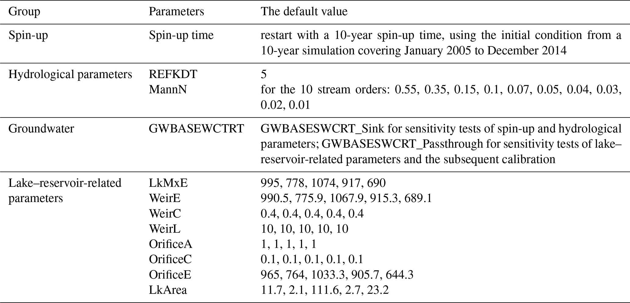
The default values for REFKDT and MannN are from the preliminary calibration of the LakeNan model (WRF-Hydro system without the lake–reservoir module). The MannN value is different for each stream order from 1 to 10. The values are listed in order for the five reservoirs of Kamburu, Kindaruma, Masinga, Gitaru, and Kiambere, respectively, obtained from the WRF-Hydro GIS pre-processing toolkit. The parameter GWBASEWCTRT is used to configure the groundwater component, involving two options in our experiments. One option creates a sink at the bottom of the soil column, where water draining from the soil exits the system. The other option bypasses the bucket model, directly transferring all drainage from the bottom of the soil column into the channel. These two options are referred to as GWBASEWCTRT_Sink and GWBASEWCTRT_Passthrough, respectively, throughout the paper.

Sensitivity to spin-up time

To obtain a stable hydrological simulation, spin-up time is required. Insufficient spin-up for initialization can introduce unnecessary uncertainties, potentially compromising the accuracy of subsequent sensitivity analyses and hydrological modeling assessments. Previous studies have demonstrated that spin-up time influences initial conditions such as the soil moisture content, surface water, the lake–reservoir module water level, and groundwater, which potentially influences the fidelity of model simulations (Ajami et al., 2014a, b; Bonekamp et al., 2018; Seck et al., 2015), subsequently affecting the result of subsequent sensitivity analyses and the performance of the hydrological simulation. For example, groundwater simulation may require more than 10 years of spin-up to reach stability (Ajami et al., 2014b). Since the shortest spin-up time likely depends on the quality of the model input (especially soil data) and local conditions, the impact of spin-up time needs to be assessed on a case-by-case basis. Therefore, we first investigated the sensitivity of spin-up time to identify the shortest duration required for achieving model stability and ensuring computational efficiency.

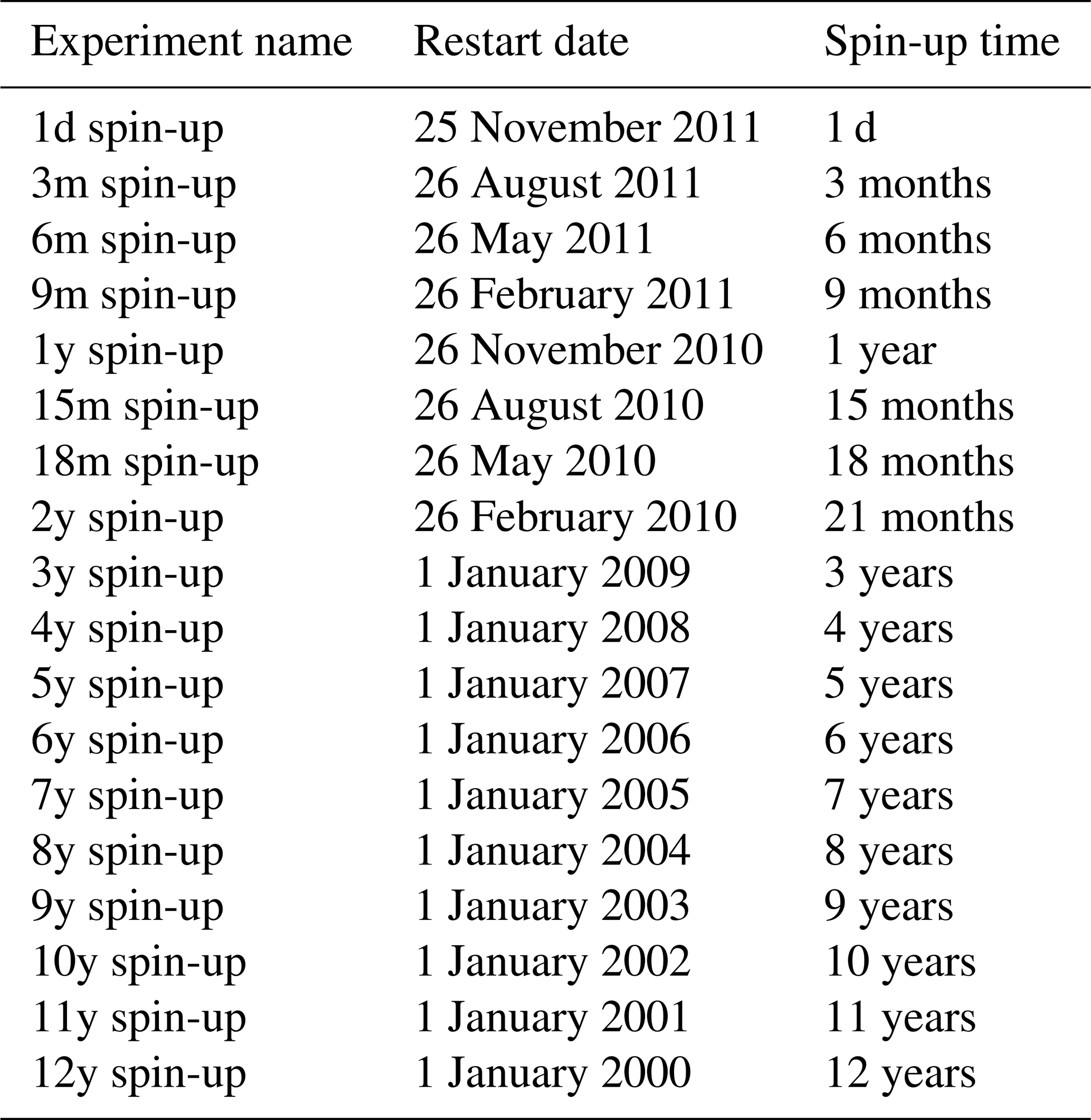
In our study, we conduct experiments of 17 different spin-up times (Table 3) to examine their impacts on peak flow and average discharge in the TRB, for both WRF-Hydro systems with the lake–reservoir module (LakeRaw) and without it (LakeNan). To analyze the sensitivity of peak flow, we initialized the simulations on the observed Peak-Flow (the maximum observed daily discharge at Garissa station over 2010–2014, which occurred on 26 November 2011) day with varying spin-up times ranging from 1 d to 12 years. In the spin-up experiments, the restart date precedes 1 January 2010, which is not available in the WRF drivers. Therefore, we use data from 2010 as a substitute for the driving climate of each preceding year (i.e., 2000, 2001, …, 2009). In all LakeRaw experiments, the parameters are set as their defaults, as shown in Table 2.

Table 3 Overview of the 17 spin-up time experiments.

The initialization time for one model to reach equilibrium was calculated as the duration required for the temporal changes in the model output variable to decrease to a specific threshold value (Cosgrove et al., 2003). In our study, this threshold value was set as half the standard deviation of the last experiments (i.e., 9-, 10-, 11-, and 12-year spin-up experiments) for a specific variable. The temporal changes were measured as the difference in the variable between the two adjacent experiments.

Sensitivity to hydrological parameters

The parameters of MannN and REFKDT have been demonstrated to influence the simulated river discharge significantly (Ryu et al., 2017; Yucel et al., 2015), which were selected for the sensitivity test. For each test, the parameter values range from the minimum to the maximum, generating 10 values with nearly equal intervals and resulting in 10 experiments (Table 4). For MannN, which must be larger than 0, the minimum scaling is set to 0.1 instead of 0.

Table 4 Sensitivity analysis (SA) experiments designed for REFKDT.

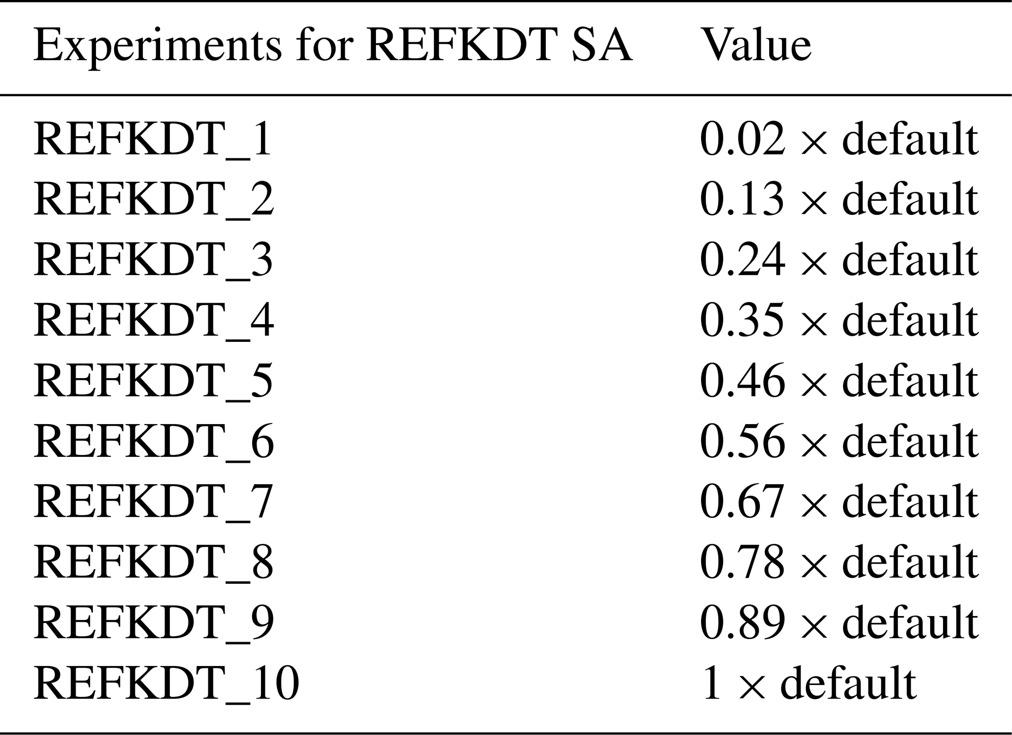
Note that the default is obtained from the WRF-Hydro GIS pre-processing toolkit. × indicates multiplication.

Sensitivity to the groundwater component

We investigate the sensitivity of groundwater components through two experiments by tuning the parameter GWBASEWCTRT, which involves two options in our study. One option creates a sink at the bottom of the soil column where water draining from the soil exits the system into this sink, while the other bypasses the bucket model, directly transferring all water draining from the bottom of the soil column into the channel. These two options are referred to as GWBASEWCTRT_Sink and GWBASEWCTRT_Passthrough in this study, respectively.

Sensitivity to lake–reservoir parameters

The Morris method (Morris, 1991) was employed to analyze the sensitivity of the seven lake–reservoir-related parameters, due to its low computational cost and ease of interpretation (Wei, 2013). This method is widely used for global sensitivity analysis in hydrological models, especially in computationally expensive models (Song et al., 2013; Wei, 2013). In the study, the sensitivity analysis was simultaneously conducted on the five lakes to reduce computational cost. In the Morris experiment, the eight main lake–reservoir-related parameters of the five lakes were normalized to a range of 0–1 by subtracting the minimum value and dividing by the maximum minus the minimum (Table 5). Based on the eight normalized values with a lower value of 0 and an upper value of 1, we generated all samples for Morris screening. The number of replications R, level p, and sample size N were set as 10, 4, and 90 (i.e., 90 parameter sets for 90 runs), respectively. For each sample, corresponding to a WRF-Hydro simulation, the eight parameters for each lake–reservoir system were inverse normalization. The other parameters were kept as their defaults. Two metrics were generated to examine the sensitivity: order of importance (u^∗ in Fig. 8) and dependencies with other parameters ($\mathit{\sigma }/u^{\ast }$ in Fig. 8). The u^∗ of a specific parameter with a higher value indicates greater sensitivity. The large value of $\mathit{\sigma }/u^{\ast }$ indicates stronger dependencies with other parameters.

Table 5 Sensitivity analysis (SA) experiments designed for MannN of the first five stream orders.

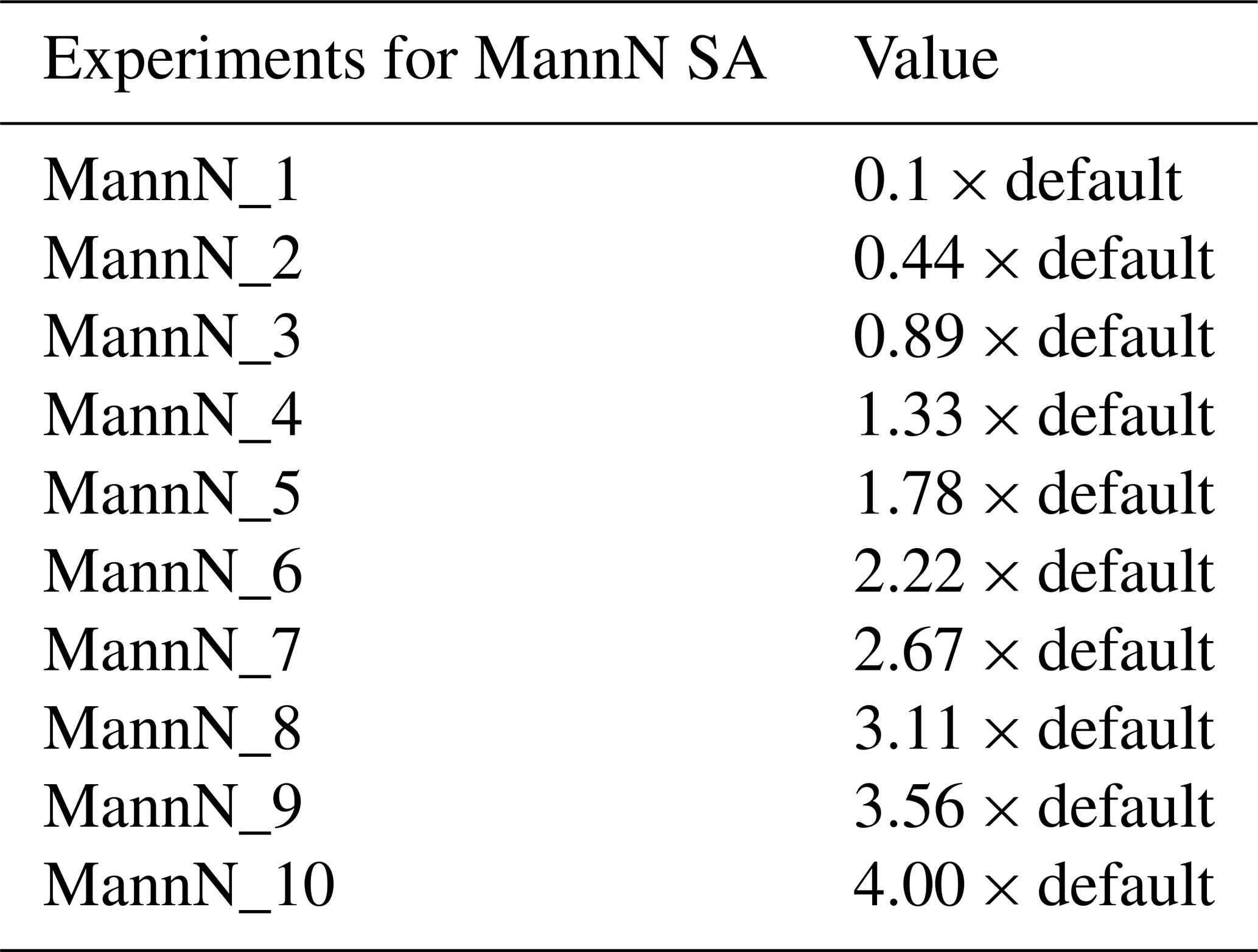
Note that the default is obtained from the WRF-Hydro GIS pre-processing toolkit. × indicates multiplication.

We also compared the sensitivity of the simulated discharge to lake–reservoir-related parameters across the five lakes. To conserve computational resources, the tests were based on the simulations from the calibration. For each test of parameters related to one lake, more than 30 simulations were conducted. Each simulation related to a given lake involves seven parameters (LkMxE, WeirE, OrificeE, WeirC, WeirL, OrificeC, and Dam_Length). In all simulations for a given lake, the values of these seven parameters varied synchronously, changing linearly from the minimum to the maximum, as shown in Table 6.

Table 6 Sensitivity analysis experiments designed for the eight lake–reservoir-related parameters.

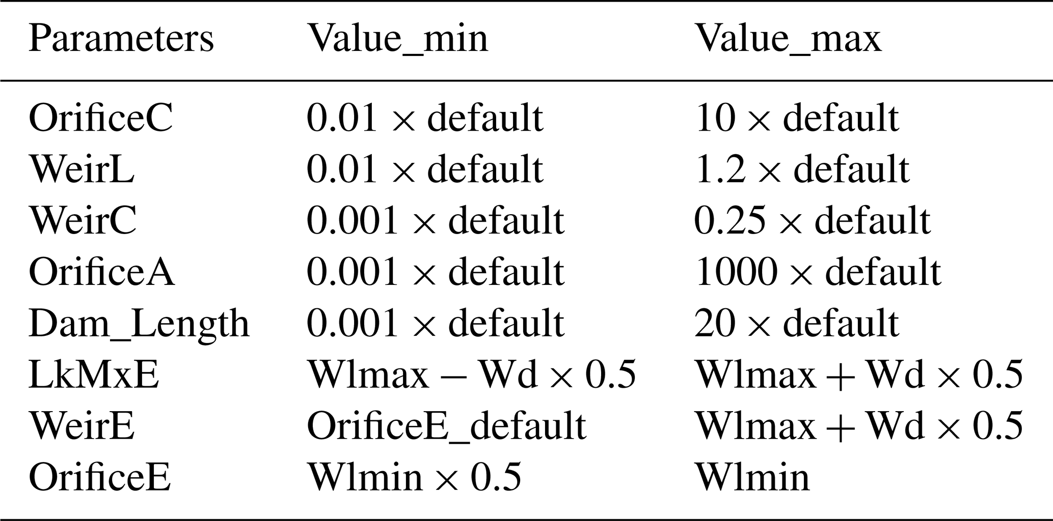
Note that Wlmax, Wlmin, Wd, and OrificeE_default indicate the max water level, min water level, water depth, and OrificeE default value, respectively. The default is obtained from the WRF-Hydro GIS pre-processing toolkit.

In the parameter setting, we make some rules to constrain three parameters (i.e., LkMxE, WeirE, and OrificeE) to make the simulation result reasonable: (1) LkMxE should be larger than both WeirE and OrificeE, and (2) OrificeE was suggested to be smaller than WeirE. To satisfy these constraints, OrificeE is set to be below the minimum water level, WeirE ranges from the OrificeE default value to the maximum water level plus half the water depth, and LkMxE changes from the maximum water level minus haft the depth to the maximum water level plus half the depth. Besides this, OrificeC and WeirC should be kept between 0 and 1, which should be a constant. The selection of maximum and minimum values, as well as the number of experiments, is flexible, as long as they are reasonable and produce realistic simulations.

3.2.3 Final calibration for WRF-Hydro modeling with the lake–reservoir module

Based on the sensitivity analysis, we developed a comprehensive calibration strategy for the WRF-Hydro system incorporating the lake–reservoir module. Building on the preliminary calibration (Sect. 3.2.1), we re-tuned the lake–reservoir-related parameter sets for the five lakes, respectively. Of the lake–reservoir parameter sets, each was calibrated sequentially from upstream to downstream, with more than 30 experimental iterations. Once the upstream lake was calibrated, its parameters were fixed as optimized and we proceeded to calibrate the parameters set for the next downstream lake. Subsequently, we focused on re-tuning REFKDT and MannN, each subjected to 30 experimental iterations. The parameter sets for each iteration were generated according to Sect. 3.2.2. Throughout this process, we achieved a well-calibrated lake-integrated WRF-Hydro model (LakeCal) with an optimal parameter set, determined by the best NSE value calculated over simulated discharge from January 2011 to December 2014 against the observations at Garissa station. Typically, we would use the same time series for discharge analysis as for the precipitation evaluation (2010–2014). However, since WRF-Hydro requires at least 1 year of spin-up, the discharge evaluation excludes the first year, focusing instead on the period from 2011 to 2014.

3.3 Peak flow, dry-season flow, and rainy-season flow

To measure modeling performance, we obtained the flow from the long rainy season of March–May (MAM), the short rainy season of October–December (OND), and the dry season of January–February (JF) and June–September (JJAS), as well as the peak flow. The maximum observed daily discharge at Garissa station over 2010–2014 occurred on 26 November 2011 (844 m³ s⁻¹) and is used as a peak flow case (Peak-Flow) for our evaluation. Since the model cannot capture the peak on the exact date, the simulated Peak-Flow was set as the largest daily discharge during the 21 d period centered around the observed Peak-Flow.

3.4 Evaluation of simulated precipitation from CPWRF

To assess whether the CPWRF has advantages over their driving forces (ERA5), added value (AV) proposed by Dosio et al. (2015) was applied, expressed as follows.

$$\begin{array}{}\text{(3)}& \mathrm{\text{AV}}={\displaystyle \frac{(X_{\text{ERA5}}-X_{\text{IMERG}}{)}^{\mathrm{2}}-(X_{\text{CPWRF}}-X_{\text{IMERG}}{)}^{\mathrm{2}}}{max\left(\right(X_{\text{ERA5}}-X_{\text{IMERG}}{)}^{\mathrm{2}},(X_{\text{CPWRF}}-X_{\text{IMERG}}{)}^{\mathrm{2}})}}\end{array}$$

X_ERA5, X_CPWRF, and X_IMERG indicate precipitation from the driving forces (ERA5), CPWRF simulation, and benchmark (IMERG), respectively. The added value (AV) from CPWRF is defined as the performance difference between itself and the driving forces for precipitation in a specific region and period. If the CPWRF adds value compared to the driving forces from ERA5, AV is positive, whereas a negative AV suggests no added value.

To fully evaluate the simulated precipitation by CPWRF, we also employed Taylor diagrams (Taylor, 2001), which present a concise statistical summary in terms of spatial correlation (indicated by the correlation coefficient) and spatial variance (indicated by the normalized standardized deviation). A higher spatial correlation and a spatial variance closer to 1 indicate better simulation skills.

3.5 Attribution of hydrological model improvement to convection-permitting WRF simulation and the lake–reservoir module

To assess the contributions of CPWRF simulations and the lake–reservoir module, we compared three models: (1) the calibrated WRF-Hydro model without the lake–reservoir module, driven by CPWRF output (LakeNan); (2) the well-calibrated WRF-Hydro model integrated with the lake–reservoir module, also driven by CPWRF output (LakeCal); and (3) the well-calibrated WRF-Hydro simulation with the lake–reservoir module, driven by ERA5 (LakeCal-ERA5). We calculated the NSE value of simulated discharge against observed data for each model. Next, we computed the NSE increment between LakeCal relative to LakeNan, representing improvements due to CPWRF precipitation, and the increment between LakeCal and LakeCal-ERA5, reflecting the influence of the lake–reservoir module. The ratio of the CPWRF precipitation-induced or lake–reservoir-module-induced NSE increment to the total increment is provided as the attribution of hydrological simulation improvements to the CPWRF simulations or the lake–reservoir module.

4 Results

4.1 WRF precipitation refinement

Using IMERG precipitation as a benchmark, we evaluated the performance of CPWRF precipitation at a 5 km resolution in the TRB, compared to the ERA5 reanalysis, which served as the forcing for our CPWRF simulation. This evaluation focused on seasonal precipitation averaged over 2010–2014 (Fig. 2) and daily precipitation distribution (Fig. 3). A Taylor diagram (Taylor, 2001), with spatial correlation (r, correlation coefficient) and spatial variance (normalized standardized deviation), is also applied for evaluation (Fig. S2 in the Supplement).

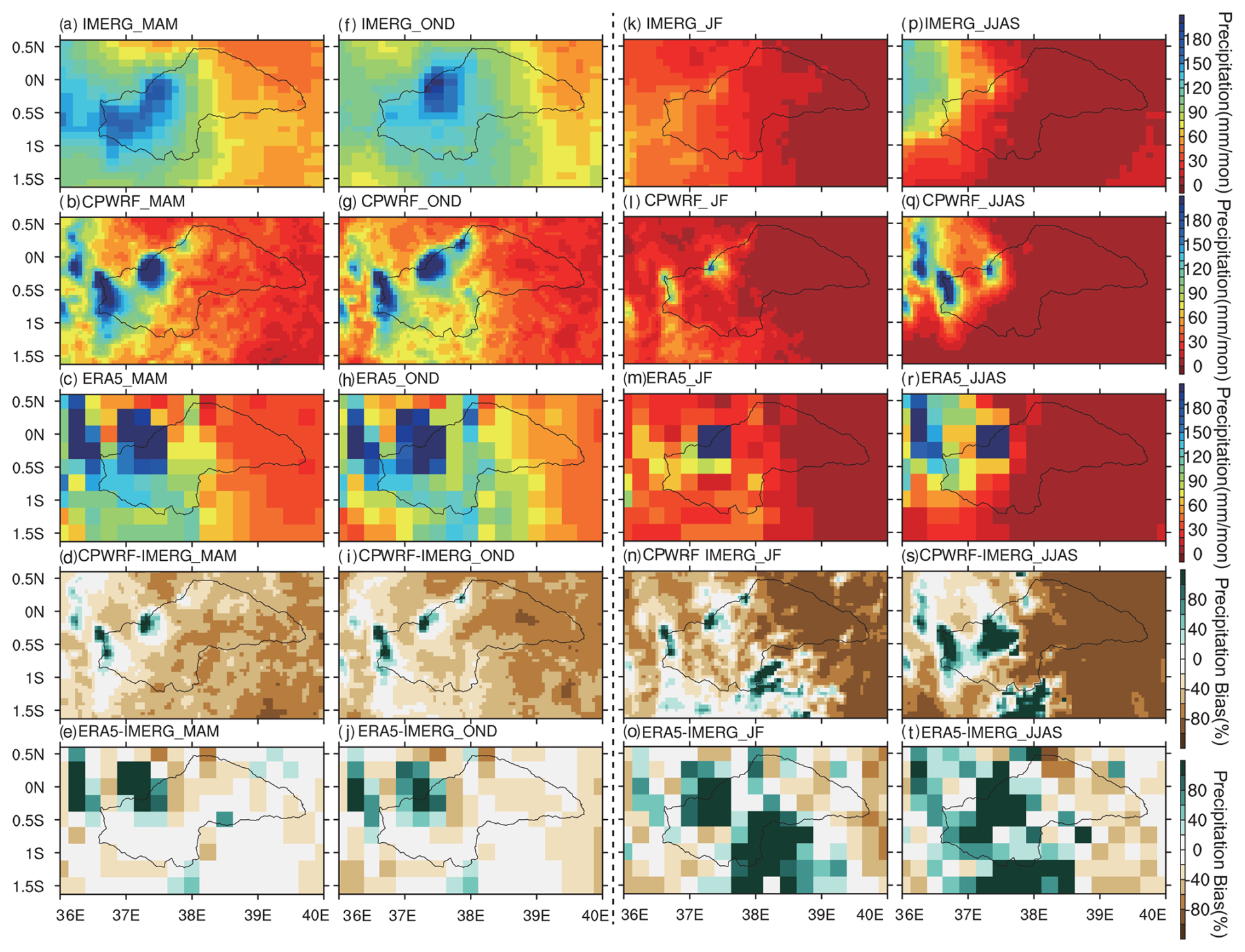
Figure 2 Seasonal precipitation of March–May (MAM; long rainy season, a–c), October–December (OND; short rainy season, f–h), January–February (JF; k–m), and June–August (JJAS; p–r) over the upper and middle stream of the Tana River basin (TRB), as well as its bias (d–e, i–j, n–o, s–t). Data from IMERG (a, f, k, p), WRF (b, g, i, q), and ERA5 (c, h, m, r). IMERG compared to the bias of CPWRF (d, i, n, s) and ERA5 (e, j, o, t). The seasonal precipitation (MAM, OND, JF, and JJAS) is calculated based on daily data (in March–May, October–December, January–February, and June–August) over 2010–2014. The gray polygon indicates the boundary of the upper and middle sections of the Tana River basin.

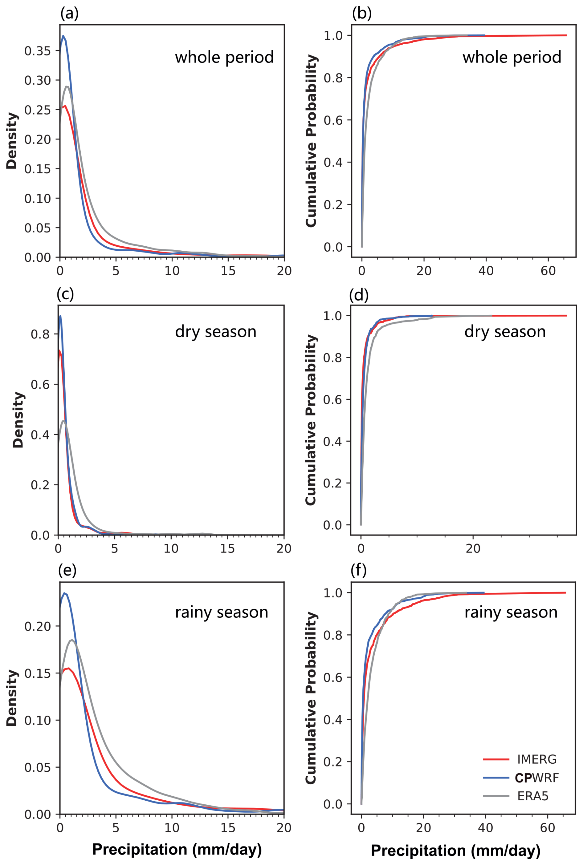
Figure 3 The distribution (a, c, e) and cumulative distribution (b, d, f) of daily precipitation from CPWRF (blue), ERA5 (gray), and IMERG (red, 2010–2014) over the whole period, dry season, and rainy season. Daily precipitation distribution over the whole period (a, b), dry season (c, d), and rainy season (e, f).

The CPWRF model captures the spatial pattern of precipitation and its seasonal variations over the TRB, as presented in IMERG (Fig. 2 and Table 7). The spatial distribution of the CPWRF simulation reveals that the precipitation is primarily concentrated in mountainous regions, such as Mount Kenya and the Aberdare Range, and surrounding areas (seen in Fig. 1b), with significantly less precipitation in the plain area (Fig. 2b, g, l, and q). The annual mean precipitation is approximately 1500 mm in the mountainous areas compared to less than 500 mm in the plain area (Table 7). During the rainy seasons (MAM and OND), total precipitation is 976 mm over the mountainous area and 327 mm over the plain area, in contrast to 417 and 33 mm during the dry season (JF and JJAS). This spatial and seasonal pattern is consistent with that in IMERG data (Fig. 2a, f, k, and p), indicating a distinct orographic and seasonal dominance.

Table 7 Seasonal and annual precipitation averaged over the mountainous (elevation >1600 mm) and plain (elevation <1600 mm) area.

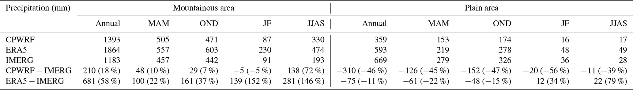
Note that precipitation from IMERG is the benchmark for evaluating the CPWRF simulation.

Compared to ERA5, CPWRF precipitation generally shows better performance, indicated by the Taylor diagram (Fig. S1e and f in the Supplement) in terms of spatial correlation (correlation coefficient) and spatial variance (normalized standardized deviation), although the advantage is not obvious. The median correlation coefficient of CPWRF precipitation against IMERG is 0.80, higher than ERA5's value of 0.66 (Fig. S1e). Similarly, the median normalized standardized deviation of CPWRF precipitation is 1.1, closer to 1 compared to ERA5's value of 1.7 (Fig. S1f). The improved performance of CPWRF is also evident from the model-data bias comparison. The CPWRF simulation shows a smaller area with large biases (exceeding 60 %) compared to ERA5. During MAM, OND, JF, and JJAS, the areas with large biases are 618.2 km² (1.9 %), 711.0 km² (2.2 %), 680.0 km² (2.1 %), and 3431.0 km² (10.4 %), respectively. In contrast, ERA5 shows corresponding areas of 1545.5 km² (4.7 %), 1545.5 km² (4.7 %), 10818.3 km² (32.9 %), and 8500.1 km² (25.9 %), respectively.

Spatially, the superior performance of CPWRF precipitation compared to ERA5 merges in the mountainous regions, mainly over Mount Kenya and its surroundings, as demonstrated by the spatial distribution of the model-data bias (Fig. 2d–e, i–j, n–o, and s–t) and AV (Fig. S2) result. Specifically, the model-data bias from CPWRF is 210 mm (18 %) per year over the mountainous areas, whereas ERA5 shows a bias of 681 mm (58 %) (Table 7). Additionally, over the mountainous areas, CPWRF adds value to ERA5 (Fig. S2a–e), with a positive AV of 0.14 averaged across the four seasons and this area. Such improvement over the mountainous areas is more pronounced in the JF season. The model-data bias in the JF season is −5 mm (−5 %) from CPWRF and 139 mm (152 %) from ERA5. In contrast, during MAM, OND, and JJAS, the bias is 29 mm (7 %), 48 mm (10 %), and 138 mm (72 %) from CPWRF with values of 161 mm (37 %), 100 mm (22 %), and 281 mm (146 %) from ERA5. The improvement over the mountainous areas during the JF season is highlighted in the Taylor diagram (Fig. S1c). The spatial correlation or normalized standardized deviation, calculated over the JF-averaged precipitation in the mountainous areas, is 0.56 or 2.18 for CPWRF, in contrast with −0.14 or 5.46 for ERA5.

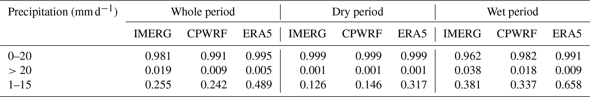
Also, the probability distribution of regionally averaged daily precipitation from the CPWRF result exhibits better alignment with the benchmark than from ERA5 (Fig. 3). The CPWRF aligns more closely with IMERG for both small (0–20 mm d⁻¹) and extreme (>20 mm d⁻¹) rainfall events compared to ERA5, as shown in Fig. 3 and Table 8. The cumulative probability of the small (or extreme) rainfall is 0.991 (0.009) from CPWRF and 0.981 (0.019) from IMERG, whereas it is 0.995 (0.005) from ERA5. Among these, the better alignment of the probability of light rainfall (1–15 mm d⁻¹) between CPWRF and IMERG is pronounced (Fig. 3 and Table 8). The probability of light rainfall is 0.255 from CPWRF and 0.242 from IMERG, whereas it is 0.489 from ERA5. Consistently, CPWRF adds value to ERA5 over the probability of light rainfall (Fig. S2f–k), with a positive AV of 0.21 averaged across the basin during the four seasons. The better alignment of light rainfall from CPWRF than ERA5 is particularly evident during the dry season (Fig. 3). The probability of 1–15 mm d⁻¹ events during the dry season from CPWRF is 0.15 and 0.13 from IMERG, whereas it is 0.32 from ERA5.

Table 8 Cumulative distribution of daily precipitation regionally averaged over the TRB, from the CPWRF simulation, IMERG, and ERA5.

4.2 WRF-Hydro model optimization with the lake–reservoir module

4.2.1 A preliminary investigation of the lake–reservoir impact on discharge

To assess the impact of the lake–reservoir module on hydrological simulation, we compared simulated discharges from different WRF-Hydro modeling experiments against the observations. These experiments included WRF-Hydro with the lake–reservoir module (LakeRaw) and without it (LakeNan), as shown in Fig. 4. The evaluation results (including the Kling–Gupta efficiency, KGE; bias; r²; and NSE) from all these experiments are presented in Table S2 in the Supplement. The WRF-Hydro model with the lake–reservoir module (LakeRaw) improves discharge simulation compared with that without it (LakeNan), even without model calibration. LakeRaw achieved an NSE of 0.01 and a bias of 40 %, compared to −1.09 and −53 % from the LakeNan. The inclusion of the lake–reservoir module addresses the underestimation of dry-season flows. However, the lake–reservoir module (in the LakeRaw) tends to induce overestimation, particularly during February–March and August–September, contributing approximately 81 % of the annual average dry-season flows. This overestimation in LakeRaw is likely due to uncalibrated parameters, including spin-up time, the hydrological parameters, the groundwater component, and the lake–reservoir-related parameters. The hydrological parameters, groundwater component, and lake–reservoir-related parameters need to be further adjusted when the lake–reservoir system is included in WRF-Hydro system. To enhance the performance of WRF-Hydro modeling with the lake–reservoir module, the sensitivity and optimization potential of these parameters were investigated.

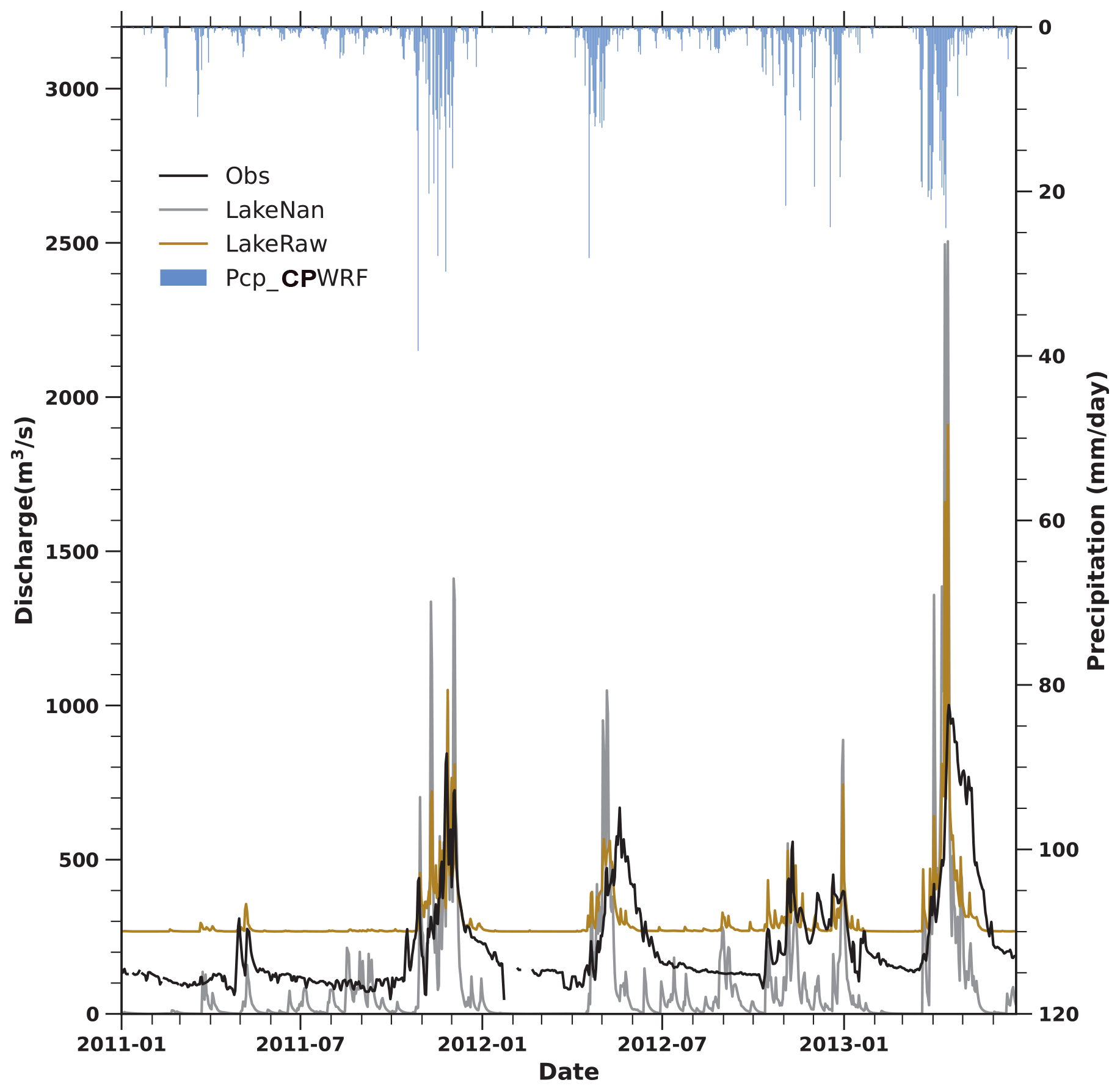
Figure 4 The simulated daily discharges from WRF-Hydro modeling without the lake–reservoir module (LakeNan, the gray line) and with the lake–reservoir module using parameters from LakeNan (LakeRaw, the brown line) against the observations (the black line), as well as the daily precipitation from the CPWRF simulation (Pcp_CPWRF, the blue bar).

4.2.2 Spin-up time

In the LakeRaw simulation, the spin-up sensitivity is highlighted by the discharge during 2011–2014 from the 17 spin-up experiments (Fig. 5 and Table 3). The simulated discharge at the Garissa station, on the first day (26 November 2011, the observed Peak-Flow day), differs between almost every experiment. The simulated Peak-Flow at the Garissa station decreases as the spin-up time gets shorter, which reaches 485 m³ s⁻¹ in the 12-year spin-up experiment (“12y spin-up” in Fig. 5a) but only 211 m³ s⁻¹ in the 1 d spin-up experiment (“1d spin-up”) from the LakeRaw simulation. The reduction in first-day discharge suggested that insufficient spin-up time results in more runoff being allocated to soil moisture and groundwater, which have not yet reached equilibrium. In general, Peak-Flow runoff increases slightly with longer spin-up times, up to the 6-year spin-up (Fig. 5b). Also, the average discharge shows distinct sensitivity to different spin-up times (Fig. 5d and e). The average discharge at Garissa over the entire period, as well as during the rainy and dry seasons from 2011–2014, shifted from an underestimation of −49 %, −44 %, and −52 % in the 1 d spin-up experiment to an overestimation of 21 %, 54 %, and 7 % in the 12-year spin-up experiment. The LakeRaw simulation generally needs approximately 4 years for the annual discharge at Garissa to stabilize (Fig. 5d and e).

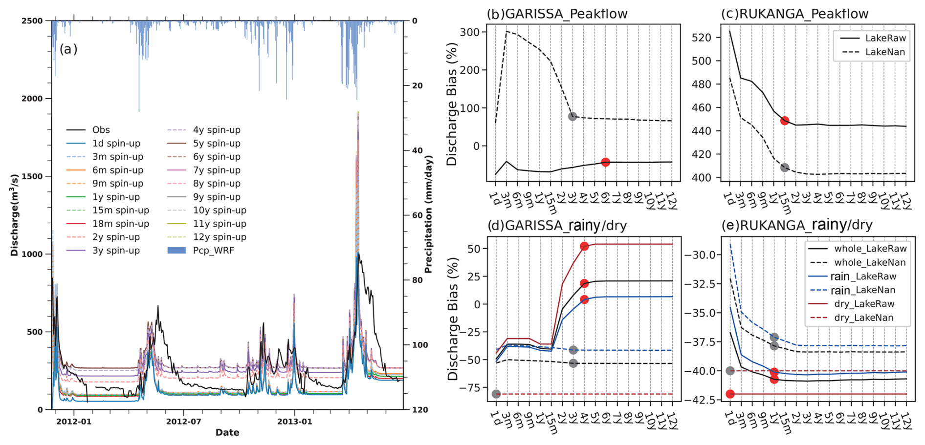
Figure 5 Sensitivity analysis results from the 17 different spin-up experiments. (a) Simulated discharge with spin-ups (the colored lines) ranging from 1 d (1d spin-up) to 12 years (12y spin-up) against the observation (Obs; the black line) for the LakeRaw module. The blue bars indicate the daily precipitation from the convection-permitting WRF simulation. (b–e) Model-data bias of discharge at Garissa (b, d) and Rukanga (c, e), with an increase in spin-up time, which is from LakeNan (WRF-Hydro simulation with the lake–reservoir module, solid line) or LakeRaw (WRF-Hydro simulation without the lake–reservoir module using parameters from LakeNan, dashed line) over the entire year (black line), rainy season (March–May and October–December, blue line), and dry season (January–February and June–September, red line). The dot indicates the spin-up time required for LakeRaw (red) or LakeNan (gray) to reach equilibrium. Therein, Peak-Flow (Peakflow) is the largest daily discharge over the 21 d centered around the observed peak (largest observed daily discharge over 2011–2014).

The initial time differs spatially, with shorter spin-up in the upstream area compared to the downstream area. In the LakeNan simulation, the initialization time of discharge metrics (i.e., Peak-Flow, average discharge, rainy-season flow, and dry-season flow) at Rukanga station upstream is less than 2 years, while at the downstream Garissa, it can extend to 3 years. The longer spin-up in the downstream area might be ascribed to the larger drainage area, which requires a longer convergence time compared to the upstream. The prolongation of spin-up time is more distinct in the simulation with the lake–reservoir module than in the one without it. In the LakeRaw simulation, the initialization time for discharge metrics upstream (Rukanga station) remains under 2 years, while the initialization time for Peak-Flow downstream (Garissa station) extends to 6 years. This significant prolongation of spin-up time indicates the lake–reservoir impact.

The lake–reservoir module seems to prolong the required spin-up time for the downstream area (Fig. 5b). In addition to Peak-Flow, the spin-up time for the whole-period, dry-season, and rainy-season flow is prolonged to 4 years in the LakeRaw simulation, compared to 3, 0, and 3 years, respectively, in the LakeNan simulation. The larger spin-up difference in dry-season discharges between the LakeRaw (3 years) and LakeNan (0 years) simulations demonstrates a greater sensitivity of the dry season to the lake–reservoir module, compared to the rainy season.

The water levels from the lake–reservoir-integrated model show a consistent spin-up period of 4 years across nearly all five lakes for the entire period, as well as during both the rainy and dry seasons (Fig. S2). Although Kiambere (one of the five lakes) exhibits a spin-up period of 3 years during the rainy season (Fig. S2e), it can be considered nearly 4 years due to the uncertainty in determining the spin-up time required for the stabilization of specific variables. Since the lakes are interconnected, the stabilization time is governed by the longest spin-up period. This may result in nearly the same initialization time for all five lakes (Table 1).

4.2.3 Sensitivity analysis from hydrological parameters

The MannN parameter exhibits a substantial impact on the peak flow, with lower values corresponding to higher discharge peaks (Fig. 6a and Table S3 in the Supplement). As the MannN scale decreases from 4 to 0.1, the average discharge at Garissa increases from 294 to 297 m³ s⁻¹ and Peak-Flow increases from 975 to 1309 m³ s⁻¹. In addition, the smaller MannN value delays the arrival of peak flows, shifting the Peak-Flow date from 6 December 2011 to 2 December 2011 – an advance of 4 d – as MannN decreases from 4 to 0.1. This effect is due to MannN representing channel roughness, which influences both streamflow transit time and volume.

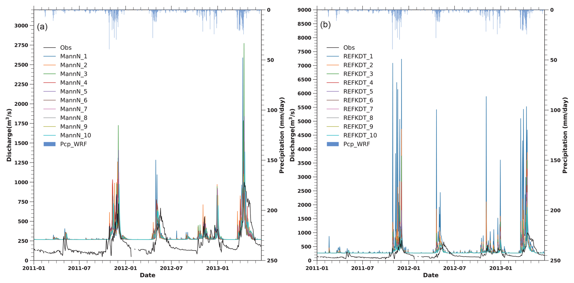
Figure 6 The simulated WRF-Hydro discharge at Garissa from January 2011 to June 2013 from the Manning roughness parameter (MannN) and runoff infiltration coefficients (REFKDT) sensitivity tests against the observation (Obs). The MannN (or REFKDT) test consists of 10 simulations, with the MannN (or REFKDT) ranging from a scale of nearly 0 (or 0.02) in the MannN_1 (or REFKDT_1) experiment to a scale of 4 (or 1) in MannN_10 (or REFKDT_10) with nearly equal intervals in between. Precipitation from the WRF simulation (Pcp_CPWRF) is shown on the top.

Similarly, the REFKDT parameter also significantly impacts peak discharge in response to heavy rain. An increase in REFKDT generally results in decreased discharge (Fig. 6b and Table S4 in the Supplement). Specifically, when the REFKDT scaling factor changes from 0.02 (REFKDT equals 0.1) to 1 (REFKDT equals 5), Peak-Flow decreases from 7229 to 1092 m³ s⁻¹. In the WRF-Hydro modeling system, the REFKDT parameter governs surface infiltration by partitioning runoff into the surface and subsurface components (Schaake et al., 1996). A higher REFKDT value allows more water into the subsurface, thereby reducing surface runoff and peak discharge.

However, both MannN and REFKDT have minimal effects on alleviating the underestimation of dry-season flow shown in the above WRF-Hydro simulations with the lake–reservoir module (LakeRaw) (Fig. 4). The dry-season flow remains largely unchanged despite variations in these two parameters.

4.2.4 Sensitivity analysis from groundwater components

Overall, adjusting groundwater component options could slightly alleviate the overestimation of dry-season flow (Fig. 7 and Table S5 in the Supplement). The dry-season flows from the two experiments have large overestimations with a considerable bias of 122 (81 %) and 161 (107 %) m³ s⁻¹, respectively. However, in the GWBASESWCRT_Passthrough experiment, the simulated discharge fluctuation aligns better with the observation, compared to the GWBASESWCRT_Sink experiment. The determination coefficients (r²) of the simulated discharge against the observation are 0.56 and 0.33 in the GWBASESWCRT_Passthrough and GWBASESWCRT_Sink experiments, respectively. Besides, the discrepancies in the waveform in the GWBASESWCRT_Sink experiment cause an earlier prediction of flood retreat. Given the relatively better performance of the GWBASESWCRT_Passthrough experiment, we selected the pass-through bucket module for the subsequent sensitivity analysis and calibration experiment.

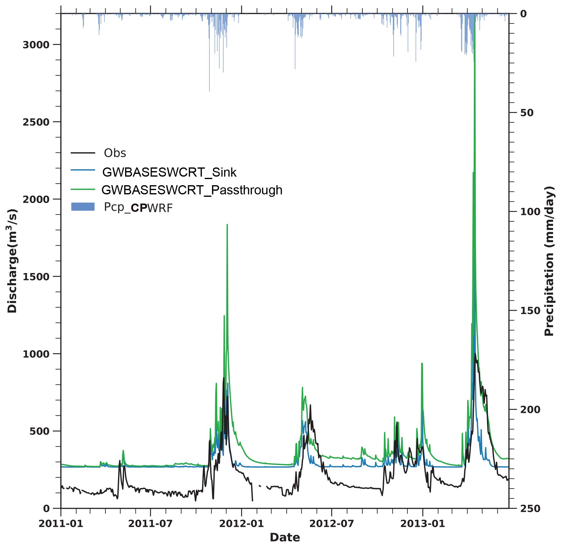
Figure 7 The discharge evolution of the two experiments and the observation. One experiment creates a sink on the bottom of the soil column, where water drains out of the system (GWBASESWCRT_Sink), while the other bypasses the bucket model and directly transfers all flow from the bottom of the soil column into the channel (GWBASESWCRT_Passthrough). Precipitation from the CPWRF simulation (Pcp_CPWRF) is shown on the top.

4.2.5 Sensitivity analysis from lake–reservoir-related parameters

From the results of the Morris method (Fig. 8 and Table S6), lake–reservoir-related parameters (i.e., LkMxE, WeirE, WeirC WeirL, OrificeA, OrificeC, and OrificeE) show a clear influence on the discharge at Garissa. The overestimation of discharge was reduced in the best-performing simulation with the largest NSE (represented by the red line in Fig. 8a). Among the eight lake–reservoir-related parameters, WeirE is the most sensitive, as indicated by its top sensitivity ranking (Fig. 8b). Modifying WeirE from its maximum (maximum water level plus half the water depth) to its minimum (the default orifice elevation) in the LakeRaw model with other parameters set at their defaults (Table S6) resulted in the average discharge varying from 311 to 38 m³ s⁻¹, with the model-data bias varying from 19 % to less than −85 %. This sensitivity is particularly pronounced during the dry season, with a bias difference of 244 m³ s⁻¹ on average during 2011–2014, corresponding to −163 % of the observed values. This finding highlights that adjusting lake–reservoir-related parameters can significantly reduce the overestimation of dry-season flow, showing promise for improving the model's overall performance. Notably, the eight parameters exhibit distinct interdependence, as indicated by the large value of $\mathit{\sigma }/u$ (>0.5) (Fig. 8c), suggesting that parameter optimization should be conducted globally rather than locally.

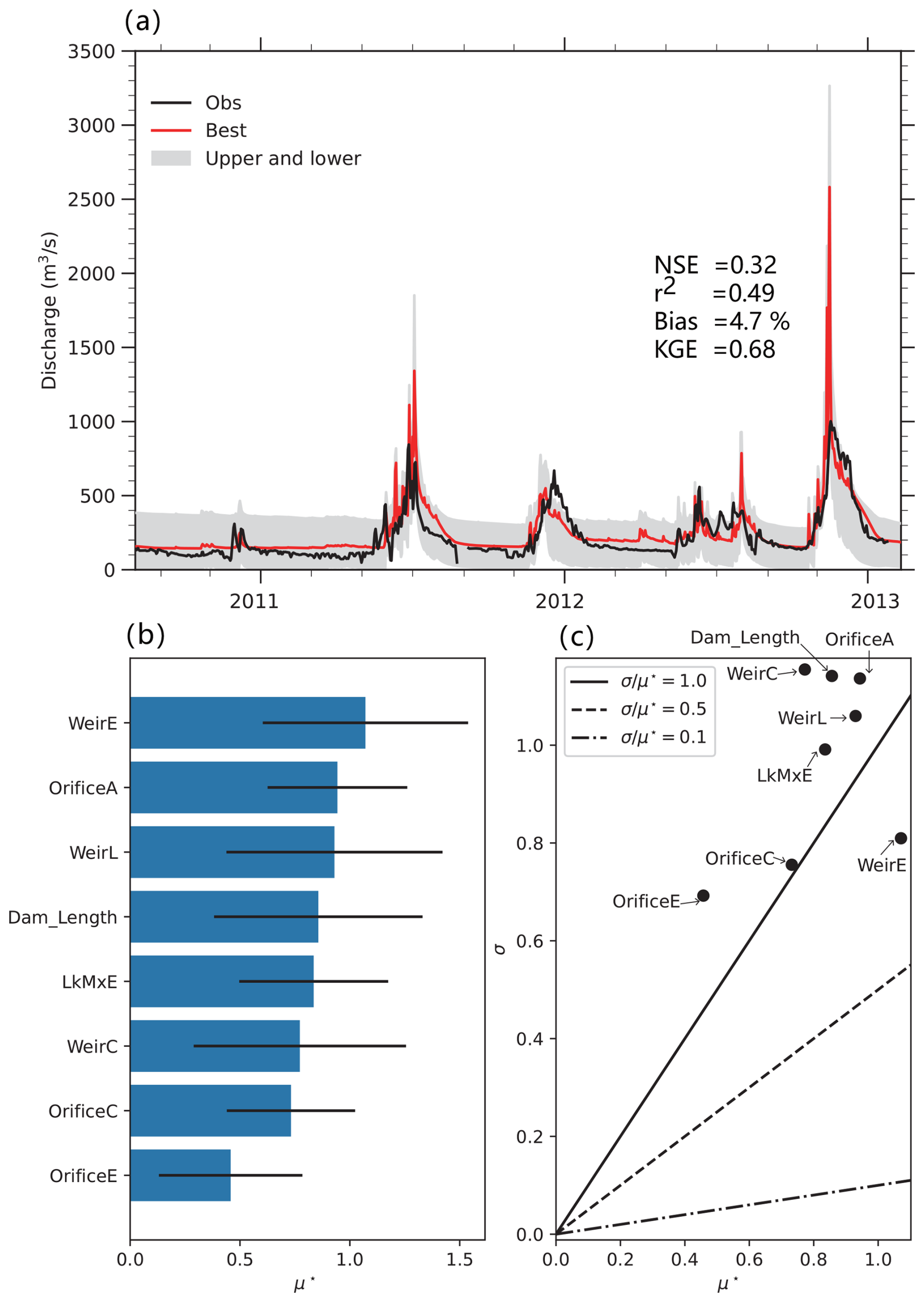
Figure 8 The Morris results, including simulated discharge from 90 experiments against the observation (a), the sensitivity ranking of parameters (b), and their interdependence (c). The Nash–Sutcliffe efficiency (NSE), the coefficient of determination (r²), bias (unit: %), and the Kling–Gupta efficiency (KGE) are calculated based on the best-simulated discharge at Garissa (red line, which corresponds to the largest NSE) against the observations. u^∗ donates the sensitivity of a given parameter, with a higher value indicating greater sensitivity. The large value of $\mathit{\sigma }/u^{\ast }$ indicates stronger dependencies with other parameters.

Although adjusting lake–reservoir-related parameters can alleviate the overestimation of dry-season flow, it induces a new issue: a simultaneous decrease in rainy-season discharge, leading to its underestimation. Modifying WeirE in the LakeRaw model (keeping other parameters at their default settings) results in a shift in rainy-season flow from a wet bias (52 m³ s⁻¹, 19 %) to a dry bias (−197 m³ s⁻¹, −71 %). This bias change is also observed in Peak-Flow, which varied from an overestimation of 165 m³ s⁻¹ (20 %) to an underestimation of −127 m³ s⁻¹ (−16 %). Fortunately, the rainy-season flow underestimation could be re-adjusted by REFKDT or MannN, as well as Peak-Flow.

Lakes with larger surface areas appear to play a dominant role in affecting discharge biases, as shown in Fig. S4 in the Supplement. Adjusting parameters of larger lakes, such as Masinga, Kamburu, and Kiambere, leads to greater variations, reflected in larger standard deviations, compared to smaller lakes like Gitaru and Kindaruma. Among the five lakes, Masinga (the largest, with an area of 111.6 km²) exhibits the most significant impact on discharge, with standard deviations of 21 % for Peak-Flow, 23.7 % for average discharge, 19 % for rainy-season flow, and 34 % for dry-season flow. In contrast, Kindaruma (the smallest, with an area of 2.1 km²) exhibits the least impact on discharge, with near-zero standard deviations (0.1 %, 0.3 %, 0.2 %, and 0.6 %, respectively).

4.2.6 The optimized results of WRF-Hydro modeling with the lake–reservoir module

Based on the sensitivity analysis result, we conducted a calibration involving the parameters outlined above, and the results are shown in Fig. 9 and Table S2. Calibration of the WRF-hydro modeling system with the lake–reservoir module greatly improves the simulation of river discharges in the TRB. The simulated discharge from LakeCal with an NSE of 0.57 and a bias of 9 % is more consistent with the observed flow process, compared to LakeRaw with an NSE of 0.01 and a bias of 40 %. The significant overestimation of discharge in the LakeRaw (Sect. 4.2.1) model was notably reduced through the calibration of the lake–reservoir module, although a slight overestimation remains.

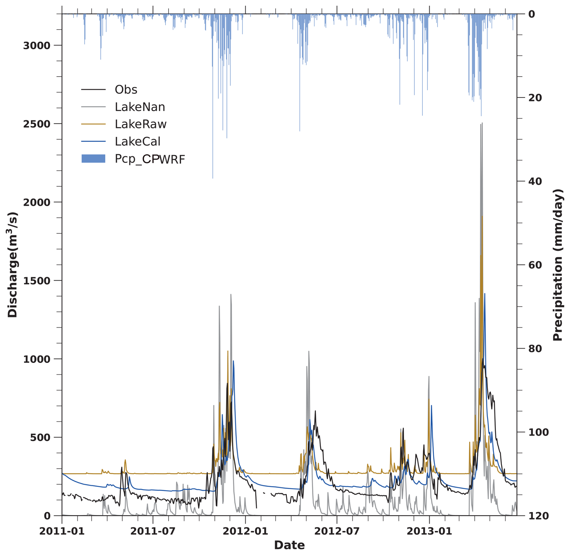
Figure 9 The simulated discharges from three WRF-Hydro simulations against the observation. The three simulations include WRF-Hydro without the lake–reservoir module (LakeNan in gray), WRF-Hydro with the lake–reservoir module based on parameters from LakeNan (LakeRaw, in brown), and well-calibrated WRF-Hydro with the lake–reservoir module (LakeCal, in blue). Precipitation from the CPWRF simulation (Pcp_CPWRF) is shown on the top.

Notably, the modeling performance of the WRF-Hydro simulation with the lake–reservoir module (LakeCal) is much better than that without the lake–reservoir module (LakeNan). The NSE and bias are −1.09 and −53 % in the LakeNan simulation, compared to 0.57 and 9 % in the LakeCal simulation. The improvement is particularly evident during dry-season flow and the Peak-Flow simulation, despite a slight overestimation of dry-season flow. The calibration of the WRF-Hydro modeling system with the lake–reservoir module corrects the overestimation of dry-season flow by 71 m³ s⁻¹, reducing the dry-season flow from 271 m³ s⁻¹(with a bias of 81 %) to 200.1 m³ s⁻¹ (with a bias of 34 %). Besides this, the deviation in Peak-Flow, indicated by a bias of 174 % (144 m³ s⁻¹), decreased in LakeCal to a bias of 24 % (206 m³ s⁻¹) in LakeRaw. Consistently, the overestimation of the average discharge in the rainy-season flow was reduced, with the bias changing from 22 % to −2 %. Due to this improvement in dry-season flow, the Peak-Flow simulation, and rainy-season flow, LakeCal better captures seasonal variation than the other two models. The r² is 0.75 in the LakeCal model, calculated over the simulated monthly discharge against the observation, compared to 0.66 in the LakeNan simulation. Furthermore, LakeCal could better capture the hydrograph shape during the rise and recession of floods, as indicated by the improved r² of 0.59, compared to 0.30 in LakeNan and 0.33 in LakeRaw. For example, during the MAM period in 2012 and 2013, the simulated onset and recession times of flooding by LakeCal were closer to the observation than those from the LakeRaw and LakeNan. The earlier estimation of flood onset times in LakeRaw was significantly alleviated in LakeCal. The better fit of the simulated discharge against the observation during flood rising and falling times in the WRF-Hydro system with the lake–reservoir module indicates a promising ability to accurately forecast floods.

5 Discussion

5.1 Attribution of hydrological simulation enhancement

The above skilled WRF-Hydro simulation of LakeCal (Fig. 9) could be attributed to the integration of the CPWRF simulation and the inclusion of the lake–reservoir module. To quantitatively assess the contributions from the CPWRF simulation and lake–reservoir module to discharge performance, we compared three models (LakeNan, LakeCal, and LakeCal-ERA5), and the results are presented in Figs. 9 and 10 and Table S2.

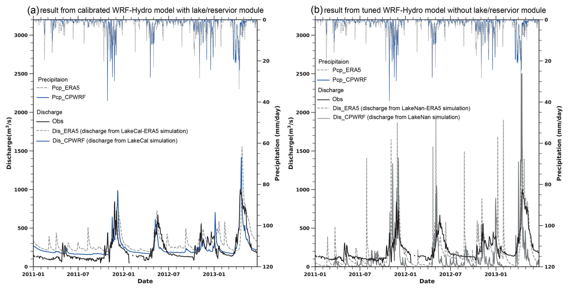
Figure 10 Precipitation from CPWRF (Pcp_CPWRF, solid line on the top) and ERA5 (Pcp_ERA5, dashed line on the top), as well as the simulated daily discharge evolution from WRF-Hydro driven by CPWRF precipitation (Dis_CPWRF, solid line on the bottom, colored blue in a and gray in b) and ERA5 precipitation (Dis_ERA5, dashed line on the bottom in both a and b) against the observation (dashed black line). Results from the calibrated WRF-Hydro model with (a) and without (b) the lake–reservoir model. LakeCal-ERA5 or LakeCal indicates the well-calibrated lake–reservoir-integrated WRF-Hydro simulation driven by ERA5 data or CPWRF output, while LakeNan-ERA5 or LakeNan indicates WRF-Hydro simulation without the lake–reservoir module driven by ERA5 data or CPWRF output.

The well-calibrated lake–reservoir-integrated model forced by CPWRF output (LakeCal) outperforms both the no-lake–reservoir model driven by CPWRF output (LakeNan) and the lake–reservoir-integrated model forced by ERA5 (LakeCal-ERA5). Comparing LakeCal to LakeCal-ERA5, the refined precipitation from CPWRF notably enhances the WRF-Hydro modeling performance, particularly in reducing the false peak simulation (Fig. 10a). The simulation skill indicated by NSE rises from 0.04 (LakeCal-ERA5) to 0.57 (the LakeCal) (Table S2), resulting in an NSE increase of 0.53. Comparing the LakeCal to LakeNan, the inclusion of the lake–reservoir module significantly improves the WRF-Hydro performance, distinct in alleviating the underestimation of the dry-season flow and the overestimation of the peak flow. The NSE rises from −1.10 (LakeNan) to 0.57 (LakeCal), leading to an NSE increase of 1.67. Dividing the total increases in NSE, improvements in hydrological simulation could be attributed as follows: 24 % (an NSE increase of 0.53) to the precipitation simulated by CPWRF and 76 % (an NSE increase of 1.67) to the inclusion of the lake–reservoir module.

5.2 Hydrological modeling improvement from CPWRF precipitation

Dynamic downscaling at convection-permitting resolution allows for a more accurate representation of precipitation processes. The CPWRF simulation enhances local (e.g., mesoscale) processes and interactions between local and large scales, especially over complex terrain (Kendon et al., 2021; Guevara Luna et al., 2020; Schmidli et al., 2006; Schumacher et al., 2020; Li et al., 2020). As a result, CPWRF potentially contributes to improving precipitation simulation in our study (Sect. 4.1), especially reducing bias in seasonal precipitation over mountainous areas and the probability of light rainfall (1–15 mm d⁻¹) in the dry season compared to ERA5 (Fig. 3 and Table 8).

The improvement in the seasonal precipitation over mountainous regions and rainfall probability can be supported by the spatial distribution of the added value (AV) in seasonal precipitation with respect to the driving forces (Fig. S2). The CPWRF simulation adds consistent value to ERA5 over the mountainous areas across all four seasons (MAM, OND, JF, and JJAS). The area with positive AV is mainly over Mount Kenya and its surrounding areas, with the positive AV being particularly distinct during the dry season. CPWRF also adds value to ERA5 regarding the probability of light rainfall (Fig. S2f–k), as demonstrated in Sect. 4.1. The basin-averaged AV of CPWRF over the probability of light precipitation events are 0.32, 0.26, 0.30, and 0.07 in MAM, OND, JF, and JJAS, respectively. The positive AV of CPWRF with respect to ERA5 over the extreme rainfall probability also concentrates around Mount Kenya consistently across all four seasons (Fig. S2l–p). Previous studies (Giorgi et al., 2022) have demonstrated that the added value of CPWRF simulations is influenced by various factors, including the timescale, variables, regions, and uncertainty in the benchmark. Therefore, further in-depth research is required for a more reliable AV assessment.

Due to the precipitation improvement from WRF, hydrological simulation with CPWRF precipitation as a driving force (LakeCal) showed significant improvements compared to simulations driven by ERA5 (LakeCal-ERA5) (Fig. 10a). These improvements are particularly notable in reducing false peak simulations, likely due to the reduction in the overestimation of the probability of light rainfall. The enhancement in the peak flow simulation is also observed in the WRF-Hydro model without the lake–reservoir module (Fig. 10b).

5.3 Hydrological modeling improvement from the lake–reservoir module

The lake–reservoir module is crucial for improving hydrological simulations over the TRB in East Africa. Several factors could contribute to overestimation issues presented in the LakeRaw simulation, even with adequate spin-up time, such as the groundwater component, key hydrological parameters, and lake–reservoir-related parameters. Despite some adjustments, the groundwater component (Sect. 4.2.4) and key hydrological parameters (Sect. 4.2.3) have a limited ability to alleviate the overestimation of dry-season flow in the lake–reservoir-integrated WRF-Hydro simulation without calibration (LakeRaw). In contrast, tuning lake–reservoir-related parameters could significantly influence downstream discharge (Sect. 4.2.6). This underscores the critical role of the lake–reservoir module in enhancing hydrological simulations in data-scarce regions that contain lakes or reservoirs.

Lakes and reservoirs play a crucial regulatory role, storing water during the rainy season (especially the peak flow period) and releasing water during the dry season (Zajac et al., 2017; Hanasaki et al., 2006). In our study, hydrological simulations without the lake–reservoir module (LakeNan) in the TRB, including five lakes, show significant underestimation (−78 %) in dry-season flow and overestimation (24 %) in Peak-Flow. The underestimation of dry-season flow and overestimation of Peak-Flow are well-documented issues in East Africa, as noted by Arnault et al. (2023). Previous studies demonstrated that enhancing reservoir hydrological processes can improve simulation accuracy (Hanasaki et al., 2006; Lehner et al., 2011) for basins with reservoirs or lakes. Our results confirm that the well-calibrated lake–reservoir-integrated WRF-Hydro system significantly reduces the underestimation of dry-season flow and overestimation of peak flow. The lake–reservoir module helps to adjust the dry-season flow bias from −78 % in the LakeNan simulation to 34 % in LakeCal, despite some remaining positive bias. The Peak-Flow bias in the lake–reservoir simulation decreased to 17 %, compared to a value of 24 % in the LakeNan simulation.

5.4 Uncertainties

Although the CPWRF simulation shows improved skill, evident in seasonal precipitation around Mount Kenya and the probability of light rainfall during the dry season, it is notable that CPWRF still displays uncertainties. This uncertainty involves wet biases in rainy seasons and dry biases in dry seasons (Fig. 2 and Table 7), as well as the overestimation of the probability of little rainfall (0–20 mm d⁻¹) and the underestimation of the probability of extreme rainfall (>20 mm d⁻¹) (Fig. 5 and Table 8). Although seasonal precipitation simulation from CPWRF exhibits an improvement in mountainous areas compared to ERA5, it is slightly degraded in the plain areas (Table S1 in the Supplement). The uncertainty might come from the driving data of ERA5, which could be observed with the same bias as the CPWRF result. Good-quality forcing drivers could be further used to improve the precipitation simulation in future work. Besides this, the benchmark (IMERG) in the data-scarce area presents challenges for precipitation evaluation. The uncertainty from IMERG precipitation over East Africa (Dezfuli et al., 2017) may complicate precipitation evaluation. In our study, the CPWRF simulation shows an underestimation of extreme precipitation (i.e., 90th–100th quantiles) against IMERG (Fig. 5b and f), while the simulated discharge from LakeCal, driven by CPWRF precipitation, does not exhibit the expected underestimation of extreme flow when compared to observations (Fig. 10b). The absence of the underestimation of extreme flow suggests IMERG may overestimate extreme precipitation compared to its actual representation. The overestimation of IMERG precipitation in Africa has been demonstrated in previous research (Maranan et al., 2020; Dezfuli et al., 2017), which could create the illusion of underestimation from WRF. Such erroneous underestimation of extreme precipitation from CPWRF was also indicated by the general overestimation of extreme flow in the LakeCal simulation (Fig. 10a and b). Therefore, we believe that the potential advantages of the CPWRF simulation are likely greater than what we have demonstrated by our result. Future work could benefit from incorporating more reliable observational data to enhance precipitation evaluation.

Different metrics (r, bias, and normalized standardized deviation) were used to provide a more comprehensive assessment of the CPWRF's performance, which may cause contradictory or different evaluations of its skill. Each metric emphasizes different aspects of model performance and leads to divergent conclusions about the model's strengths or weaknesses. For instance, seasonal precipitation from the CPWRF result exhibits apparent added value to the forcing data over mountainous areas (Fig. S2a–e), which however is not distinct in the Taylor diagram (Fig. S1). This discrepancy arises because the region with apparent added value is mainly centered on Mount Kenya, whereas the mountainous region in the Taylor diagram analysis includes areas above 1600 m, extending beyond Mount Kenya. Therefore, further in-depth research is needed to fully assess the performance of CPWRF with these different metrics and explain the possible discrepancy.

Also, uncertainty may exist in the sensitivity analysis of the simulated peak flow to spin-up time, which was based on a single event (the largest observed peak from 2010 to 2014) at a specific discharge station (i.e., Garissa or Rukanga). The conclusion, especially about the spin-up time required for model stabilization, may vary when different regions or other peak flow events are considered. For example, a WRF/WRF-Hydro simulation (Li et al., 2020) exhibits that initialization times needed for soil moisture stabilization differ for different basins in western Norway. The varying spin-up periods required for flow stabilization between the dry and rainy seasons (Sect. 4.2.2 and Fig. 5d, e) indicate the possible sensitivity of peak flow to spin-up duration across different peak flow events. The sensitivity of different regions and other peak flow events to spin-up time will be further investigated.

Additionally, the hydrological model needs to be perfected, although the lake–reservoir module improves WRF-Hydro simulation. The lake–reservoir module, expressed as a water balance equation with a simple level-pool scheme, could induce uncertainties in the hydrological simulation, due to the insufficient physical mechanism and lack of consideration for human activities and small tributaries in the upstream of lakes. For example, it shows a limited skill in simulating water levels (Fig. S5 and Table S6 in the Supplement). In the LakeCal simulation, the water level deviation can reach −191 m (−28 % of the observation averaged over 2011–2015) at Kiambere. Moreover, the water level fluctuations between the simulation and observation show large differences, with r² of the simulated water level against the observation of less than 0.25 for the five lakes. The groundwater component can also cause uncertainties, as we used a pass-through bucket module that transfers all flow from the soil column into the channel without recharging groundwater. This approach might not present the intermittent groundwater recharge from seasonal rainfall in the TRB (Taylor et al., 2013). This leads to potential inaccuracies in simulating groundwater processes and their interaction with surface water in East Africa. Future work will focus on refining the hydrological simulation over East Africa with an advanced dynamical lake–reservoir module (Wang et al., 2019) and an enhanced groundwater component.

6 Conclusion

In this study, we conducted seamless and consistent meteorological–hydrological modeling to improve hydrological simulation in East Africa, demonstrated through a case study in the Tana River basin (TRB). The main findings are as follows.

1. The refined precipitation from the CPWRF simulation significantly improves the hydrological performance. Compared to ERA5-driven simulation (LakeCal-ERA5), the CPWRF-driven WRF-Hydro simulation (LakeCal) increases NSE by 0.53, contributing to a 24 % improvement in the hydrological simulation. CPWRF outperforms ERA5 by reducing bias in seasonal precipitation mainly over the Mount Kenya region and in light rainfall (1–15 mm d⁻¹) during the dry season. The CPWRF-driven LakeCal simulation effectively reduced false peak occurrences, compared to ERA5-driven results (LakeCal-ERA5).

2. Integrating the lake–reservoir module in the WRF-Hydro system reduces bias in dry-season flow and peak flow, achieving an NSE improvement of 1.67 (from −1.10 to 0.57), contributing to a 76 % improvement in hydrological simulation, compared to that without the lake–reservoir module (LakeNan). The lake-integrated model significantly affects discharge through lake–reservoir-related parameters and increases the sensitivity of discharge to spin-up time, particularly during the dry-season flow. However, adjustments to key parameters, such as runoff infiltration rates, Manning's roughness coefficient, and groundwater components, have minimal impact on the dry-season flows.

Our study highlights the improved streamflow simulations achieved by integrating a lake–reservoir module with CPWRF outputs in the WRF-Hydro modeling system, offering a robust tool for hydrological modeling in data-scarce regions like East Africa. This advancement lays the foundation for more accurate flood and drought predictions, facilitating informed water resource management, risk mitigation, and sustainable environmental stewardship in regions vulnerable to hydrological variability and change.