Unsupervised image velocimetry for automated computation of river flow velocities

Accurate, long-term measurements of river flow are imperative for understanding and predicting a broad range of fluvial processes. Modern technological advances are enabling the development of new solutions that are tailored to manage water resources and hazards in a variety of flow regimes. This study appraises the potential of freely available image velocimetry software (KLT-IV) to provide automatic determination of river surface velocity in an unsupervised workflow. In this research, over 11 000 videos are analysed, and these are compared with 1-D velocities derived from 274 flow gauging measurements obtained using standard operating procedures. This analysis was undertaken at a complex monitoring site with a partial view of the channel and river flows spanning nearly 2 orders of magnitude. Following image velocimetry analysis, two differing approaches are adopted to produce outputs that are representative of the depth-averaged and cross-section-averaged flow velocities. These approaches include the utilisation of theoretical flow field distributions to extrapolate beyond the field of view and an index-velocity approach to relate the image-based velocities to a section-averaged (1-D) velocity. Analysis of the section-averaged velocities obtained using KLT-IV, compared to traditional flow gauging, yields highly significant linear relationships (r²=0.95–0.97). Similarly, the index-velocity approach enables KLT-IV surface velocities to be precisely related to the section-averaged velocity measurements (r²=0.98). These data are subsequently used to estimate river flow discharge. When compared to reference flow gauging data, r² values of 0.98 to 0.99 are obtained (for a linear model with intercept of 0 and slope of 1). KLT-IV offers an attractive approach for conducting unsupervised flow velocity measurements in an operational environment where autonomy is of paramount importance.

1 Introduction

Accurate hydrological data are fundamental to enable advances in understanding the physical processes occurring in river systems (e.g. sediment entrainment, transport, and channel change), to drive hydraulic models that predict the extent of floods, and to provide flood warnings to the public (McMillan et al., 2017; Tauro et al., 2018a). However, classical approaches for the determination of key hydrological variables such as river discharge are costly to maintain and require investment of significant resources (Fekete and Vörösmarty, 2007). In the absence of measuring structures (e.g. weirs, flumes), continuous time series of flow discharge are most commonly generated through acquisition of episodic, paired observations of river stage and flow discharge, from which a stage–discharge relation can be computed with continuous discharge data being subsequently generated as a function of river stage (Kiang et al., 2018). As part of this workflow, velocity measurements are often carried out using an acoustic Doppler current profiler (aDcp) or current meter (Herschy, 2014). However, there is demand for lower-cost solutions and for the development of techniques that are more readily applicable in periods of high flow when the use of standard approaches may not be possible or may induce elevated uncertainty (Kidson and Richards, 2005; Di Baldassarre and Montanari, 2009).

One approach that has gained interest in recent years is the computation of water surface velocity through image-processing techniques and its subsequent conversion into a mean section velocity (Jolley et al., 2021). Measurements of surface velocity can be achieved through the application of existing algorithms that may be broadly categorised as follows: particle tracking velocimetry (PTV) (Brevis et al., 2011; Tauro et al., 2017), large-scale particle image velocimetry (LSPIV) (Fujita et al., 1998; Muste et al., 2008), or space–time image velocimetry (STIV) (Fujita et al., 2007). These techniques were initially employed to acquire flow measurements from fixed stations (Bradley et al., 2002; Hauet et al., 2008; Stumpf et al., 2016) or temporary ground stations (Jodeau et al., 2008; Kim et al., 2008; Dramais et al., 2011). These have subsequently been applied to imagery acquired from uncrewed aerial systems (e.g. Lewis et al., 2018; Masafu et al., 2022) and mobile phones (e.g. DischargeApp; Peña-Haro et al., 2021).

More recently, optical flow algorithms have been successfully applied as a means of computing surface velocities from fixed cameras (Tauro et al., 2018b; Lin et al., 2019; Khalid et al., 2019) and uncrewed aerial systems (Perks et al., 2016; Eltner et al., 2020). These computer vision algorithms, e.g. the Kanade–Lucas–Tomasi algorithm (Lucas and Kanade, 1981; Tomasi and Kanade, 1991; Shi and Tomasi, 1994), automatically identify pixels that are distinct from their neighbours, and these distinct features can be iteratively tracked through a sequence of images. These approaches are computationally very efficient and capable of performing analysis up to 2 orders of magnitude faster than traditional LSPIV and PTV approaches (Tauro et al., 2018b). Benchmarking studies have found these algorithms to produce velocity measurements comparable to current meter data (Tauro et al., 2018b) and aDcp data (Pearce et al., 2020) and to produce more reliable measurements than traditional image velocimetry approaches in the laboratory and field when using thermal cameras and thermal tracers (Lin et al., 2019).

However, regardless of the tracking algorithm adopted, the application of image velocimetry in a continuous, automated, and unsupervised workflow for the purpose of sensing river flows continues to pose a challenge. Generally, in order to ensure high-quality measurements under all conditions, image-based approaches benefit from a homogeneous distribution of tracers on the water surface, which is seldom the case when sensing complex natural fluvial systems. But more specifically, each approach requires parameterisation which can be difficult to define for all flow and environmental conditions to which the system may be exposed. For example, in the case of LSPIV, frame extraction rates and interrogation and search areas should be appropriately defined for optimal performance, and whilst the latter have been improved through the application of spatio-temporally adaptive search areas (Fleit and Baranya, 2019) and multiple passes and deforming windows (e.g. Thielicke and Sonntag, 2021), they are still a critical consideration. Similarly, despite recent advances in the development of STIV, the automatic detection of the main orientation of texture in instances of low-quality space–time images (STIs) remains problematic (Wang et al., 2024).

There are, however, notable exceptions in the development and application of automated and unsupervised workflows for sensing river flow velocities using image sequences. Hauet et al. (2008) deployed an experimental LSPIV-based system for 23 months on the Iowa River and produced exemplary results by analysing image pairs acquired at 1 s intervals with constant interrogation and search areas. Ran et al. (2016) subsequently deployed an automated Raspberry Pi-based LSPIV system for continuous monitoring of flood flow measurements in a mountainous catchment where spot velocity measurements indicated errors of generally less than 8 %. More recently, another cross-correlation-based approach was presented by Photrack AG. Their system (DischargeKeeper) was shown to be capable of acquiring continuous image velocimetry results with a high degree of accuracy in three specific case studies (Peña-Haro et al., 2021). The application of optical flow algorithms in the context of continuous and automated velocimetry workflows has also garnered interest due to their relative insensitivity to parameterisation (e.g. Pearce et al., 2020; Tosi et al., 2020). This approach was used by Hutley et al. (2023), where they presented their computer vision stream gauging (CVSG) system which uses the Farneback algorithm to solve the optical flow equation for determining surface flow fields. In an application of the CVSG system to the Tyenna River (Q≈1–20 m³ s⁻¹) with measurements made at a distance of 5.9 to 7.3 m from the camera, results were strong under all conditions (with Nash–Sutcliffe efficiency (NSE) values of between 0.91–0.97). However, in their deployment on the larger Paterson River (Q≈0–600 m³ s⁻¹) with measurements made at a distance of 0 to 22.5 m from the camera, surface flow fields were, in some instances, poorly resolved. Hutley et al. (2023) attributed this to challenging water surface textures, the distance from the camera to the water surface, and the channel cross-section approaching the eye level of the camera at higher observed flows. Several of these issues are likely to be intermittently present during continuous deployments of camera systems for sensing flow fields, and appropriate methods for mitigating these are required. In the case of both Peña-Haro et al. (2021) and Hutley et al. (2023), challenges that resulted in the flow field being poorly resolved are countered through the application of algorithms that over time “learn” the shape of surface velocity profiles for a specific site, with this being subsequently applied to any instances of missing data in the sensed cross-section.

Similarly to Hutley et al. (2023), in the research paper we present here, we encounter challenges in the automated sensing of water surface velocities across the full range of flow conditions observed (flow discharge of 1.7 to 145 m³ s⁻¹). Through application of a computer-vision-based workflow implemented within KLT-IV (Perks, 2020), we assess the potential for the automatic determination of river flow velocities in a complex setting where there is a partial view of the river channel. In order to achieve this, we have the following research objectives: (i) to examine how 1-D velocity measurements derived from traditional flow gauging techniques compare with measurements obtained using KLT-IV, (ii) to examine and quantify the effects of data-driven fitting approaches on subsequent section-averaged velocity estimates, and (iii) to assess whether an index-velocity approach can be applied to convert distributed surface velocities obtained using KLT-IV to a section-averaged velocity.

2 Methods

2.1 Experimental site

The site of the field experiment takes place at Austins Bridge on the River Dart (50.479247° N, 3.761540° W; Fig. 1). A river flow gauging station was established at this location by the Environment Agency in 1958, and it represents the longest flow gauging record in the River Dart catchment. At this location, the upstream contributing area is 247.6 km². With an altitudinal range of 24–602 m, the catchment is characterised by steep relief. The catchment responds rapidly to rainfall inputs and has a long-term annual rainfall total of 1771 mm. At the experimental site, the channel width is approximately 25 m under normal flow conditions. It is a predominantly alluvial channel, with some exposed bedrock, including a bedrock step which acts as the downstream control. Geodetic surveys undertaken in 2010, 2018, and 2020 indicate that the cross-section was stable during the time period of the experiment. Between 2010–2018 there was 5 % variation in the cross-sectional area across the full range of flows experienced, with negligible change between 2018–2020. The average (Q50) flow is 7 m³ s⁻¹, with a median annual maxima flood (QMED) of 231 m³ s⁻¹. The maximum gauged flow of 273.5 m³ s⁻¹ was measured in January 1984, but the largest estimated flow on record occurred in December 1979, with an estimated peak discharge of 550 m³ s⁻¹ (UK CEH, 2024).

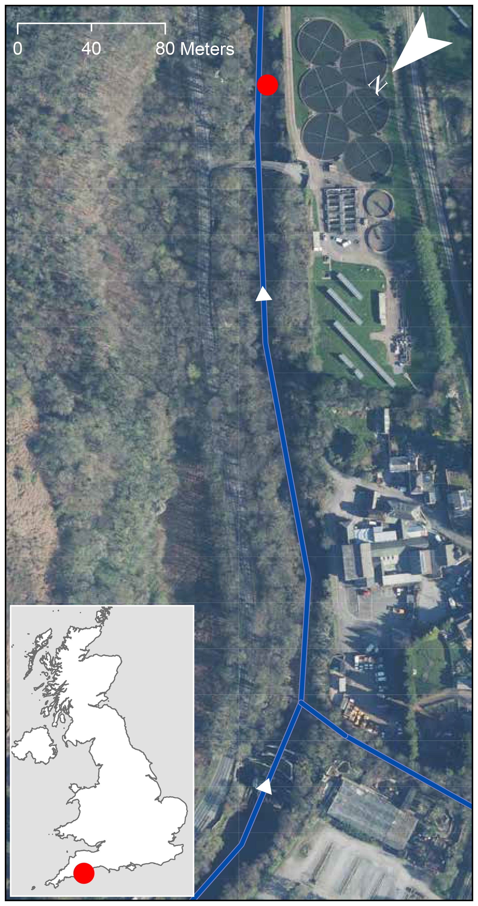
Figure 1 Location of the field experiment on the River Dart at Austins Bridge (red circle). River network and flow direction are shown by the blue lines and arrows, respectively. Aerial imagery provided by Getmapping: EDINA Aerial Digimap Service (2022). Inset map shows the monitoring location in the context of the UK.

2.2 Reference data

Whilst the flow gauging record at the experimental site began in 1959, the channel geometry and downstream control were modified by the 1979 flood. Therefore, for the purposes of this study we exclude reference flow measurements that were acquired prior to 1980. The reference data consist of river flow measurements (Q) that were made using a variety of approaches (Perks, 2025a). Of the 303 gauging measurements made between 1980–2018, 274 were obtained at the same stage as when a video was recorded (±0.01 m). Of these 274 measurements, 25 used an aDcp (stationary or moving-boat method), with the remainder using a combination of mechanical and digital impeller-type devices (e.g. OTT C31). Non-aDcp measurements were acquired using a single-point measurement at either 0.5D (22 %), 0.6D (78 %), or the surface (<1 %), with subsequent application of the velocity–area method. These data were collected by either wading in-stream (46 %) or deploying the measuring device from the permanent cableway present (54 %). Wading measurements were made in the stage range of 0.243–0.544 m, which is equivalent to a discharge range of 1.3–4.6 m³ s⁻¹. Beyond these low flows and up to the peak gauged stage of 2.27 m (equivalent to a flow rate of 145 m³ s⁻¹), the cableway was used for gauging. The lower end of the gauged range represents flow conditions that approximate the long-term 95 % exceedance value, whereas the highest flows analysed are of greater magnitude than the long-term 1 % exceedance value (UK CEH, 2024). For comparison with the 1-D flow estimates obtained with KLT-IV, we convert the reference Q value to a 1-D reference velocity [U_a] by dividing Q over the cross-sectional area, which is calculated from stage measurements at the time of gauging and geodetic cross-section surveys. The 1-D velocities (U_a) determined from the 274 Environment Agency gauging measurements range from 0.12 to 2.33 m s⁻¹, with a median of 0.39 m s⁻¹. River flows with lower velocities are more frequently gauged than are periods of higher velocity, resulting in the gauged data being positively skewed (skewness value of 1.2). Of the gauged flows, 24 % have U_a in excess of 1 m s⁻¹ and 5 % have U_a in excess of 2 m s⁻¹. This is indicative of the challenges associated with acquiring flow gauging data using standard operating procedures under high-flow conditions.

2.3 Image acquisition

The image acquisition hardware consists of an obliquely mounted HikVision DS-2CD2T42WD-I8 6 mm IP camera connected via Ethernet cable to a Raspberry Pi model 3B. The camera is located on the true right bank at a height of 4.75 and 2.55 m above the water surface at the minimum and maximum observed river stage, respectively. The camera is mounted at an oblique angle of 77° from nadir. Despite the adoption of an oblique camera angle, the camera does not observe between 4.6 and 8.6 m of the water surface (in the near distance). This accounts for between 21 %–26 % of the cross-section across the full range of flow conditions observed in this study (Fig. 2). The images are acquired at a resolution of 1920 × 1080 px at a rate of 19.99 ± 0.5 Hz (95 % confidence interval; Perks, 2024b). The image sequences are of 10 s duration and collected at 15 min intervals. In this analysis we utilise videos obtained during daylight hours between March 2018 and March 2019. Low-light and nighttime imagery (determined when infrared sensing was triggered) was removed due to inconsistent visibility of surface features. The first 3 s of each recording was eliminated from the analysis as the associated frames experienced compression and frame rate issues.

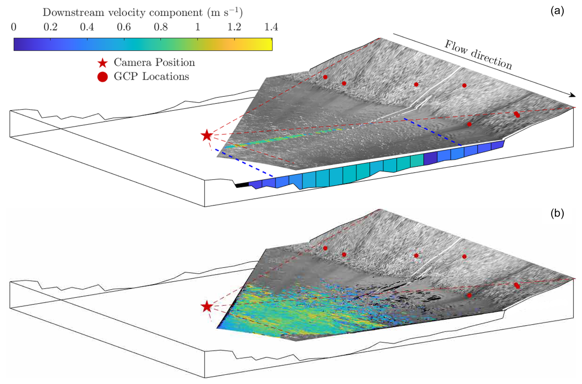
Figure 2 Schematic illustrating the monitoring station setup and the camera's partial view of the river cross-section. Cross-section data are presented up to the maximum observed river level. Dashed red lines illustrate the camera's field of view. The image presented is an orthophoto produced from footage acquired on 29 December 2018 at 13:00 GMT, when the flow discharge was ≈12 m³ s⁻¹ and section-averaged flow velocity was ≈0.54 m s⁻¹. Vectors represent the direction and velocity of (a) only those features that pass through the cross-section of interest and (b) all tracked features within the region of interest. Vectors coloured black are trajectories that have been filtered. In the application of theoretical flow field distributions (a; Sect. 2.6.1), surface velocity data are converted to a depth-averaged velocity before being binned into one of 20 equal-width cells, enabling the cell-averaged velocity to be obtained. Blue dashes represent the spatial extent of the detected surface features, and extrapolation of the flow field is required beyond this extent. The foundation of the velocity index approach (b; Sect. 2.6.2) is that the average surface velocity from across the field of view can be linearly related to the 1-D velocity.

2.4 Image calibration

Prior to image analysis, a site-specific camera model was developed to mathematically describe intrinsic parameters (e.g. focal length, lens distortion) and external parameters (e.g. location and orientation) (Messerli and Grinsted, 2015; Perks et al., 2016). This was required to enable transformation from image coordinates to geographic coordinates. Within KLT-IV the user must provide the following: (i) the surveyed location of ground control points (GCPs), (ii) initial estimates of the camera location $[x,y,z]$ and orientation, and (iii) the known height of the water surface being sensed. The user may also provide the intrinsic parameters of the camera if known. In order to calculate the intrinsic parameters of the camera model (i.e. radial and tangential distortion coefficients, camera focal length, and image centre parameters), geometric calibration was conducted using an 841 × 1189 mm checkerboard pattern and the Camera Calibrator App within MATLAB 2019b (The MathWorks Inc., 2022). A total of 40 images were used in this process, which resulted in a mean re-projection error of 0.61 px. The pixel coordinates of nine GCPs across the camera's field of view were obtained from imagery acquired by the HikVision camera, and the geographical coordinates of the GCPs were determined through acquisition of a high-spatial-resolution point cloud using a Leica MS50 multi-station. The dynamic nature of the water surface elevation over time is taken into account by automatically setting the water surface representation ($z_{m_{[x,y]}}$). This was achieved through the definition of the water surface elevation from the point cloud at the time of the survey (S_initial), the river stage at the time of survey (h_initial), and continuous river stage measurements performed using a float and counterweight shaft encoder at 15 min intervals (h):

$$\begin{array}{}\text{(1)}& z_{m_{[x,y]}}=S_{\mathrm{initial}}+(h-h_{\mathrm{initial}}).\end{array}$$

The camera location $[x,y,z]$ and view direction [yaw, pitch, roll] were initially estimated using the point-cloud survey. These characteristics were then defined as free parameters and optimised to minimise the square projection error of the GCPs using a modified Levenberg–Marquardt algorithm (Fletcher, 1971; Messerli and Grinsted, 2015).

2.5 Image processing

Prior to image velocimetry analysis, image sequences were orthorectified using the optimised camera model described in Sect. 2.4 and exported with a pixel size of 0.01 m × 0.01 m. Subsequently, these were subject to pre-processing to enhance the visibility of surface features. Specifically, high-frequency components of the orthorectified imagery were enhanced through application of a high-pass filter with a kernel size of 32 px × 32 px. This was achieved by calculating a low-passed version of the original image and subtracting it from the original (Thielicke and Sonntag, 2021). Additional inputs were also defined including the region of interest to ensure that areas of the image containing on screen display information (e.g. timestamp) and areas consisting of artificial noise (e.g. tree branches) were excluded from the analysis. The primary flow direction was also defined to enable both the primary and the secondary components to be computed.

The workflow for image velocimetry analysis consists of the automatic detection of naturally occurring surface water features using a minimum-eigenvalue algorithm (Shi and Tomasi, 1994). Features were subsequently tracked from frame to frame using a MATLAB implementation of the Kanade–Lucas–Tomasi algorithm (Lucas and Kanade, 1981; Tomasi and Kanade, 1991; Shi and Tomasi, 1994; Perks, 2020). The adopted approach tracks windows of features of 31 px × 31 px in size, from which an affine motion field is generated to assign velocities to different points within the window. Instances with pixel motion of lengths greater than the pre-defined window size are handled through the use of pyramid levels (Bouguet, 2000). This approach effectively down-samples the original image by a factor of 2 between each pyramid level; three pyramid levels were used in our analysis. The lowest pyramid level provides an initial estimate of the pixel displacement using the coarsest imagery. This is then refined in a recursive fashion through the pyramid levels up to the original image resolution (Bouguet, 2000).

Evaluation of feature tracking success is achieved through implementation of a forward–backward error propagation scheme. Firstly, forward trajectories are computed and stored based on apparent feature movement from the first to the last frame in the sequence. These trajectories are then compared with those derived by backward-tracking the feature from the last to the first frame in the sequence. If the difference between the trajectories exceeds 1 px, the trajectory is considered incorrect and removed from analysis (Kalal et al., 2010).

Features are tracked over a period of 0.50 s (10 frames), from which the start and finish positions (in metric units) are stored. These are converted to displacement rates (m s⁻¹) and broken down into their downstream and secondary velocity components. Two post-processing approaches are implemented to filter spurious vectors, namely the removal of (i) vectors that deviate from the user-defined flow line by ≥45° and (ii) vectors with a (user-defined) displacement of <0.1 m s⁻¹. The former acts to filter those vectors that are likely spurious based on their direction, whereas the latter filters objects that are close to being stationary. These typically represent objects located on the channel margins or reflections on the water surface (e.g. bank-side reflections observed in Fig. 2b).

2.6 Experimentation

Upon the reconstruction of the surface velocity field, it is common for these observations to be converted to data that describe the depth-averaged velocity at multiple points in the cross-section. This forms the basis for the widely adopted velocity–area method of flow discharge calculation (Herschy, 2014). However, when applying image velocimetry techniques in natural fluvial settings, it may not be possible for equidistant velocity measurements to be extracted from across the full channel width (e.g. Peña-Haro et al., 2021; Hutley et al., 2023). Gaps in measurements can be caused by variability in lighting, inhomogeneous tracer distribution, reduced pixel resolution of the far field, or the field of view failing to capture the active channel width (as evident in Fig. 2a). Several approaches have been adopted to account for these failings, which commonly involve either interpolation between cells of missing data or extrapolation beyond the observations through utilisation of theoretical flow field distributions (Leitão et al., 2018; Le Coz et al., 2010; Fulford and Sauer, 1986). Conversely, an alternative approach for converting the information contained within the surface velocity flow field to a flow velocity that is representative of the cross-section is through the development of empirical relationships between observed and reference observations (e.g. adoption of an index-velocity approach (Levesque and Oberg, 2012) or application of entropy theory (Chiu, 1989; Moramarco and Singh, 2010; Bahmanpouri et al., 2022; Vyas et al., 2024; Nord et al., 2025)). Here we test these two distinct approaches, which are described in the following sections and conceptualised in Fig. 3.

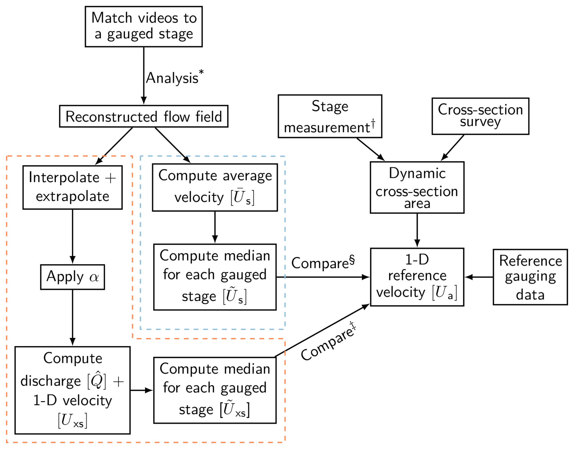
Figure 3 Schematic diagram illustrating the workflow of the data analysis as described in Sect. 2.6. ^* Analysis settings are described in Sect. 2.3–2.5. Items within the red box relate to the methods presented in Sect. 2.6.1, and items in the blue box are related to Sect. 2.6.2. ^† Derivation of river stage measurements in the local coordinate system are shown in Eq. (1). ^‡ Results are presented in Sect. 3.1. ^§ Results are presented in Sect. 3.2.

2.6.1 Utilisation of theoretical flow field distributions

In order to interpolate between and extrapolate beyond the extent of the surface velocity field, one of several assumptions about the flow field may be employed. Here we adopt three approaches: an assumption that the Froude number is constant within a cross-section (Le Coz et al., 2010; Fulford and Sauer, 1986) and the adoption of quadratic and cubic polynomials (Leitão et al., 2018). To apply the constant-Froude-number approach, linear regression between cell depth and cell average velocity was performed with the model intercept constrained to zero. For cells with missing data, velocities were estimated by multiplying the cell depth with the slope of the linear function. Where quadratic or cubic polynomials were used to estimate velocities in cells with missing data, data fitting was performed using the paired measurements of distance along the section- and cell-averaged velocity, with the addition of velocity values of zero at the channel boundaries. Cells in the section with missing values were subsequently estimated using the obtained quadratic or cubic polynomial function. Upon application of these techniques, average velocities for 20 cells of equal width were established (Fig. 2a). This was then converted to a depth-averaged velocity using a conversion factor (α) of 0.87. This site-specific value was obtained following analysis of 60 aDcp transects acquired between 2009 and 2018 (Perks, 2025d). Subsequently, the average cell velocity is multiplied by the cell area to give the unit discharge of each cell from which the flow discharge estimate at the cross-section of interest is obtained. This discharge value is divided by the wetted cross-sectional area to provide the image-based section-averaged (or 1-D) velocity (U_xs).

Our analysis focuses on the comparison between U_xs and the section-averaged (1-D) velocities derived from reference observations U_a. A total of 274 reference observations were made at the same stage as when videos were acquired (±0.01 m), spanning the flow discharge range of 1.27–145 m³ s⁻¹. To calculate the (1-D) velocities derived from reference flow gauging measurements, we simply divide the measured discharge by expected cross-sectional area based on a combination of the measured river stage and geodetic surveys. This approach is adopted even in the case where aDcp gauging measurements act as the reference flow data due to the potential for bias in cross-section measurements from aDcp data (discussed in Sect. 4.2). For each of the reference measurements, videos acquired at the same river stage (±0.01 m) are selected, and the medians of the 1-D velocities ${\stackrel{\mathrm{̃}}{U}}_{\mathrm{xs}}$ are used for further analysis. Additionally, a comparison between the KLT-IV depth-averaged velocities and SonTek RiverSurveyor M9 aDcp velocities is presented for eight flow gauging measurements. The choice of video to compare with the aDcp gauging data was based on the selection of U_xs that corresponds most closely with ${\stackrel{\mathrm{̃}}{U}}_{\mathrm{xs}}$ for the same flow stage as when the aDcp data were acquired (±0.01 m).

2.6.2 Index velocity

Using a combination of traditional flow gauging measurements and KLT-IV-derived velocities, relationships between the mean surface velocity from across the camera's field of view (index velocity, ${\stackrel{\mathrm{‾}}{U}}_s$) and the reference velocity (U_a) can be generated. This was initially calculated for the calibration period (March–June 2018) and then applied and tested for the validation period (July 2018–March 2019). During these time periods, videos were selected for analysis that were acquired at river levels coinciding with those of the available flow gauging measurements (±0.01 m). During the calibration period, 214 reference observations were made at the same stage as when videos were acquired, spanning the flow discharge range of 1.58–105 m³ s⁻¹. During the validation period, 274 reference observations were made at the same stage as when videos were acquired, spanning the flow discharge range of 1.27–145 m³ s⁻¹. For each video, ${\stackrel{\mathrm{‾}}{U}}_s$ was calculated and the median for each river level corresponding to a reference flow gauging measurement was computed [${\stackrel{\mathrm{̃}}{U}}_s$]. The derived ${\stackrel{\mathrm{̃}}{U}}_s$ values were compared with U_a through the application of least-squares regression between the two variables (Sect. 3.2).

Given the required calibration step, the sensitivity of the calibration to the number of U_a observations is evaluated. The number of measurements used in the calibration (n) ranged from 1–50. For each simulation a random 1-D reference velocity U_a was selected. Simultaneously, one ${\stackrel{\mathrm{‾}}{U}}_s$ value, obtained at the same river stage as when the reference gauging took place, was also sampled with replacement. For each pairing, the difference between ${\stackrel{\mathrm{‾}}{U}}_s$ and U_a is calculated, and the mean percent difference [D_k] is calculated as the number of flow gauging measurements is iteratively increased ($n=\mathrm{1}:\mathrm{50}$). These simulations were executed 100 000 times to account for the effects of sample size.

$$\begin{array}{}\text{(2)}& D_k={\displaystyle \frac{\mathrm{1}}{n}}\sum _{i=\mathrm{1}}^n({\stackrel{\mathrm{‾}}{U}}_{s_i}-U_{a_i})/U_{a_i}\cdot \mathrm{100}\end{array}$$

Values of the samples selected for each step of the calibration (n=1–50) are conditioned by the frequency distribution of the gauging data, with the likelihood of sampling a particular value being dependent on its frequency in the population. Inevitably, few flow gauging measurements are obtained at the highest flow magnitudes, with the median of the gauged discharge values being 6 m³ s⁻¹. Therefore, the calibration sample protocol reflects the distribution of the actual flow gauging record.

3 Results

3.1 Velocity reconstruction

When we consider the relationships between ${\stackrel{\mathrm{̃}}{U}}_{\mathrm{xs}}$ and U_a, we can identify strong linear relationships (r²=0.95–0.96), with the linear models having intercepts ranging from −0.01 to 0.032 and slopes ranging from 1.029 to 1.091 (Fig. 4). The model coefficients presented indicate that at U_a values >0.59 m s⁻¹, the constant-Froude-number approach produces velocity estimates in closest agreement with the reference velocity (Fig. 4c). At U_a values <0.59 m s⁻¹, the quadratic function performs objectively better than the constant-Froude-number approach but by no more than 0.03 m s⁻¹. The performance of the quadratic model (Fig. 4a) and cubic model (Fig. 4b) for interpolation and that of extrapolation of missing data within the cross-section are comparable. For each of the fitting methods adopted, ${\stackrel{\mathrm{̃}}{U}}_{\mathrm{xs}}$ generally underestimates relative to U_a. However, this relationship is not constant, with some variability observed. Taking the constant-Froude-number approach as an example, at reference velocities of between 0.12 and 0.5 m s⁻¹, 1-D estimates differ from the reference values by +12.5 %, by −20 % between 0.5 and 1.0 m s⁻¹, and by −10 % between 1.0 and 2.0 m s⁻¹, and they differ by −0.8 % for reference velocities in excess of 2.0 m s⁻¹.

Comparison of velocity profiles generated by SonTek RiverSurveyor M9 aDcp to those produced using KLT-IV provides further insight into the variation between modern hydrometric methods (, ) and the image-based approach. Overall, the mean absolute percentage error of the 1-D velocity estimates derived from the available SonTek M9 aDcp data and IV outputs is 9.8 %, with the aDcp and KLT-IV profiles being most similar under high-flow conditions (Q=48–101 m³ s⁻¹; Fig. 5a–b). For most examples, the area of the cross-section most proximal to the camera (distance of 10–20 m from left bank) generally closely corresponds to the aDcp data. However, there are exceptions to this. Under the highest-flow conditions (shown in Fig. 5a–b), the velocities in the near field of the imagery are not reconstructed accurately, with overestimations of up to 50 % (in the case of panel a) and underestimations of up to 75 % (in the case of panel b). In addition, whilst we observe that the constant-Froude-number extrapolation procedure works well in the majority of cases (Fig. 5a–e), there are significant overestimations in the far field of the imagery observed under low-flow conditions (Q=3–7 m³ s⁻¹; Fig. 5f–h). Potential sources of these errors are discussed in Sect. 4.3.

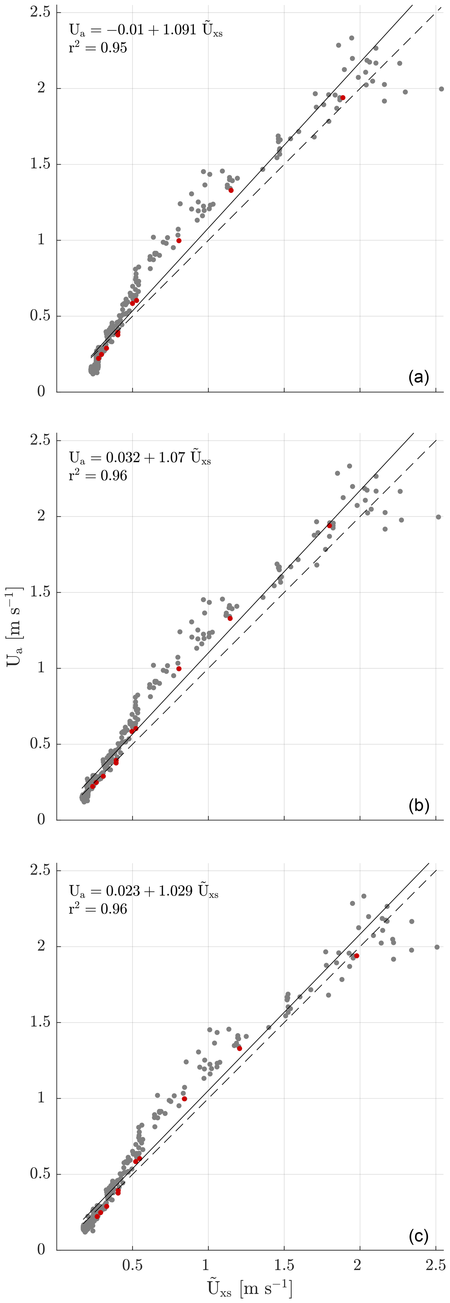
Figure 4 Relationship between the image-based 1-D flow velocity (${\stackrel{\mathrm{̃}}{U}}_{\mathrm{xs}}$) and 1-D flow velocity derived from Environment Agency flow gauging measurements (U_a). Interpolation between and extrapolation beyond observed cross-section velocities is achieved using (a) a quadratic function, (b) a cubic function, and (c) a constant-Froude-number assumption. Red dots are used to show the ${\stackrel{\mathrm{̃}}{U}}_a$ values that are plotted in Fig. 5.

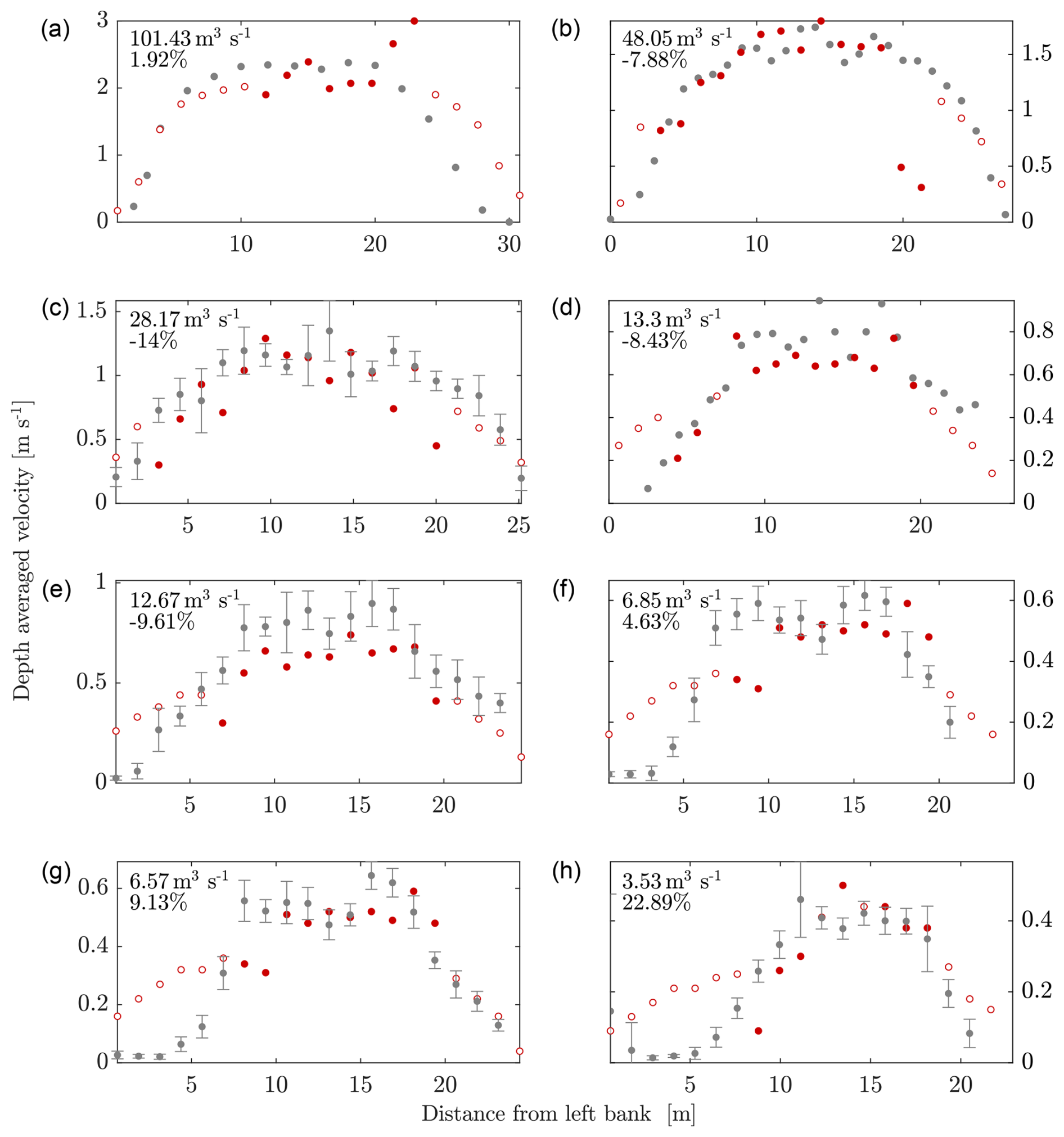
Figure 5 A selection of cross-section velocities illustrating the deviation between the SonTek aDcp velocity magnitudes (grey circles) and KLT-IV-generated velocities for a range of flow conditions. Measured velocities are shown by the filled red circles, whereas estimates based on the constant-Froude-number assumption are shown by the open red circles. Error bars illustrate the standard deviation of stationary aDcp measurements. Flow discharge measurements for the aDcp transects along with the percent difference between discharge reported by aDcp and the reconstructed discharge using KLT-IV are presented in each subplot.

3.2 Application of index velocity

The hydrological conditions observed during the calibration period led to the retention of 214 flow gauging measurements that were acquired at the same river stage (±0.01 m) as the videos. This serves as a calibration dataset to enable the partial view of the camera to be accounted for. As a consequence of (i) the camera's field of view failing to capture the entire cross-section and (ii) surface velocities being reconstructed as opposed to the depth-averaged velocities, it was initially hypothesised that ${\stackrel{\mathrm{‾}}{U}}_s\ne U_a$. To first explore the nature of this relationship, the deviation between ${\stackrel{\mathrm{‾}}{U}}_s$ and U_a is simulated. When only one U_a value is used to calibrate ${\stackrel{\mathrm{‾}}{U}}_s$, the data indicate that ${\stackrel{\mathrm{‾}}{U}}_s$ overestimates relative to U_a by 26 %; however, there is a great deal of variability in the outcome, with the IQR spanning 36 % (Fig. 6). As the number of U_a values used in the calibration increases, the variability is reduced, with the median percentage difference becoming stabilised when eight flow gauging measurements are used. In this scenario, the median output corresponds closely to that when 50 flow gauging measurements are used (27.4 % vs. 26.7 %). This analysis indicates that ${\stackrel{\mathrm{‾}}{U}}_s$ has a tendency to overestimate relative to U_a and that the relationship between these two variables is influenced by the number of flow gauging measurements that are used to predict the relationship.

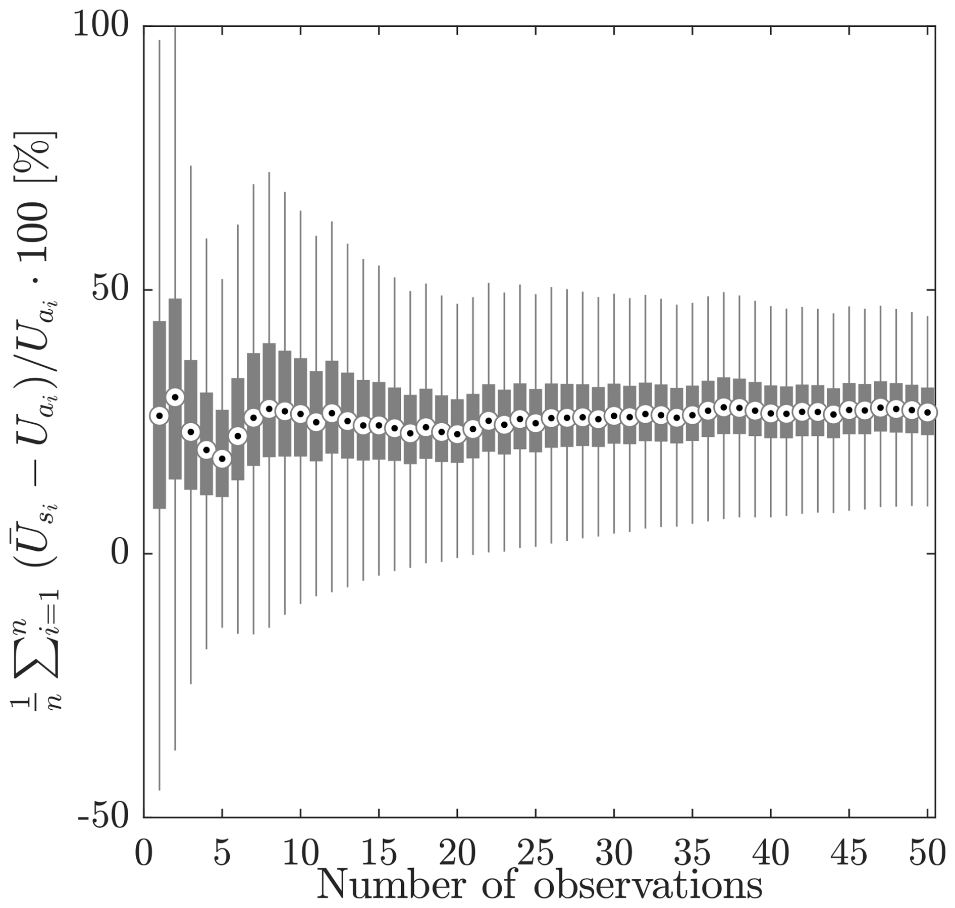
Figure 6 Results of Monte Carlo simulations, where the number of paired selections of U_a and ${\stackrel{\mathrm{‾}}{U}}_s$ are varied to determine their influence on the calibration of the KLT-IV approach.

This overestimation of ${\stackrel{\mathrm{‾}}{U}}_s$ relative to U_a is further highlighted when all 214 reference velocity measurements (U_a) are compared with the median of the distributed velocity measurements for the same river stage ${\stackrel{\mathrm{̃}}{U}}_s$. In this instance, a strong linear relationship (r²=0.96; p<0.001) can be observed (Fig. 7a). However, ${\stackrel{\mathrm{̃}}{U}}_s$ overestimates relative to U_a by 16 % on average. The calculation of the offset between ${\stackrel{\mathrm{̃}}{U}}_s$ and U_a is subsequently applied to the ${\stackrel{\mathrm{̃}}{U}}_s$ measurements obtained during the validation period (n=274), resulting in a much closer correspondence between the two variables (r²=0.98; p<0.001, Fig. 7b). This finding indicates that the applied transformation developed during the calibration period holds true beyond that period with an acceptable level of uncertainty.

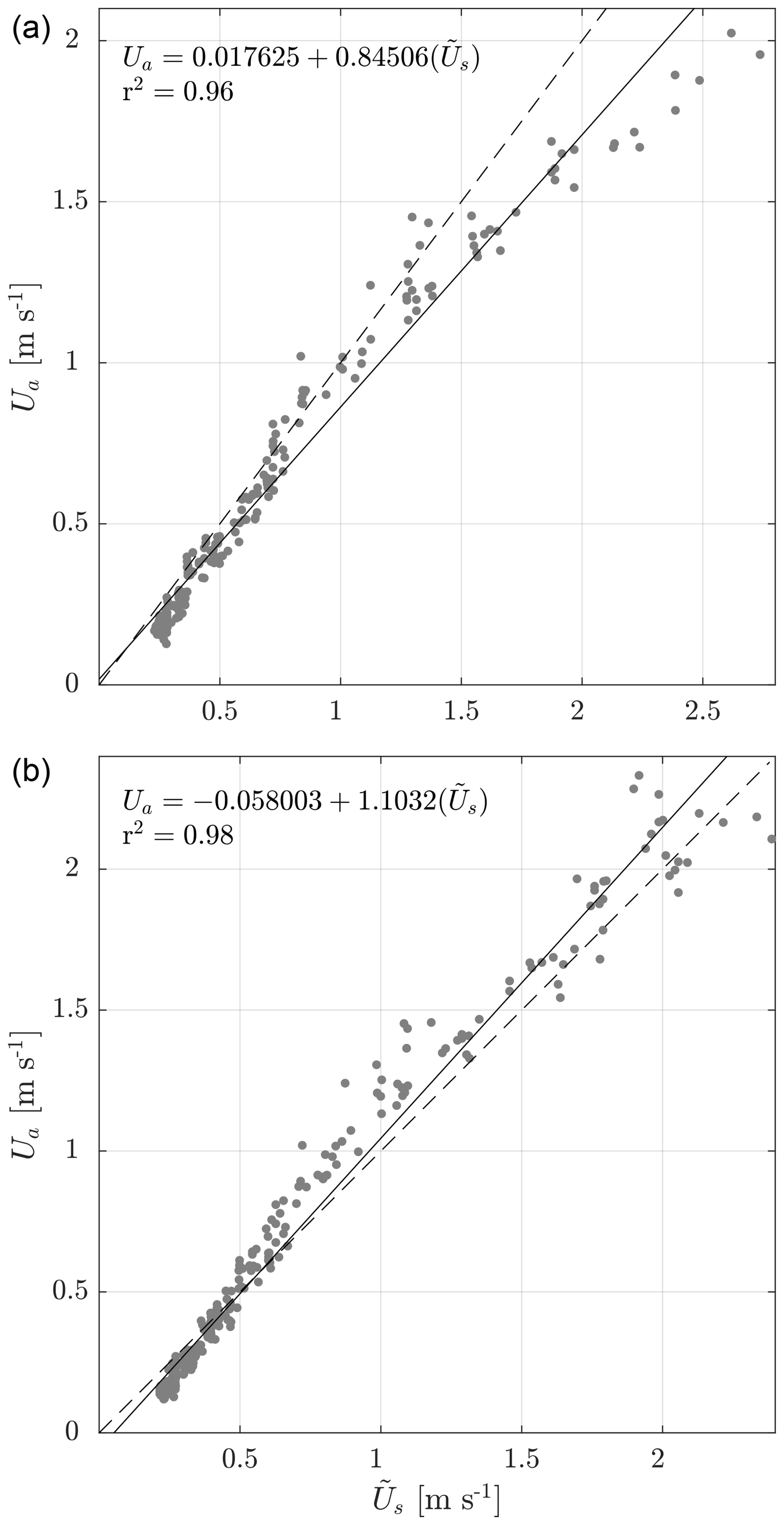
Figure 7 Bi-plot and linear fit between KLT-IV-derived velocity measurements [${\stackrel{\mathrm{̃}}{U}}_a$] and reference velocity measurements [U_a] during (a) the calibration period and (b) validation period. The solid line represents the linear fit between variables, with the 1:1 line also shown (dashed line).

4 Discussion

4.1 Application

Whilst this article has examined the inter-comparability of 1-D velocities obtained by image-based approaches and reference measurements made via a variety of methods (e.g. current flow meter, aDcp), the utility of 1-D measurements obtained by image velocimetry techniques is likely to be in the development or refinement of stage–discharge rating curves. When we utilise the velocity data obtained by either the constant-Froude-number assumption or the distributed index-velocity approach, we are able to generate discharge estimates that are broadly comparable with those generated by the standard Environment Agency flow gauging approaches (Fig. 8). When the relationship between image-based and reference gauging data is evaluated using a linear model with intercept of 0 and slope of 1, the coefficient of determination (r²) values for the constant-Froude-number assumption and the distributed index-velocity approach are 0.98 and 0.99, respectively, with root mean squared error (RMSE) values of 4.57 and 4.05 m³ s⁻¹, respectively, and a percent bias (PBIAS) of 5.5 % and 3.4 %, respectively (Fig. 8b). The particular utility of this approach is that image velocimetry analysis can be conducted in an autonomous environment following camera calibration, with inputs of a water level time series that correspond to the time of video acquisitions. However, additional information such as the cross-section geometry and an estimate of α to convert water surface to depth-averaged flow velocities or information relating the surface velocity from across the image with a section-averaged velocity is also required. When it is considered that the reference data used represent significant efforts of hydrometry teams to make field measurements in a range of challenging conditions between 1980–2018 and that the imagery used in this analysis was acquired for under 1 year and autonomously analysed in an unsupervised workflow, we can begin to identify the potential gains that wider employment of these techniques in appropriate environments may bring.

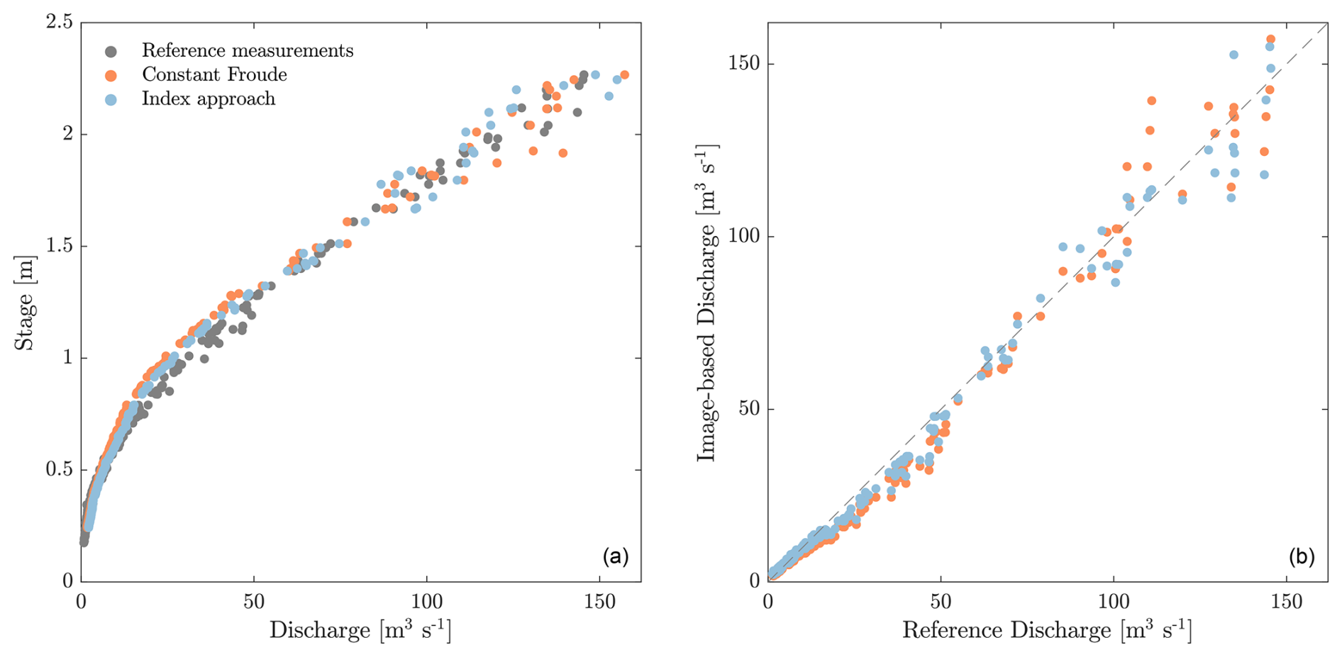
Figure 8 (a) Stage–discharge plots for the River Dart at Austins Bridge (UK) following analysis of imagery acquired over a 1-year period (shown in the red and blue) and developed using conventional flow gauging techniques between 1980–2018 (grey). (b) Comparison between image-based discharge estimates and reference discharge estimates with 1:1 line shown.

4.2 Uncertainties in reference datasets

The comparisons conducted here have involved the computation of 1-D velocities using the observed Q divided by the cross-sectional area at the time of observation based on geodetic survey measurements. Our analysis indicates that over an 8-year period (2010–2018), the cross-section across the full range of flows varied by 5 %. There is therefore a degree of uncertainty concerning the stability of the cross-section across the time period for which reference gauging measurements were obtained (1980–2018). Any variability will have a direct influence on the reference 1-D velocities calculated. In addition, the wetted cross-section area calculated through the combination of geodetic survey and stage measurements has previously been found to differ from aDcp-derived cross-sectional areas, with cross-section-averaged depths being underestimated by between 6 %–9.5 % (Kim et al., 2015). In the present study, the mean percentage error between these cross-section measurement methods is 7 % (12.5 % for RDI StreamPro, 5 % for SonTek RiverSurveyor M9) ±10 % (95 % CI), which should be acknowledged as a potential source of uncertainty. In addition, given that the reference velocities used in this analysis have been acquired from as early as 1980, there are inherent uncertainties in the acquisition methods adopted that cannot be quantified.

4.3 Uncertainties in image analysis

Analysis of the aDcp transects enabled the computation of an α value relating surface velocity measurements to a depth-averaged velocity. Analysis shows this value to be 0.87 ± 0.07 (95 % CI), a value within the expected range for unmodified channels consisting of a gravel bed (Turnipseed and Sauer, 2010). Given that this value is anticipated to vary as a function of water depth or relative roughness, it is of interest that no clear relationship between stage and α is observed. This complexity exemplifies the importance of acknowledging the role of α in uncertainty assessments (Hauet et al., 2018).

The videos analysed here are of 10 s duration, of which the first 3 s was discarded due to frame rate and compression issues. This is a relatively short period of time for analysis to be undertaken, with research illustrating the potential benefits of analysing longer-duration videos (Pumo et al., 2021), especially under poor seeding conditions (Dal Sasso et al., 2018). Furthermore, if longer-duration videos are available, it may be possible to limit analysis to the image sequences with optimal seeding characteristics, which can lead to potential gains in accuracy (Pizarro et al., 2020a, b).

Determination of the intrinsic parameters of the HikVision DS-2CD2T42WD-I8 6 mm IP camera used in this study was achieved in controlled laboratory conditions prior to deployment. Whilst determining these parameters can reduce the degrees of freedom during the camera model optimisation process, it should be noted that the coefficients describing the lens are not necessarily stable. An assessment performed by Elias et al. (2020) found that the intrinsic parameters of low-cost cameras were prone to vary as a function of temperature. When imagery was acquired from cold (i.e. immediately after switching on the device), projection of 2-D image coordinates to 3-D object space resulted in significant errors of up to 0.1 m at a distance of 10 m. However, the study also found that when imagery was acquired following a warm-up period, errors were greatly reduced (0.01–0.02 m at a distance of 10 m). Whilst the HikVision DS-2CD2T42WD-I8 6 mm IP camera used in this study may have similar traits to those investigated by Elias et al. (2020), the camera received power from a mains outlet continuously, therefore minimising temperature-related errors during the initialisation process.

Determination of the external orientation parameters (EOPs) of the camera at the site of the experiment was achieved by optimising a camera model based on the distribution of GCPs surveyed at the time of installation. Our study assumes that the location of these GCPs is stable (in image space) throughout the experiment with no camera movement either within a single video capture or between video captures. To assess the stability of the camera orientation between the start and the end of the monitoring period (March 2018–January 2019), the pixel locations of clearly visible points (corners of stage boards located on the far bank) were manually extracted. Pixel locations of these features were found to be consistent between the video captures (between 1–2 px). These pixel offsets approximate 1–3 cm in real-world distances, which is within the general uncertainty of the registration process. In instances where placement of permanent GCPs allow, updating the camera model for each video acquisition would enable a time series of platform poses to be generated (e.g. Perks et al., 2024) and movement of the platform to be accounted for (e.g. Eltner et al., 2021). However, identification of targets with changeable visual appearance over time would need to be addressed in an unsupervised workflow. In terms of the stability of image sequences within a single video, the impacts of small frame-to-frame movements as a consequence of environmental conditions (e.g. wind) may have an impact on the quality of velocimetry reconstruction, and we do not seek to quantify these effects here. Our method of analysing multiple videos for a given flow stage and adopting the median of the 1-D velocity estimates for comparison purposes seeks to minimise the effects of outliers that may be generated as a result of adverse external environmental conditions.

In the generation of orthophotos which are subsequently analysed to determine feature displacement, an assumption is made that the water surface is planar. Under normal flow conditions, this assumption is valid. However, under high-flow conditions, surface waves of considerable height (≫10 cm) develop, resulting in variable water surface elevations throughout the domain. Given the perspective of the camera, these surface undulations may result in biased flow velocity estimates due to part of the downstream component being registered as normal to the main flow line or alternatively part of the normal component being registered as contributing to the downstream flow rate.

Given the requirement for this analysis to be unsupervised and automated, image enhancement was limited to application of a high-pass filter only. Given the wide range of environmental and lighting conditions across the 1-year monitoring period, the visibility of the water surface and associated tracers differed throughout. The choice of this procedure was to maximise the visibility of potential tracers; however, this also comes at the risk of enhancing noise locally. In some instances, such as when the riverbed is visible under low-flow conditions, additional image enhancement procedures would be beneficial, e.g. background subtraction. The choice of pre-processing procedures is dependent on the challenges that one is trying to resolve. Therefore, implementation within an automated workflow is non-trivial, and the development of methods for generalisation is worthy of further research.

A final assumption of the image-based approach is the presence of a stable channel cross-section and downstream control at the experimental site. Whilst there is evidence for significant geomorphic change at this site (in 1979), one of the reasons for this location being selected was due to the stability of the cross-section over the intervening years. This is indirectly evidenced by the presence of a stable flow rating curve (UK CEH, 2024). Furthermore, as reported, our analysis of repeat surveys in 2010, 2018, and 2020 indicates that the cross-section changed by no more than 5 % across the full range of flows experienced. However, at monitoring locations where the cross-section is unstable, error assessments should be conducted.

4.4 Outlook

Recent research has illustrated the precision of optical flow methods for reconstructing flow dynamics and highlighted their relative insensitivity to parameterisation (Pearce et al., 2020). This has naturally led to application of these techniques becoming increasingly widespread for the purposes of obtaining dense surface flow fields, with their adoption into continuous monitoring workflows now becoming established (e.g. Hutley et al., 2023). However, a significant challenge in the application of these methods within unsupervised workflows is the presence of environmental noise, which leads to either a reduction in successfully tracked tracers or the presence of successfully tracked features that cannot readily be related to the depth-averaged flow. Generally this is presented as (i) noise that impacts the quality of the imagery and visibility of the water surface (e.g. inhomogeneous lighting of the water surface, bright spots on the camera lens, precipitation), (ii) the water surface texture lacking sufficient detail to enable dense flow fields to be established, and (iii) environmental factors that influence the quality of the measurements (e.g. tracking of features affected by the presence of standing waves or wind-induced effects). In the research presented here, we have not sought to address these issues directly. However, to improve robustness of the outputs, further analysis could be undertaken to identify and apply appropriate seeding density metrics to evaluate the quality of entire videos, eliminate poorly seeded image sequences from analysis, or focus analysis on specific cross-sections within the imagery to improve the quality of reconstructions. Alternatively, the influence of optical noise may be reduced through application of dynamic weighting across the image scene (e.g. Cao et al., 2022). Furthermore, utilisation of surrogate information (e.g. wind speed and direction) may be used to identify time periods where wind shear may have significant effects on the apparent surface velocities, allowing corrections to be established and applied where required. The potential for optical flow methods to be improved through application of deep learning models is also significant. Ansari et al. (2023) provided evidence for a range of convolutional neural network (CNN) optical flow models (collectively termed RivQNet) to improve flow reconstructions in challenging environmental conditions. Further refinement and training of these methods may offer significant performance benefits.

5 Conclusions

In this study, we investigate the potential for an open-source toolbox (KLT-IV) to reconstruct the surface flow field of the River Dart (UK) for the purposes of estimating section-averaged (1-D) velocity in an unsupervised and autonomous workflow. Given the partial view of the channel that is visible from the camera sensing system (73 % of the channel width under normal flow conditions), application of appropriate data-fitting methods or the establishment of index-based approaches was required to interpolate within and extrapolate beyond the field of view. Following image acquisition over a period of 1 year and following analysis of over 11 000 videos, we can draw the following conclusions:

1. Highly significant linear relationships (r²=0.95–0.97) are established between reference 1-D velocities and those computed using KLT-IV in conjunction with data-fitting techniques. The intercept of these models ranges from −0.01 to 0.032, and slopes range from 1.029 to 1.091 (Fig. 4).

2. The mean absolute percentage error in 1-D velocities (using the constant-Froude-number assumption) relative to those errors produced using a SonTek RiverSurveyor M9 aDcp is 9.8 % (Fig. 5).

3. An index-velocity approach is developed which relates the mean of the observed flow field to the reference 1-D velocity. The form of this relationship was established during a calibration period spanning March to June 2018, and this was subsequently applied and tested for a validation period (July 2018 to March 2019). In the validation period, a highly significant linear relationship (r²=0.98) was obtained between the mean values of the flow field and the reference 1-D velocities (Fig. 7).

4. We use the best-performing data-fitting approach and index-based approach to estimate flow discharge at the monitoring site. When these are compared with the reference data obtained by the Environment Agency, r² values of 0.98 to 0.99 are obtained (for a linear model), with a percentage bias of between 3.4 % and 5.5 % (Fig. 8).

5. We identify uncertainties in both the reference datasets and the image-based analysis that may be of significance. For example, in the case of the reference data, we identify a bias in aDcp-based cross-section measurements relative to those made using geodetic surveys of 7 %; and in the case of the image-based analysis, we identify an α of 0.87 ± 0.07 (95 % CI) following analysis of aDcp profiles. However, this does not vary in a systematic way, which may influence the resulting conversions from surface velocity to a depth-averaged velocity.

6. This approach is well suited to being used in operational and real-time settings. This is due to the relatively few parameters that must be defined following initial set-up. In the present analysis all parameters are kept constant and not varied as a function of river stage. However, a thorough assessment of the dependency of flow field reconstructions with varying environmental and hydro-geomorphic conditions remains a research gap.