A distributed hybrid physics–AI framework for learning corrections of internal hydrological fluxes and enhancing high-resolution regionalized flood modeling

To advance the discovery of scale-relevant hydrological laws while better exploiting massive multisource data, merging artificial intelligence with process-based modeling has emerged as a compelling approach, as demonstrated in recent lumped hydrological modeling studies. This research proposes a general spatially distributed hybrid modeling framework that seamlessly combines differentiable process-based models with neural networks. Specifically, we focus on hybridizing the hydrological module – built atop a differentiable kinematic wave routing over a flow direction grid – using a process-parameterization network that refines internal water fluxes, with all conceptual parameters estimated by a regionalization network trained simultaneously. We evaluate flood modeling performance and analyze the interpretability of learned conceptual parameters and corrections of internal fluxes using two high-resolution datasets (dx=1 km and dt=1 h). The first dataset involves 235 catchments in France, used for local calibration–validation and model structure comparisons between the classical Génie Rural (GR)-like model and the hybrid approach. The second dataset presents a challenging multi-catchment modeling setup in flash-flood-prone areas to demonstrate the framework's regionalization learning capabilities. The results show that the hybrid models achieve superior accuracy and robustness compared to classical approaches in both spatial and temporal validation. Analysis of the spatially distributed parameters and internal fluxes reveals the hybrid models' nuanced behavior, their adaptability to diverse hydrological responses, and their potential to uncover physical processes.

1 Introduction

Faced with the socioeconomic challenges of flood and drought forecasting in the context of climate change, modeling approaches that make the most of the maximum amount of information available are needed to make accurate forecasts at high spatiotemporal resolution. Nevertheless, given the complexity and nonlinearity of the coupled surface and subsurface physical processes involved and their limited observability with respect to the number of parameters to estimate (“curse of dimensionality”), hydrological modeling remains a difficult task tinged with uncertainties (e.g., Liu and Gupta, 2007). Moreover, in the absence of directly exploitable first principles in hydrology (e.g., Dooge, 1986), as opposed to flow mechanistic equations in continuous media such as river hydraulics, meteorology, or oceanography, and given the high heterogeneities of continental hydrosystem compartments as well as the lack of “scale-relevant theories” (Beven, 1987), process-based hydrological models generally include a certain amount of empiricism, which represents an avenue for the fusion of data assimilation (DA) and uncertainty quantification (UQ) with machine learning (ML) and deep-learning (DL) techniques to better exploit the informative richness of multisource data.

Pure ML applications in hydrology started decades ago (e.g., references in Maier and Dandy, 2000, or Artigue et al., 2012, on flash floods). A recent explosion of artificial intelligence (AI) applications, stemming from the rise in big data, computational power, and capabilities to extract multilevel information from large datasets (LeCun et al., 2015), has led to a bloom of studies, in particular in hydrology, e.g., the reviews by Nearing et al. (2021) and Shen and Lawson (2021) and water-related disciplines (e.g., Tripathy and Mishra, 2024). The potential of using a long short-term memory (LSTM) network (Hochreiter and Schmidhuber, 1997), a recurrent neural network (RNN) adapted to long time series, for lumped continuous rainfall–runoff modeling was introduced by Kratzert et al. (2018) and explored in hundreds of studies since (Shen and Lawson, 2021). In addition to the capability of LSTM to learn multi-frequency aspects, training these networks over large catchment samples using meteorological forcing time series and catchment physical descriptors within lumped models enhances performance in daily runoff prediction and regionalization (Kratzert et al., 2018; Hashemi et al., 2022). A convolutional LSTM architecture, combining the strength of LSTM to capture multiscale temporal dynamics and convolutional layers for spatial pattern extraction, is found to be effective for spatiotemporal rainfall nowcasting (Shi et al., 2015) and hydrological modeling (e.g., Xu et al., 2022; Chen et al., 2022). Nevertheless, pure ML or DL algorithms are hardly interpretable and do not use effective physical models, solvers, and DA techniques developed over the past century. Hybrid approaches that leverage ML or DL in sequential combination with process-based numerical models via their inputs or outputs were explored recently and enable improvement in the accuracy of hydrological predictions (e.g., Konapala et al., 2020, with DA in Roy et al., 2023, or UQ in Tran et al., 2023).

Merging process-based differential equations with ML can be very advantageous, as recently shown with physics-informed neural networks (PINNs) in Raissi et al. (2019), where the process-based model is used as a weak constraint in the training cost function and is well adapted to assimilating observations (e.g., He et al., 2020) or universal differential equations that embed a universal approximator (Chen et al., 2019; Rackauckas et al., 2021; Yin et al., 2021). In hydrology, integrating ML into process-based models shows promise, as demonstrated in recent studies on daily lumped models (Kumanlioglu and Fistikoglu, 2019; Jiang et al., 2020; Höge et al., 2022; Feng et al., 2022). Kumanlioglu and Fistikoglu (2019) replaced the routing component of a lumped Génie Rural (GR) model (Perrin et al., 2003) – an algebraic model derived from temporally integrable ordinary differential equations (ODEs) – with an artificial neural network (ANN), achieving superior performance compared to using the GR model or ANN alone in a single basin. Including an ANN for flux correction in a spatially lumped process-based hydrological ODE (Höge et al., 2022) and adding an ANN-based regionalization pipeline (Feng et al., 2022) or a semi-lumped model (Li et al., 2024) has resulted in learnable lumped model structures that exhibit interesting performance and improved interpretability after training. However, these approaches do not inherently account for spatially distributed information, such as detailed meteorological forcings and descriptors of basin physical properties, which is crucially needed for high-resolution hydrological modeling, particularly for extreme events with strong variability.

A spatially distributed hybrid approach, HDA-PR (hybrid data assimilation and parameter regionalization), which incorporates a regionalization neural network into the forward model, was recently proposed by Huynh et al. (2024b). This approach has enhanced regional flash flood modeling at a relatively high resolution (dx=1 km and dt=1 h). Meanwhile, Wang et al. (2024) introduced a large-scale spatialized hybrid hydrological model that improves evapotranspiration modeling for the Amazon basin by incorporating a replacement neural network and a regionalization neural network. In their study, Wang et al. (2024) combined a conceptual hydrological model with a simple bucket-based routing structure, using a hybrid approach that predicts conceptual parameters and corrects evapotranspiration (adjusting a Penman–Monteith estimate via a 3D convolutional neural network – CNN) without correcting other internal fluxes, and it operates at a coarser resolution (dx=0.5° and dt=1 d). In addition, enhancing the physical modeling of runoff and flood propagation necessitates the use of hydraulic models that must be differentiable in order to facilitate gradient-based optimization, a requirement for effective hybrid modeling. This approach has been demonstrated for the optimization of large parameter sets from heterogeneous data at the river network scale using various approaches based on differentiable hydraulic models, including a 2D or multidimensional complete shallow-water model coupled to a differentiable semi-lumped GR model (Pujol et al., 2022), a 1D Saint-Venant river network model (e.g., Larnier et al., 2025, though without a differentiable hydrological model), and a kinematic wave model integrated into a grid differentiable spatialized hydrological model (Huynh et al., 2024a). These hydraulic models consist of partial differential equations (PDEs). Therefore, hybrid hydrological models embedding neural networks should advance from lumped, semi-lumped, or spatialized ODE-based models to spatially distributed differentiable hybrid PDE-based hydrological–hydraulic models with a view to improving modeling capabilities at the basin scale and their realism, at least for hydraulic processes whose modeling is less uncertain than hydrological processes occurring in Earth's critical zone (the near-surface environment where complex interactions between water, soils, rocks, and living organisms regulate Earth's surface dynamics).

To address the aforementioned challenges, this research proposes a spatially distributed hybrid modeling framework combining process-based models and neural networks that is amenable to hydrological–hydraulic (H&H) modeling and other geophysical models. This study is based on a spatially distributed, parsimonious GR-like hydrological model structure that is well suited to flood modeling and regionalization learning (Huynh et al., 2024b), coupled with a differentiable kinematic wave model for spatially distributed flow routing. The original version of this framework was first proposed in Huynh et al. (2024a), while the present article enhances the approach with a more comprehensive case study, testing a larger sample set and offering more detailed analyses. The research continues to focus on correcting internal fluxes via a simple neural network. A relatively parsimonious hybridization with a dense flux correction neural network is proposed, as it effectively captures nonlinear flux corrections while leveraging the memory effect already embedded in the original hydrological model. This reduces the need for recurrent architectures such as LSTM, which are typically designed for sequential data but introduce additional complexity that is unnecessary for this application. The approach is implemented in the SMASH (Spatially distributed Modeling and ASsimilation for Hydrology) platform (Colleoni et al., 2025) that enables multiscale modeling, numerical adjoint model derivation via automatic differentiation, and variational data assimilation (VDA). The performance, robustness, and interpretability of the proposed approach are studied at a relatively high spatiotemporal resolution of 1 km and 1 h, over a large sample of French catchments and also over a challenging flash-flood-prone area. This study aims to demonstrate the feasibility and advantages of distributed hybrid modeling for spatiotemporal learning of hydrological processes at basin and regional scales. It provides a general framework for PDE-based spatially distributed modeling, taking advantage of AI and big data.

2 Method

2.1 Forward differentiable spatially distributed model statement

The forward differentiable hybrid model ℳ is obtained by partially composing (i) a dynamic-process-based, differentiable, and spatially distributed rainfall–runoff model with simplified hydraulic routing ℳ_rr-hy with (ii) a learnable (neural-network-based), differentiable process-parameterization and regionalization operator ϕ, resulting in Eq. (1).

$$\begin{array}{}\text{(1)}& {\displaystyle }{\displaystyle }\mathcal{M}={\mathcal{M}}_{\text{rr-hy}}\left(.;\mathit{\varphi }\left(.\right)\right)\end{array}$$

Let Ω⊂ℝ² denote a 2D spatial domain with x∈Ω the spatial coordinate, $t\in \left]\mathrm{0},T\right]$ the physical time, and 𝒟_Ω an eight-direction (D8) drainage plan. The spatially distributed rainfall–runoff model ℳ_rr-hy is a dynamic operator projecting the input fields of atmospheric forcings 𝓘 onto the fields of surface discharge Q, internal states h, and internal fluxes q, as expressed in Eq. (2):

$$\begin{array}{ll}{\displaystyle }\mathit{U}(x,t)& {\displaystyle }=\left[Q,\mathit{h},\mathit{q}\right]\left(x,t\right)\\ \text{(2)}& {\displaystyle }& {\displaystyle }={\mathcal{M}}_{\text{rr-hy}}\left({\mathcal{D}}_{\mathrm{\Omega }},\mathcal{I}(x,t);{\mathit{f}}_q(x,t),\left[\mathit{\theta },{\mathit{h}}_{\mathrm{0}}\right]\left(x\right)\right),\end{array}$$

with U(x,t) the modeled state flux variables, f_q the vector of spatially distributed corrections of the internal fluxes q (which will be explained later), and θ and h₀ the spatially distributed parameters and initial states of the hydrological model. Note that neural-network-based estimation of initial states is also feasible, e.g., for short-range DA; however, this is beyond the scope of the current work.

A neural-network-based estimator ϕ, with trainable parameters ρ, is embedded in the hydrological model ℳ_rr-hy and forms part of the complete model ℳ. Its purpose is to predict corrections of internal fluxes f_q and to estimate parameters θ regionally based on various input data, including atmospheric forcings 𝓘 and spatialized physical descriptors 𝓓, as described in Eq. (3).

$$\begin{array}{}\text{(3)}& {\displaystyle }{\displaystyle }\mathit{\varphi }:(\mathcal{I},\mathit{h},\mathcal{D};\mathit{\rho })\to ({\mathit{f}}_q,\mathit{\theta },{\mathit{h}}_{\mathrm{0}})\end{array}$$

By design, the complete forward model ℳ is learnable through the neural-network-based mapping ϕ embedded in ℳ_rr-hy. Moreover, if ℳ_rr-hy and ϕ are differentiable, then ℳ is differentiable, which is required to obtain its output gradient derivatives with respect to the neural network parameters as needed for their optimization.

The differentiable spatially distributed hydrological model studied hereafter is based on ODEs for local runoff production coupled with neural networks. This runoff is then conveyed on the spatial grid with a PDE-based hydraulic model.

2.2 Case of a differentiable spatially distributed GR-like and kinematic wave model

The spatially distributed differentiable, learnable, and regionalizable model proposed and studied in this article is detailed in this section. Its hydrological component is based on GR4, which is a parsimonious, widely used, and efficient lumped hydrological model (Perrin et al., 2003). Interception, production, and fast and slow transfer branch structures are used at the pixel scale without unit hydrographs, which are not needed for small-scale pixels (Huynh et al., 2024b, and references therein) and could, if needed for a semi-distributed model with larger subcatchments, be replaced by a Nash cascade that is differentiable and quasi-equivalent (cf. Santos et al., 2018). Moreover, the selected hydrological operators simply consist of algebraic relations obtained from analytical integration in time of first-order ODEs that describe state evolution in interception, production, and transfer reservoirs plus closure laws. This simple hydrological model produces “runoff” at the pixel scale that is then routed on the spatial grid with a kinematic wave model (Te Chow et al., 1988). These model operators and their numerical implementation are fully differentiable, a property further detailed in the following sections. Additionally, this dynamical hydrological model, implemented as recurrence relations, maintains a spatiotemporal memory via the reservoir states h(x,t). This property is used to define the hybridization for internal flux corrections via a simple ANN based on the principle of parsimony. The ANN uses previous reservoir states and atmospheric forcings as inputs, which requires no additional information beyond the original model. The proposed model, which is spatially distributed and differentiable, is schematized in Fig. 1. The following sections describe the complete forward model, including details on the neural networks used for flux corrections and parameter regionalization.

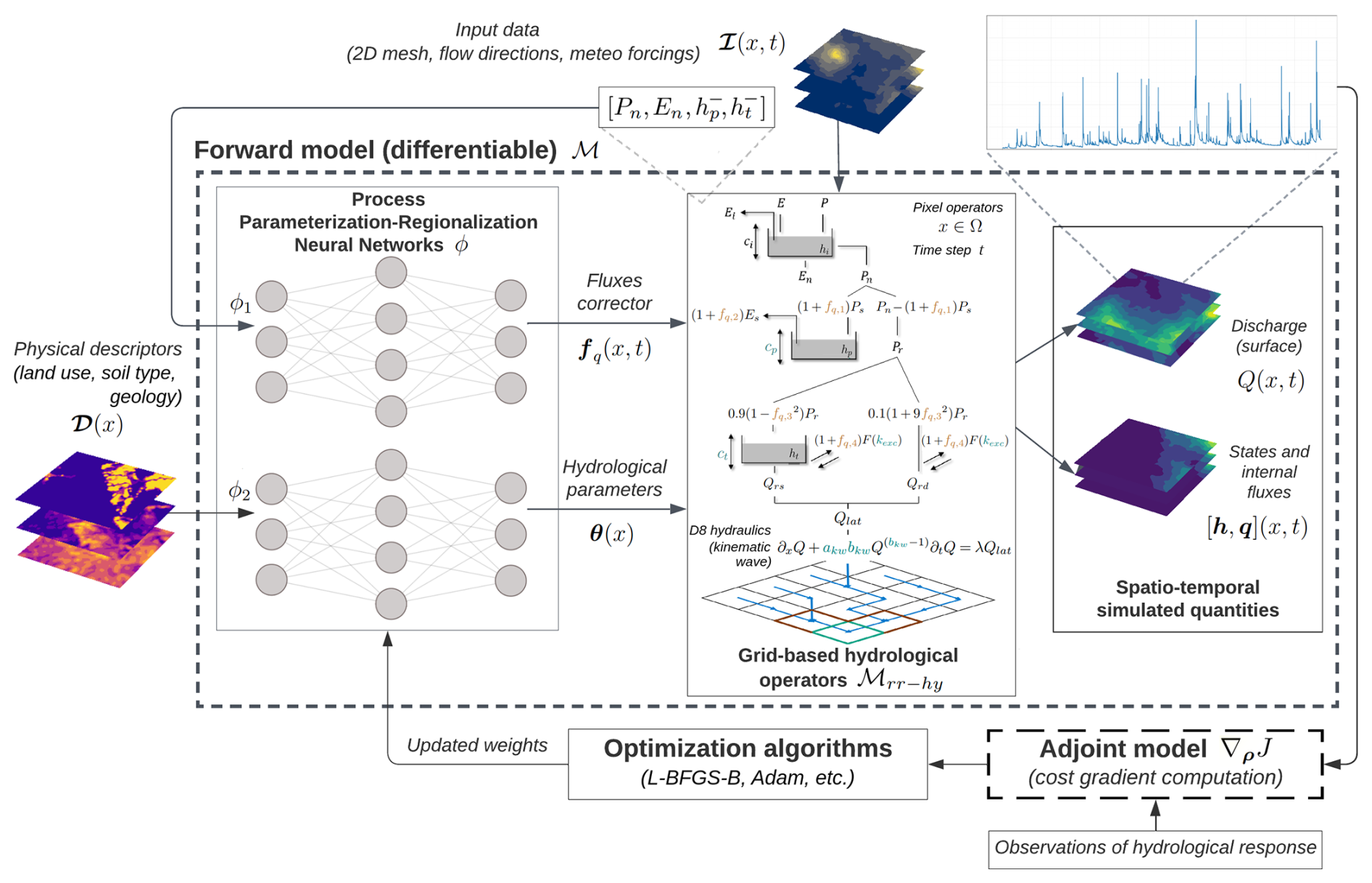
Figure 1 Hybrid physics–AI framework, applied to the spatially distributed GR-like and kinematic wave model, involving a pair of process parameterization and regionalization neural networks. The pair of neural networks is used to (i) correct internal fluxes with “neutralized” (by interception reservoir terminology of GR models from Perrin et al., 2003, and Santos et al., 2018) atmospheric data and (ii) estimate the model parameters using physical descriptors, with their weights optimized through high-dimensional optimization algorithms using an adjoint model to obtain accurate gradients of the cost function.

2.2.1 Runoff production

For a given cell x∈Ω and time step t>0, P(x,t) and E(x,t) represent the local precipitation and potential evapotranspiration. For simplicity, spatiotemporal dependencies on x and t are omitted in the following equations.

Interception. First, an interception reservoir of capacity c_i, automatically computed with the flux matching technique (cf. Ficchì et al., 2019), enables computation of the neutralized rainfall P_n and the neutralized evapotranspiration E_n.

Production. Then, the infiltration flux ${\stackrel{\mathrm{̃}}{P}}_s$ into the production reservoir is obtained by applying a correction term f_q,1, predicted by the neural network ϕ₁, to the classical GR infiltration flux P_s as follows:

$$\begin{array}{ll}{\displaystyle }& {\displaystyle }{\stackrel{\mathrm{̃}}{P}}_s=min(P_{\mathrm{n}},(\mathrm{1}+f_{q,\mathrm{1}}\left)P_s\right)\\ \text{(4)}& {\displaystyle }& {\displaystyle }\text{ with }{P}_s=c_{\mathrm{p}}\left(\mathrm{1}-{\left({\displaystyle \frac{h_{\mathrm{p}}^{-}}{c_{\mathrm{p}}}}\right)}^{\mathrm{2}}\right){\displaystyle \frac{\text{TanH}\left(\frac{P_{\mathrm{n}}}{c_{\mathrm{p}}}\right)}{\mathrm{1}+\left(\frac{h_{\mathrm{p}}^{-}}{c_{\mathrm{p}}}\right)\text{TanH}\left(\frac{P_{\mathrm{n}}}{c_{\mathrm{p}}}\right)}},\end{array}$$

where c_p represents the capacity of the production reservoir predicted by the neural network ϕ₂, and $h_{\mathrm{p}}^{-}$ is the production state at the previous time step. The actual evapotranspiration flux ${\stackrel{\mathrm{̃}}{E}}_s$ subtracted to the production reservoir is obtained by applying a correction term f_q,2, predicted by ϕ₁, to the classical GR evapotranspiration flux E_s as follows:

$$\begin{array}{ll}{\displaystyle }& {\displaystyle }{\stackrel{\mathrm{̃}}{E}}_s=min(E_{\mathrm{n}},(\mathrm{1}+f_{q,\mathrm{2}}\left)E_s\right)\\ \text{(5)}& {\displaystyle }& {\displaystyle }\text{ with }{E}_s=h_{\mathrm{p}}^{-}\left(\mathrm{2}-{\displaystyle \frac{h_{\mathrm{p}}^{-}}{c_{\mathrm{p}}}}\right){\displaystyle \frac{\text{TanH}\left(\frac{E_{\mathrm{n}}}{c_{\mathrm{p}}}\right)}{\mathrm{1}+\left(\mathrm{1}-\frac{h_{\mathrm{p}}^{-}}{c_{\mathrm{p}}}\right)\text{TanH}\left(\frac{E_{\mathrm{n}}}{c_{\mathrm{p}}}\right)}}.\end{array}$$

Transfer (subgrid). A subgrid transfer with slow and fast “lateral” flow components is fed by a learnable partition of net rainfall using a correction term f_q,3 predicted by ϕ₁, where the net rainfall $P_{\mathrm{r}}=P_{\mathrm{n}}-{\stackrel{\mathrm{̃}}{P}}_s$ is split into ${\stackrel{\mathrm{̃}}{Q}}_{\text{dl}}$ and ${\stackrel{\mathrm{̃}}{Q}}_{\text{dr}}$, representing the fluxes that feed the delayed and direct transfer branches:

$$\begin{array}{}\text{(6)}& {\displaystyle }{\displaystyle }{\stackrel{\mathrm{̃}}{Q}}_{\text{dl}}=\mathrm{0.9}(\mathrm{1}-f_{q,\mathrm{3}}^{\mathrm{2}})P_{\mathrm{r}}\text{ and }{\stackrel{\mathrm{̃}}{Q}}_{\text{dr}}=\mathrm{0.1}(\mathrm{1}+\mathrm{9}{f}_{q,\mathrm{3}}^{\mathrm{2}})P_{\mathrm{r}}.\end{array}$$

A nonconservative exchange flux $\stackrel{\mathrm{̃}}{F}$, applied to both the transfer reservoir and the fast transfer branch (direct runoff), is obtained by applying a correction term f_q,4, predicted by ϕ₁, to the classical GR exchange flux F:

$$\begin{array}{}\text{(7)}& {\displaystyle }{\displaystyle }\stackrel{\mathrm{̃}}{F}=(\mathrm{1}+f_{q,\mathrm{4}})F,\text{ with }F=k_{\text{exc}}\times {\left({\displaystyle \frac{h_{\mathrm{t}}^{-}}{c_{\mathrm{t}}}}\right)}^{\mathrm{7}/\mathrm{2}},\end{array}$$

where k_exc and c_t represent the exchange coefficient and the capacity of the transfer reservoir predicted by ϕ₂, and $h_{\mathrm{t}}^{-}$ is the transfer reservoir state at the previous time step. The outflow subtracted to the transfer reservoir is

$$\begin{array}{}\text{(8)}& {\displaystyle }{\displaystyle }{Q}_{\text{rs}}\left(t\right)=h_{\mathrm{t}}^{-}-{\left((h_{\mathrm{t}}^{-}{)}^{-\mathrm{4}}+c_{\mathrm{t}}^{-\mathrm{4}}\right)}^{-\mathrm{1}/\mathrm{4}}.\end{array}$$

The remaining net rainfall flux ${\stackrel{\mathrm{̃}}{Q}}_{\text{dr}}$ feeds the direct transfer branch where the exchange flux $\stackrel{\mathrm{̃}}{F}$ is also applied, and its outflow is $Q_{\text{rd}}={\stackrel{\mathrm{̃}}{Q}}_{\text{dr}}+\stackrel{\mathrm{̃}}{F}$. The hydrological runoff flux produced at the pixel scale is $Q_{\text{lat}}=Q_{\text{rs}}+Q_{\text{rd}}$ and is routed over a 2D mesh with a simple hydraulic routing module.

Note that the values of $f_{q,i=\mathrm{1}\mathrm{\dots }\mathrm{4}}$, which are the outputs of ϕ₁, are bounded between −1 and 1 (Sect. 2.2.3). Thus, by definition, the transformation functions applied to these internal flux corrections (i.e., $\mathrm{1}+f_{q,\mathrm{1}}$, $\mathrm{1}-f_{q,\mathrm{3}}^{\mathrm{2}}$, etc.) enable the preservation of the original conceptual model structure when the neural network output is 0, as all transformations equal 1 in this case. These terms were defined based on the specific fluxes being corrected and the mathematical constraints. For example, the correction f_q,3 is squared to ensure nonnegativity, and its transformations ($\mathrm{1}-f_{q,\mathrm{3}}^{\mathrm{2}}$ and $\mathrm{1}+\mathrm{9}{f}_{q,\mathrm{3}}^{\mathrm{2}}$) are specifically designed to preserve mass conservation in the transfer branch partitioning, as $\mathrm{0.9}(\mathrm{1}-f_{q,\mathrm{3}}^{\mathrm{2}})+\mathrm{0.1}(\mathrm{1}+\mathrm{9}{f}_{q,\mathrm{3}}^{\mathrm{2}})=\mathrm{1}$ for any value of f_q,3, while allowing the model to learn and adjust the partition between delayed and direct transfer branches from their default values of 0.9 and 0.1, respectively.

2.2.2 Pixel-to-pixel flow routing of runoff with a partial differential equation

The routing module used here is based on a conceptual 1D kinematic wave model that is numerically solved with a linearized implicit numerical scheme (Te Chow et al., 1988). The discharge routing problem is classically reduced to a 1D problem by considering a D8 drainage plan 𝒟_Ω(x), obtained by terrain digital elevation model processing with the condition that a unique pixel has the highest drained area.

The kinematic wave model is a PDE obtained by simplifying the 1D Saint-Venant equations assuming that the momentum reduces to a flow friction slope equal to the bottom slope. Using a conceptual parameterization of the momentum $A=a_{\text{kw}}{Q}^{b_{\text{kw}}}$ with A the flow cross-sectional area, Q the discharge, and a_kw and b_kw two parameters to be estimated and injecting this into the mass equation ${\partial }_{x}Q+{\partial }_{t}A=\mathit{\lambda }{Q}_{\text{lat}}$ with Q_lat the lateral discharge (total runoff produced at a pixel from GR operators) and λ the conversion factor, a single-equation model is obtained. The model is discretized with a classical finite-difference approach (cf. Te Chow et al., 1988), resulting in the following expression for the discharge propagation model:

$$\begin{array}{}\text{(9)}& {\displaystyle }{\displaystyle }{\partial }_{x}Q+a_{\text{kw}}{b}_{\text{kw}}{Q}^{(b_{\text{kw}}-\mathrm{1})}{\partial }_{t}Q=\mathit{\lambda }{Q}_{\text{lat}}.\end{array}$$

2.2.3 Learnable mappings for a spatialized GR-like model on top of kinematic wave routing

In this study, we use two multilayer perceptrons, the first ϕ₁ for spatiotemporal corrections of the model-internal fluxes f_q(x,t) and the second ϕ₂ for spatialized parameter θ(x) regionalization as used in Huynh et al. (2024b). That is, ϕ consists of a pair of neural networks designed to ingest (i) neutralized atmospheric inputs ${\mathcal{I}}_{\mathrm{n}}=(P_{\mathrm{n}},E_{\mathrm{n}})$ (using the wording of the GR conceptual model in Perrin et al., 2003; Santos et al., 2018), along with the model states at the previous time step $\mathit{h}(x,t-\mathrm{1})$, to correct the spatiotemporal internal fluxes q (process-parameterization pipeline) and (ii) physical descriptors 𝓓 (refer to Appendix A for information on the studied descriptors) to estimate the spatialized hydrological parameters θ (regionalization pipeline), as shown in Eq. (10):

$$\begin{array}{}\text{(10)}& {\displaystyle }{\displaystyle }\mathit{\varphi }:\left\{\begin{array}{ll}{\mathit{f}}_q(x,t)& ={\mathit{\varphi }}_{\mathrm{1}}\left({\mathcal{I}}_{\mathrm{n}}(x,t),\mathit{h}(x,t-\mathrm{1});{\mathit{\rho }}_{\mathrm{1}}\right),\\ \mathit{\theta }\left(x\right)& ={\mathit{\varphi }}_{\mathrm{2}}\left(\mathcal{D}\left(x\right);{\mathit{\rho }}_{\mathrm{2}}\right),\end{array}\right.\end{array}$$

with $\mathit{\rho }=({\mathit{\rho }}_{\mathrm{1}},{\mathit{\rho }}_{\mathrm{2}})$ the vector of trainable parameters, invariant to the spatial coordinate x over Ω, of the (pair of) neural network(s). Note that more advanced neural networks, such as CNNs, RNNs, or LSTM, can be explored in future studies. For instance, applying a CNN to the regionalization neural network ϕ₂ is possible and has been implemented in SMASH but is not investigated since it is beyond the scope of this paper.

Here, the first neural network ϕ₁ has a single hidden layer with 16 neurons, followed by a leaky rectified linear unit (ReLU) activation function. The output layer uses a TanH activation function, which is bounded from −1 to 1. Then, the flux corrections ${\mathit{f}}_q={\left(f_{q,i=\mathrm{1}\mathrm{\dots }\mathrm{4}}\right)}^{\mathrm{T}}$, predicted by ϕ₁, are applied for each pixel x and time t to correct simultaneously the internal fluxes of the GR hydrological operators as described in Sect. 2.2.1. The second network ϕ₂ consists of three hidden layers with 96, 48, and 16 neurons. ReLU activation functions are used between hidden layers, while the sigmoid function is applied in the output layer and is followed by a scaling function to constrain the model parameters in accordance with their feasible bounds. The vector of conceptual spatialized parameters, mapped by ϕ₂, is $\mathit{\theta }={\left(c_{\mathrm{p}},c_{\mathrm{t}},k_{\text{exc}},a_{\text{kw}},b_{\text{kw}}\right)}^{\mathrm{T}}$ and is composed of the production and transfer reservoir capacities c_p and c_t, the exchange coefficient k_exc, and the kinematic wave parameters a_kw and b_kw. Finally, the parameter control vector for the optimization is $\mathit{\rho }=\left({\mathit{\rho }}_{\mathrm{1}},{\mathit{\rho }}_{\mathrm{2}}\right)$, i.e., the weight and bias of the process-parameterization and regionalization mappings.

2.3 Inverse problem and analysis of the hybrid physics–AI framework

Given the observed and simulated discharge time series ${\mathit{Q}}^{*}=(Q_{g=\mathrm{1}\mathrm{\dots }{N}_G}^{*}{)}^{\mathrm{T}}$ and $\mathit{Q}=(Q_{g=\mathrm{1}\mathrm{\dots }{N}_G}{)}^{\mathrm{T}}$ with N_G the number of gauges over the study domain Ω, the model misfit to multi-catchment observations is measured through a cost function J, as shown in Eq. (11):

$$\begin{array}{}\text{(11)}& {\displaystyle }{\displaystyle }J({\mathit{Q}}^{*},\mathit{Q})=\sum _{g=\mathrm{1}}^{N_G}{w}_{g}j(Q_g^{*},Q_g),\end{array}$$

where ${\sum }_{g=\mathrm{1}}^{N_G}{w}_g=\mathrm{1}$ (with $w_g=\mathrm{1}/N_G$ in this study), and $j(Q_g^{*},Q_g)=\mathrm{1}-\text{NSE}(Q_g^{*},Q_g)$ at each gauge, with NSE being the quadratic Nash–Sutcliffe efficiency. Thus, J is a convex and differentiable function, involving the response of the forward model ℳ through its output Q, and consequently depending on the model parameters θ and the flux corrections f_q, hence on the parameters ρ of the ANNs (cf. Eq. 10). Accordingly, the VDA optimization problem is formulated as shown in Eq. (12).

$$\begin{array}{}\text{(12)}& {\displaystyle }{\displaystyle }\widehat{\mathit{\rho }}=\arg \underset{\mathit{\rho }}{min}J\left({\mathit{Q}}^{*},{\mathcal{M}}_{\text{rr-hy}}(.,\mathit{\varphi }(.,\mathit{\rho }\left)\right)\right)\end{array}$$

This high-dimensional inverse problem can be tackled through gradient-based optimization algorithms. A limited-memory quasi-Newton approach, such as L-BFGS-B (Zhu et al., 1997), is suitable for smooth objective functions, while an adaptive learning rate approach, exemplified by Kingma and Ba (2014), is effective for non-smooth objective functions. These approaches require one to obtain the cost gradient with respect to the parameters sought ∇_ρJ, achieved through numerical code differentiability rules and automatic differentiation using the Tapenade engine (Hascoet and Pascual, 2013).

After optimization with the proposed approach, enabling us to jointly learn physical process parameterization and regionalization, a hybrid-process-based spatially distributed calibrated hydrological model ${\mathcal{M}}_{\widehat{\mathit{\rho }}}$ is obtained and is therefore reusable for space–time extrapolation. In contrast to PINNs where the physical model residual serves as a weak constraint on optimization, in our proposed conceptualization the physics is used as a strong constraint. In this sense, the approach can be seen as a learnable spatialized physical model. Moreover, in contrast to PINNs and LSTM, which are composed of neural networks only, our hybrid model is physically interpretable through its conceptual parameters θ(x), internal states h(x,t), and fluxes q(x,t). Moreover, the ANNs ϕ₁ and ϕ₂ coupled with the conceptual model ℳ_rr-hy at the pixel scale for each time step are capable of capturing nonlinear and multiresolution effects. The conceptualization, where the physics is used as a strong constraint on the forward model, enables us to use other differentiable hydrological and hydraulic models, e,g,, on structured or unstructured meshes. Such an approach enables data to be integrated that are not directly usable or explicitly represented in the model, such as the physical descriptors for regionalization of the conceptual parameters here.

3 Data and experimental design

We evaluated our method on two datasets (see Fig. 2). The first dataset includes 235 non-nested catchments selected from Hashemi et al. (2022) and is part of a larger dataset containing 4190 French catchments provided by the INRAE-HYCAR research unit (Delaigue et al., 2025; Brigode et al., 2020). The second dataset consists of 21 catchments and is a subset of the ArcMed region taken from Huynh et al. (2024b).

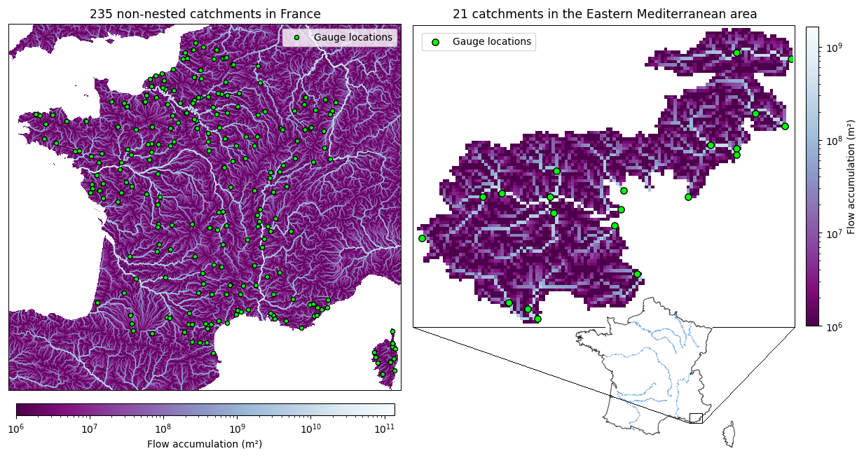
Figure 2 Study areas used for evaluation. The first area consists of 235 non-nested catchments in France, while the second area includes 21 catchments in a multi-catchment setup in the eastern Mediterranean region representing contrasting hydrological conditions.

The SMASH model is run on a spatial grid with a resolution of dx=1 km and a temporal step of dt=1 h. It is forced by the following data:

• Discharge. This is collected by the French Ministry of the Environment, covering the period of the forcing data and extracted from the HydroPortail platform (http://www.hydro.eaufrance.fr, last access: 1 August 2025).

• Rainfall. We use rainfall data from the ANTILOPE J+1 radar observation reanalysis, which merges radar data with in situ gauge observations. These data are provided by Météo-France at a grid resolution of 1 km², matching the resolution of the model grid rasters.

• Potential evapotranspiration (PET). Temperature data for calculating PET are sourced from the SAFRAN (Système d'Analyse Fournissant des Renseignements Atmosphériques à la Neige) reanalysis, provided by Météo-France at a resolution of 8 km×8 km (Quintana-Seguí et al., 2008; Vidal et al., 2010). The PET is then computed using the Oudin formula (Oudin et al., 2005) and has the same resolution as the rainfall data.

The first dataset contains hourly time series over a 13-year period (August 2006 to July 2019) for downstream gauges only. It is used to evaluate single-gauge optimization (local calibration) without regionalization, focusing solely on the process-parameterization neural network ϕ₁, which is the key novelty of this study. The 13-year period is divided into two segments: the calibration period covers the first 7 years (including a 1-year warmup), and the remaining 6 years are used for temporal validation. Four methods are compared to evaluate the learning capacity of the neural network ϕ₁:

• Two classic GR models with spatially uniform parameters (GR.U) and spatially distributed parameters (GR.D), which, in some cases, exhibit under-parameterization or over-parameterization issues in the spatially distributed hydrological model

• Two hybrid GR models that integrate the neural network ϕ₁ (called ϕ₁-hybrid) with spatially uniform parameters (GRNN.U) and spatially distributed parameters (GRNN.D)

The second dataset includes hourly time series over 7 years (August 2009 to July 2016) for both nested and independent catchments in the eastern Mediterranean region (known as “MedEst”). This dataset is used to assess the relevance of the learnable structure for simultaneous multi-gauge regionalization with physical descriptors. A set of seven descriptors (Table A1 and Fig. A1 in Appendix A), with a spatial resolution of 0.01° in the WGS84 projection and encompassing various types such as topography, morphology, land use, and hydrogeology, is used as input for the regionalization mapping ϕ₂. The MedEst region presents a challenging case due to its contrasting hydrological properties, including steep topography and highly heterogeneous soils and bedrock (e.g., Garambois et al., 2015). This region is prone to intense rainfall events that trigger nonlinear flash flood responses and contains a significant proportion of karstic zones. The first 4-year time series, including a 1-year warmup period, is used for calibration, while the remaining 3 years are used for validation. Four methods are compared to evaluate the learning capacity of both the process-parameterization neural network ϕ₁ and the regionalization neural network ϕ₂:

• the classical GR model with regional, spatially uniform parameters (GR.U);

• the hybrid GR model integrating the neural network ϕ₁ (ϕ₁-hybrid) to correct internal fluxes in hydrological processes, with regional, spatially uniform parameters (GRNN.U);

• the classical GR model integrating the neural network ϕ₂ (ϕ₂-hybrid) to learn the mapping between physical descriptors and spatially distributed hydrological parameters (GR.NN); and

• the hybrid GR model integrating both neural networks ϕ₁ and ϕ₂ (GRNN.NN), representing the fully integrated hybrid approach (ϕ-hybrid) among the studied methods.

While the first dataset aims to test the performance of the neural network ϕ₁ in flux correction using local calibrations only at downstream gauges over Metropolitan France, the second aims to evaluate regional calibration in a multi-catchment setup, testing the performance of both ϕ₁ (for process parameterization) and ϕ₂ (for regionalization). Note that performing a global multi-catchment calibration (e.g., at the national scale across the entire mesh of France) for process parameterization and regionalization with neural networks is computationally challenging given the high spatiotemporal resolution of the data and model. In this study, we focus on a specific and well-known study zone. It is worth mentioning that regionalization performance (without a process-parameterization network) over a larger zone, covering approximately one-fourth of France, was already investigated in Huynh et al. (2024b). Future work could extend this study to a national-scale multi-catchment setup.

4 Results and discussion

In this section, we first present the performance of the hybrid spatially distributed models tested on both datasets. Then, we will provide further interpretation and discussion of the learning process to analyze the proposed framework and enhance the understanding of hydrological behaviors in the process-based model through internal fluxes.

4.1 Model performance analysis

4.1.1 Local calibration over 235 French catchments

Figure 3 illustrates typical simulated streamflows from different methods for small, medium, and large catchments. Overall, we observe significant improvements in the hybrid methods compared to the classical models in simulating both peak flows and low flows. For example, in the case of the medium catchment, GRNN.U more accurately predicts the peak flows in January 2014 compared to GR.U while also reliably reproducing the low flows, particularly during the period between 2018 and 2019.

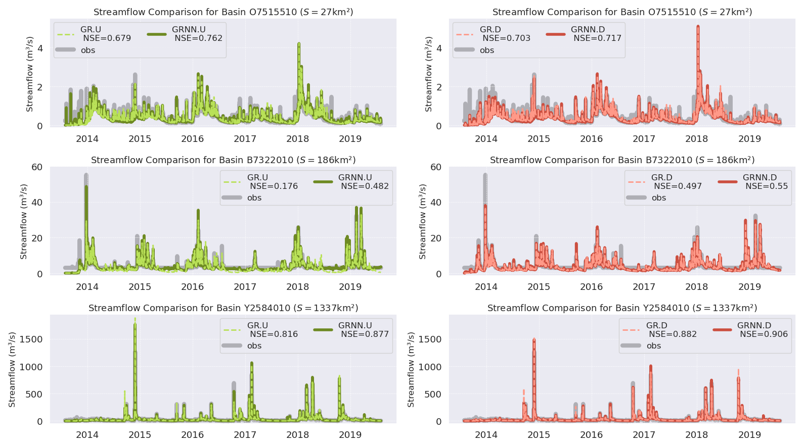
Figure 3 Comparison of streamflow simulation across representative small, medium, and large catchments randomly selected from the 235 catchments in France during the validation period.

Figure 4 shows a global comparison of performances in terms of Nash–Sutcliffe efficiency (NSE), Kling–Gupta efficiency (KGE), and root mean squared error (RMSE) across both calibration and validation periods for the different methods. The results suggest that the ϕ₁-hybrid methods (GRNN.U and GRNN.D) consistently achieve superior efficiency scores and lower errors compared to the classic models (GR.U and GR.D) in various scenarios. In calibration, both hybrid models outperform the classical ones, with significantly higher median NSE scores (0.85 and 0.86 compared to 0.79 and 0.83), a narrower and higher interquartile range, and a shorter lower whisker.

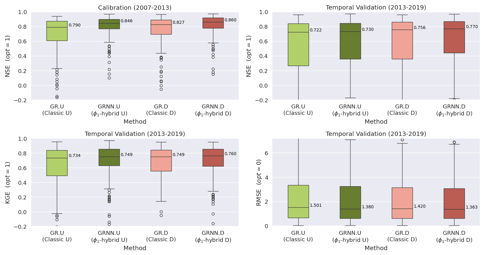
Figure 4 Model performance comparison of local calibration methods across 235 catchments in France. The two boxes in lighter colors represent the classical GR models (GR.U and GR.D), while the two boxes in darker colors represent the ϕ₁-hybrid models (GRNN.U and GRNN.D). The evaluation is based on simulated discharges over the calibration and validation periods, using NSE, KGE, and RMSE metrics.

In temporal validation, GRNN.U achieves a median NSE of 0.73 compared to 0.76 for GR.D, and both models reach a median KGE of 0.75, while GRNN.U shows a lower median RMSE of 1.38 compared to 1.42 for GR.D. Although median improvements may appear small, it is important to consider the entire distribution. In addition to the median values, we observe notable enhancements in other statistical measures, such as the interquartile range (0.25 and 0.75 quantiles) and whiskers in the boxplots. For catchments that already exhibit satisfactory performance, the effect of hybridization is relatively small, leading to similar median 0.75 and 0.95 quantile values. However, for poorly performing basins, the hybrid models provide substantial improvements, as evidenced by enhanced performance in the lower quartiles. Notably, the hybrid model with spatially uniform hydrological parameters (GRNN.U) performs comparably to, and in some cases surpasses, the classic GR model with spatially distributed parameters (GR.D). This result is promising, as it demonstrates that, while the original model with spatially uniform conceptual parameters (GR.U) inherently leads to under-parameterization compared to GR.D, this limitation can be compensated for by the spatially distributed flux correction in GRNN.U.

To evaluate flood simulation performance, Huynh et al. (2023) introduced a method to compute several flood event signatures using an automatic segmentation algorithm. These signatures help depict the model behavior during flood events. Relative error is used as the evaluation metric to quantify the difference between simulated and observed flood event signatures, including peak flow, runoff coefficient, flood flow, and baseflow. Figure 5 shows the cumulative distribution function (CDF) of the relative error for these signatures, based on over 2700 flood events that occurred during the 6-year validation period. The hybrid models achieve the best performance, outperforming the classical GR.U model, with their CDF lines consistently above. Notably, the hybrid model GRNN.U, using only spatially uniform parameters, attains a performance comparable to or even better than the classical model with spatially distributed parameters (GR.D). GRNN.U shows similar performance to GR.D in reproducing peak flows (with the same median error of 0.32) and flood flow (both with a median error of 0.28) while performing slightly better in reproducing the runoff coefficient (0.20 compared to 0.22) and baseflow (0.21 compared to 0.22). This highlights the strength of the hybrid process-parameterization framework, particularly its relevance in improving flood modeling systems.

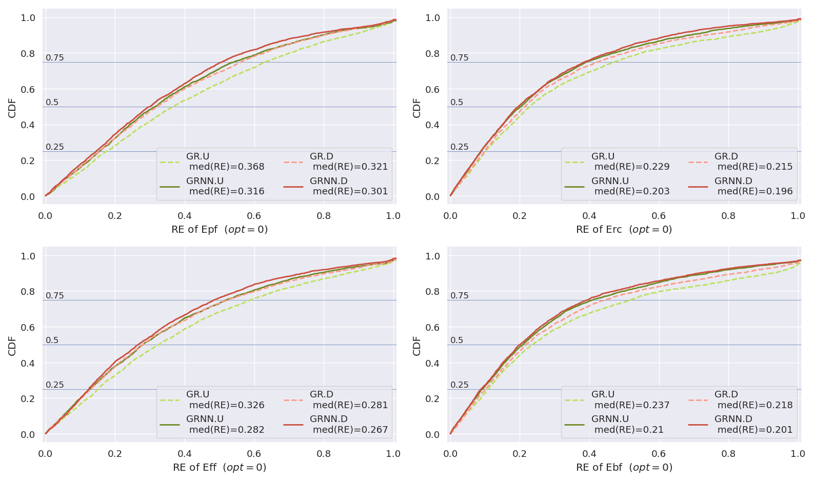
Figure 5 Comparison of model performance in simulating flood event signatures, presented as the cumulative distribution function (CDF) of the relative error (RE) between observed and simulated values for peak flow (Epf), runoff coefficient (Erc), flood flow (Eff), and baseflow (Ebf). The evaluation is based on 2718 flood events across 235 catchments during the validation period (August 2013–July 2019).

4.1.2 Multi-catchment regionalization over a flash-flood-prone Mediterranean area

Here, we investigate how the hybrid models perform in a study of a multi-catchment regionalization setup. In calibration, it is evident from Fig. 6 that the ϕ₂-hybrid model (GR.NN) and the ϕ-hybrid (GRNN.NN) model, both using the regionalization neural network ϕ₂, outperform the models with lumped parameters (GR.U and GRNN.U). Notably, the fully integrated hybrid model GRNN.NN dominates the radar plot, with a large shape extending toward the outer edges and fully enveloping the other methods. Although GRNN.U clearly falls short of the two regionalization-based models, it still shows a significant improvement over the classic GR.U model. Similar results can be observed in both temporal and spatiotemporal validation, as seen in the boxplots. This proves that using physical descriptors with learnable mapping is an effective approach in this regionalization setup (multiple catchments in a large, flash-flood-prone area with high-spatiotemporal-resolution data) compared to lumped models (without physical descriptors) or simpler regionalization methods (e.g., multilinear or multi-polynomial mappings), as demonstrated in Huynh et al. (2024b). Interestingly, while the ϕ-hybrid model GRNN.NN, which delivers the best overall performance, shows a moderate gain over GR.NN – with median NSE scores of 0.75 (compared to 0.72) and 0.51 (compared to 0.48) in temporal and spatiotemporal validation – the ϕ₁-hybrid model GRNN.U, which uses lumped parameters without regionalization using physical descriptors, is a dramatic improvement over the classic GR.U model (median NSE values of 0.56 compared to 0.14 and 0.43 compared to 0.16). In this way, learning internal flux corrections has made it possible to improve the regionalizability of a distributed conceptual hydrological model, even with spatially uniform conceptual parameters (i.e., without using physical descriptors). This may represent a compelling research direction for reducing structural uncertainty in modeling, using a minimum of data and enabling more efficient extraction of multiscale information through hybrid flux correction with GRNN.U, with the potential for flexible semi-spatializations of conceptual parameters and even proximity-based regionalizations for spatially dense gauging networks (cf. Oudin et al., 2008).

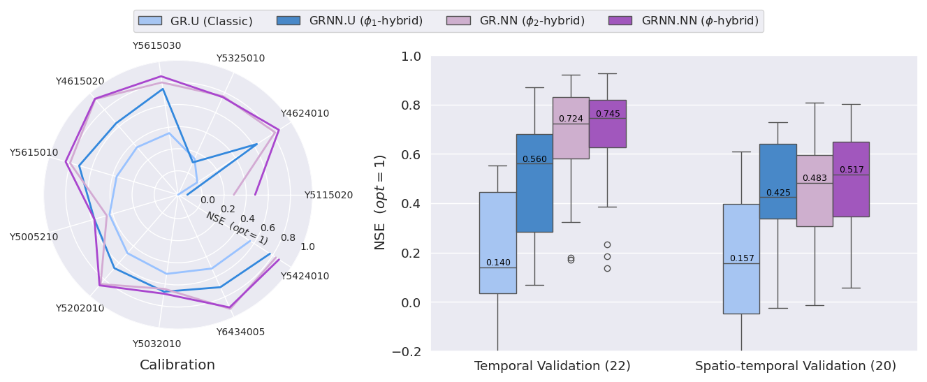
Figure 6 Comparison of multi-catchment regionalization performances for different methods. The evaluation is based on NSE scores computed over three periods: the 3-year calibration period (excluding a 1-year warmup), the first 18 months, and the last 18 months of the 3-year validation period for 11 calibration catchments and 10 validation catchments. The numbers in parentheses in the boxplots indicate the total number of samples evaluated, with the validation period split into two 18-month periods (sample counts are doubled for all of the catchments).

In the context of flood prediction, the hybrid models (GRNN.U, GR.NN, and GRNN.NN) consistently yield superior performance compared to the classical GR.U model. Figure 7a presents the RMSE and NSE metrics computed using short time series from 143 flood events that occurred across the entire MedEst area during the validation period from August 2013 to July 2016 (similar graphs for additional evaluation metrics are shown in Fig. B5 in Appendix B). Figure 7b shows typical streamflow simulations, demonstrating a significant enhancement for both hybrid process-parameterization and regionalization-based approaches, compared to classical methods, in simulating high flow characteristics and behaviors during flood events.

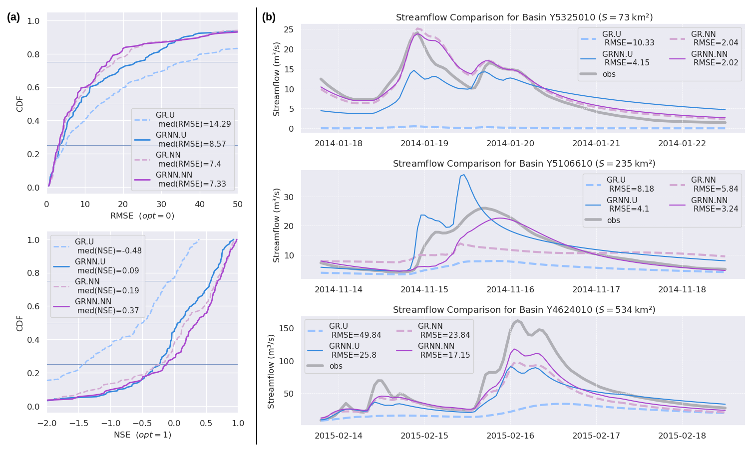
Figure 7 (a) Comparison of NSE and RMSE metrics computed for 143 flood events detected in the validation period across 21 catchments in the MedEst region. (b) Comparison of streamflow simulations for representative small, medium, and large catchments during several flood events selected in the validation period.

Although the NSE values computed for the 143 flood events are relatively low across all of the models, it is important to note that the NSE for flood events – which are short time series with high values – is highly sensitive to small timing errors. Even slight discrepancies in peak timing can lead to substantial decreases in NSE. Additionally, data and modeling uncertainties may vary between events, making accurate prediction of highly contrasted events particularly challenging. The models are calibrated on the entire time series, and we evaluate the validation results specifically for flood events, where classical approaches often struggle to accurately estimate water dynamics. This discrepancy highlights the difficulty in capturing the rapid and intense nature of flood events, even with advanced hybrid models and simplified hydraulic routing. This underscores the need to investigate potential sources of error, including input data quality and model structural limitations, as well as the impact of using a calibration metric based solely on flood events. These factors could explain the overall challenges in flood event simulation.

4.2 Towards learning hydrological behaviors

Here, we focus on uncovering the hydrological behaviors inferred with the hybrid approach, consisting of neural networks embedded in a physical model for learnable correction of internal fluxes. In the studied hybrid structure GRNN, the learned correction of GR-like model consists of four flux corrections ${\mathit{f}}_q(x,t)={\left(f_{q,i}(x,t)\right)}_{i=\mathrm{1}\mathrm{\dots }\mathrm{4}}={\mathit{\varphi }}_{\mathrm{1}}(P_{\mathrm{n}},E_{\mathrm{n}},h_{\mathrm{p}},h_{\mathrm{t}})(x,t)$ for each pixel and time step of the simulation domain from atmospheric forcings and previous model states. A positive (or negative) correction of f_q,i (where $i=\mathrm{1},\mathrm{2},\mathrm{4}$), with values bounded in $]-\mathrm{1};\mathrm{1}[$ due to the TanH activation function used in the output layer, results in an increase (or decrease) in the original fluxes P_s, E_s, and $\left|F\right|$ – the absolute value of F (cf. Eqs. 4, 5, and 7), thereby influencing the simulated mass balance. Meanwhile, $f_{q,\mathrm{3}}^{\mathrm{2}}$, with values in [0;1[, produces a conservative re-repartitioning of the net rainfall P_r between direct and delayed transfer branches (cf. Eq. 6), thereby affecting the subgrid transfer dynamics. The following quantitative analysis begins with the spatiotemporal averages of these flux corrections and proceeds to explore their variability across the 235 independently calibrated catchments, as well as in the regionalization test case.

4.2.1 Analysis of internal flux corrections

Figure 8 shows the maps of spatiotemporal average flux corrections (the corrections are first averaged spatially within each catchment and then temporally across the calibration period), obtained through local calibrations using GRNN.U (see Fig. B1 in Appendix B for GRNN.D). Red and blue indicate positive and negative flux corrections in the spatiotemporal average. For fluxes affecting the production reservoir, i.e., infiltrating rainfall P_s and evapotranspiration E_s, the average corrections show opposite signs for the majority of the basins and the same sign for a minority. These maps reveal different trends of flux corrections across France. Several regions exhibit strong corrections (either negative or positive) for P_s and E_s, while others show near-zero corrections (white points with values close to 1). However, the exchange flux is generally the one most influenced by the corrections, as indicated by the dark colors across the maps, playing a crucial role in refining the model's state dynamics. Note that the transformation function $\mathrm{1}-f_{q,\mathrm{3}}^{\mathrm{2}}$ applied to correct the delayed transfer flux Q_dl results in a reduction of this flux and conservative augmentation of the Q_dr flux feeding the direct branch.

Figure 8 Maps of spatiotemporal average flux corrections ${\stackrel{\mathrm{‾}}{{\stackrel{\mathrm{‾}}{g\left({\mathit{f}}_q\right)}}^{x\in {\mathrm{\Omega }}_j}}}^t$, where j=1…N_g for the N_g=235 catchments obtained through local calibrations of spatially uniform parameters with the hybrid model structure (GRNN.U). The function g(.) represents the transformation applied to the neural network output f_q, which may differ depending on the specific flux being corrected. Red indicates corrections that tend to increase the current flux, while blue indicates corrections that reduce it, with white representing minimal or no effective correction.

Now, we turn to the analysis of the time series of the spatially averaged flux corrections presented in Fig. 9 (see Fig. B2 for GRNN.D). Figure 9a illustrates these corrections over time for 3 randomly selected catchments that are representative of the 235 French catchments (corresponding results for all 235 catchments are provided in Fig. B4). We observe opposite signs in the corrections f_q,1 and f_q,2 for infiltration P_s and evapotranspiration E_s from the production reservoir. Catchments exhibiting positive corrections to P_s and negative corrections to E_s suggest that more water is directed towards the production reservoir and that less is lost by evapotranspiration, leading to an increased moisture state. Conversely, in catchments with negative corrections for P_s and positive corrections for E_s, reduced infiltration and increased evapotranspiration imply lower moisture states. Furthermore, periodic behaviors are observed over time for corrections of the four water fluxes, highlighting the temporal patterns of flux corrections. This pattern likely reflects the footprint of the annual periodicity of the production state h_p, which is an input to the neural network ϕ₁. Overall, the corrected infiltrating rainfall ${\stackrel{\mathrm{̃}}{P}}_s$ is generally 10 % higher than the original, as indicated by the median of $\mathrm{1}+f_{q,\mathrm{1}}$ being approximately 1.10 in Fig. 9b. This implies an increased water level in the production reservoir and hence more water being directed there rather than feeding the transfer branch. This observation somehow explains why the production capacity c_p, calibrated for the hybrid models, is generally slightly higher than that of the classical models (see Table B1 in Appendix B). Additionally, fewer corrections are obtained for re-repartitioning of the net rainfall flux into the direct and delayed transfer branches (i.e., the corrections show less variation and are closer to 1). Negative corrections that tend to reduce the flux magnitude are applied to the delayed transfer branch ${\stackrel{\mathrm{̃}}{Q}}_{\text{dl}}$, which implies positive corrections for the direct transfer branch ${\stackrel{\mathrm{̃}}{Q}}_{\text{dr}}$. In this case, the hybrid model suggests that more water reaches the outflow Q_rd via the direct transfer branch. Both transfer branches are affected by the exchange flux $\stackrel{\mathrm{̃}}{F}$ for which, across most catchments, a reduction is obtained by flux correction (the median of $\mathrm{1}+f_{q,\mathrm{4}}$ is lower than 1).

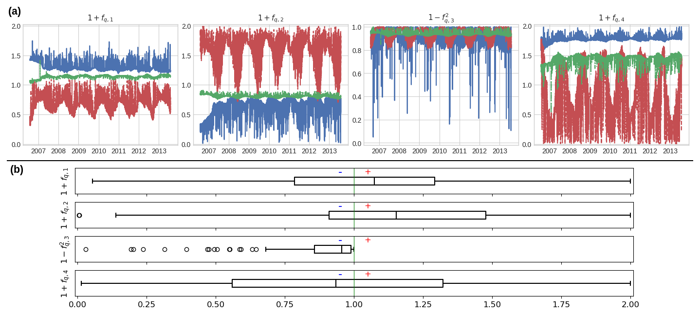
Figure 9 (a) Spatially averaged flux correction time series ${\stackrel{\mathrm{‾}}{g\left({\mathit{f}}_q\left(t\right)\right)}}^{x\in {\mathrm{\Omega }}_j}$ for 3 randomly selected catchments from the set of 235. These are obtained through local calibrations of spatially uniform parameters with the hybrid model structure (GRNN.U). (b) Boxplot of spatiotemporal average flux corrections ${\stackrel{\mathrm{‾}}{{\stackrel{\mathrm{‾}}{g\left({\mathit{f}}_q\right)}}^{x\in {\mathrm{\Omega }}_j}}}^t$, where each boxplot represents 235 catchment-specific spatiotemporal averages.

In a multi-gauge regionalization setup, distinct spatiotemporal patterns emerge over the MedEst area, as shown in Fig. 10 for GRNN.U (corresponding results for GRNN.NN are shown in Fig. B6 in Appendix B). Figure 10a illustrates that the spatially averaged corrections for infiltrating rainfall P_s show relatively high temporal variability; moreover, they still exhibit stable periodic patterns after the first year of warmup. The spatial average of the corrected flux ${\stackrel{\mathrm{̃}}{P}}_s$ tends to be lower during moderate-rain events, while it is higher during high-rain events compared to the original flux P_s. This suggests that the hybrid model directs more rainfall into the transfer branch during moderate-rain events (which may have longer durations), while the opposite behavior is observed for high-rain events (which can be shorter in duration). The spatial maps of time-averaged flux corrections in Fig. 10b further indicate that the hybrid model generally applies negative corrections, reducing the spatiotemporal mean of infiltrating rainfall from 0.1 mm to 0.06 mm. Interestingly, these maps also reveal spatial variability in internal flux corrections, which may explain the improved regionalizability of the hybrid GRNN models, as demonstrated by their performance in spatiotemporal validation, even with spatially uniform conceptual parameters (without regionalization using physical descriptors). While temporal patterns of flux corrections (e.g., annual periodicity) emerge from the production and transfer states, similar to the case of the 235 catchments, spatial patterns are likely due to the spatial variability of atmospheric data.

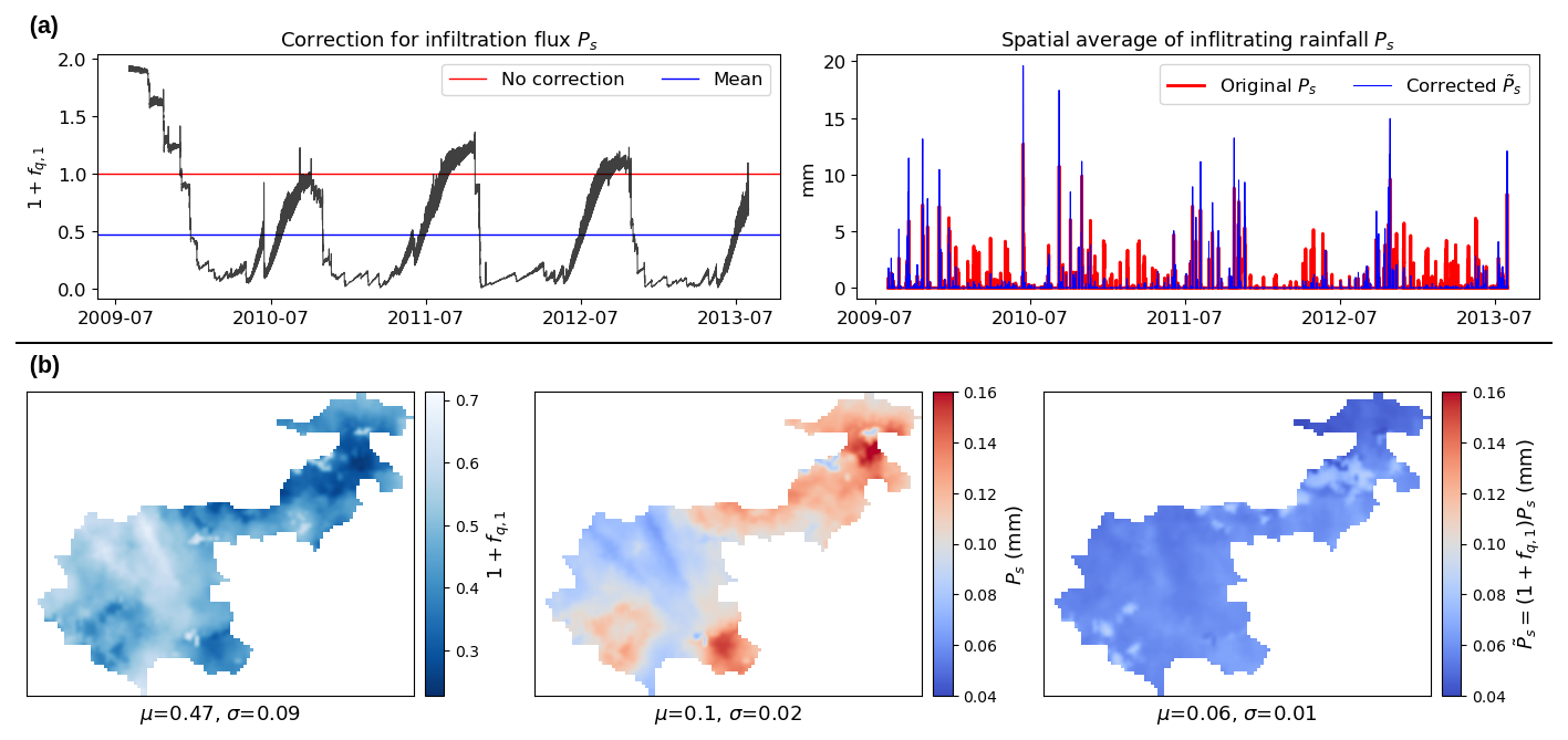
Figure 10 Visualization of flux corrections in the MedEst region obtained through regional calibration of spatially uniform parameters with the hybrid model (GRNN.U). (a) Spatial average of the infiltrating flux correction ${\stackrel{\mathrm{‾}}{\mathrm{1}+f_{q,\mathrm{1}}\left(t\right)}}^x$, original rainfall ${\stackrel{\mathrm{‾}}{P_s\left(t\right)}}^x$, and corrected infiltrating rainfall ${\stackrel{\mathrm{‾}}{{\stackrel{\mathrm{̃}}{P}}_s\left(t\right)}}^x$. (b) Maps of the time-averaged infiltrating flux correction ${\stackrel{\mathrm{‾}}{\mathrm{1}+f_{q,\mathrm{1}}\left(x\right)}}^t$, original rainfall ${\stackrel{\mathrm{‾}}{P_s\left(t\right)}}^x$, and corrected infiltrating rainfall ${\stackrel{\mathrm{‾}}{{\stackrel{\mathrm{̃}}{P}}_s\left(x\right)}}^t$, where μ and σ represent the spatial average and standard deviation.

4.2.2 Hybridization effect on the main mass fluxes involved in a basin's water balance

This section examines the effect of ϕ₁ hybridization on the primary mass fluxes involved in the hydrological mass balance, as simulated using the original GR-like spatially distributed model structure. For a given catchment domain Ω, the annual catchment-scale flux Ψ_f,𝒜 of a state flux f(x,t) – such as actual evapotranspiration, exchange flux, or runoff flux – simulated using either the classical model or the hybrid model (with flux corrections omitted for brevity) is computed as follows:

$$\begin{array}{}\text{(13)}& {\displaystyle }{\displaystyle }{\mathrm{\Psi }}_{f,\mathcal{A}}={\displaystyle \frac{\mathrm{1}}{\left|\mathrm{\Omega }\right|}}\underset{t\in \mathcal{A}}{\int }\underset{x\in \mathrm{\Omega }}{\int }f(x,t)\mathrm{d}x\mathrm{d}t,\end{array}$$

where 𝒜 denotes the annual period and $\left|\mathrm{\Omega }\right|$ represents the drainage area.

A basin-scale analysis is performed for each of the 235 French basins simulated, focusing on the flux of rainfall P inflowing into the model and three key fluxes affected by the ϕ₁ hybridization: evapotranspiration E_s from the production store, exchange F, and the pixel-scale discharge Q_lat prior to routing. The annual average of each flux is calculated using Eq. (13), and the interannual averages of these water gain or loss fluxes over the 6-year calibration period (2007–2013) are shown in Fig. 11. This figure quantitatively illustrates the impact of ϕ₁ hybridization on the classical GR-like model, with uniform conceptual parameters for each basin and each model structure. Of the variety of hydrological behaviors and annual rainfall regimes of this large catchment set, it is noteworthy that hybridization results show almost no change for nearly all basins in terms of interannual discharge runoff volume, with medians of 246.6 mm for GR.U and 251.3 mm for GRNN.U and similar quantiles, while dynamic changes have been obtained as suggested by the improved NSE, flood signatures, and hydrographs (cf. the performance analysis in Sect. 4.1) as well as internal flux corrections (such as infiltration and repartitioning between direct and delayed lateral transfer branches).

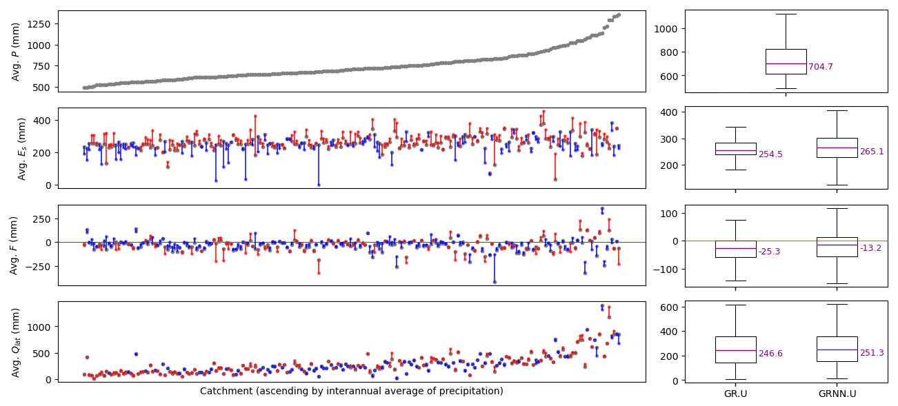
Figure 11 Comparison of mass fluxes affecting water balance in the interannual mean at the basin scale over the 235-catchment set for the classical GR model (GR.U) and the ϕ₁ hybrid model (GRNN.U) using uniform mapping “U” for conceptual parameters θ in local calibration. The x axis shows the 235 catchments, sorted by their average precipitation. The grey dots represent the interannual averages of precipitation P, actual evapotranspiration E_s, exchange flux F, and lateral discharge Q_lat over the calibration period for the classical model. The red dots and lines represent increases according to the hybrid model, while the blue ones indicate decreases. For cases where F<0, red indicates a larger magnitude in F for the hybrid model (more negative), while blue indicates a lesser magnitude (closer to 0).

The simulated water balance is influenced by the correction of k_exc, which represents the exchange flux and can result in either gains or losses relative to the original model (which is already nonconservative). In this case, the exchange flux is moderately affected by hybridization, with a median trend of reduced exchange from −23.5 to −13.2 mm. This reduction is compensated, in terms of water balance, by an increase in evaporation from the production reservoir (from 254.5 to 265.1 mm in the median). Notably, both fluxes exhibit a larger interquartile range across basins compared to the classical model structure. Therefore, the proposed ϕ₁ hybridization enables learning of spatiotemporal corrections of internal model dynamics, resulting in physically interpretable fluxes that remain within imposed ranges and lead to overall model improvement.

Figure 12 depicts the versatile nature of the learnable hybrid model in comparison to classical conceptual models for correcting internal fluxes and vividly illustrates the learned nonlinear relationship between the corrected net rainfall and neutralized data, together with the internal states. The model response surface of the net rainfall $P_{\mathrm{r}}=P_{\mathrm{n}}-\stackrel{\mathrm{̃}}{P_s}$, obtained with the corrected infiltrating rainfall ${\stackrel{\mathrm{̃}}{P}}_s=(\mathrm{1}+f_{q,\mathrm{1}})P_s$, is shown for different levels of the production state h_p and neutralized rainfall P_n. Interestingly, this corrected net rainfall $P_{\mathrm{n}}-\stackrel{\mathrm{̃}}{P_s}$, regardless of the level of the production state (i.e., $h_{\mathrm{p}}=\mathrm{0.3},\mathrm{6}$, and 15 mm), exhibits nonmonotonic behavior with respect to the intensity of neutralized rainfall P_n (Fig. 12a). However, this nonmonotonic behavior becomes less pronounced as the production state h_p approaches the production capacity c_p. Figure 12b further clarifies the nonlinear response surface, showing that the corrected net rainfall undergoes two changes in monotonicity as the neutralized rainfall when the reservoir is less than half-utilized ($h_{\mathrm{p}}<c_{\mathrm{p}}/\mathrm{2}$). In contrast, when the reservoir is fully or nearly fully utilized (h_p≈c_p), the corrected flux $P_{\mathrm{n}}-{\stackrel{\mathrm{̃}}{P}}_s$ behaves similarly to the original flux P_n−P_s. Interestingly, nonlinear infiltration behavior is obtained after learning with the hybrid GRNN model structure, especially for drier conditions of the production reservoir where classical GR models are known to fail in flood generation (cf. Astagneau et al., 2021). Further research could focus on deeper analysis of learned physical behaviors, e.g., by investigating the approximation of learned behaviors with known mathematical functions. One could also investigate how to a priori directly impose physically onto the forward model structure using other mathematical expressions, e.g., imposing a explicit monotonicity or even a shape of dependency, such as the rainfall-intensity-related modifications of the original lumped GR model in Astagneau et al. (2022).

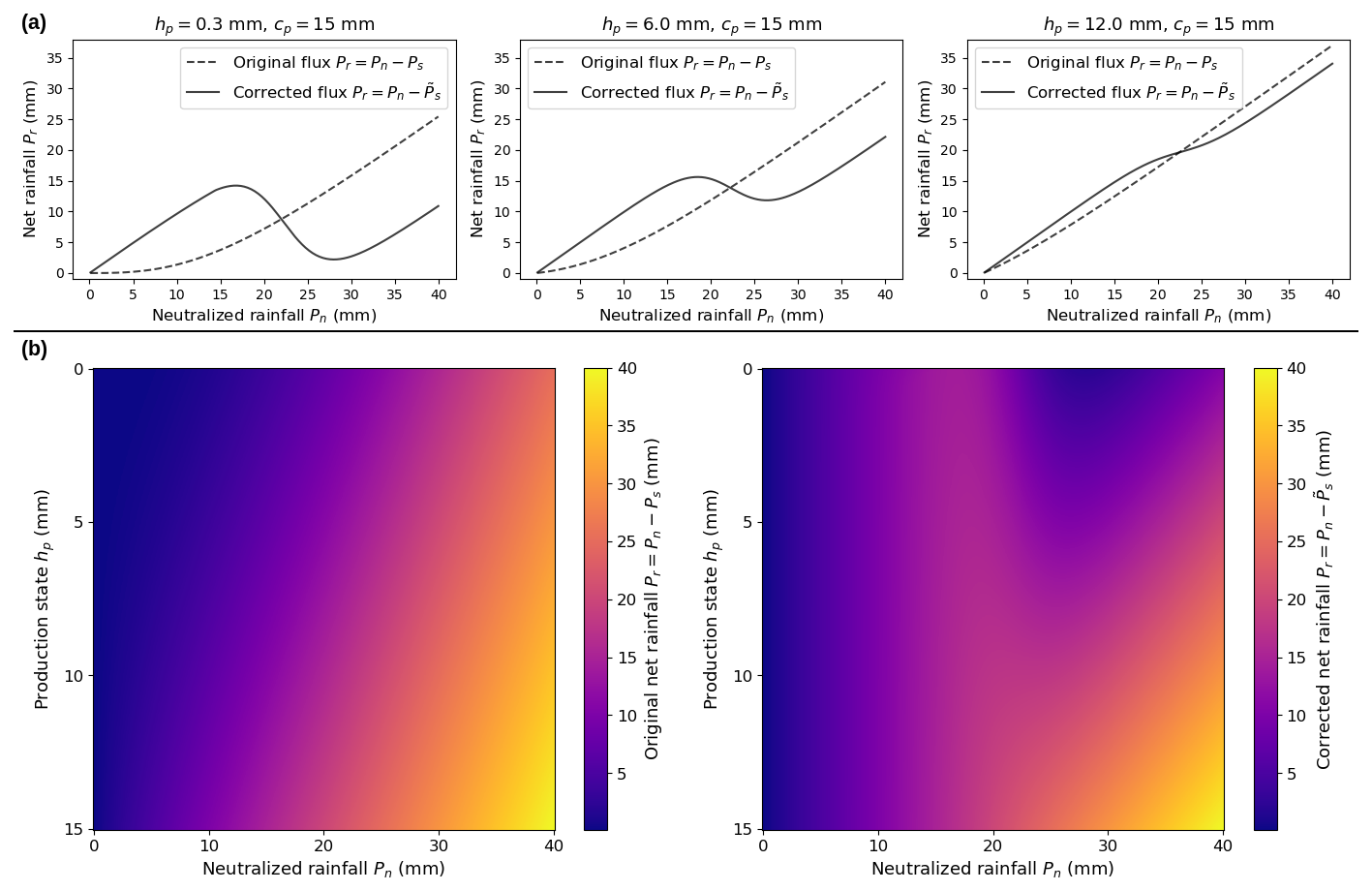
Figure 12 Hydrological interpretation of the nonlinear response surface obtained using the learned flux correction neural network for infiltrating rainfall ${\stackrel{\mathrm{̃}}{P}}_s=(\mathrm{1}+f_{q,\mathrm{1}})P_s$, plotted with a production capacity of c_p=15 mm and a neutralized evapotranspiration of E_n=0 mm. (a) Original and corrected net rainfall P_r for different levels of the production state h_p. (b) Response surface of the original and corrected net rainfall P_r as a function of both the production state h_p and neutralized rainfall P_n.

4.3 Research perspectives and further discussion

This article proposed a spatially distributed hybrid GR-like model and a comprehensive analysis of a large catchment sample. Future research should concentrate on refining the model's hybridization strategy in order to enhance its applicability across even larger datasets (e.g., the CARAVAN database in Kratzert et al., 2023) and to improve extrapolation capabilities for extreme hydrometeorological events. This quest for generalized structures of spatially distributed hydrological models requires scalable hybrid solvers applicable over very large domains. Immediate work will focus on developing a SMASH version for parallel GPU-based forward-inverse computation and adapting the ϕ-hybrid model to a state space GR model (cf. Santos et al., 2018), thereby enabling the investigation of additional nonlinearities in hydrological model differential equations. In addition, improving the routing model may deliver a more realistic flood wave propagation. Such improvement could be based on the use of known hydraulic models (e.g., kinematic wave in Roux et al., 2011, and Vergara et al., 2016, non-inertial 1D or 2D in Fleischmann et al., 2020, or full 1D Saint-Venant at the network scale in Larnier et al., 2025), fine topography data such as lidar obtained during low flows (capturing a significant part of the river bathymetry), and/or more observations of flow depth, extent, and velocity.

Although hybrid models have more degrees of freedom compared to classical GR models, it is important to note that the inputs and outputs of the flux correction model are physically consistent and of the same dimension as the original model. This design allows the hybrid model to learn nonlinearities in the internal flux laws, which we analyze thoroughly in the flux correction analysis in both time and space throughout the paper. The hybrid models do not necessarily have more conceptual parameters (maintaining the same number of reservoirs and connections here), but they do introduce more nonlinearity into the internal flux law corrections with the neural network ϕ₁. This added complexity effectively increases the model's degrees of freedom while maintaining robustness in both spatial and temporal validations, as demonstrated by the numerical results.

It is worth noting that the two neural networks will not be extrapolated in the same way when the model is used in prediction. The regionalization neural network ϕ₂ will not be extrapolated as long as the model is used in the region in which it has been calibrated. At the opposite end, the flux correction neural network ϕ₁ is bound to be extrapolated since its inputs $(P_{\mathrm{n}},E_{\mathrm{n}},h_{\mathrm{p}},h_{\mathrm{t}})$ vary in time, so that the range observed in the calibration will be exceeded sooner or later. This is particularly the case when the model is calibrated locally, as done in the first case study involving 235 French catchments. By contrast, a multi-catchment regionalization setup (Mediterranean case study) is advantageous since it offers more opportunity to expose ϕ₁ to extreme values of its inputs. Quantifying the uncertainty affecting the estimated parameters of the neural networks would be useful for raising awareness of a likely loss of precision when ϕ₁ is extrapolated, but this comes with many difficulties (e.g., Papamarkou et al., 2022). An alternative approach would be to look for parsimonious regressions that are able to adequately reproduce the behavior revealed by ϕ₁ while being amenable to uncertainty quantification.

Finally, the proposed hybrid hydrological framework should be extended to other model structures, as with the other GR or variable infiltration capacity (VIC) available on the SMASH platform, but it should also use more complex physics-based modeling approaches and hypothesis testing such as in Douinot et al. (2018) with various subsurface flow models. Note that the proposed physics–AI framework for spatially distributed modeling could help unify top–down approaches such as GR or other data-based conceptual models with bottom–up physics-based hydrological models that suffer from (up)scaling problems of physical laws and parameterization. In the context of relatively sparse discharge data compared to model dimensionality, such a model discovery process could greatly benefit from the wealth of surface information provided by remote sensing. This includes data on terrain and vegetation properties, surface moisture, snow cover, surface temperature, and total water storage (Meyer Oliveira et al., 2021) along with river network data (e.g., river flow surface topography variability through altimetry and imagery), which necessitates a differentiable river network hydraulic model to achieve coherence with hydraulic observables while enabling the inference of complex and large spatiotemporal parameters from heterogeneous data (Larnier et al., 2025). Such a model would also support information feedback from these data to the hydrological model within a differentiable H&H coupling framework (Pujol et al., 2022).

5 Conclusions

This article introduces a hybrid physics–AI framework that integrates neural networks to infer spatiotemporal internal fluxes and spatially distributed conceptual parameters within a differentiable, gridded hydrological model, all encapsulated in a VDA algorithm. Numerical results from local calibration and validation across 235 French catchments and regionalization in a complex, flash-flood-prone area demonstrate the superiority of the hybrid models. These models excel not only in performance scores during both calibration and validation but also in producing physically interpretable results, with improved representations of simulated hydrological behavior.

The proposed approach, relying on process-based equations hybridized with ANNs, allows interpretable spatially distributed hydrological models to be obtained, in contrast to pure machine learning approaches, while taking advantage of nonlinear and multiresolution effects of neural networks. Accordingly, it is applicable to any other differentiable hydrological, hydraulic, or geophysical model on structured or unstructured meshes.

Future work will aim to enhance the hybrid framework by (i) studying the generalizability of structural corrections across larger datasets and diverse model structures; (ii) investigating more complex neural networks, including deeper ANNs, to capture multiscale information over larger datasets in global optimization or simpler tools that could reproduce the behavior revealed by the ANNs while facilitating uncertainty quantification; (iii) exploring mathematical properties, such as equifinality issues between neural networks and conceptual parameters, and analyzing the response surfaces of universal differential equation sets for flexible hydrological modeling in time and space; and (iv) coupling with differentiable river network hydraulic models to improve 1D–2D hydrodynamic realism. This coupling will enable feedback by assimilating hydraulic observations into a differentiable H&H chain (Pujol et al., 2022), such as the unprecedented hydraulic visibility (Garambois et al., 2017) brought by SWOT (Surface Water and Ocean Topography) and multi-satellite data (e.g., with VDA in Pujol et al., 2020, and Malou et al., 2021). Such differentiable and learnable H&H modeling frameworks are expected to enhance the representation of basin-internal state fluxes and enable efficient fusion of machine learning with process-based modeling, advancing the discovery of scale-relevant hydrological laws through maximal extraction of information from multisource data.

Appendix A: Input physical descriptors for learning regionalization

Table A1 and Fig. A1 provide information on the physical descriptors used as input data for regionalization learning methods. Note that, before the optimization process, all descriptors are standardized between 0 and 1 using min–max scaling.

Odry (2017)Organde et al. (2013)Arnaud et al. (2014)Agency (2019)Agency (2019)Poncelet (2016)Finke et al. (1998)

Table A1 Descriptors used as input data for regionalization methods.

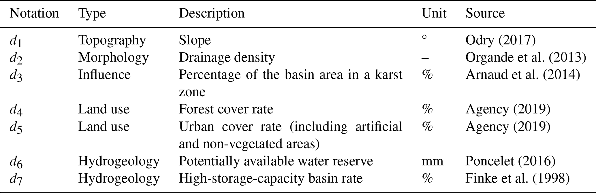
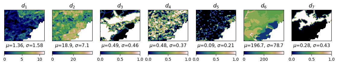
Figure A1 Maps of the seven physical descriptors in the MedEst area at a resolution of 0.01° in the WGS84 projection, where μ and σ represent the spatial average and standard deviation for each descriptor.

Appendix B: Further results and visualizations

Table B1 presents the statistical quantities (mean, median, and standard deviation) of the calibrated hydrological parameters across the 235 French catchments, obtained using different methods.

Figures B1–B3 present similar graphs to Figs. 8, 9, and 11, but these are obtained using local calibrations of spatially distributed parameters with the hybrid model structure (GRNN.D).

Table B1 Median (mean; standard deviation) of the calibrated hydrological parameters across the study area of 235 catchments.

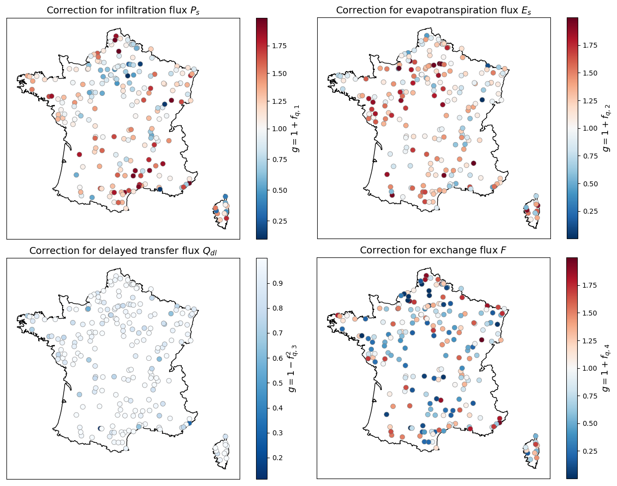
Figure B1 Maps of the spatiotemporal average flux corrections ${\stackrel{\mathrm{‾}}{{\stackrel{\mathrm{‾}}{g\left({\mathit{f}}_q\right)}}^{x\in {\mathrm{\Omega }}_j}}}^t$, where j=1…N_g for the N_g=235 catchments, obtained through local calibrations of spatially distributed parameters with the hybrid model structure (GRNN.D). The function g(.) represents the transformation applied to the neural network output f_q, which may differ depending on the specific flux being corrected. Red indicates corrections that tend to increase the current flux, while blue indicates corrections that reduce it, with white representing minimal or no effective correction.

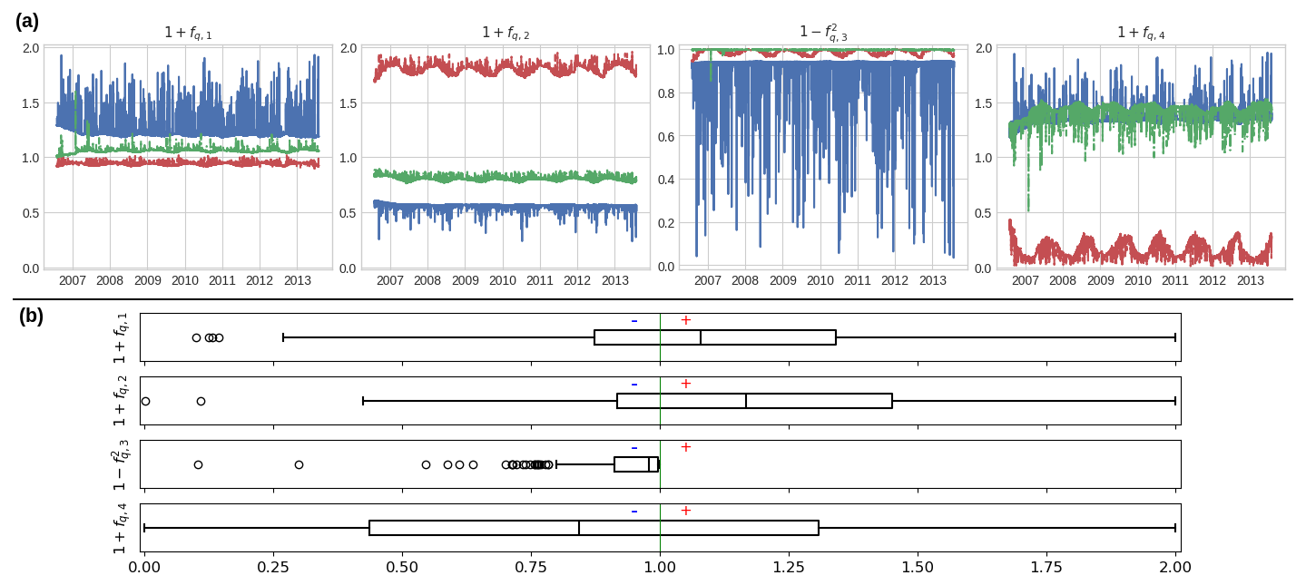
Figure B2 (a) Spatially averaged flux correction time series ${\stackrel{\mathrm{‾}}{g\left({\mathit{f}}_q\left(t\right)\right)}}^{x\in {\mathrm{\Omega }}_j}$ for the same three catchments selected in Fig. 9a. These are obtained through local calibrations of spatially distributed parameters with the hybrid model structure (GRNN.D). (b) Boxplot of the spatiotemporal average flux corrections ${\stackrel{\mathrm{‾}}{{\stackrel{\mathrm{‾}}{g\left({\mathit{f}}_q\right)}}^{x\in {\mathrm{\Omega }}_j}}}^t$, where each boxplot represents 235 catchment-specific spatiotemporal averages.

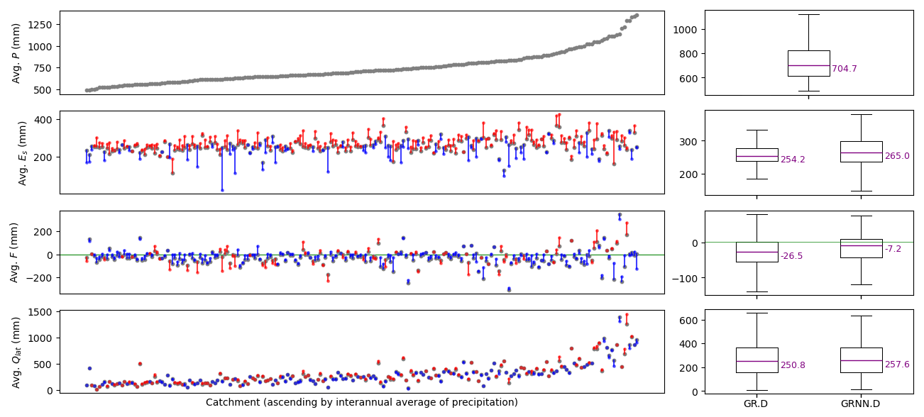
Figure B3 Comparison of mass fluxes affecting the water balance in the interannual mean at the basin scale over the 235-catchment set for the classical GR model (GR.D) and the ϕ₁-hybrid model (GRNN.D), using distributed mapping “D” for conceptual parameters θ in local calibration. The x axis shows 235 catchments, sorted by their average precipitation. Grey dots represent the interannual averages of precipitation P, actual evapotranspiration E_s, exchange flux F, and lateral discharge Q_lat over the calibration period for the classical model. Red dots and lines represent increases according to the hybrid model, while blue ones indicate decreases. For cases where F<0, red indicates a larger magnitude in F for the hybrid model (more negative), while blue indicates a lower magnitude (closer to 0).

Figure B4 presents similar results to Fig. 9a but is plotted using a heatmap over all 235 catchments for both GRNN.U and GRNN.D.

Figure B5 shows graphs similar to those in Fig. 7a but presents different evaluation metrics, including mean absolute error (MAE), percent bias (PBIAS), and peak flow ratio (PFR).

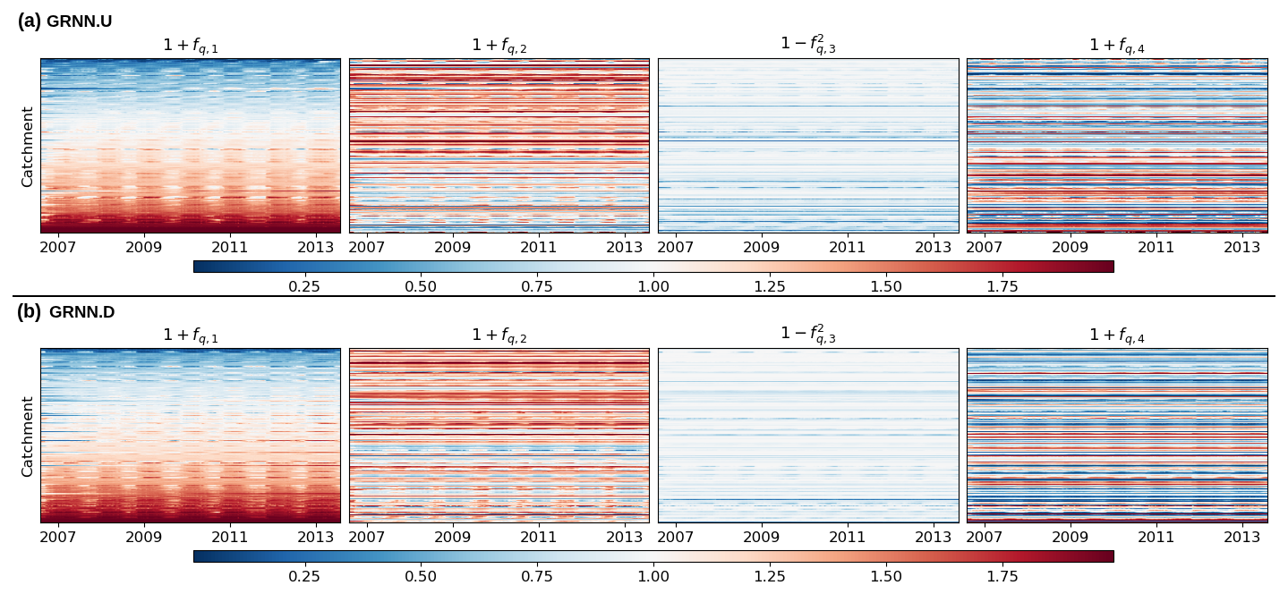
Figure B4 Heatmap of spatially averaged flux correction time series ${\stackrel{\mathrm{‾}}{g\left({\mathit{f}}_q\left(t\right)\right)}}^{x\in {\mathrm{\Omega }}_j}$, where j=1…N_g for the N_g=235 catchments. These are obtained through local calibrations of (a) spatially uniform parameters with the hybrid model structure (GRNN.U) and (b) spatially distributed parameters with the hybrid model structure (GRNN.D).

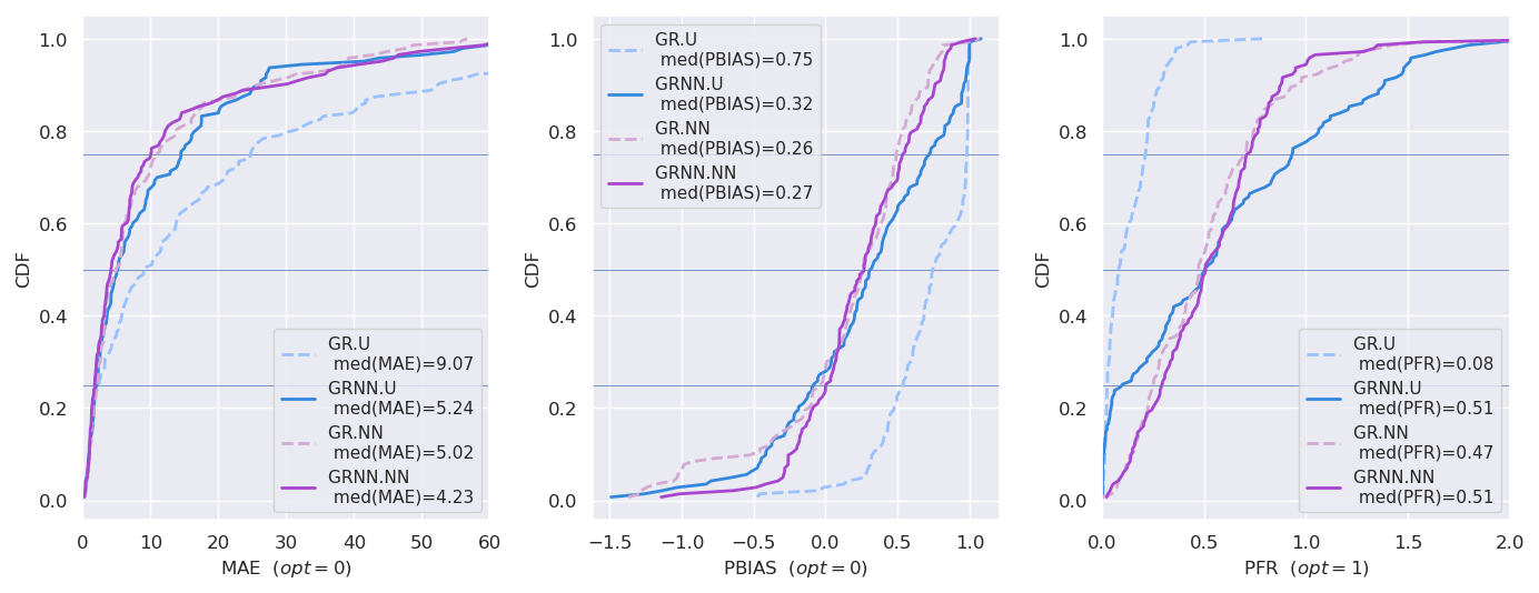
Figure B5 Comparison of mean absolute error (MAE), percent bias (PBIAS), and peak flow ratio (PFR) metrics computed for 143 flood events detected in the validation period across 21 catchments in the MedEst region.

Figure B6 presents graphs similar to those in Fig. 10, but these are obtained using the fully integrated hybrid model, which includes both the process-parameterization neural network and the regionalization neural network (GRNN.NN).

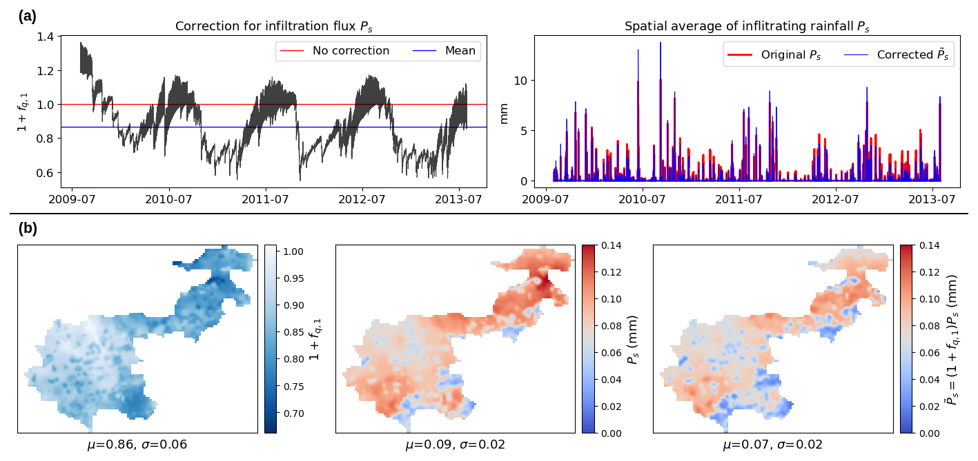
Figure B6 Visualization of flux corrections in the MedEst region obtained through regional calibration of spatially distributed parameters with the fully integrated hybrid model (GRNN.NN). (a) Spatial average of the infiltrating flux correction ${\stackrel{\mathrm{‾}}{\mathrm{1}+f_{q,\mathrm{1}}\left(t\right)}}^x$ and the original and corrected infiltrating rainfall ${\stackrel{\mathrm{‾}}{P_s\left(t\right)}}^x$ and ${\stackrel{\mathrm{‾}}{{\stackrel{\mathrm{̃}}{P}}_s\left(t\right)}}^x$. (b) Maps of the time-averaged infiltrating flux correction ${\stackrel{\mathrm{‾}}{\mathrm{1}+f_{q,\mathrm{1}}\left(x\right)}}^t$ and the original and corrected infiltrating rainfall ${\stackrel{\mathrm{‾}}{P_s\left(x\right)}}^t$ and ${\stackrel{\mathrm{‾}}{{\stackrel{\mathrm{̃}}{P}}_s\left(x\right)}}^t$, where μ and σ represent the spatial average and standard deviation.