State updating of the Xin'anjiang model: joint assimilating streamflow and multi-source soil moisture data via the asynchronous ensemble Kalman filter with enhanced error models

Assimilating either soil moisture or streamflow individually has been well demonstrated to enhance the simulation performance of hydrological models. However, the runoff routing process may introduce a lag between soil moisture and outlet discharge, presenting challenges in simultaneously assimilating the two types of observations into a hydrological model. The asynchronous ensemble Kalman filter (AEnKF), an adaptation of the ensemble Kalman filter (EnKF), is capable of utilizing observations from both the assimilation moment and the preceding periods, thus holding potential to address this challenge. Our study first merges soil moisture data collected from field soil moisture monitoring sites with China Meteorological Administration Land Data Assimilation System (CLDAS) soil moisture data. We then employ the AEnKF, equipped with improved error models, to assimilate both the observed outlet discharge and the merged soil moisture data into the Xin'anjiang model. This process updates the state variables of the model, aiming to enhance real-time flood forecasting performance. Tests involving both synthetic and real-world cases demonstrates that assimilation of these two types of observations simultaneously substantially reduces the accumulation of past errors in the initial conditions at the start of the forecast, thereby aiding in elevating the accuracy of flood forecasting. Moreover, the AEnKF with the enhanced error model consistently yields greater forecasting accuracy across various lead times compared to the standard EnKF.

1 Introduction

Floods, as one of the most frequent natural disasters, significantly affect infrastructure and agricultural yields and may even directly endanger the lives of local residents (Johnson et al., 2020). The destructiveness of flash floods is particularly notable. In recent decades, flash floods triggered by localized torrential rains have frequently resulted in significant human casualties (Pilon, 2002). Short-term flood forecasting, a vital non-structural approach to flood mitigation, plays a crucial role in facilitating emergency responses in flood-prone regions (Craninx et al., 2021). Hydrological models are instrumental in flood forecasting, utilizing mathematical and physical representations to analyze the various components of the catchment hydrological processes, including precipitation, evaporation, and runoff, as well as their interplay. This understanding aids in comprehending catchment hydrological characteristics and trends, which is crucial for simulating and forecasting hydrological processes. The Xin'anjiang model, extensively applied in operational short-term flood forecasting in China, stands as one of the well-known semi-distributed hydrological models. Its broad applicability, especially in the humid and semi-humid climate zones of the Yangtze River basin, has been substantiated by extensive studies (e.g., Fang et al., 2017; Gong et al., 2021; Zang et al., 2021).

However, in hydrological simulations, multiple sources of uncertainty, such as uncertainties in model inputs, structure, and parameters, can significantly affect the accuracy of the simulations (Beven, 1993; Ajami et al., 2007). In short-term flood forecasting, an additional process, often referred to as the real-time correction process, is typically employed to mitigate these uncertainties. A notable strategy in real-time correction involves the recursive adjustment of the hydrological model's state variables based on available real-time observational data. It helps reduce the error accumulation in the initial conditions of hydrological model, a factor that has been identified as a primary source of uncertainty at the start of flood forecasting (Shukla and Lettenmaier, 2011; Yossef et al., 2013; Thiboult et al., 2016). This process is sometimes termed hydrological data assimilation in literature (e.g., Clark et al., 2008). The ensemble Kalman filter (EnKF) (Evensen, 2003), which includes ensemble forecasting concepts with the Kalman filter and employs Monte Carlo methods for error statistical prediction, effectively addresses the inability of Kalman filtering to handle non-linear systems. Its robustness, flexibility, and ease of use have led to its widespread application in hydrological data assimilation (Clark et al., 2008; Liu et al., 2012; Rakovec et al., 2012; Piazzi et al., 2021).

Data assimilation typically falls into two categories: synchronous and asynchronous methods. Synchronous methods depend solely on observational data at a specific update moment, while asynchronous methods broaden this scope by incorporating data over a time frame, including both current and preceding time steps (Sakov and Bocquet, 2018). This distinction is particularly crucial in sequential assimilation, where commonly employed sequential filters like the EnKF utilize a synchronous strategy. Conversely, the asynchronous strategy is predominantly used in smoothers, such as the ensemble Kalman smoother (EnKS) (Evensen and van Leeuwen, 2000). While the EnKS augments reanalysis by integrating future observational data backwards in time, its forecasting efficacy (including real-time forecasting) aligns with that of the EnKF (Evensen, 2009). The intrinsic difference between smoothers and filters is their focus: smoothers assimilate future observational data, while filters process past observational data (Rakovec et al., 2015). Hence, in hydrological data assimilation with a focus on forecasting, filters are generally the preferred choice over smoothers.

In recent years, researchers have made strides in integrating asynchronous strategies into filters for sequential assimilation. This is notably evident in the development of the four-dimensional ensemble Kalman filter (4D-EnKF) (Hunt et al., 2004) and the four-dimensional local ensemble transform Kalman filter (4D-LETKF) (Hunt et al., 2007). The 4D-EnKF stands out for its ability to synchronize the timing of observations with lower computational demands, which is particularly effective in linear dynamics. In contrast, the 4D-LETKF builds upon the 4D-EnKF by prioritizing spatial localization and refining the handling of non-linear observation operators. This enhancement renders it more effective and versatile in managing high-dimensional, chaotic systems, especially in meteorology and climatology. Building on this, Sakov et al. (2010) and Sakov and Bocquet (2018) introduced the asynchronous ensemble Kalman filter (AEnKF). Remarkably, the AEnKF and the 4D-LETKF are essentially equivalent (Sakov et al., 2010), both employing ensemble-based methods to update model states based on observational data. The 4D-LETKF processes asynchronous observations by amalgamating them and updating the state via ensemble transform matrices. Conversely, the AEnKF accomplishes this by advancing corrections along the forecast system trajectory, utilizing ensemble observations from the observation time, thereby efficiently assimilating both past and future data. The AEnKF is designed to be computationally efficient, which is noted for its relative simplicity in implementation compared to the 4D-LETKF. It modifies the standard EnKF using ensemble observations from the time of observations, a straightforward change that does not significantly complicate the assimilation process. The AEnKF technique was first applied by Krymskaya (2013) to the problem of history matching in reservoir engineering. The study revealed that the AEnKF outperforms the EnKF in parameter estimation and utilizes the data with similar efficiency. The AEnKF is recognized for its simplicity and high computational efficiency, offering significant potential in short-term flood forecasting applications. Despite its promise, the scope of research in this area is relatively limited. Among the few studies conducted, Mazzoleni et al. (2018) evaluated AEnKF assimilation in simplified flow routing models, highlighting its exceptional performance in both lumped and distributed flow routing. Tao et al. (2016) summarized the hydrological forecasting test conducted during the 2014 Intense Observing Period of the Integrated Precipitation and Hydrology Experiment (IPHEx-IOP) campaign, proposing a framework for improving flood prediction in mountainous regions through the assimilation of discharge data using the AEnKF method, with a focus on enhancing forecast accuracy and reducing uncertainty. In addition, Rakovec et al. (2015) and our earlier study (Gong et al., 2024) applied the AEnKF to the distributed HBV-96 model and the Xin'anjiang model, respectively. These studies examined the effectiveness of the AEnKF in real-time correction through the assimilation of observed discharge in distributed and semi-distributed hydrological models, revealing that the AEnKF outperforms the standard EnKF. However, these studies assimilate only a single type of observational data (e.g., observed discharge) using the AEnKF method, which does not take full advantage of the AEnKF.

In the context of real-time correction processes employing the AEnKF, the types of observations we assimilate constitute another key factor influencing the effectiveness. Popular observation types that are currently assimilated include discharge, soil moisture, and snow data (Gong et al., 2023). In rainfall–runoff modeling, soil moisture plays a pivotal role in driving the runoff generation process (Massari et al., 2014). A wealth of research has demonstrated that updating hydrological model states through the assimilation of soil moisture significantly enhances the precision of runoff simulations and forecasts (e.g., Wanders et al., 2014; Alvarez-Garreton et al., 2015; Chao et al., 2022). These studies typically rely on a single type of soil moisture dataset. One of the highlights of our study is that it simultaneously considers the advantages of site observation data and soil reanalysis datasets, enhancing both the timeliness and the spatial accuracy of the soil moisture data. Specifically, in the real-time correction process of flood forecasting, there is a high demand for the timeliness of observational data to swiftly respond to flood events. Satellite remote sensing data and reanalysis products often suffer from delays in data release or lengthy observational intervals. In contrast, ground-based soil moisture measurements offer high accuracy and timeliness but are limited to point-scale data, failing to capture the spatial distribution of soil moisture. To overcome this limitation, the weighted k-nearest-neighbor (WKNN) algorithm (Pedregosa et al., 2011; Jung and Lee, 2017) is employed to fuse ground soil moisture measurements with reanalysis soil moisture data. This approach involves establishing a regression relationship between historical ground and reanalysis data, subsequently generating real-time, spatially distributed fusion soil moisture data from current ground observations. On the other hand, discharge observations, due to their direct relevance to flow or water level predictions crucial in flood forecasting, are another valuable choice for assimilation. They provide a comprehensive view of the hydrological conditions of a catchment. Discharge measurements are often more accessible and offer more timely data than soil moisture readings, generally yielding greater reliability (Li et al., 2013). Numerous studies have concentrated on assimilating observed discharge data to enhance flood forecasting, showcasing the substantial potential and impressive effectiveness of this strategy across various regions (e.g., Clark et al., 2008; Sun et al., 2020; Gong et al., 2023). Given that assimilating soil moisture or discharge alone can provide acceptable results, exploring the simultaneous assimilation of both observation types warrants consideration. Previous studies have highlighted the benefits of concurrently assimilating various observation types. Techniques such as the EnKF (Meng et al., 2017), variational assimilation (VAR) (Lee et al., 2011), and tempered particle filter (TPF) (García-Alén et al., 2023) have consistently shown that joint assimilation generally surpasses the efficiency of single-type assimilation. Although these findings are encouraging, the advantage of joint assimilation may not always hold. This is partly because each observation type represents a specific hydrological process, with correlations among variables varying across different spatial and temporal scales. For instance, soil moisture immediately responds to rainfall, while streamflow responses are inherently delayed due to the time delay in the routing process (Meng et al., 2017). Such delays can lead to the accumulation of uncertainties in discharge predictions, which is an aspect often overlooked in synchronized assimilation methods. Contrarily, the AEnKF method considers all observational data within a specific time window rather than just a single observation at the update time, effectively considering the time delays in routing processes and offering a novel approach for the combined assimilation of diverse observation types. However, to our knowledge, there are no existing studies on the performance of the AEnKF in assimilating multiple types of observational datasets (such as soil moisture and discharge measurements), which could significantly improve the accuracy of short-term flood forecasting.

In AEnKF assimilation, ensemble dispersion is achieved by introducing pre-determined noise (commonly zero-mean Gaussian noise) into model state variables and forcing data. The models governing these perturbations are termed error models, and their associated parameters are known as hyperparameters (Thiboult and Anctil, 2015). Improper handling of these uncertainties can potentially impair the efficacy of ensemble-based Kalman filters (Crow and Van Loon, 2006; Pathiraja et al., 2018). The commonly adopted practice involves setting the hyperparameters of error models based on the empirical knowledge of hydrologists or forecasters (e.g., Weerts and El Serafy, 2006; Clark et al., 2008; Sun et al., 2020). This approach is highly subjective, resulting in forecast results that may significantly differ among practitioners. The maximum a posteriori estimation (MAP) method (Li et al., 2014; Gong et al., 2023) represents a Bayesian inference technique specifically designed for ensemble-based Kalman filters. This method leverages historical observational data to objectively estimate the hyperparameters in error models, thereby substantially mitigating the subjectivity associated with hyperparameter configuration. Notably, the strengths of MAP method, compared to alternatives like the kernel conditional density estimation method (Pathiraja et al., 2018), include its independence from the need for sequential observations to be independent themselves. Furthermore, it enables concurrent estimation of hyperparameters across diverse error models, making it particularly compatible with the error models employed in the AEnKF. Another challenge in AEnKF assimilation is reducing the systematic biases that arise from perturbations. When creating ensemble dispersion using error models, it is implicitly assumed that the introduction of noise will not lead to systematic biases in the model outputs (Ryu et al., 2009). Nevertheless, the strong non-linearity of hydrological models and the stringent physical limitations on some state variables mean that even zero-mean Gaussian perturbations may result in systematic biases (Alvarez-Garreton et al., 2015). A case in point is soil moisture, which must stay below saturation levels. During flooding, when soil moisture approaches saturation, perturbing this variable risks breaching these physical boundaries. Subsequent corrections made by the hydrological model to align with saturation levels may introduce truncation errors in the prediction of the background field. To counter this, our study incorporates the bias-corrected Gaussian error model (BGEM) (Ryu et al., 2009), which introduces an unperturbed model run in parallel with the ensemble. This unperturbed model is utilized to correct the biases induced by perturbations. Our prior research (Gong et al., 2024) has shown that the BGEM is effective in alleviating systematic biases caused by random perturbations in soil moisture state variables. However, the performance of the AEnKF with these enhanced error models when assimilating multiple types of observations has yet to be further tested.

This study developed an efficient joint data assimilation framework for real-time correction of short-term flood forecasting based on the AEnKF with improved error models. One of the main highlights of this study is the consideration of the inherent limitations of single-source soil moisture data. By fusing ground-based soil moisture measurements with reanalysis data from the China Meteorological Administration Land Data Assimilation System (CLDAS), the study generates a reliable, real-time spatial distribution dataset of soil moisture that aligns with the 8 h observation intervals of monitoring sites. The second highlight is that the AEnKF with improved error models fully accounts for the time delays in routing process, enabling effective joint assimilation of soil moisture data and discharge observations. Upon establishing the appropriate assimilation time window for the AEnKF with improved error models, the study conducted a detailed comparison between the joint assimilation scheme and individual assimilation schemes (including the separate assimilation of soil moisture or discharge observation data) using synthetic and real-world cases. This comparison effectively underscores the superior performance of the joint assimilation framework proposed in this study.

2 Methodology

2.1 Hydrological model

The Xin'anjiang model, conceptualized by Zhao (1992), is a commonly used hydrological model primarily based on a saturation-excess mechanism. Renowned for its straightforward structure and explicit parameter definitions, this model excels in simulating humid catchments, making it a popular tool for flood forecasting in China. To account for spatial variability, the model typically divides a catchment into sub-catchments. These sub-catchments act as computational units for runoff generation and routing.

The Xin'anjiang model demands relatively simple forcing data, and key inputs include the areal mean rainfall depth (P) and pan evaporation (EM) for each sub-catchment. The model typically comprises four main components: evapotranspiration, runoff production, runoff separation, and flow routing, involving the calibration of 16 distinct parameters. The flow chart of the Xin'anjiang model is presented in Fig. 1. Soil evaporation is derived from pan evaporation data using a three-layer soil moisture module. The runoff generation is based on a saturation-excess mechanism, where runoff is produced only when the soil moisture in the unsaturated zone reaches field capacity. The lag-and-route method calculates the outflow from each sub-catchment. Flow routing from the sub-catchment outlets to the total catchment outlet employs the Muskingum method to successive sub-reaches. It is implemented by dividing the channel from each sub-catchment outlet to the total catchment outlet into varying numbers of sub-reaches. These sub-reaches are based on the distance from each sub-catchment outlet to the total catchment outlet. In addition, the catchment inflow to the outlet is directly calculated by the Muskingum method.

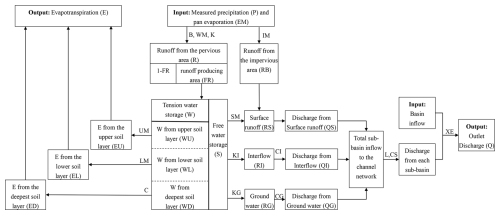
Figure 1 Flow chart of the Xin'anjiang model. The variables in the boxes indicate the model state, inputs, and outputs, and the symbols outside the corresponding blocks are model parameters.

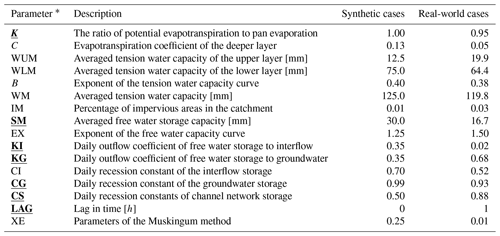
Zhao (1992) categorized the parameters of the Xin'anjiang model into sensitive and non-sensitive groups. In real-world cases, non-sensitive parameters are assigned values based on expert judgment, while optimal values for sensitive parameters are derived from historical data using the shuffled complex evolution (SCE-UA) method (Duan et al., 1992). For synthetic cases, however, parameters are taken to have recommended default values. Table 1 summarizes these parameters.

Table 1 Parameters of the Xin'anjiang model.

^* Bold and underlined parameters indicate that they are sensitive parameters.

2.2 Asynchronous ensemble Kalman filter

The asynchronous ensemble Kalman filter (AEnKF) represents a straightforward enhancement of the ensemble Kalman filter (EnKF), utilizing the same assimilation framework as the EnKF. We follow the notation of Ide et al. (1997) and Vetra-Carvalho et al. (2018) as closely as possible, aiming to make our paper accessible and practical for both data assimilation specialists and a broader audience interested in applying these methods. To this end, the dimensions of the state space and observation space, denoted as N_x and N_y. Further, the time index is always denoted in parentheses to the right of the variable, i.e., (.)(t_i). Notably, the observational data are categorized into two types: the observed discharge at the catchment outlet and soil moisture across sub-catchments. During an ensemble run of the dynamic model, the assimilation process has two steps: the soil moisture observations are used to update the soil states, and the discharge observations are used to update the cumulative channel flow. Consequently, for each assimilation process, the values of N_y can differ, and the same applies to N_x.

2.2.1 Ensemble Kalman filter

At a given time t_i, we define the model state vector as $\mathit{x}\left(t_i\right)\in {\mathcal{R}}^{N_x}$ and the observation vector as $\mathit{y}\left(t_i\right)\in {\mathcal{R}}^{N_y}$. In the EnKF framework, it is crucial to generate a set of independent model state vectors. These vectors constitute an ensemble matrix, denoted as $\mathbf{X}\left(t_i\right)\in {\mathcal{R}}^{N_x\times N_{\mathrm{e}}}$, where N_e is the total number of the ensemble members. The initial X(0) is obtained by the Monte Carlo method.

The state transfer equation at the forecast step is represented by

$$\begin{array}{}\text{(1)}& {\mathit{x}}_j^f\left(t_{i+\mathrm{1}}\right)=\mathcal{M}\left[{\mathit{x}}_j^a\right(t_i),\mathbf{U}(t_i\left)\right]+\mathit{\eta }\left(t_i\right),\end{array}$$

where $\mathcal{M}[.]:{\mathcal{R}}^{N_x}\to {\mathcal{R}}^{N_x}$ signifies the dynamic model, such as the Xin'anjiang model; U(t_i) represents the forcing data (including rainfall and evaporation); and $\mathit{\eta }\left(t_i\right)\in {\mathcal{R}}^{N_x}$ symbolizes the process or system noise characterized by a mean of zero and covariance matrix Q(t_i). In addition, the subscript j signifies the ensemble index, ranging from 1 to N_e. The forecasted values from the dynamic model are marked with a superscript f, while the analysis (updated) values from the filter are denoted by a superscript a.

During the analysis step, we create a set of new observation vectors by perturbing the original observation vector y(t_i), as described by

$$\begin{array}{}\text{(2)}& {\mathit{y}}_j^o\left(t_i\right)=\mathit{y}\left(t_i\right)+\mathit{\epsilon }\left(t_i\right),\end{array}$$

where ${\mathit{y}}_j^o\left(t_i\right)\in {\mathcal{R}}^{N_y}$ represents the perturbed observation vector for the jth ensemble and $\mathit{\epsilon }\left(t_i\right)\in {\mathcal{R}}^{N_y}$ is Gaussian noise characterized by covariance matrix R(t_i). We assume spatial independence of observation errors, thereby designating R(t_i) as a diagonal matrix. Furthermore, the state update equation is expressed as follows:

$$\begin{array}{}\text{(3)}& {\mathit{x}}_j^a\left(t_i\right)={\mathit{x}}_j^f\left(t_i\right)+\mathbf{K}\left(t_i\right)\cdot \left({\mathit{y}}_j^o\right(t_i)-\mathcal{H}[{\mathit{x}}_j^f\left(t_i\right)\left]\right),\end{array}$$

where ℋ[.] is the measurement operator that maps the state space to the observation space, which is also the Xin'anjiang model in this study, and K(t_i) is the Kalman gain matrix calculated by

$$\begin{array}{}\text{(4)}& \mathbf{K}\left(t_i\right)={\mathbf{P}}^f\left(t_i\right){\mathbf{H}}^T\left[{\mathbf{HP}}^f\right(t_i){\mathbf{H}}^T+\mathbf{R}(t_i){]}^{-\mathrm{1}}.\end{array}$$

In scenarios where the state space dimensionality, N_x, is substantial, bypassing the direct computation of P^f(t_i) in favor of calculating P^f(t_i)H^T and HP^f(t_i)H^T emerges as a strategy to enhance computational efficiency, as highlighted by Nerger and Hiller (2013).

2.2.2 Asynchronous variant

The AEnKF is based on the concept of joint state–observation space, where the ensemble is replaced by a joint ensemble that combines state and observation information. Updating model states involves considering observations from both current and previous time steps, controlled by the assimilation time window, tw. This window defines the duration over which observations are considered for the analysis, for instance, including data from the previous 5 h. Moreover, when assimilating only current observations (tw=0), the AEnKF reverts to the standard EnKF. In the AEnKF, the observation vector is altered to

$$\begin{array}{}\text{(5)}& \stackrel{\mathrm{̃}}{\mathit{y}}\left(t_i\right)=\left[\mathit{y}\right(t_i{)}^T,\mathit{y}(t_{i-\mathrm{1}}{)}^T,\mathrm{\dots },\mathit{y}\mathbf{(}{t}_{i-\mathrm{tw}}{)}^T{]}^T\in {\mathcal{R}}^{(\mathrm{tw}+\mathrm{1})\cdot N_y},\end{array}$$

where $\stackrel{\mathrm{̃}}{\mathit{y}}\left(t_i\right)$ is the joint observation vector and $\stackrel{\mathrm{̃}}{\mathbf{R}}\left(t_i\right)$ denotes the covariance matrix of the associated observation noise, expressed as a diagonal matrix:

$$\begin{array}{}\text{(6)}& \stackrel{\mathrm{̃}}{\mathbf{R}}\left(t_i\right)=\left[\begin{array}{ccc}\mathbf{R}\left(t_i\right)& \mathrm{\dots }& \mathrm{0}\\ \mathrm{⋮}& \mathbf{R}\left(t_{i-\mathrm{1}}\right)& \mathrm{⋮}\\ & \mathrm{\ddots }& \\ \mathrm{0}& \mathrm{\dots }& \mathbf{R}\left(t_{i-\mathrm{tw}}\right)\end{array}\right].\end{array}$$

Similarly, the model prediction vector from the prior tw time steps in the observation space is used to expand the state vector:

$$\begin{array}{}\text{(7)}& \begin{array}{rl}{\stackrel{\mathrm{̃}}{\mathit{x}}}_j^f\left(t_i\right)& =\left({\mathit{x}}_j^f{\left(t_{i+\mathrm{1}}\right)}^T,\mathcal{H}\left[{\mathit{x}}_j^f\right(t_{i-\mathrm{1}}){]}^T,\mathcal{H}[{\mathit{x}}_j^f\left(t_{i-\mathrm{2}}\right){]}^T,\right.\\ & {\left.\mathrm{\dots },\mathcal{H}\left[{\mathit{x}}_j^f\right(t_{i-\mathrm{tw}}){]}^T\right)}^T\in {\mathcal{R}}^{N_x+\mathrm{tw}\cdot N_y}.\end{array}\end{array}$$

Furthermore, the new state definition introduces an augmented observation operator $\stackrel{\mathrm{̃}}{\mathcal{H}}\left(t_i\right)$:

$$\begin{array}{}\text{(8)}& \stackrel{\mathrm{̃}}{\mathcal{H}}=\left[\begin{array}{ccc}\mathcal{H}& \mathrm{\dots }& \mathrm{0}\\ \mathrm{⋮}& I_i& \mathrm{⋮}\\ & \mathrm{\ddots }& \\ \mathrm{0}& \mathrm{\dots }& I_{i-\mathrm{tw}}\end{array}\right],\end{array}$$

where I, with the corresponding subscript, stands for a series of identity elements on the diagonal, matching the dimensions in Eq. (7).

Following these augmented equations for ${\stackrel{\mathrm{̃}}{\mathit{x}}}_j^f\left(t_i\right)$, $\stackrel{\mathrm{̃}}{\mathit{y}}\left(t_i\right)$, $\stackrel{\mathrm{̃}}{\mathbf{R}}\left(t_i\right)$, and $\stackrel{\mathrm{̃}}{\mathcal{H}}$, we can directly apply these augmented variables in the EnKF process (Sect. 2.2.1) to implement AEnKF assimilation. Crucially, in the joint state vector ${\stackrel{\mathrm{̃}}{\mathit{x}}}_j^f\left(t_i\right)$, model prediction vectors within the observation space, such as $\mathcal{H}\left[{\mathit{x}}_j^f\left(t_{i-\mathrm{1}}\right)\right]$ and others, are considered diagnostic variables instead of state variables. As a result, they are not updated during the analysis step. Specifically, in Eq. (3), only the first N_x elements of the vector ${\stackrel{\mathrm{̃}}{\mathit{x}}}_j\left(t_i\right)$ are calculated, while others are disregarded.

2.3 Error estimation

Both the EnKF and its variant update model states by employing a weighted average of observational data and model forecasts. This process highlights the crucial role of model and observational errors in determining the effectiveness of the assimilation system. In rainfall–runoff modeling in particular, where uncertainties in both model and observations are inherently ambiguous, generalizing these uncertainties is instrumental in acquiring refined approximations of suboptimal model states. A common technique involves adding unbiased noise to observations, model forcing, and model states.

Observations involved in this study include discharge at the catchment outlet and observed soil moisture. We generalize the observational errors as Gaussian perturbations related to the corresponding observed values (Weerts and El Serafy, 2006; Clark et al., 2008; Alvarez-Garreton et al., 2015). Given that rainfall serves as the most critical input information for the hydrological model, we employ log-normal multiplicative perturbations to describe the errors associated with rainfall, thereby representing the uncertainty in model forcing (McMillan et al., 2011; DeChant and Moradkhani, 2012). Moreover, we introduce a first-order autoregressive model to represent the temporal correlation within the observational errors and the forcing errors.

In the assimilation of observed discharge at catchment outlet, the key model state variable updated is cumulative channel flow. This variable represents the outflow from each sub-catchment on the routing calculation unit (sub-reaches in this study), denoted as QC. As Li et al. (2014) conclude, this state variables are perturbed using a Gaussian function. When assimilating observed soil moisture, the model state variables representing soil humidity need to be updated. Specifically, this refers to the tension water storage (including upper- and lower-layer tension water) and the free water storage in the Xin'anjiang model. In the Xin'anjiang model, the soil moisture state variables receive physical constraints. The free water storage (denoted as S) reflects the soil moisture in the topsoil layer, specifically the humus layer (Yao et al., 2012). Therefore, it is assumed that the free water storage can be considered to range between the saturation moisture content and the field capacity, with its upper limit controlled by the parameter SM and the lower limit set to zero. On the other hand, the tension water storage (denoted as W) represents the soil moisture throughout the entire soil profile, encompassing the whole unsaturated zone (Yao et al., 2012). Consequently, the tension water storage is considered to vary between the field capacity and the wilting point, with its upper limit governed by the parameter WM and the lower limit being zero. The WU, WL, and WD represent the upper-, lower-, and deep-layer tension water storage, respectively, with their upper limits controlled by the parameters WUM, WLM, and WDM and $\mathrm{WM}=\mathrm{WUM}+\mathrm{WLM}+\mathrm{WDM}$. When the variables approach the upper or lower limit, the Gaussian perturbations may cause it to violate the physical constraints. If the hydrological model corrects it, it will lead to the truncation error in the background field predictions. We introduce the bias-corrected Gaussian error model (BGEM) proposed by Ryu et al. (2009), which is aimed at reducing biases that emerge due to adherence to physical constraints.

The aforementioned error models are controlled by parameters known as hyperparameters (Thiboult and Anctil, 2015), such as the hyperparameters for Gaussian perturbations, which are the mean and standard deviation. We apply the maximum a posteriori estimation method (MAP) to identify the globally optimal values of these hyperparameters (Gong et al., 2023). The MAP method aims to maximize the probability density of the hyperparameters with given the observed historical flood events. Section S1 in the Supplement provides a comprehensive introduction to the implementation of error estimation in this study.

2.4 Multi-source soil moisture data fusion

The soil moisture reanalysis data are sourced from the China Meteorological Administration Land Data Assimilation System (CLDAS) near-real-time dataset (National Meteorological Information Centre, 2017). While the CLDAS dataset demonstrates a reasonable level of accuracy within China, with a regional average correlation coefficient of 0.89, a root mean squared error of 0.02 m³ m⁻³, and a bias of 0.01 m³ m⁻³ (Wang and Li, 2020), it faces limitations due to missing values in some areas and data latency (published with a 2 d lag), restricting its application in real-time flood forecasting in small and medium-sized catchments. On the other hand, ground station measurements offer high precision and timeliness (real-time data) but represent point-scale soil moisture, while the Xin'anjiang model simulates soil moisture as areal averages for sub-catchments, necessitating the consideration of spatial-scale effects. To bridge this gap and assimilate soil moisture observations into the Xin'anjiang model, this study employs the weighted k-nearest-neighbor (WKNN) algorithm (Pedregosa et al., 2011) to merge CLDAS soil moisture data (hereinafter referred to as CLDAS) with in situ soil moisture data collected from monitoring sites (hereinafter referred to as IN SITU). This method generates real-time, spatially distributed soil moisture data based on in situ observations and the spatial distribution from the CLDAS dataset, ensuring compatibility with the tension water storage and free water storage in the Xin'anjiang model.

The Harmonized World Soil Database (HWSD) provides a soil texture map for two layers: 0–30 cm (topsoil layer, T) and 30–100 cm (subsoil layer, S). Initially, using the technique by Reynolds et al. (2000), soil transfer functions are applied to the grid of the soil texture map. This process involves estimating the wilting point, θ_wp; field capacity, θ_fc; and saturation moisture content, θ_s, for each grid layer based on its soil clay and sand percentage contents along with the United States Department of Agriculture (USDA) soil texture classification. In this study, we assume that the soil moisture constants for each sub-catchment are the arithmetic average of the grid-scale soil moisture constants within the corresponding areas.

In the Xin'anjiang model, tension water capacity (WM), corresponding to available water capacity, is defined as the moisture content between the wilting point and field capacity, thus representing the thickness of the unsaturated zone. Free water capacity (SM) is defined as the moisture content between field capacity and saturation moisture content, relating to the thickness of the humus soil layer. Accordingly, we define a conceptual soil profile in the Xin'anjiang model, where the soil profile of tension water is divided into upper, lower, and deep layers. The capacity of each layer is calculated as

$$\begin{array}{}\text{(9)}& \mathbf{WL}={\displaystyle \frac{\mathbf{WWM}}{\left({\mathit{\theta }}_{\mathrm{fc}}-{\mathit{\theta }}_{\mathrm{wp}}\right)}},\end{array}$$

where WL is the soil profile thickness matrix of tension water, $\mathbf{WL}=(\mathrm{WUL},\mathrm{WLL},\mathrm{WWL})$, representing the thickness of the upper, lower, and entire soil profile of tension water in millimeters, respectively, and $\mathbf{WWM}=(\mathrm{WUM},\mathrm{WLM},\mathrm{WM})$. Similarly, the thickness of the conceptual soil profile of free water is calculated as

$$\begin{array}{}\text{(10)}& \mathrm{SL}={\displaystyle \frac{\mathrm{SM}}{\left({\mathit{\theta }}_{\mathrm{s}}-{\mathit{\theta }}_{\mathrm{fc}}\right)}}.\end{array}$$

Subsequently, linear interpolation is used to adjust the in situ data and CLDAS reanalysis soil moisture data, both at varying depths, to match the thickness of the conceptual soil profile. This step is followed by the calculation of tension and free water storage, derived from the transformed in situ and CLDAS data. The calculation formula is as follows:

$$\begin{array}{}\text{(11a)}& {\displaystyle }\left\{\begin{array}{l}{\mathbf{WOB}}_i=\left(\mathit{\theta }\mathit{\_}{\mathbf{WL}}_i-{\mathit{\theta }}_{\mathrm{wp}}\right)\cdot \mathbf{WL}{}^{\prime },\\ \mathbf{WL}{}^{\prime }=\left(\begin{array}{ccc}\mathrm{WUL}& \mathrm{0}& \mathrm{0}\\ \mathrm{0}& \mathrm{WLL}& \mathrm{0}\\ \mathrm{0}& \mathrm{0}& \mathrm{WWL}\end{array}\right),\end{array}\right.\text{(11b)}& {\displaystyle }{\mathrm{SOB}}_i=\left(\mathit{\theta }\mathit{\_}{\mathrm{SL}}_i-{\mathit{\theta }}_{\mathrm{fc}}\right)\cdot \mathrm{SL},\end{array}$$

where SOB and $\mathbf{WOB}=(\mathrm{WUOB},\mathrm{WLOB},\mathrm{WWOB})$, respectively, represent the free water storage and tension water storage at various layers, derived from observation data. These are referred to as the observed free water storage and observed tension water storage. $\mathit{\theta }\mathit{\_}\mathbf{WL}=(\mathit{\theta }\mathit{\_}\mathrm{WUL},\mathit{\theta }\mathit{\_}\mathrm{WLL},\mathit{\theta }\mathit{\_}\mathrm{WWL})$ and θ_SL indicate the soil moisture contents after linear interpolation to the respective conceptual soil profile thicknesses. ${\mathit{\theta }}_{\mathrm{wp}}=({\mathit{\theta }}_{\mathrm{wp}},{\mathit{\theta }}_{\mathrm{wp}},{\mathit{\theta }}_{\mathrm{wp}}$). The subscript i indicates different datasets – namely, IN SITU or CLDAS.

Finally, using the WKNN method, soil moisture data from the IN SITU dataset is integrated with the CLDAS dataset. The specific implementation steps are as follows:

1. Normalize the observed free water content and observed tension water content from the dataset using the min–max normalization method. Denote the normalized observation vector as PSM:

   $$\begin{array}{}\text{(12)}& \mathit{P}\mathit{S}{\mathit{M}}_i=({\mathbf{WOB}}_i{}^{\prime },{\mathrm{SOB}}_i{}^{\prime }).\end{array}$$

2. The Minkowski distance is used to measure the proximity between the IN SITU data under evaluation and historical samples. A smaller distance indicates a closer match between the evaluated soil moisture content and the historical sample. The distance is calculated as follows:

   $$\begin{array}{}\text{(13)}& d={\left(\sum _{j=\mathrm{1}}^n|{\mathrm{psm}}_{\text{IN SITU,}j}^{\mathrm{RTD}}-{\mathrm{psm}}_{\text{IN SITU,}j}^{\mathrm{HD}}{|}^p\right)}^{\mathrm{1}/p},\end{array}$$

   where psm_{IN SITU,j} represents the jth element of the vector PSM_{IN SITU} and n is the dimension of PSM_{IN SITU}. The superscript RTD stands for the data under evaluation, and HD denotes historical data. The distances between the data under evaluation and each historical sample are ranked in ascending order. The K nearest historical samples are then selected as reference indices based on this principle.

3. The inverse distance weighting method is used to calculate the final observed free water storage and observed tension water storage based on the K nearest historical samples:

   $$\begin{array}{}\text{(14a)}& {\displaystyle }{\mathit{\omega }}_m={\displaystyle \frac{\mathrm{1}}{d_m}}/\sum _{m=\mathrm{1}}^K{\displaystyle \frac{\mathrm{1}}{d_m}},\text{(14b)}& {\displaystyle }\mathit{P}\mathit{S}{\mathit{M}}_{\mathrm{RGC}}=\sum _{m=\mathrm{1}}^K{\mathit{\omega }}_m\mathit{P}\mathit{S}{\mathit{M}}_{\mathrm{CLDAS},m},\end{array}$$

   where PSM_RGC is the normalized merged observational soil moisture vector, ω represents the inverse distance weights, and PSM_CLDAS,m is the normalized CLDAS observation data vector corresponding to the mth sample. The merged observed tension water storage, $\mathit{W}\mathit{O}{\mathit{B}}_{\mathrm{RGC}}=({\mathrm{WUOB}}_{\mathrm{RGC}},{\mathrm{WLOB}}_{\mathrm{RGC}},{\mathrm{WWOB}}_{\mathrm{RGC}},)$ and merged observed free water storage, SOB_RGC, are obtained after denormalization

In this study, the grid search (GS) method (Bergstra and Bengio, 2012; Alibrahim and Ludwig, 2021) is employed to optimize the hyperparameters K and p, accompanied by a three-fold cross-validation. This approach ensures maximum R² and minimum root mean squared error for the test set, balancing model generalizability with accuracy (Sect. S2, Table S1). For the multi-source soil moisture data fusion, 70 % of the historical dataset is used as the training set for model training, while the remaining 30 % serves as the test set to verify model generalization.

2.5 Evaluation metrics

In this study, we use four metrics to assess the assimilation effectiveness, focusing on both optimal single-value and ensemble performances, as suggested by McInerney et al. (2020). The optimal single-value performance, indicating the highest simulation accuracy, is represented by the ensemble mean values of the simulated discharge. The ensemble performance evaluation, in contrast, examines the simulated discharge ensemble through the lens of the ensemble forecasting, covering both the overall performance of ensemble and its reliability.

For quantitatively assessing the optimal single-value performance, we employ the normalized Nash–Sutcliffe efficiency coefficient (NNSE) (Nossent and Bauwens, 2012) and the root mean squared error (RMSE). The continuous ranked probability score (CRPS), introduced by Hersbach (2000), measures the overall performance of the ensemble. The reliability component of CRPS, denoted as RELI, focuses on assessing ensemble reliability. For these metrics, we use the ratios of the AEnKF to open loop (ensemble run without assimilation), represented as R_RMSE, R_CRPS, and R_RELI. Moreover, the event-averaged values of these ratios are denoted as MR_RMSE, MR_CRPS, and MR_RELI. The mean value of NNSE for multiple flood events is denoted as MNNSE. In synthetic cases, “synthetic true” values serve as the benchmark for all evaluation metrics, while observed values are used in real-world cases. Additional information about these metrics can be found in Sect. S3.

3 Study area and data

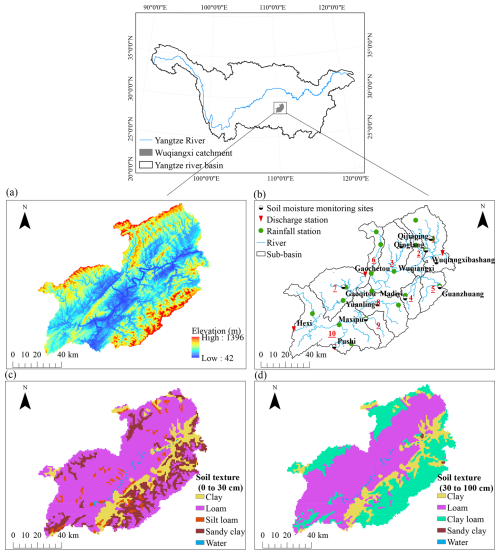
The Wuqiangxi Catchment (Fig. 2), is located in the middle reaches of the Yuan River, the third-largest tributary of the Yangtze River. It covers an area of approximately 8033 km², with elevations ranging from 42 to 1396 m above sea level. The geographical coordinates of the catchment extend from 109°44^′ E to 111°01^′ E and from 28°01^′ N to 29°07^′ N. Situated in the mid-subtropical monsoon humid climate zone, the Wuqiangxi Catchment experiences abundant rainfall and has rich water resources. The average annual precipitation is around 1400 mm, with uneven distribution throughout the year, predominantly during the flood season (March to September). The catchment, located in the subtropical evergreen and deciduous broadleaf forest belt, features dense vegetation, predominantly forests and grasslands. The soil texture is primarily loamy. For this study, the Wuqiangxi Catchment is divided into 10 sub-catchments, each identified by red underlined numbers in Fig. 2b, ensuring at least one rain gauge in each sub-catchment. Among the three discharge stations in the study catchment,Wuqiangxibashang station provides the outflow data at the catchment outlet, while Hexi and Gaochetou are stations that provide inflow data for the study area. Due to the lack of soil moisture and rainfall data within their controlled areas, the control areas of Hexi and Gaochetou are not included in the study. For an overview of the data used in this study, please see Sect. S4.

Figure 2 Study catchment. (a) Digital elevation map (DEM). (b) Sub-catchments and observation stations. (c) Soil texture (0 to 30 cm). (d) Soil texture (30 to 100 cm).

4 Experimental setup

4.1 Warming-up period

In China, hydrometeorological data are typically reported at sub-daily intervals during flood periods and on a daily basis otherwise to support flood forecasting and water resource management. The Xin'anjiang model operates in two modes to meet these needs: it uses hourly simulations for flood forecasting and daily simulations for managing water resources. The hourly simulations require initial soil moisture for each sub-catchment, which is derived from the daily simulations (Chen et al., 2023). Consequently, a daily simulation must be performed prior the hourly simulation, and we recommend that this warming up (spin up) be at least 3 months long. This period enables the soil moisture simulated daily, driven by observed hydrometeorological data, to gradually approaches actual soil moisture (Kim et al., 2018). The influence of initial soil moisture on the daily simulation becomes minimal by the end of the warming-up period, allowing for soil moisture for daily simulation to be used as initial conditions for hourly simulation (Yao et al., 2012). The daily simulation in this study began on 10 February 2014. Testing showed that even in extreme cases where the initial soil moisture in the daily simulation is set to zero or fully saturated, there is almost no impact on the flood simulation results. So, they can be set arbitrarily within reason. In this study, the initial values for the daily simulation are set, with the soil moisture content at half of the saturation value, and the sub-reaches outflow is set to be the observed discharge at the catchment outlet on the start date divided by the total number of sub-reaches.

4.2 Synthetic cases

In the synthetic cases, the hydrological model operates on an hourly time step with a maximum lead time of 24 h, and ensemble simulations involve 100 members. The initial soil moisture is set to half of the maximum value. To ensure consistency in the length of forecast sequences and the comparability of results, the start time for forecasting the same flood event under different lead times is set to the same moment – specifically, the 24 h (maximum lead time) after the flood start time. To capture peak flows even at the maximum lead time, the start of each flood event is advanced by 24 h. However, due to the lack of hourly observations prior to the actual onset of the flood, data for these initial 24 h are derived by interpolating from daily observations. Synthetic data are generated as follows. Firstly, historical flood events are utilized to apply the MAP method, producing an optimal hyperparameter set, $\widehat{\mathit{\psi }}$. Here, ${\widehat{\mathit{\sigma }}}_{\mathrm{lnp}}$ and ${\widehat{\mathit{\alpha }}}_{\mathrm{lnp}}$ control the error model of forcing data (Sect. S1.1). This introduces random perturbations into hourly rainfall observations, creating a set of random rainfall data, referred to as synthetic true rainfall. Similarly, ${\widehat{\mathit{\sigma }}}_{yd}$ and ${\widehat{\mathit{\alpha }}}_{yd}$ manage the observation error model (Sect. S1.2), perturbing catchment inflow to produce a dataset known as synthetic true inflow. Subsequently, the Xin'anjiang model, driven by the synthetic true rainfall and synthetic true inflow, along with the recommended parameters (see Table 1), outputs state variables (such as tension water storage) and discharge at the catchment outlet for each time step. These outputs are designated as the synthetic true state variables and synthetic true discharge. In the final phase, optimal hyperparameter sets $({\widehat{\mathit{\sigma }}}_{ys},{\widehat{\mathit{\alpha }}}_{ys})$ and $({\widehat{\mathit{\sigma }}}_{yd},{\widehat{\mathit{\alpha }}}_{yd})$ are applied to the observation error model. This step introduces random perturbations into the synthetic true state variables and synthetic true discharge, resulting in the creation of synthetic observed state variables and synthetic observed discharge. Specifically, synthetic observations of tension and free water storage are employed to update the simulated values in the Xin'anjiang model. On the other hand, synthetic discharge observation is utilized for updating cumulative channel flow. Both of these assimilation processes are conducted at an hourly interval.

4.3 Real-world cases

In the real-world cases, the time step and number of ensemble members are the same as in the synthetic cases. Similarly to the synthetic cases, to ensure the comparability of results, the forecast start time for all lead times is uniformly delayed from the flood onset (the earliest available hourly data) by a duration corresponding to the maximum lead time. For some flood events, high flow occurred as early as in the ninth hour after onset. To avoid missing the peak flow, the maximum lead time is set to 8 h. The observational tension water storage, WOB_RGC, and free water storage, SOB_RGC, as introduced in Sect. 2.4, are used to assimilate the simulated tension and free water storage in the Xin'anjiang model, with an assimilation interval of 8 h. Additionally, discharge observation is assimilated into the cumulative channel flow with a 1 h interval. Note that in both synthetic and real-world cases in this study, we use historical rainfall data as a perfect proxy for rainfall prediction with the aim of assessing temporal persistence of the assimilation effect without introducing uncertainty from numerical weather prediction. Temporal persistence refers to the duration over which the updating applied to state variables by the AEnKF at the start of forecasting continue to hold in the future.

By introducing the unbiased perturbations into the model forcing and states, and running the Xin'anjiang model in ensemble mode without assimilation, the operation is referred to as open loop (OL). In contrast, an ensemble run integrated with AEnKF assimilation is referred to as the AEnKF. To reduce the effects of random perturbations on outcomes, each flood event in our study is subjected to five repeated ensemble simulations. We then select the simulation corresponding to the median RMSE in the forecasted discharge as our final outcome.

5 Results

5.1 Synthetic cases

5.1.1 Hyperparameter estimation for error models

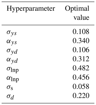
Most current assimilation methods, while suboptimal for complex hydrological processes, still yield reliable outcomes within a reasonably characterized uncertainty. Our approach to error characterization, widely adopted in hydrology, involves perturbing model forcing, observations, and states from an assumed distribution. We applied the MAP method for global hyperparameter optimization, with optimal parameters detailed in Table 2. These optimized hyperparameters are used in error models for both synthetic and real-world cases. However, given the limited number of flood events used for calibration, the hyperparameter optimization, akin to model parameter calibration, might exhibit uncertainty and parameter equifinality, leading to multiple hyperparameter combinations that may produce similar ensemble simulations.

Table 2 Hyperparameters estimated by the MAP method.

5.1.2 The time window of the AEnKF

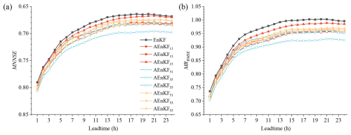
The AEnKF employs observational data from both the current and the preceding time periods for assimilation, with the duration of the past interval defined by the time window, ω. Determining the optimal duration for assimilating past observations is critical for the effectiveness of the AEnKF. If the time window is set too narrowly, the system might fail to fully capitalize on historical data to enhance assimilation precision. On the other hand, an excessively broad time window could lead the non-linear system incorporating irrelevant information from distant past periods, potentially undermining assimilation performance. Therefore, we conducted tests to assess the impact of varying time windows on discharge forecast accuracy. Specifically, for soil moisture observations, we explored three different time windows: ω_s=1 h, ω_s=3 h, and ω_s=5 h. Similarly, for discharge observations, we examined time window, ω_d, values of 1, 3, and 5 h. To facilitate clarity, these assimilation time windows are denoted using dual numerical subscripts. For instance, the AEnKF utilizing ω_s=1 h and ω_d=3 h is designated as AEnKF₁₃, and similar nomenclature applies to other configurations.

The disparity in forecast discharge accuracy across different time windows is presented in Fig. 3. It shows the MNNSE and MR_RMSE metrics for forecast discharge across lead times of 1 to 24 h under assorted time window combinations. It is observed that the performance of the AEnKF varies across these time windows. The most effective assimilation across all lead times is achieved with ω_s=3 h and ω_d=3 h. It is important to note, however, that even with the least effective time windows (ω_s=1 h and ω_d=5 h), performance of the AEnKF still surpasses that of the EnKF. In more detail, the time windows for soil moisture and discharge have complex interactions that collectively influence the forecast results for catchment outlet discharge. For soil moisture assimilation, a 3 h window demonstrates the most significant benefits. In terms of NNSE, the 5 h window outperforms the 1 h in most cases, except when ω_d=3 h, where the reverse is true. In the assimilation of outlet discharge, the 3 h window generally proves most effective but with a larger soil moisture window (ω_s=5 h), as assimilating discharge data with 1 h window yields the best results. Almost universally, the 1 h window performs as well as or surpasses the 5 h window. This indicates that longer assimilation windows do not necessarily yield better results. Therefore, for upcoming studies involving synthetic data cases, the AEnKF will utilize assimilation time windows of ω_s=3 h and ω_d=3 h.

Figure 3 The forecasted discharge accuracy for various time windows for (a) MNNSE and (b) MR_RMSE.

5.1.3 Multivariate observation assimilation scheme

Upon determining the assimilation time window, we meticulously analyzed the variances between three unique AEnKF assimilation strategies. These include the assimilation of solely observed soil moisture (labeled as AEnKF_S), the assimilation of solely observed outlet discharge (labeled as AEnKF_Q), and a joint assimilation of both observations types (labeled as AEnKF_SQ).

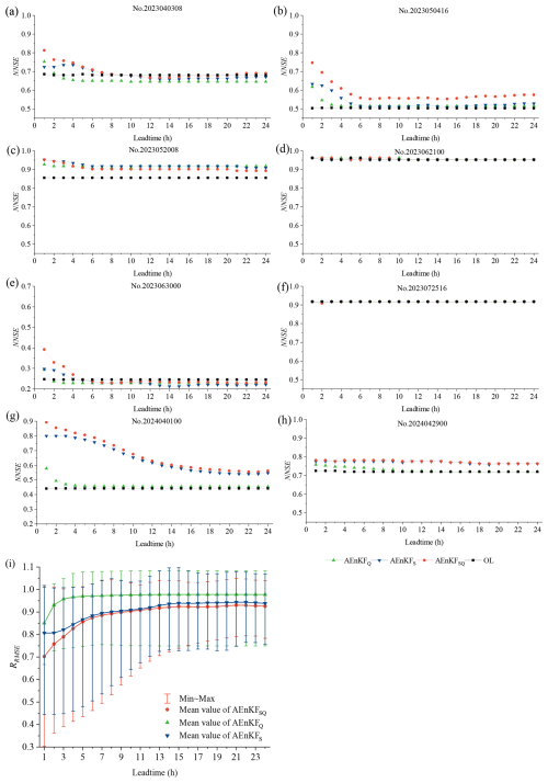
In our assessment of one-step (1 h) prediction of outlet discharge, we examined the optimal single-value performance and ensemble efficacy of the three schemes. The evaluation of the optimal single-value performance was conducted using NNSE and R_RMSE as metrics. Figure 4a–h illustrate the NNSE values during eight flood events in 2023 and 2024 (refer to Table S3). Significantly, in events no. 2023062100 and no. 2023072516, the catchment experienced minimal rainfall (only 1 h of rainfall exceeded 3 mm), with the flood dynamics largely driven by catchment inflows. Consequently, updates to soil moisture within the catchment had no influence on flood progression, and while assimilating observed discharge data slightly enhanced flood forecasting accuracy, the improvement was minimal and could be considered negligible. Conversely, in the other six events where rainfall predominantly influenced the flood dynamics, all three assimilation schemes outperformed the OL mode in NNSE scores, indicating improvements in one-step prediction accuracy to varying extents. Among these, AEnKF_SQ, simultaneously assimilating observed soil moisture and discharge data, notably surpassed the other two schemes. This superiority is further supported by the R_RMSE statistics in Fig. 4i, where the MR_RMSE for AEnKF_SQ showed a decrease of 0.11 and 0.16 compared to AEnKF_S and AEnKF_Q, respectively. Moreover, soil moisture assimilation and discharge assimilation exhibited comparable performances, with only a marginal difference of 0.05 in MR_RMSE.

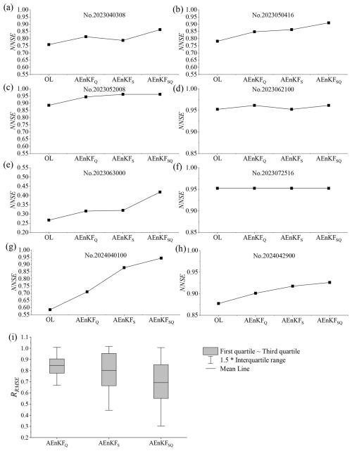
Figure 4 The optimal single-value performance of three AEnKF assimilation schemes for synthetic cases: (a–h) NNSE and (i) R_RMSE.

Subsequently, we conducted an evaluation of the ensemble performance across eight flood events, specifically examining the overall ensemble performance as measured by CRPS and the ensemble reliability as indicated by the RELI metric. In Fig. 5a, the distribution of R_CRPS values is showcased. For the AEnKF_Q scheme, R_CRPS values fluctuated between 0.8 and 1.0, averaging 0.89; for AEnKF_S, the range is from 0.39 to 1.03 with an average of 0.84; and for AEnKF_SQ, it varied from 0.29 to 1.01, averaging 0.74. This demonstrates an enhancement in the overall ensemble performance for all schemes over the OL model, particularly for AEnKF_SQ, which significantly outshone AEnKF_S and AEnKF_Q. Further, AEnKF_S slightly outperforms AEnKF_Q. Figure 5b illustrates the R_RELI scores, showing a similar trend of improved ensemble reliability for all three schemes over OL. Here, the reliability of AEnKF_SQ is notably higher than that of both AEnKF_S and AEnKF_Q. On the other hand, AEnKF_S is more reliable compared to AEnKF_Q.

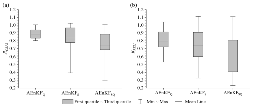
Figure 5 The ensemble performance of three AEnKF assimilation schemes for synthetic cases: (a) R_CRPS and (b) R_RELI.

Within the context of one-step prediction, Fig. 6 presents the R_RMSE for updated state variables of the Xin'anjiang model under three distinct assimilation schemes, involving free water storage; tension water storage across upper, lower, and total layers; and cumulative channel flow across all sub-catchments. As anticipated, in the AEnKF_Q scheme, which solely updates the cumulative channel flow without involving the runoff generation process, the state variables indicative of soil moisture (S, W, WU, WL) remain unaffected. This is reflected in Fig. 6a–d, where the mean R_RMSE values associated with the grey boxes hover around 1.0. In the context of cumulative channel flow, AEnKF_Q generally achieves a reduction in RMSE relative to OL.

In the case of AEnKF_S, updating the soil moisture impacts both runoff generation and subsequent flow routing processes, leading to a response in all state variables. Significantly, the AEnKF_S scheme demonstrates the most substantial corrections in free water storage (S), consistently yielding lower RMSE values than the OL scheme in all instances. When updating the total tension water storage (W), AEnKF_S usually attains lower RMSE values compared to OL. However, this effect is less marked than that for free water storage. This is illustrated in Fig. 6b, where, except for Event 6 and Event 8, the average values associated with the red boxes exceed those in Fig. 6a. Contrastingly, updates to the upper and lower layers of tension water storage in the AEnKF_S scheme produced opposite outcomes, with the RMSE values for these post-update state variables exceeding those of OL. This phenomenon can be attributed to the following: firstly, the initial soil moisture values in this study were set at half of their maximum, and during flood periods, the saturation-excess runoff generation mechanism ensures rapid saturation of both the upper and the lower tension water, reaching the maximum limits (WUM and WLM). Thereafter, due to the physical upper bounds of these variables, the assimilation process is hindered in effectively updating WU and WL values. Consequently, this may lead to a systematic underestimation of these values compared to actual measurements and consequently higher RMSE values than OL. In contrast, free water storage, even during flood periods, may not persistently reach its maximum (SM), resulting in the most advantageous update effect for it. These results highlight the criticality of choosing appropriate state variables for updates in hydrological model state updating, particularly when utilizing methods such as AEnKF.

In the case of AEnKF_SQ, the updates to soil moisture state variables show similarities to those in AEnKF_S. However, when it comes to the updates of cumulative channel flow, AEnKF_SQ effectively integrates the strengths of both AEnKF_Q and AEnKF_S, resulting in a more outstanding performance. This outcome suggests that the concurrent assimilation of both soil moisture and discharge observations can efficiently utilize the advantages of each, leading to a greater assimilation accuracy than the assimilation of a single observation source.

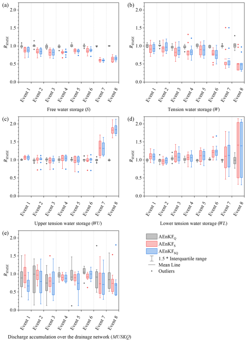
Figure 6 Effects of three assimilation schemes on state variables. (a) Free water storage (S), (b) tension water storage (W), (c) upper tension water storage (WU), (d) lower tension water storage (WL), and (e) cumulative channel flow (QC).

In our assessment, we analyzed the discharge simulation precision of three assimilation schemes over lead times ranging from 1 to 24 h, aiming to gauge the temporal persistence of the assimilation effect. Figure 7a–h present the NNSE for eight flood events. The events identified as no. 2023062100 (Fig. 7d) and no. 2023072516 (Fig. 7f) were mainly driven by inflows, exhibiting only slight improvements in state updates, and therefore are not included in further discussions. For the events identified as no. 2023050416, no. 2023052008, no. 2024040100, and no. 2024042900, the NNSE of each assimilation scheme exceeded that of OL across all lead times, indicating a consistent assimilation impact lasting up to 24 h. For the event labeled no. 2023040308, the temporal persistence for the AEnKF_SQ, AEnKF_S, and AEnKF_Q schemes are noted as 8, 8, and 2 h, respectively; in the case of the event marked as no. 2023063000, these durations are 5, 4, and 1 h. Importantly, it is noteworthy that even in no. 2023063000, despite being the least effective, the NNSE discrepancy between AEnKF_SQ and OL for lead times exceeding 8 h remains below 0.02. Furthermore, AEnKF_SQ demonstrated superior performance in most flood events across all lead times compared to both AEnKF_S and AEnKF_Q. The notable exception is event no. 2023052008, where AEnKF_SQ excelled within a 4 h lead time but slightly lagged behind the other two schemes beyond this duration. Nevertheless, the variance in NNSE for AEnKF_SQ during this event stayed below 0.02. Figure 7i statistically illustrates the R_RMSE values. Notably, the MR_RMSE for each of the three assimilation schemes remains below 1.0 for all lead times, signifying that in terms of event averages, each scheme achieves a temporal persistence of up to 24 h. Additionally, the discharge forecast accuracy across nearly all lead times is ranked with AEnKF_SQ surpassing AEnKF_S, which itself exceeds AEnKF_Q.

Figure 7 Assessment of forecast discharge accuracy across three assimilation schemes during 1 to 24 h lead times for (a–h) NNSE and (i) R_RMSE.

5.2 Real-world cases

In real-world cases, the sensitive parameters of Xin'anjiang model are calibrated based on historical flood events. After global optimization using the SCE-UA, the Xin'anjiang model, equipped with optimally sensitive parameters, exhibited an average NNSE of 0.89 for the calibration events and 0.8 for the validation events, demonstrating reliable and credible flood simulation and forecasting capabilities.

Considering that soil moisture observations are obtained every 8 h in real-world cases as opposed to every 1 h in synthetic cases, we have drawn on synthetic case results to establish an assimilation time window for soil moisture as close as possible to 3 h, set to 8 h. Therefore, ω_s is designated to be 8 h, utilizing only the observations from the current time and those from 8 h earlier for assimilation. For the discharge assimilation, we set the time window to be consistent with the synthetic cases, i.e., ω_d=3 h. Additionally, guided by the insights from synthetic cases, in real-world cases, we incorporate all available soil moisture observations but limit updates to the free water storage component of the Xin'anjiang model.

5.2.1 Fusion of in situ data with CLDAS soil moisture data

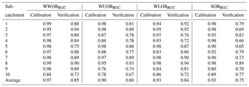
The soil moisture data fused using the WKNN model exhibits enhanced timeliness, with the soil moisture in each conceptual soil profile aligning closely with that of the CLDAS data (Table 3). Specifically, during the calibration set, the correlation coefficients with CLDAS data consistently exceed 0.9. Additionally, the correlation coefficients in the validation set are 0.85, 0.80, 0.84, and 0.75, respectively, indicating that the WKNN model possesses robustness and generalizability. It effectively captures the statistical relationship between point-scale and areal-scale soil moisture datasets.

Table 3 The correlation coefficient between the fused soil moisture data and CLDAS soil moisture data.

5.2.2 Multivariate observation assimilation scheme

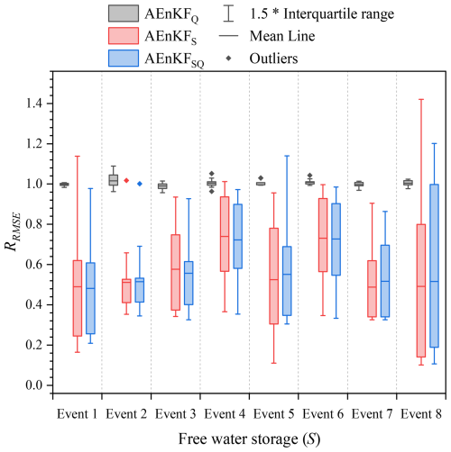
Within the context of one-step prediction, Fig. 8 displays the impact of updating free water storage in three different assimilation schemes, quantified by R_RMSE. For the AEnKF_Q scheme, there is no update to free water storage, leading to expected R_RMSE values oscillating near 1.0. Conversely, both AEnKF_S and AEnKF_SQ successfully updated free water states, with mean values of R_RMSE for free water storage in flood event simulations lying between 0.48 and 0.74. This demonstrates an average reduction in RMSE of 26 % to 52 % for free water storage across various flood events in comparison to the OL mode. Moreover, Fig. 8 reveals that, in the vast majority of cases, the whiskers (representing 1.5 times the interquartile range) of the red and blue boxes remain below 1.0. This indicates that both AEnKF_S and AEnKF_SQ successfully updated the free water storage in most sub-catchments for most flood events. The effective updates to free water storage will further impact the discharge process at the catchment outlet, which is discussed in detail in the subsequent sections.

Figure 8 Effects of three assimilation schemes on free water storage (S).

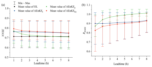
We evaluate the optimal single-value performance of the AEnKF in one-step (1 h) prediction. Figure 9 illustrates the NNSE and R_RMSE values achieved through three AEnKF assimilation schemes. In OL, the mean NNSE stands at 0.75. Following assimilation with three schemes, the mean values of NNSE improve to be 0.79, 0.78, and 0.81, respectively. The R_RMSE of AEnKF_Q fluctuates between 0.78 and 1.0, with an average of 0.88; for AEnKF_S, it ranges from 0.71 to 1.02, averaging 0.91; and for AEnKF_SQ, it varies from 0.64 to 0.99, with an average of 0.84. These results show that all three AEnKF assimilation schemes enhance the optimal single-value performance, with AEnKF_SQ outperforming AEnKF_Q, which in turn exceeds AEnKF_S. Moreover, AEnKF_SQ achieves a higher improvement ceiling in certain flood events. For instance, the maximum reduction in RMSE reaches 22 % for AEnKF_Q, 29 % for AEnKF_S, and up to 36 % for AEnKF_SQ.

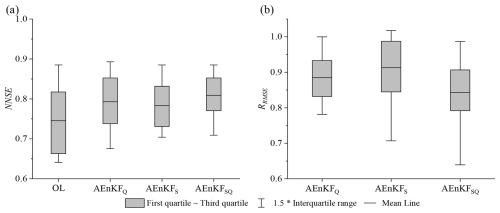
Figure 9 The optimal single-value performance of three AEnKF assimilation schemes for real-world cases for (a) NNSE and (b) R_RMSE.

Figure 10 utilizes R_CRPS and R_RELI metrics to evaluate overall ensemble performance and reliability. The R_CRPS values for AEnKF_Q are in the range of 0.81 to 1.0, averaging at 0.90; for AEnKF_S, they span from 0.71 to 1.02, averaging 0.92; and for AEnKF_SQ, they vary from 0.66 to 0.98, averaging 0.86. Notably, AEnKF_Q exhibits the narrowest box plot, indicating a more focused distribution of R_CRPS for this scheme. The average R_CRPS for AEnKF_S closely aligns with that of AEnKF_Q, yet its box plot shows greater breadth at both the top and the bottom, suggesting a higher potential for improvement in overall ensemble performance but with increased instability. In contrast, the average R_CRPS for AEnKF_SQ is lower than those of the first two. While the box plot width for AEnKF_SQ is similar to that of AEnKF_S, the upper boundary of the box plot aligns more closely with AEnKF_Q, and the upper whisker is shorter than that of AEnKF_Q, indicating a comprehensive superiority of AEnKF_SQ in overall ensemble performance compared to both AEnKF_S and AEnKF_Q. Similar findings also emerge in the assessment of ensemble reliability. AEnKF_S and AEnKF_Q exhibit similar mean R_RELI values, but the box plot for AEnKF_Q is more constricted. In contrast, AEnKF_SQ shows a thorough superiority in ensemble reliability compared to both AEnKF_S and AEnKF_Q.

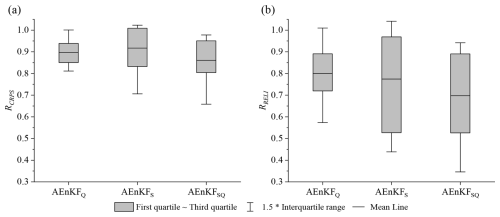
Figure 10 The ensemble performance of three AEnKF assimilation schemes for real-world cases: (a) R_CRPS and (b) R_RELI.

We extend the examination to the temporal persistence of assimilation effects for these schemes. Figure 11 displays discharge forecasting accuracy across various lead times, as measured by NNSE and R_RMSE. Within a lead time range of 1 to 8 h, both AEnKF_S and AEnKF_SQ demonstrate improvements in forecasting performance: AEnKF_SQ exceeds AEnKF_S within both lead times. AEnKF_Q shows significantly shorter temporal persistence than the other two, slightly outperforming AEnKF_S in 1 h lead time but with a rapid decline in accuracy as lead time increases. Past a 5 h lead time, the assimilation effect of AEnKF_Q vanishes, leading to accuracy slightly below OL. And at different lead times, AEnKF_SQ consistently outperforms AEnKF_Q. This reveals that employing AEnKF for updating cumulative channel flow may notably enhance discharge forecasting accuracy in shorter lead times. While updating free water storage may not be as effective as AEnKF_Q initially, it ensures a longer-lasting assimilation impact. The scheme of AEnKF_SQ merges these strengths, offering robust discharge corrections and an extended temporal persistence of assimilation effects.

Figure 11 The accuracy of forecasted discharge under different lead times for (a) NNSE and (b) R_RMSE.

6 Discussion

6.1 Discussion of AEnKF time window in synthetic cases

In the study of assimilation windows for the AEnKF in synthetic cases, we found that longer assimilation windows do not necessarily yield better results (Fig. 3). This is primarily because a longer time window includes too much historical information, which may have a weak correlation with the current state variables. Due to the non-linearity of the hydrological model, where overly long windows can result in the system assimilating excessive noise, which negates the benefits derived from incorporating past observations. Tao et al. (2016) obtained similar results when studying the assimilation window length (1–3 h) for the assimilation of observed discharge only. They found that the 2 h time window generally yielded better assimilation results than the 3 h time window, while the 1 h time window performed the worst.

6.2 Discussion of two flood events in real-world cases

In flood simulation and forecasting, peak flow rates are a primary focus for researchers. Using the two flood events with the most significant peak flow errors in the OL mode in 2023 (no. 2023040308 and no. 2023052008) as case studies, we examined the variations in free water storage and discharge at the catchment outlet.

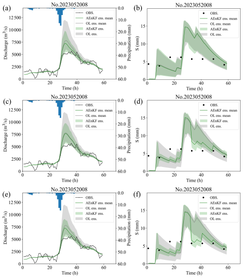
Figure 12 displays the hydrographs simulated for no. 2023040308. Black lines (and dots) signify observed values. Grey lines and bands represent the ensemble mean and range of OL, respectively. Similarly, green lines and bands illustrate the ensemble mean and range for the AEnKF. In examining the time series of free water storage, it is evident that observational data points almost never fall within the grey bands of the OL scheme. This indicates a notable difference between the soil moisture levels simulated by the Xin'anjiang model and those derived from observational data. Both AEnKF_S and AEnKF_Q exhibit similar update patterns, where the post-update ensemble mean values significantly shift towards observational data. Concurrently, this adjustment expands the ensemble bands, indicating an increase in ensemble simulation accuracy for AEnKF_S and AEnKF_Q along with an increased ensemble spread. In the analysis of the discharge time series, it becomes evident that the ensemble distribution from the AEnKF aligns more closely with observational data and presents a narrower bandwidth than that of OL. This trend suggests that the ensemble accuracy with the AEnKF exceeds that of the OL scheme and also demonstrates a reduced ensemble spread. Furthermore, the ensemble distribution observed during peak periods is more expansive than during the onset and recession periods of flood. This is attributed to the error models applied. These models introduce larger perturbations in the assimilation system during peak periods, leading to a broader ensemble distribution, which, in turn, ensures a more effective assimilation during these critical periods. In examining the time series of discharge, it is noted that both AEnKF_Q and AEnKF_S significantly reduced the height of the simulated flood peak. The AEnKF_Q scheme shows effectiveness around the 20th hour, following the assimilation of approximately 20 discharge observations, achieving a relative error of 17 % in the simulated flood peak (maximum instantaneous flow) compared to the observed peak. AEnKF_S started effectively updating the discharge following the assimilation of the third group of soil moisture observations at the 17th hour, which led to a flood peak relative error of 13 %. The AEnKF_SQ scheme successfully amalgamates the strengths of both, culminating in a reduced flood peak relative error of merely 8 %.

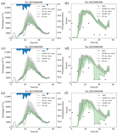
Figure 12 Hydrograph during flood event labeled no. 2023040308 for the (a, b) AEnKF_Q scheme, (c, d) AEnKF_S scheme, and (e, f) AEnKF_SQ scheme. The left panels show the discharge at the catchment outlet, and the right panels display the free water storage in sub-catchment 1.

In the case of the flood event labeled no. 2023052008, as illustrated in Fig. 13, the time series exhibits a similar pattern to no. 2023040308. The peak flooding occurred between the 25th and 33rd hours, which corresponds to the period between the fourth and fifth sets of soil moisture observations. During this interval, there is a notable and rapid increase in free water storage. Figure 13c indicates that the AEnKF_S fails to effectively adjust the discharge volumes around the peak period. Conversely, the AEnKF_Q scheme, which focused on updating cumulative channel flow, successfully rectified the peak flooding. Owing to the ineffectiveness of free water content updates in discharge correction, the assimilation impact of AEnKF_SQ closely matched that of AEnKF_Q. In summary, it is apparent that AEnKF_SQ effectively integrates the strengths of both the AEnKF_S and AEnKF_Q schemes. Even when one of these strategies fails to update effectively, AEnKF_SQ still manages to enhance the precision of discharge predictions.

Figure 13 Hydrograph during flood event labeled no. 2023052008 for the (a, b) AEnKF_Q scheme, (c, d) AEnKF_S scheme, and (e, f) AEnKF_SQ scheme. The left panels show the discharge at the catchment outlet, and the right panels display the free water storage in sub-catchment 1.

6.3 Limitations

The Xin'anjiang model is a conceptual hydrological model that generalizes the rainfall–runoff process. Its most prominent feature is performing runoff production calculations based on the saturation-excess runoff mechanism, meaning net rainfall is first entirely used to replenish soil water, and once the soil moisture content in the unsaturated zone reaches field capacity, all subsequent net rainfall is used to generate runoff. Therefore, the Xin'anjiang model is mostly suitable for humid and semi-humid regions where the saturation-excess runoff mechanism is dominant and is less or not applicable to arid and semi-arid regions. However, it is important to note that the state updating method proposed in this study is not limited to coupling with the Xin'anjiang model. In fact, this method can be easily coupled with any lumped or semi-distributed hydrological model that includes state variables related to soil moisture and channel storage. When coupled with hydrological models suitable for semi-arid and arid regions, it can be effectively applied in those areas.

Semi-distributed hydrological models, like the Xin'anjiang model used in this study, have smaller state variable dimensions, allowing for the direct application of the proposed state updating scheme. However, in distributed models where each computational grid (e.g., DEM-based grids) has its own state variables, the state dimension becomes large, making direct application inefficient or prone to spurious correlations from distant observations. To resolve this, we recommend applying covariance localization (Janjić et al., 2011) to the AEnKF or other localization techniques (Khaniya et al., 2022). For instance, in covariance localization, a localization radius (RL) is set, and the forecast error covariance matrix is adjusted using a correlation matrix derived from the Schur product theorem. This study focuses on jointly assimilating soil moisture and streamflow using the AEnKF, and performing localization on the AEnKF is beyond the scope of this research. We will explore this further in future work.

Real-time flood forecasting is a dynamic prediction system based on real-time monitoring data combined with hydrological and/or hydrodynamic models to predict the evolution of flood processes. It provides critical information such as the time of peak flow, water levels, and discharge when a flood occurs. This type of forecasting is characterized by its high timeliness and short forecasting window, with the lead time generally set to several hours (e.g., Toth et al., 2000; Liu et al., 2016). The methods proposed in this study is particularly suited for state updating within real-time flood forecasting as it dynamically updates the state variables of the hydrological model using real-time observational data, reducing the accumulation of errors. In real-world cases, we set the maximum lead time to 8 h, which sufficiently meets the requirements for real-time flood forecasting in medium-sized catchments. This provides reliable real-time and near-real-time information for emergency responses, assisting government and flood control agencies in organizing evacuations, resource allocation, and reservoir operations, thereby minimizing casualties and property damage caused by floods. Moreover, to test the temporal persistence of the state updating method, we used historical observed rainfall as a perfect proxy for numerical weather forecasts, thereby avoiding the introduction of uncertainties from numerical weather predictions. As the lead time increases, uncertainties in numerical weather predictions may gradually replace the accumulation of errors in hydrological model state variables as the primary source of uncertainty in flood forecasting (Weerts and El Serafy, 2006; Yossef et al., 2013; Thiboult et al., 2016). For medium- to long-term flood forecasts, greater attention may need to be given to uncertainties stemming from numerical weather predictions.

7 Conclusions

This study uses the asynchronous ensemble Kalman filter (AEnKF) with enhanced error models for assimilating two types of observational data into the Xin'anjiang model. The data include observed discharge at catchment outlet and soil moisture gathered from multiple sources. The objective is to diminish error accumulation in the initial conditions of the Xin'anjiang model at the start of flood forecasting, thereby enhancing initial conditions. The assimilation framework includes advanced error models, such as the BGEM model to reduce systematic biases from perturbed soil moisture and the MAP method for the objective estimation of hyperparameters in the error model. The study specifically contrasts three AEnKF assimilation strategies: (1) the AEnKF_Q scheme, which updates cumulative channel flow in the Xin'anjiang model by assimilating observed outlet discharge; (2) the AEnKF_S scheme, which focuses on updating soil moisture variables in the model by assimilating fused soil moisture observations; and (3) the AEnKF_SQ, a joint assimilation scheme, which combines both discharge and soil moisture assimilation processes.

Generally, the AEnKF is considered an effective approach for updating hydrological model states. It integrates a greater amount of observational data while barely increasing the computational burden, making it highly suitable for flood forecasting. The effectiveness of assimilation with the AEnKF relates to the assimilation time window. Results for synthetic data cases indicate that an appropriate setting involves a 3 h time window for assimilating observed soil moisture and outlet discharge. Moreover, in lead times ranging from 1 to 24 h, this method consistently outperforms the EnKF approach.

In synthetic case studies, while updating soil moisture state variables of the Xin'anjiang model, it is observed that effective updates are limited to free water storage and total tension water storage. This underscores the significance of choosing appropriate state variables for updates in the application of the AEnKF method. Further analysis revealed that with high-quality hourly available observational data, all three assimilation schemes maintained their effectiveness for up to 24 h lead time. Notably, AEnKF_SQ demonstrated enhanced optimal single-value performance, overall ensemble performance, and ensemble reliability, surpassing both AEnKF_S and AEnKF_Q. Specifically, in the one-step forecast, the MR_RMSE for AEnKF_SQ decreased by 0.11 and 0.16 compared to AEnKF_S and AEnKF_Q, respectively; the MR_CRPS for AEnKF_SQ decreased by 0.10 and 0.15, and the MR_RELI decreased by 0.20 and 0.15 compared to AEnKF_S and AEnKF_Q, respectively. AEnKF_SQ's advantage in optimal single-value performance persists up to a 24 h lead time.

In the real-world case studies, we merged soil moisture data from in situ monitoring sites with the near-real-time CLDAS soil moisture data. This fusion produces spatially distributed data characterized by high temporal immediacy while addressing the limitation of point-scale in in situ soil data. In contrast to experiments using synthetic data, extending soil moisture observation intervals to 8 h impacts the performance of the AEnKF_S scheme. In one-step prediction, the AEnKF_SQ scheme exhibits the highest level of accuracy with the MR_RMSE of 0.84. Concurrently, the simulation precision of the AEnKF_Q scheme exceeds that observed in AEnKF_S, with MR_RMSE values of 0.88 and 0.91, respectively. Variations in results are observed under different lead times. AEnKF_SQ and AEnKF_S consistently demonstrate an assimilation effect duration of 8 h in contrast to the 5 h temporal persistence of the assimilation effect of AEnKF_Q. The use of the AEnKF for updating cumulative channel flow markedly enhances the accuracy of discharge forecasting in a brief lead time. In contrast, the adjustment extent of discharge by updating free water storage in a single-step forecast might be lower than that achieved with AEnKF_Q. Nevertheless, it guarantees a more sustained assimilation effect. The AEnKF_SQ integrates the strengths of the previous two strategies, thereby improving discharge forecasting accuracy even when a particular strategy does not update effectively and prolonging the temporal persistence of the assimilation effect.