Quantitative soil characterization using the frequency domain electromagnetic induction method in heterogeneous fields

The frequency domain electromagnetic induction (FDEM) method is a widely used tool for geophysical soil exploration. Field surveys using FDEM provide apparent electrical conductivity (ECa), which is typically used for qualitative interpretations. Quantitative estimations of soil properties remain challenging, especially in heterogeneous fields. Quantitative approaches are based on either deterministic or empirical modeling. While the deterministic approach faces limitations related to instrumental drift, data calibration, inversion, and pedophysical modeling, the empirical approach requires developing a local model, which involves extensive field sampling.

This study aims to evaluate the effectiveness of FDEM modeling based on either a deterministic or empirical approach, identify its limitations, and search for optimal field protocols. We provide practical guidelines for end users to quantitatively predict soil water content, bulk density, clay content, cation exchange capacity, and water EC in heterogeneous fields. Two field surveys were conducted in Belgium, where FDEM data were collected using Dualem-421S and Dualem-21HS sensors, along with data taken from electrical resistivity tomography (ERT) measurements and an impedance moisture probe and soil sampling. A comprehensive sensitivity analysis revealed that deterministic modeling procedures could not predict water content more accurately than a mean value approximation (negative R²). This analysis also highlighted the sensitivity of the minimization method used in FDEM data inversion and the applied pedophysical model. Empirical modeling, which does not require FDEM data calibration or inversion, outperformed the deterministic approach. However, its prediction accuracy is limited, particularly if soil sample depth is not considered.

1 Introduction

Frequency domain electromagnetic induction (FDEM) tools are widely applied in geophysical soil surveys (Boaga, 2017). These instruments often serve to qualitatively determine spatiotemporal changes in the apparent electrical conductivity (EC_a), reflecting the influence of soil characteristics within the measured soil volume (Doolittle and Brevik, 2014). As the relationship between electrical conductivity (EC) and several of such soil attributes has been investigated extensively, FDEM is also capable of their quantitative assessment. Specifically, soil water content is a preferred target because of its central role in soil–plant interaction, groundwater assessment, soil ecological functioning, and climate regulation.

Despite these applications, a broader practical implementation of FDEM remains mainly limited to academic settings (Altdorff et al., 2017; Huang et al., 2007). Two major challenges hinder wider adoption. Firstly, the FDEM methodology itself faces issues such as instrumental drift, approximations to translate raw FDEM data to EC_a, calibration difficulties (Hanssens et al., 2020; Minsley et al., 2012), and the necessity for data inversion of EC_a to true EC before a non-local quantitative assessment can be made. This reality persists even though – particularly for research purposes – adaptive correction procedures and open-source inversion codes have become available. Secondly, a significant obstacle in translating soil EC data into a target soil property lies in the current limitations of pedophysical models. These models are non-site-specific deterministic and link geophysical variables with soil properties (see, e.g., Friedman, 2005; Glover, 2015; Romero-Ruiz et al., 2018) but often suffer from a lack of precision and are difficult to generalize. This is exacerbated by the variability in soil types, spatial heterogeneity, temperature conditions, and the electromagnetic frequency of measurements (Jougnot et al., 2018; Moghadas and Badorreck, 2019). Importantly, the difference between the laboratory-analyzed and FDEM-measured soil volumes can cause scale inconsistencies (Lück et al., 2022) that affect the validity of these relationships. As an alternative to pedophysical models, field-specific empirical relationships can be composed at the cost of obtaining significant amounts of calibration data (Corwin and Lesch, 2003). Despite empirical modeling being inherently limited to the conditions represented by the dataset the model has been trained for, exhaustive assessments of this method demonstrated useful predictions of various soil properties across agricultural fields (Boaga, 2017; Rentschler et al., 2020).

Here, we evaluate how FDEM data can serve to quantitatively predict spatial variations in volumetric soil water content (θ), bulk density (ρ_b), clay content, cation exchange capacity (CEC), and water EC (EC_w) in a practical, straightforward manner on two heterogeneous test sites. In search for optimal field protocols, we evaluate to which extent considering instrumental limitations and different procedures of FDEM data correction and processing influences the accuracy of the predicted soil attributes and what the trade-off between deploying a physics-driven deterministic versus field-specific data-driven model implies. Finally, we propose field and modeling strategies for optimal soil characterization with FDEM surveys.

2 Methodology

2.1 FDEM functioning

FDEM devices function by passing an alternating current through a transmitter coil, creating a oscillating primary electromagnetic field that varies over time. This primary field (H_P) interacts with the subsurface, inducing eddy currents which subsequently produce a secondary electromagnetic field (H_S). The $H_{\mathrm{S}}/H_{\mathrm{P}}$ ratio is detected by the receiver coil and is quantified as a complex number, consisting of an in-phase component (IP = Re($H_{\mathrm{S}}/H_{\mathrm{P}}$)) and a quadrature component (QP = Im($H_{\mathrm{S}}/H_{\mathrm{P}}$)). Both IP and QP are typically measured, reflecting the device setup and the conditions of the subsurface.

The QP expressed in parts per million (ppm) can be converted to the actual EC_a using the linear model developed by McNeill (1980) assuming a homogeneous subsurface electrical conductivity. This model assumes a uniform subsurface EC and is known as the low induction number (LIN) approximation. It is valid when the induction number (β) is low (β≪1). The LIN approximation proposed by McNeill (1980) is given by

$$\begin{array}{}\text{(1)}& {\mathrm{EC}}_{\mathrm{a}}=\mathrm{QP}{\displaystyle \frac{\mathrm{4}}{{\mathit{\mu }}_{\mathrm{0}}\mathit{\omega }{s}^{\mathrm{2}}}}\text{when}\mathit{\beta }=s\sqrt{{\displaystyle \frac{{\mathrm{\mu }}_{\mathrm{0}}\mathit{\omega }\mathrm{EC}}{\mathrm{2}}}}\ll \mathrm{1},\end{array}$$

where ω is the angular frequency, μ₀ is the magnetic permeability of free space ($\mathrm{1.257}\times {\mathrm{10}}^{-\mathrm{8}}$ H m⁻¹), and s is the coil separation. It can be seen from this equation that large frequencies and higher EC soils will violate the β≪1 specification. It is important to note that the LIN approximation also assumes that the FDEM device is operated at ground level above a homogeneous, poorly conductive subsurface (Callegary et al., 2007; McNeill, 1980).

2.2 Data collection

Two heterogeneous agricultural fields were examined in this study. Site 1, located in Middelkerke, Belgium, is shown in Fig. 1a. Belgian soil map data (Van Ranst and Sys, 2000) indicate that the field is affected by saline groundwater and exhibits a soil texture varying from loam (26 % clay, 34 % sand) to silt loam (10 % clay, 40 % sand) (USDA textures), with clay layers starting at depths greater than 0.50 m. In contrast, Site 2, located in Bottelare, Belgium (Fig. 1b), is characterized by fresh groundwater. The soil texture at this location ranges from sandy loam (13 % clay, 76 % sand) to clay (64 % clay, 5 % sand). Both sites have a plow horizon, are actively used for agriculture, and had no standing crops at the time of the survey.

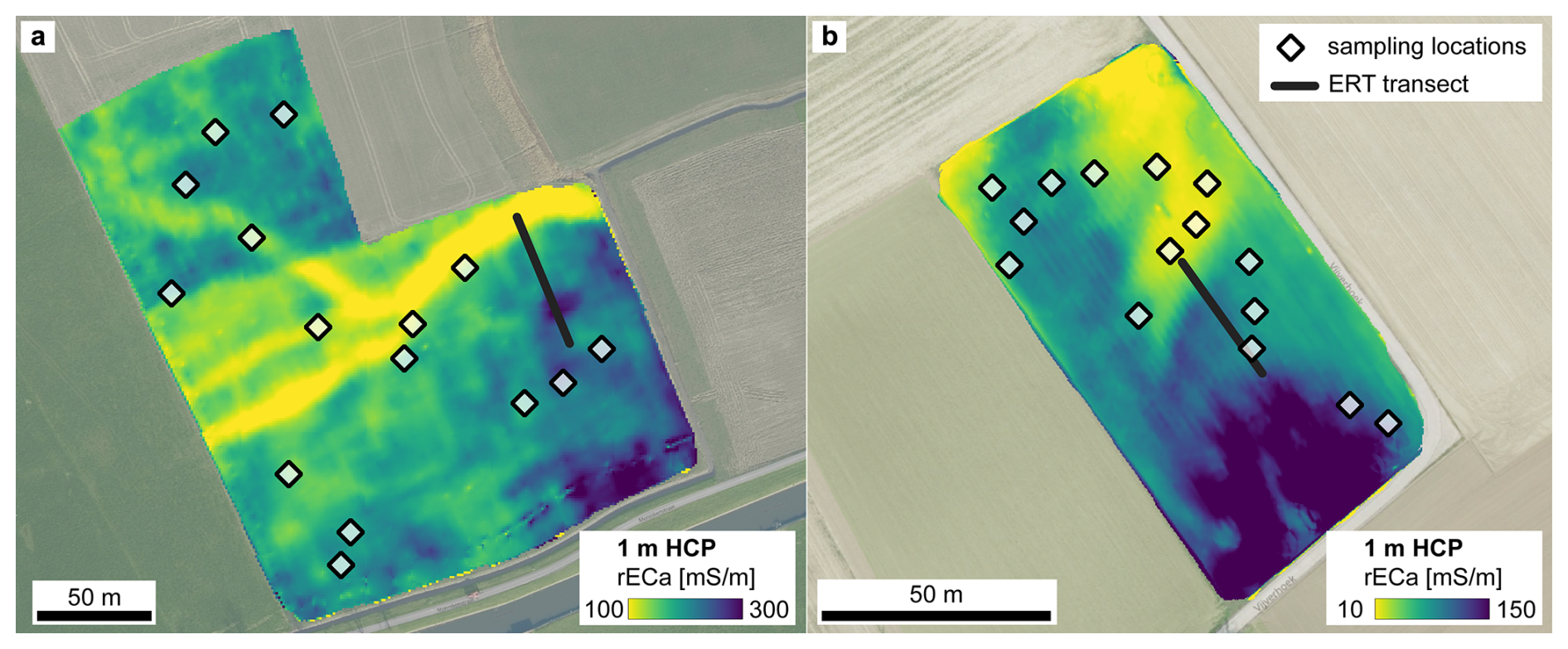
Figure 1 Site 1 in Middelkerke (a) and Site 2 in Bottelare (b) (Belgium), with the position of the ERT transects and 15 soil sampling locations per site, selected via conditioned Latin Hypercube Sampling based on previously obtained FDEM LIN EC_a data. The mapped data are ERT-calibrated robust EC_a HCP1.0.

Field surveys at both sites involved collecting FDEM data using different sensors, all operating at 9 kHz: the Dualem-421S at Site 1 with a 3 m crossline sampling density and the Dualem-21HS at Site 2 with a 1 m crossline sampling density, both with a constant distance above ground of 0.165 m using a sled. The instrument was pulled with a quad across the field with a driving speed of approximately 10 km h⁻¹ and a measurement sampling rate of 10 Hz. The crossline sampling density was decided based on the time to survey each field, Site 1 being bigger. The surveys at both sites provided in-phase (IP) and quadrature-phase (QP) data with an in-line sampling density of approximately 0.3 m in horizontal co-planar (HCP) and perpendicular (PRP) configuration. For both sites, transmitter–receiver separations of 1.0 m (HCP1.0), 1.1 m (PRP1.1), 2.0 m (HCP2.0), and 2.1 m (PRP2.1) were used. Additionally, 4.0 m HCP (HCP4.0) and 4.1 m PRP data (PRP4.1) were collected at Site 1 and 0.5 m HCP (HCP0.5) and 0.6 m PRP data (PRP0.6) at Site 2. Electrical resistivity tomography (ERT; Syscal Pro, Iris Instruments) was performed with 0.5 m electrode spacing, during the FDEM surveys (Fig. 1). The ERT transects were located based on previous surveys to include the largest EC_a range across the field.

In addition to geophysical surveys, soil sampling was carried out at 15 predetermined locations at each site. These locations were strategically selected using the Latin hypercube sampling method (Minasny and McBratney, 2006) and were based on insights from previously collected FDEM data. Undisturbed soil samples were extracted from two depths, 0.10 m (topsoil) and 0.50 m (subsoil) below the surface, in stainless steel 100 cm³ cores using an auger. In total, 30 samples per site were analyzed in the laboratory to obtain soil texture (after sieving at 2 mm), CEC (CoHex method, Ciesielski et al., 1997a, b), θ, and ρ_b (gravimetric method with convective oven drying at 105 °C).

To accurately determine in situ EC, EC_w, and temperature within the soil sampling volume (100 cm³), measurements were taken at each sampling location using a HydraProbe soil probe (HydraProbe, Stevens Water Monitoring Systems, 2008). The correction proposed by Logsdon et al. (2010) was applied to improve the quality of these EC readings.

2.3 Data processing

The general processing workflow of the FDEM survey follows Hanssens et al. (2020) and is described in Fig. 2. The methodology aims at processing the FDEM data to obtain reliable EC data at sampling locations and then predict soil properties. For this process, a meaningful physical modeling sequence was followed. For instance, no inversion was implemented on uncalibrated FDEM data. This involved four key steps: ERT inversion, FDEM data calibration, FDEM data inversion, and pedophysical modeling (Hanssens et al., 2020). All computer code used is open-source, and default parameters were prioritized, ensuring reproducibility of methodology and results. All developed codes for this section are available in Mendoza Veirana (2024b) and collected data in Mendoza Veirana (2024a).

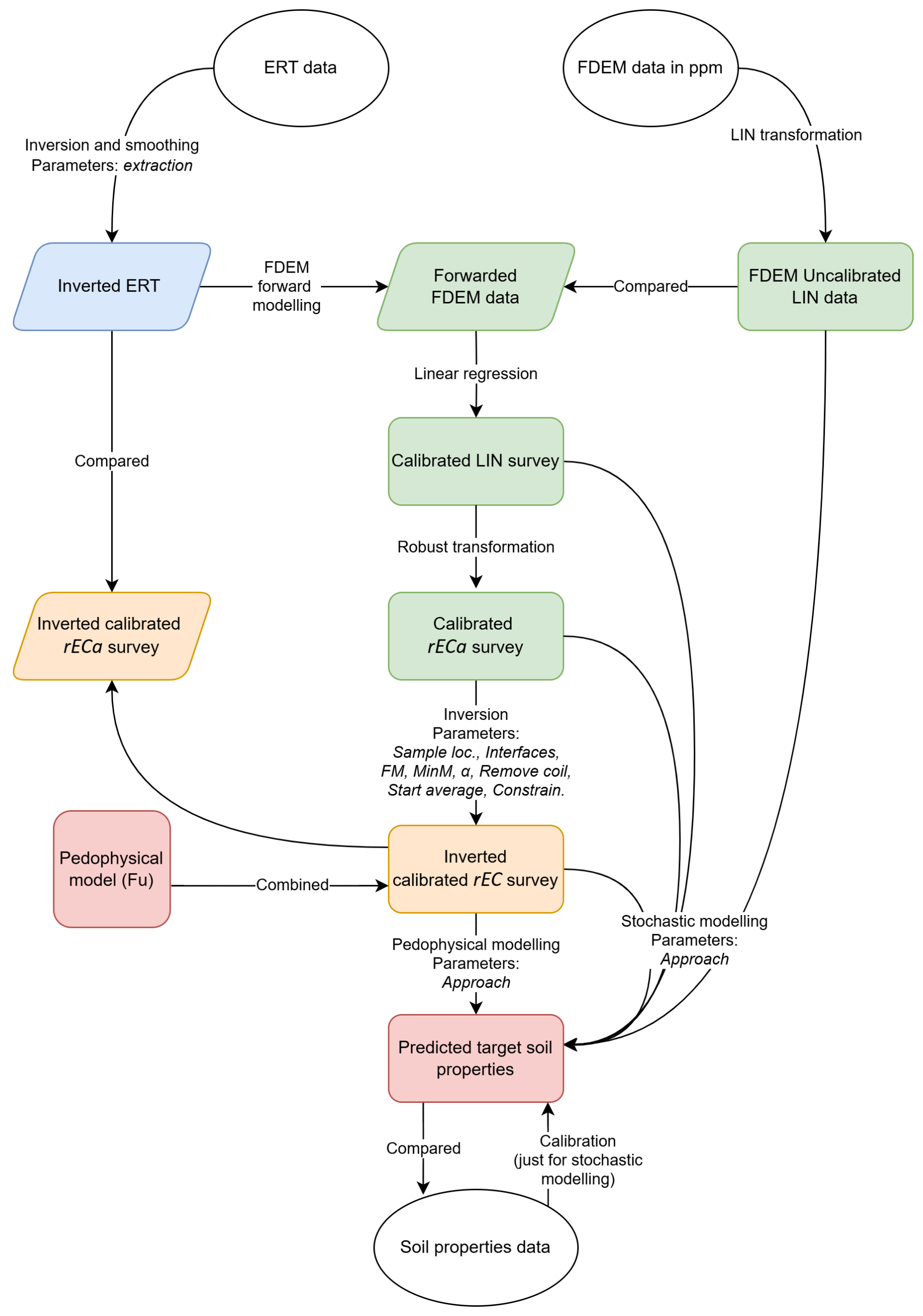
Figure 2 Workflow of geophysical data process including prediction of soil properties. Ellipses represent observations that exist independently of all data processes. Rectangles represent data over all the field and/or soil sampling locations. Parallelograms represent data over the ERT profiles. The square represents an external model. Colors represent modeling processes: light blue for ERT inversion (Jupyter Notebook “00_inv-ERT”), green for FDEM data calibration (Jupyter Notebook “01_QP_ cal”), orange for FDEM data inversion (Jupyter Notebook `02_EC_invert'), and red for soil properties modeling (Jupyter Notebook “03_Soil_properties_modelling”).

2.3.1 ERT inversion

The measured ERT data were inverted using the ResIPy (v3.5.4) open software (Blanchy et al., 2020) which is based on the R2 codes (Binley and Kemna, 2005) (see Fig. 2 light-blue box; see full code in the Jupyter Notebook “00_inv-ERT”). The method for inversion follows a least-squares minimization between the measured ERT data and modeled subsurface geoelectrical parameters. The inversion process incorporates regularization techniques that balance data fidelity and smoothness of the subsurface model to address the inherent non-uniqueness and instability in ERT data inversion (Binley, 2015). A standard inversion using a triangular mesh was implemented, converging after three iterations. After inversion, extraction of ERT profiles was done by averaging the EC in a neighborhood of 0.5 m around each electrode. Alternatively, to obtain smoother profiles, an extraction window of 2.5 m was also used.

2.3.2 FDEM data calibration

Calibrating raw FDEM data is required for obtaining reliable EC data at sampling locations, and such calibration was done by combining ERT and FDEM data (see Fig. 2, green boxes) (Lavoué et al., 2010; van der Kruk et al., 2018). On the one hand, the raw uncalibrated FDEM data (in ppm) were transformed to EC_a data following the LIN approximation. On the other hand, the inverted ERT EC data were firstly grouped by profile, and any profiles at the beginning or end of each transect that did not reach a minimum depth of 4 m were removed due to the lower sensitivity in those peripheral zones. After this, 100 profiles remained for Site 1 and 40 profiles for Site 2. Subsequently, the inverted ERT profiles were forward-modeled to the theoretical FDEM LIN EC_a measured by the Dualem instrument over the ERT transect (Lavoué et al., 2010). The forward model implements a 1D full solution of Maxwell's equations considering an electromagnetic field, which, after FDEM instrument reading, is composed by IP and QP signals.

After calculating both FDEM LIN EC_a data over the ERT profiles, these data were matched by spatial proximity with the closest FDEM data point. A linear regression was then fitted for the six coil configurations (see Fig. 3). This linear regression was applied to the entire FDEM survey dataset, effectively performing a linear calibration.

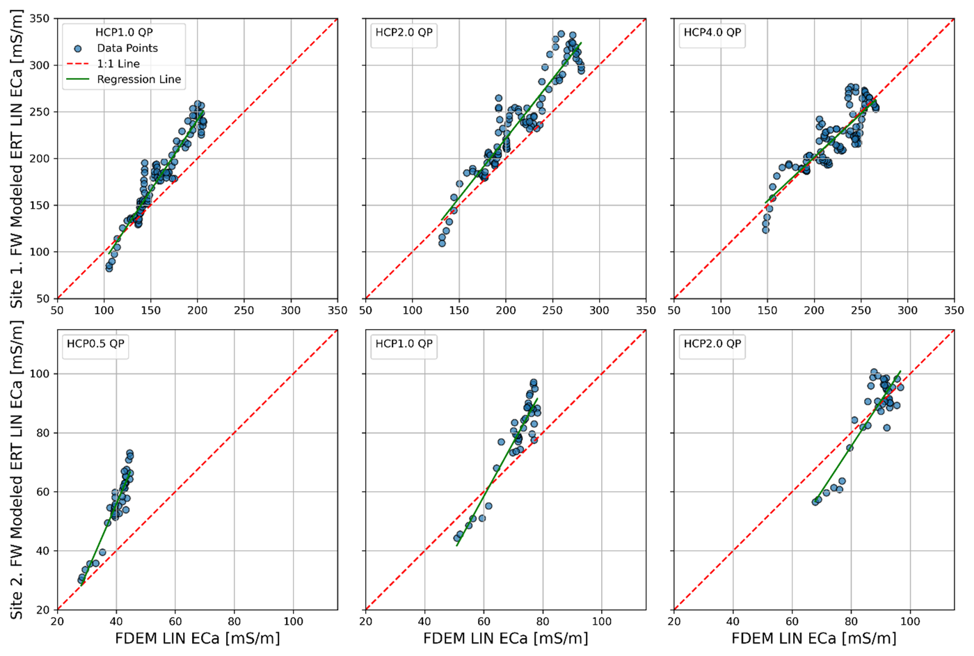
Figure 3 Calibration of FDEM QP data. A linear regression is fit between the FDEM LIN EC_a data collected on the field (X axis) over the ERT transect and the FDEM response that was forward-modeled from the inverted ERT data (Y axis). This is shown for the three different QP coil configurations across the three subplot columns and for both sites displayed in the top and bottom rows.

Lastly, the calibrated FDEM QP data were transformed to robust EC_a (rEC_a) values to provide reliability beyond LIN constraints (Hanssens et al., 2019), such as high salinity and clay content levels. A visual comparison of the forwarded FDEM EC_a and uncalibrated and calibrated LIN and rEC_a FDEM data over the ERT transect is shown in Fig. 4. The rEC_a consistently exceeds the LIN EC_a, reflecting the known limitations of the LIN approach and aligning with the tests reported by Hanssens et al. (2019).

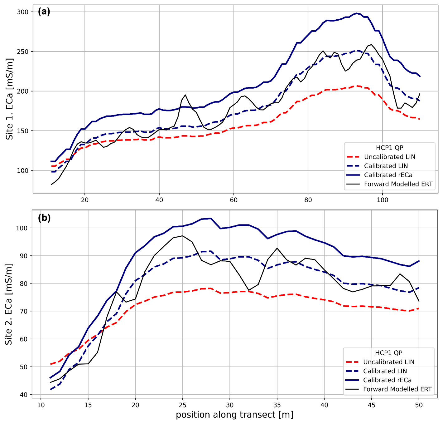
Figure 4 Comparison of HCP1.0 QP EC_a data along the ERT transect for Site 1 (a) and Site 2 (b). This includes calibrated and uncalibrated FDEM (LIN) EC_a and calibrated robust (rEC_a) data. Also, the forward-modeled ERT (LIN) EC_a data are shown.

2.3.3 FDEM data inversion

To assess the impact of the different modeling steps, we provide the parameters used and alternatives for comparison. To obtain top- and subsoil EC, 1D data inversion was performed with EMagPy (v1.2.2) (McLachlan et al., 2021) using the full Maxwell-based forward model (Wait, 1982). For both sites and based on borehole observations, a five-layer subsurface discretization was maintained, with fixed interfaces at 0.3, 0.6, 1.0, and 2.0 m. Another option for layer interfaces definition consists in using a logarithmic scale from 0.15 to 2.0 m. The closest FDEM observation to each sampling location was selected as the reference, in contrast to averaging FDEM observations within a radius (2 m for Site 1 and 1 m for Site 2) around the sampling location. Additional parameters of the inversion problem include an optimization method (Gauss–Newton) (Virtanen et al., 2020) or Robust Parameter Estimation (ROPE) (Bárdossy and Singh, 2008), a vertical smoothing parameter (α, default = 0.07), and L2 norm objective function. Moreover, inversion data were composed of all the coil configurations. Removing HCP2.0 and PRP2.1 for Site 1 and HCP0.5 and PRP0.6 for Site 2 could lead to lower inversion errors. The starting model for inversion was set to the average of the ERT profiles using the given subsurface layers; alternatively, one particular reference ERT profile can be used. Inversions with a negative R² error were discarded and not analyzed further. Finally, EC limits (constraints) were applied to rEC_a FDEM data at sampling locations during its inversion process (just for ROPE solver). These were defined as the minimum and maximum EC values of the inverted ERT profiles.

Once the EC data were obtained by inversion of the rEC_a FDEM data for each sample location, they were used to calculate the soil properties of interest.

2.3.4 Soil property calculation

Linking EC data to soil properties at sampling locations can follow two basic modeling strategies: local empirical and universal deterministic modeling.

Local empirical modeling enables us to empirically predict several soil properties across the surveyed field, at the expense of collecting and analyzing soil samples to build a training dataset. This modeling consists of fitting functions to the training dataset and predicting at targeted locations. Traditionally, polynomial functions have been used for this task (Rentschler et al., 2020), but in recent years machine learning algorithms (such as artificial neural networks and random forest) have performed better (Moghadas and Badorreck, 2019; Rentschler et al., 2020; Terry et al., 2023). However, using machine learning requires a large number of training data that may not be obtainable for practical FDEM applications. Thus, we stick to polynomial functions for empirical modeling.

In our case, for both sites the original soil analysis dataset (n=30) was randomly split into a training dataset (n=20), while the remaining was used as test dataset (n=10); this process was repeated 100 times. The optimal polynomial degree was chosen as the one that maximizes the median R² errors on all the 100 test sets.

Three distinct approaches to polynomial development were utilized. A first approach, named “layers together” (ST-LT), consisted of combining data from different soil depths so that no differentiation was made between top- and subsoil samples for model development. Secondly, these sample sets were considered separately in an approach whereby different polynomials were developed for each soil layer (“layers separate”(ST-LS)). In this modeling approach, the same polynomial degree was maintained for both top- and subsoil data. Finally, the ST-LS2 approach was like ST-LS but permitted different polynomial degrees for the models of each layer.

Model training features included calibrated (LIN and robust) and uncalibrated (LIN) EC_a data from the six FDEM coils and the inverted EC data at soil sampling locations, while independent targeted soil properties were θ, cation exchange capacity (CEC), clay content, ρ_b, and EC_w.

Deterministic modeling uses general pedophysical EC–θ relationships based on physical principles that have been validated across a wide range of soil conditions (e.g., models presented by Rhoades et al., 1976). Such modeling does not require calibration data, avoiding the cost of field sampling and laboratory analysis. However, such pedophysical models may fall short in representing extreme scenarios outside the tested soil characteristics ranges. Additionally, soil data (such as porosity, EC_w, and texture) must be available to adequately populate the model and predict the target property. Lastly, soil data also require corrections of temperature and electromagnetic frequency (Moghadas and Badorreck, 2019). Because the relationship of EC with soil properties is most straightforward for θ, predicting other targets, such as soil texture or salinity, is generally not feasible under deterministic modeling.

To compare performances between deterministic and empirical modeling strategies, we tested the pedophysical models on the same test datasets used for empirical modeling. Three different approaches were employed to populate the pedophysical model. The deterministic approach for layers together (DT-LT) consisted of averaging soil property data from all samples regardless of their depth. The layers separate approach (DT-LS) utilized averaged soil property data from samples at the same layers. The last approach, termed the “ideal” (DT-ID) scenario, used the actual soil property data from each specific location. Hereby, ideal EC refers to the EC at each sampling location that would result in a perfect θ prediction after pedophysical modeling.

Predicting θ via pedophysical modeling followed three steps. First the inverted EC data at 9 kHz were transformed to direct current (DC) EC using the model proposed by Longmire and Smith (1975), which was further validated by Cavka et al. (2014). Then, the resultant DC EC was temperature-corrected using the model proposed by Sheets and Hendrickx (1995). Lastly, the EC data were converted to θ based on Fu et al. (2021):

$$\begin{array}{}\text{(2)}& \begin{array}{rl}\mathrm{EC}& ={\mathrm{EC}}_{\mathrm{w}}{\mathit{\theta }}^{\mathrm{2}}+\mathit{\theta }\mathrm{\varnothing }\left(\mathrm{0.654}{\displaystyle \frac{\text{clay}}{\mathrm{100}-\text{clay}}}+\mathrm{0.018}\right)\\ & +\left(\mathrm{1}-\mathrm{\varnothing }\right){\mathrm{EC}}_{\mathrm{s}},\end{array}\end{array}$$

with the solid-phase conductivity EC_s (considered negligible) and porosity $\mathrm{\varnothing }=\mathrm{1}-{\mathit{\rho }}_{\mathrm{b}}/{\mathit{\rho }}_{\mathrm{p}}$, where ρ_p is the soil particle density (=2.65g cm⁻³). All steps were implemented automatically using Pedophysics open-source software (Mendoza Veirana and De Smedt, 2024). The pedophysical model of Eq. (2) has been validated for samples with 0 % to 33 % clay content, ρ_b from 1.05 to 1.83 g cm⁻³, EC_w from 0.03 to 5.6 S m⁻¹, and θ up to 50 %.

Evaluating the deterministic modeling goodness in comparison with previous studies is not possible because the performance of the FDEM technique is site dependent (Boaga, 2017). Therefore, error indicators (R² and RMSE) are compared between deterministic and empirical modeling approaches. Additionally, to assess the limitations of the deterministic modeling, the inverted FDEM EC and ideal EC data are compared to the in-site EC measured with the impedance probe, along with their associated water content.

2.4 Sensitivity analysis

In order to develop practical recommendations for FDEM end users and understand the impact of a given parameter (Pannell, 1997), we performed a sensitivity analysis for the most relevant parameters described above. This analysis aimed at finding the impact of alternative choices made during the whole FDEM data processing workflow for deterministic estimation of water content in the soil samples. The one-at-a-time method, which is the most widely used sensitivity analysis in environmental sciences (Saltelli and Annoni, 2010), was employed. It consists of altering one parameter in a stepwise manner and calculating the outcome while fixing other influencing parameters to a predefined origin. Although the one-at-a-time method is practical and easy to implement, it does not give clear information about the effect of all parameters (Saltelli and Annoni, 2010), as the combined effect of two or more parameters is not evaluated. This was solved by deploying the elementary effects method (Saltelli and Annoni, 2010), which consists of changing one parameter at a time but without returning to an origin. Then, using elementary effects, all combinations of parameters' values were evaluated.

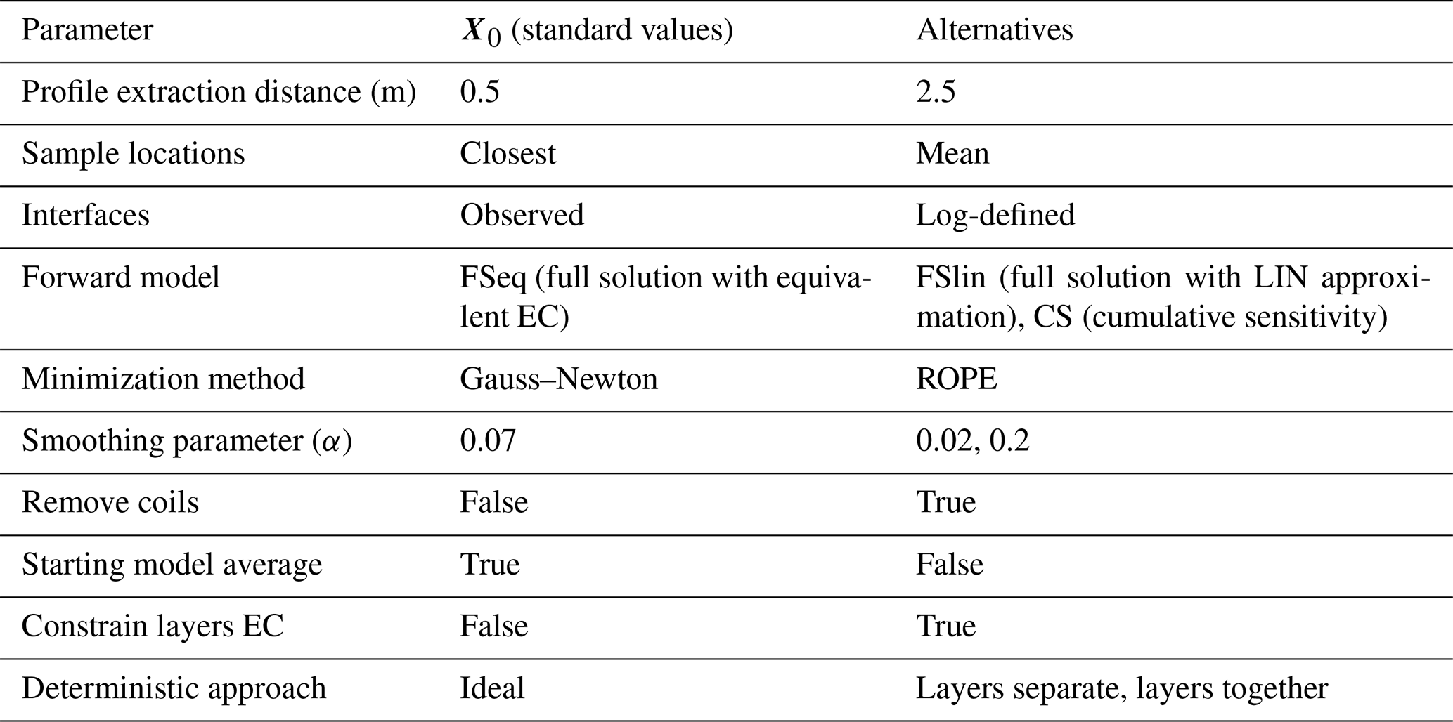
In this study, we defined the origin (X₀; see Table 1) as the standard set of parameters used for the whole data process (F) that correspond to a standard inversion and subsequent solution (Y₀), which is the standard solution for volumetric water content (θ₀):

$$\begin{array}{}\text{(3)}& F\left(\text{observed}\text{data},{\mathit{X}}_{\mathrm{0}}\right)={\mathit{Y}}_{\mathrm{0}}={\mathit{\theta }}_{\mathrm{0}}.\end{array}$$

Table 1 List of model parameters used across all the data workflows. Standard values for each parameter are presented in the second column (X₀) and alternatives to these values in the third column.

3 Results and discussion

3.1 Comparing EC data

A comparison of EC data obtained by the soil probe observations, standard FDEM inversion (using X₀ parameter values), and ideal EC for both sites is shown in Fig. 5 alongside the water and clay content of associated samples. The observed water content has mean values of 0.34 and 0.29 and variance of 0.003 and 0.008 for Site 1 and Site 2, respectively.

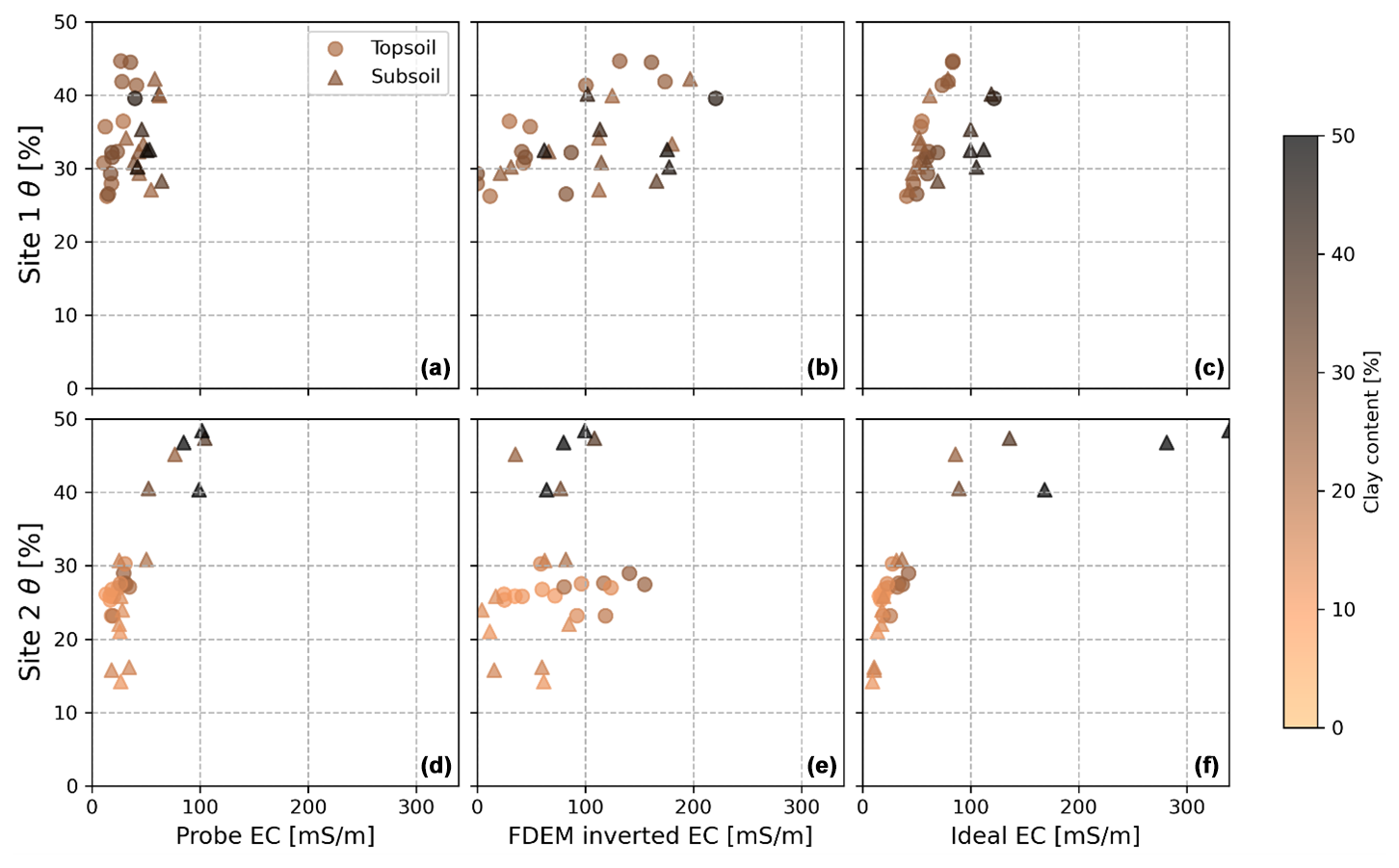
Figure 5 Comparison between EC obtained with the soil probe (a, d), FDEM standard inversion (b, e), and ideal EC (c, f) versus water content and clay content as an additional dimension. All the EC data are corrected for electromagnetic frequency and temperature (direct current EC at 25 °C).

Considering the EC measured by the soil probe as the reference for actual data, the inverted EC significantly deviates from this reality. Furthermore, while the ideal EC and soil probe EC display a similar trend, this trend is noticeably stretched (compare first and third column in Fig. 5). It is also noteworthy that as the difference between ideal and soil probe EC (for both sites) increases, so does the clay content, with a Pearson correlation of 0.83 (p<0.005), not shown in Fig. 5. This disparity becomes even more pronounced for clay contents exceeding ∼30 %, which is in accordance with the validity range of Eq. (2) (clay contents up to 33 %).

Figure 6 Bar plots showing median results of empirical modeling of soil properties. The median R² values are obtained after testing such models in test datasets randomly generated as 30 % of the original dataset and iterating 100 times to ensure good data distribution.

3.2 Empirical modeling results

The performance of empirical models for predicting observed soil properties is presented in Fig. 6. Poor predictions (negative median R² over test datasets) were obtained when considering topsoil and subsoil data jointly (LT) for model development over training datasets (i.e., not considering sample depth). This may be due to an oversimplistic modeling that does not consider sample depths. Negative R² values occur when the model fits the data worse than a simple horizontal line at the mean of the observed values. Approaches LS and LS2, which use different fitted functions per soil layer, resulted in better results as expected. No significant differences were observed in R² values for features EC_a uncalibrated and calibrated LIN or rEC_a. This may be due to the linear relationship between uncalibrated and calibrated EC_a and quasi-linear relationship with calibrated rEC_a, which does not add information to such variables as polynomial features (Lavoué et al., 2010). However, the FDEM-inverted EC data generally underperformed compared to the rest of features, with the only exception of the LS2 approach for θ prediction at Site 1, with a R²=0.19 and a RMSE = 0.047, while for Site 2 the maximum R² is 0.31, with a RMSE = 0.066.

Comparing performances for predicting different soil properties, EC_w was shown to be an easier target than any other soil property. EC_w prediction was generally better for Site 2 that does not have the influence of saline groundwater. Predicting CEC, clay content, and ρ_b, on the other hand, seemed to be highly site dependent.

An important consideration when interpreting the empirical approach is the disparity in scale between the soil volumes measured by FDEM (m³) and the smaller volumes analyzed in the laboratory (100 cm³). While some studies have addressed this issue, their conclusions are often site specific and inconsistent (see, e.g., Cong-Thi et al., 2024; Dimech et al., 2023). Despite these discrepancies, it is worth noting that non-inverted EC generally outperforms inverted EC for soil properties prediction, even though inverted EC represents a smaller soil volume (cubic decimeters). This performance gap may be attributed to errors in the EC inversion process rather than the difference in spatial scales.

When the best-performing models for θ prediction are implemented using the entire dataset (Fig. 7) – using both training and test data – this outperforms the modeling presented in Fig. 6, where only test data are incorporated into error assessment. While this is a common approach, we want to highlight this is improper practice to critically evaluate model performance as the inclusion of training data in error estimation results in an overestimation of model performance (Altdorff et al., 2017; Lipinski et al., 2008; Tibshirani et al., 2001). In other words, implemented model errors should not be confused with actual expected accuracy of target property predictions.

To evaluate the influence of other soil properties in θ prediction, the residuals of the implemented empirical models were correlated with other soil properties, but these were not significant.

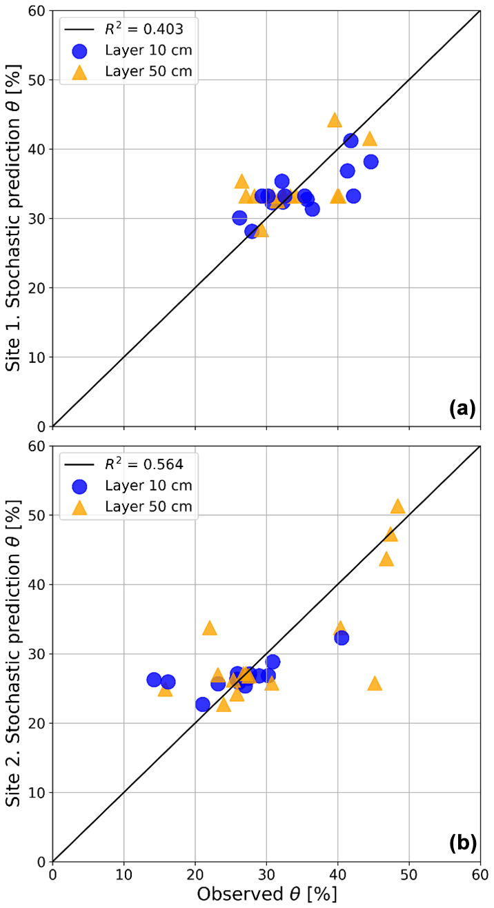
Figure 7 Empirical model implementation. Best-performant empirical models for θ prediction (based on Fig. 6 results) were implemented using the 30 samples per site. Panel (a) shows the data for Site 1, and panel (b) shows data for Site 2.

3.3 Sensitivity analysis

The result of the sensitivity analysis is presented in Fig. 8 for Site 1 (upper subplot) and 2 (lower subplot). Generally, no possible combination of parameter values yielded an RMSE lower than 11 % (or 0.11 cm³ cm⁻³) for θ predictions, which corresponds to a negative R² value; that is, they performed worse than a single mean solution. Additionally, the predictions for θ were worse for Site 2 than for Site 1, presumably due to the larger variance in θ data at Site 2. The standard solution θ₀ obtained using the X₀ parameter values was poorly performant too (see red lines in both subplots of Fig. 8). From Fig. 8, the boxes which differ the most from the rest represent the most sensitive parameters. For both sites, the most sensitive parameters are the minimization method used and the pedophysical model approach.

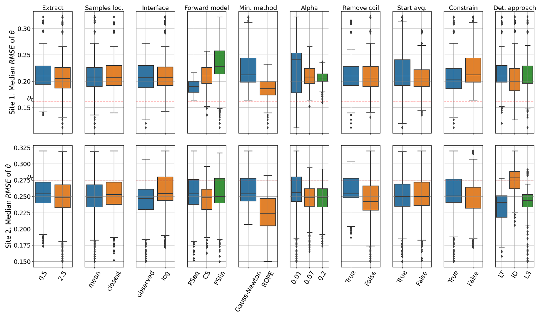
Figure 8 Box-and-whisker plot results of uncertainty analysis. The figure shows the error outcomes of an elementary effect sensitivity analysis using parameters involved in processing all FDEM data. The top row displays results for Site 1 and the bottom row for Site 2. The plotted data are the median of RMSE. The error associated with the θ₀ solution is highlighted in red. Each box represents 50 % of the data (i.e., the error associated with a specific parameter value), with a horizontal line indicating the median, while the whiskers represent 25 % of the data at each end.

Using the minimization method ROPE leads in general to better θ predictions, despite its average inversion error (R²=0.64 for Site 1 and R²=0.19 for Site 2) being higher than for Gauss–Newton (R²=0.75 for Site 1 and R²=0.94 for Site 2). Also, about 75 % of ROPE inversions for both sites did not converge or reached a negative R² error, while for Gauss–Newton most of the inversions converged with a positive R².

The optimal approach in deterministic modeling is not the same at both sites. While the ID approach was the best at Site 1, the best at Site 2 was LT. This could be because ID uses actual soil properties to populate the pedophysical model (focusing on variance of the error), and the LT approach uses average soil properties (attacking the bias error), resulting in an unclear benefit because of the general poor performance.

4 Limitations

Although the presented research focuses on comparing different choices made along modeling steps, it is important to highlight its site-specific nature (Boaga, 2017). Therefore, because both sites were selected based on their heterogeneous nature, the challenge that they represent is not necessarily representative of most common fields where the FDEM technique is applied, where collected EC FDEM data normally have a narrower range (Minsley et al., 2012; van der Kruk et al., 2018). Furthermore, the effects of scale disparities among soil sampling, ERT, FDEM, and probe measurements were not examined, even though they can introduce additional uncertainties when interpreting subsurface properties.

While several modeling parameters were tested, the data acquisition strategy remained unchanged. New insights might be gained by, for instance, using a different algorithm to select sampling locations (Brus, 2019) or reducing the FDEM crossline sampling density to better match FDEM data with ERT data at sampling locations. The FDEM data calibration strategy used in this study was indeed unique, and it assumes that the inverted ERT data accurately represent the subsurface. This assumption poses a limitation, as inverted ERT data can, in practice, contain acquisition and inversion errors, which ultimately impact FDEM data calibration (Minsley et al., 2012). Additionally, the evaluation of different parameters in the sensitivity analysis was not exhaustive, with its results being relative to the parameters chosen.

For instance, using different optimization methods would improve the FDEM inversion error and offer more flexibility in the inversion, such as allowing variable layer thicknesses. However, not all optimization methods, such as the Gauss–Newton method, support variability in subsoil layer depths. Additionally, only 1D forward and inversion models using FDEM methods were employed, without considering lateral smoothing through 2D or 3D inversions.

Furthermore, three different deterministic modeling approaches were tested using Eq. (2), but other pedophysical models were not considered. The difficulty in obtaining the EC_s parameter of Eq. (2) led to its exclusion, which might have compromised the model's effectiveness.

Lastly, the study was limited to univariable empirical modeling. Multivariable regression incorporating more than one feature (such as using inverted EC and uncalibrated EC), as well as other machine learning methods, was not explored.

5 Conclusions and suggestions

Absolute soil property quantification using the FDEM method in heterogeneous fields is far from being accurate and methodologically solved.

The classical field-specific empirical modeling of soil properties, though limited, still offers the most straightforward solution. Based on our cases, uncalibrated EC_a data can be used without compromising the effectiveness of such an approach. This bypasses the issues of physics-driven deterministic modeling, such as data calibration, robust EC estimation, geophysical inversion, and pedophysical modeling. Such empirical models should consider vertical soil variability; otherwise large mispredictions are expected. However, this is at the cost of building a dataset by sampling and analyzing the soil target properties at the desired exploration depth. In samples not used for training, water content predictions achieved a poor best estimation with an R² value of 0.31 (RMSE = 6.6 %), which may be inadequate depending on the application, whereas EC_w was better estimated. Scale disparity between FDEM field measurements and soil samples is a less significant issue than using inverted EC data for empirical estimation of soil properties. In the case that sampling is not an option, a universal deterministic approach can be followed at the expense of FDEM calibration data, e.g., through ERT. A comprehensive sensitivity analysis of this approach shows that no possible combination of modeling parameters could currently lead to reasonable predictions of water content for the studied sites. Particularly, the pedophysical model of Eq. (2) should be reworked and validated for soil samples above 30 % of clay content, and a pedotransfer function for EC_s would help to ease its implementation. Additionally, the minimization method implemented in geophysical inversion turned out to be of key importance. Thus, further work is required to improve the deterministic modeling predictions.