A multiagent socio-hydrologic framework for integrated green infrastructures and water resource management at various spatial scales

Green infrastructures have been widely used to manage urban stormwater, especially in water-stressed regions. They also pose new challenges to urban and watershed water resources management. This paper focuses on the green-infrastructure-induced dynamics of water sharing in a watershed from three spatial scales. A multiagent socio-hydrologic model framework is developed to provide an optimization-simulation method for city-, inter-city- and watershed-scale, termed Integrated GIs and Water Resources Management (IGWM), that comprehensively considers the watershed circumstances, the urban water managers, and the watershed manager–urban water manager interactions. We apply the framework to conduct three simulating experiments in the Upper Mississippi River basin, USA. Four patterns in city-scale IGWM are classified, and two dynamics of cost and equity in inter-city- and watershed-scale IGWM are characterized through various sensitivity, scenario, and comparative analyses. The modeling results could advance our understanding of the role of green infrastructures and the impact of water policy in urban and watershed water resources management and assist water managers in making associated decisions.

1 Introduction

In recent decades, urban water scarcity worldwide caused by urbanization, population growth, and climate change has necessitated new approaches to increase water supply (McDonald et al., 2014; Schewe et al., 2014). Green infrastructures (GIs), which are decentralized nature-based measures for rainwater and stormwater capture and recharge, have prevailed in many countries, such as the USA, the UK, China, and Australia (Dietz, 2007; Coutts et al., 2013; Zhou, 2014; Li et al., 2017). GI systems, as demonstrated by many studies, are effective in increasing water availability and reducing urban flooding, which, to some extent, can supplement the centralized water services provided by grey infrastructure systems (Rozos et al., 2010; Jayasooriya and Ng, 2014). Therefore, an increasing number of cities are incorporating GIs into their urban water systems (Daigger and Crawford, 2007; Sapkota et al., 2014). However, the development of GIs in urban areas can transform socio-hydrologic dynamics within a watershed at various scales (see Fig. 1). At the city scale, the development of GIs, hydrologically, can increase urban water storage capacity (Askarizadeh et al., 2015), thus altering the urban water cycle (Meng, 2022). Socially, GIs provide alternative water sources that enhance water users' choices and reduce water use costs (Zhan and Chui, 2016), gradually changing their water use habits (Kallis, 2010) and shifting the original balance of water supply and demand. At the inter-city scale, the benefits of GIs can encourage an increase in the proportion of GI systems in each urban area. The cumulative effect of these systems on the urban water cycle can increase (Palla and Gnecco, 2015), leading to local socio-hydrologic changes in each urban area that gradually affect the distribution of water resources within the watershed. This occurs because multiple urban areas along a river share water resources within the watershed. At the watershed scale, the over-development of GIs driven by self-interest in each urban area can result in an uneven distribution of water resources across the watershed (Glendenning et al., 2012), potentially causing conflicts between urban areas. These conflicts necessitate watershed-level water policies from higher authorities for their mitigation. Therefore, the GI-driven socio-hydrologic dynamics at various scales pose a series of challenges to urban and watershed water management. These challenges are managed by multiple interactive decision-makers with individual goals at different authority levels: the urban water manager (UWM), who is responsible for managing and maintaining the urban water system cost-effectively, and the watershed manager (WM), who is responsible for ensuring equitable water resource distribution across the watershed through policy setting. To simulate these GI-driven socio-hydrologic dynamics at various scales and optimize the behavior of relevant decision-makers at different authority levels, it is essential to develop new water management frameworks. These frameworks should incorporate GI development, rainfall utilization, and water resources management. This approach, termed Integrated GIs and Water Resources Management (IGWM), should be applied at various scales.

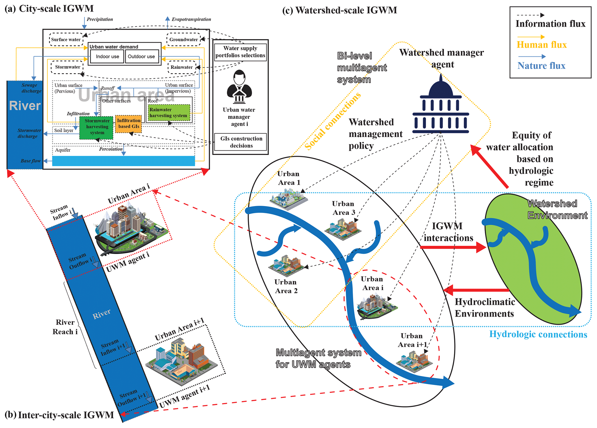
Figure 1 Schematic diagram of IGWM at three spatial scales. (a) At the city scale, UWMs must consider the simultaneous construction of GIs and water supply portfolios to meet urban water demands cost-effectively. (b) At the inter-city scale, IGWM decisions made in upstream areas can influence downstream areas due to hydrologic connections. (c) At the watershed scale, a WM needs to establish water policies that regulate UWM decision-making regarding IGWM, based on socio-hydrologic interactions. Note that UWM represents Urban Water Manager, GIs represents Green Infrastructures, IGWM represents Integrated GIs and Water Resources Management, and WM represents Watershed Manager.

A city-scale IGWM framework involves the integration of urban land use and water management strategies, specifically focusing on decisions related to GI construction and water supply portfolio choices. UWMs must plan the construction of diverse GIs with varying hydrologic performances within urban areas. These infrastructures should be designed to collect and store stormwater, thereby supplementing the urban water supply with stormwater resources. In general, GIs are divided into two groups depending on the desired flow regime: retention- and infiltration-based GIs (Fletcher et al., 2013). To be specific, the retention-based GIs, such as green roofs, cisterns, and rain barrels, can retain stormwater, which can be directly used for non-potable water uses or with filtration and disinfection for potable water uses (McArdle et al., 2011). Furthermore, the infiltration-based GIs, e.g., rain gardens, porous pavements, and wetlands, can restore some aspects of pre-development flow regimes in receiving water through the recharging of subsurface flows and groundwater, which can be indirectly used by groundwater abstraction (Endreny and Collins, 2009). Meanwhile, optimal water supply portfolios need to be determined from both grey infrastructure systems, such as rivers and aquifers (Sitzenfrei et al., 2013), and constructed GIs, including rainwater and stormwater harvesting systems, to meet various water demands (see Fig. 1a). The increased complexity introduced by GI development and the use of rainwater in the urban water system may render conventional urban water management approaches inadequate (Poustie et al., 2015) due to the involvement of more external socio-hydrologic factors in IGWM decision-making. For example, the magnitude and frequency of upstream inflow and precipitation directly influence the availability of surface water and stormwater for an urban area. Additionally, the socioeconomic development level of an urban area (e.g., residents' housing types and water use habits) can affect the selection of GI types, sizes, and locations (Chen et al., 2019). Therefore, it is crucial for a city-scale IGWM framework to address how to configure water resources drawn from grey infrastructure (i.e., surface water and groundwater) and from GIs (i.e., rainwater and stormwater), as well as developing relevant plans for GI construction. This approach aims to optimize the use of limited water supplies while minimizing costs.

At the inter-city scale, an IGWM framework must consider the cumulative effects of expanding GIs within urban areas. The increased rainwater storage capacity, enhanced groundwater recharge (Zhang and Chui, 2019), and elevated evapotranspiration (Ebrahimian et al., 2019) resulting from GI development can significantly alter the urban water cycle. Consequently, city-scale IGWM decisions made by UWMs can impact the broader hydrologic dynamics. In a watershed, multiple urban areas typically share water resources along a river, each striving to secure sufficient and affordable water for their maintenance and development needs. The modifications in the urban water cycle induced by city-scale IGWM decisions can alter the inflow and outflow patterns of an urban area. These regional hydrologic shifts can gradually propagate throughout the watershed due to the interconnected nature of the river network. Therefore, IGWM decisions made by an upstream UWM can influence those made by downstream UWMs, highlighting the interdependence of urban water management within a watershed. Some studies demonstrated that over-development of GIs might decrease the river flow to downstream areas (Glendenning et al., 2012), which may be detrimental to stream health (Fletcher et al., 2007). In comparison, others showed that expansion of GIs might, to some extent, decline the variability of river flow, which is beneficial to downstream water supply (Golden and Hoghooghi, 2018). Under the circumstances, all UWMs within a watershed make their own IGWM decisions rationally, not only depending on urban hydrologic states but also on anthropogenic activities from upstream urban areas (see Fig. 1b). Therefore, the interactive behavior among UWMs for IGWM forms a unique sequential multi-player interaction at the inter-city scale. This can be simulated by considering the hydrologic state of the first upstream urban area after implementing its own IGWM decisions, followed by the hydrologic state of the adjacent downstream urban area after its own IGWM decisions. These states transition sequentially along the river. This state transition process exhibits the Markov property (Frydenberg, 1990) – where the hydrologic state of an urban area depends only on the hydrologic state of the adjacent upstream area after making its IGWM decisions and the decisions of the urban area itself. Such interactions might lead to unexpected watershed-level performance. Therefore, it is essential for an inter-city-scale IGWM framework to investigate the socio-hydrologic dynamics of interactions among multiple urban areas in relation to their city-scale IGWM decisions.

In general, optimal decision-making for city-scale IGWM can reduce the cost of accessing water resources for individual urban areas. However, at the inter-city scale, uncoordinated IGWM efforts might lead to inequitable and unsustainable water resource distribution within a watershed (Müller et al., 2017), potentially causing conflicts between upstream and downstream urban areas. For a watershed-scale IGWM framework, a WM must implement policies, such as streamflow penalty strategies, to regulate the decision-making of UWMs and achieve equitable water distribution within the watershed. In this context, the WM and multiple UWMs form a bi-level system based on their respective authority levels, following hierarchical decision rules for the leader (WM) and the followers (UWMs). Specifically, the WM sets water policies at the watershed level, and the UWMs subsequently make their city-scale IGWM decisions with full knowledge of these policies. The WM can also adjust its policy prescriptions based on the rational responses of the UWMs (see Fig. 1c). In economic theory, this hierarchical interaction process is described as a Stackelberg game (Simaan and Cruz, 1973). Given that uncoordinated interactions among multiple UWMs for IGWM can result in inequitable water resource distribution within the entire watershed, a WM may face challenges when using traditional water policy approaches that generally overlook such interactions. Therefore, it is crucial for a watershed-scale IGWM framework to consider the impact of water policies on the socio-hydrologic dynamics of interactions among multiple urban areas.

Currently, there are rich studies related to city-scale IGWM, most of which focused on studying the following three critical aspects: (1) integrating water management framework with GIs, (2) assessing rainwater potential, and (3) modeling urban water cycle of a urban water system incorporating GIs. The first aspect involves building an integrated water management framework that combines conventional water supply systems with stormwater/rainwater harvesting schemes (Daigger, 2009). To determine the appropriate stormwater harvesting scheme option under different settings, Goonrey et al. (2009) developed a decision-making framework. To address on-site and catchment urban surface water issues, Ellis (2013) introduced sustainable drainage systems into a GI framework. Dandy et al. (2019) presented an integrated framework to help UWMs select and evaluate stormwater harvesting systems. The second aspect of the studies is mainly focused on the quantitative evaluation of rainwater/stormwater resources supply options in various urban areas. Kim et al. (2022) investigated the impact of water management strategies, such as rainwater harvesting, on urban water demand in Filton Airfield, UK, using water demand profiles and urban water cycle simulations. Kim et al. (2022) developed a framework to assess a variety of centralized and decentralized water supply options, including rainwater harvesting and groundwater extraction via private wells, for meeting urban water demand in southern India. Souto et al. (2022) studied the effects of a rainwater harvesting system in reducing the demand for drinking water in the city of Goiânia using two water balance models. Research addressing the third aspect has focused on developing models to simulate urban hydrologic regimes within a urban water system incorporating GIs, such as the Aquacycle (Mitchell et al., 2001), Urban Cycle (Hardy et al., 2005), City Water Balance (Last, 2011), UrbanBEATS (Bach et al., 2015), and SUWMBA (Moravej et al., 2021). These models, to some extent, allow users to improve their understanding of the impacts of various GIs options at different scales and to assess the comprehensive performance of the urban water systems across the entire urban water cycle. Although there is rich literature addressing issues of city-scale IGWM, there is very little work that comprehensively considers the selection of centralized and decentralized water supply options, as well as the decision-making associated with GI construction plans within a urban water system in changing environments. This has become a key issue of concern for UWMs. Therefore, more in-depth studies are needed to develop a decision-making framework that can assist authorities in making effective decisions about IGWM at a city scale.

In addition, several studies associated with inter-city-scale IGWM have attempted to investigate the issues of interactions between water users in a shared water resources system, especially in irrigation systems (Barreteau and Abrami, 2007; Berger et al., 2007). To better understand the effects of water users or managers' behaviors and their interactions in a watershed-scale water resource system, a diverse range of studies have utilized agent-based models to simulate the actions and interactions of autonomous water users or managers within a water resources environment (Bankes, 2002). These models are part of a broader computational framework known as multiagent systems, which consist of multiple interacting autonomous agents. The aim is to assess the collective effects of these interactions on the overall system (Barreteau and Abrami, 2007). Berglund (2015) reviewed an emerging area of research within water resources management that uses agent-based models and multiagent systems to simulate the water resources allocation and to predict the performance of infrastructure design. Giuliani and Castelletti (2013) explored the effect of different levels of cooperation and information exchange among water users on the upstream–downstream water conflict in a large-scale water resources system through using a well-designed multiagent system. Some studies have also focused on interactions between water users and the watershed environment, coupling multiagent systems with watershed hydrologic models (He, 2019; Du et al., 2020). Montalto et al. (2013) constructed an agent-based framework to analyze the effect of different spatiotemporal distributions of GIs determined by numerous household decision-makers on urban water cycle in South Philadelphia. Hung and Yang (2021) developed a reinforcement learning agent-based framework in which agricultural water users act as agents that learn and adjust their water demands based on interactions with the water systems. Similarly, Motlaghzadeh et al. (2023) employed a three-game model to construct a hierarchical multiagent decision-making framework for managing water and environmental resources under the uncertain conditions of climate change and complex agent characteristics. Additionally, Khorshidi et al. (2024) proposed an agent-based model framework to evaluate the suitability of transitioning to modernized surface irrigation systems from traditional practices. While these studies can inspire this study, there are some common limitations for modeling IGWM at an inter-city scale. Firstly, the studies of interactions between water users tend to focus on agricultural regions rather than urban regions and do not address the issues of interaction between urban areas driven by developing GIs and using rainwater sources within a watershed. Secondly, rule-based models have been widely used to simulate the behavior of water users or managers in a water resource system but are unable to describe the complex decision processes of city-scale IGWM due to over-simplified decision rules.

In the field of research within IGWM at a watershed scale, several studies have focused on the evaluation or design of water policies to manage interactions or conflicts among multiple water users within a watershed via using various multiagent systems (Berger and Ringler, 2002; Akhbari and Grigg, 2013; Lin et al., 2020). For instance, Kock (2008) developed and applied two agent-based models of society and hydrology to test relations between different water policies in a watershed and the level of water conflict in that watershed. Kanta and Zechman (2014) built a multiagent system framework by integrating a urban water demand and a supply model and considering water users and managers as agents. A wide set of water policies, such as conservation strategies and interbasin transfer strategies, set by the water managers, and the associated responses from the water users, were simulated via using the framework. Darbandsari et al. (2020) proposed a new conflict resolution model to assess different water management policies through simulating the interactions of all water users' behaviors. A Stackelberg-game-theory-based model was used to describe the leader–follower interactions between water users and managers within a basin. Although these previous studies can provide guidance for IGWM at a watershed scale in an exploratory way, there is still a gap in building a sound and flexible watershed policy framework for the design and evaluation of various water strategies to allocate limited water resources to urban areas that develop GIs and use rainwater resources, as well as for the simulation of the complicated responses of water supply and GI development in each urban area to these strategies.

This paper focuses on IGWM within a watershed composed of multiple urban areas that implement GIs and utilize rainwater at three spatial scales (see Fig. 1). At the city scale, we examine how an UWM can optimally configure various water resources extracted from rivers, aquifers, stormwater, and rainwater harvesting systems, alongside planning for GI construction, to maximize the efficient use of limited water supplies while minimizing costs. At the inter-city scale, we investigate the effects of interactions among multiple urban areas on the socio-hydrologic dynamics of the watershed, stemming from their city-scale IGWM decisions. At the watershed scale, we explore how a watershed water policy, such as a streamflow penalty strategy set by a WM, can influence the behaviors of all UWMs regarding city-scale IGWM and their interactions with each other. To address these issues, we develop a multiagent socio-hydrologic framework. Specifically, this framework includes (1) an agent-based model, developed by coupling an agent-based model for UWM with a hydrologic simulation model, to determine optimal decision-making for city-scale IGWM in changing watershed settings; (2) a multiagent system, created by integrating the aforementioned agent-based models with a streamflow routing model based on the Markov property, to simulate interactions in inter-city-scale IGWM and assess its impact on the entire watershed; and (3) a bi-level multiagent system, constructed by combining the multiagent system with an agent-based model for WM based on Stackelberg game theory, to mimic the interactions and feedback between a WM and multiple UWMs driven by the implementation of a watershed water policy in watershed-scale IGWM, ultimately designing an optimal watershed strategy. In addition, we also demonstrate our framework to conduct three numerical experiments based on a realistic basin – the Minneapolis–La Crosse section of the Upper Mississippi River, USA. The results obtained from these experiments allow us to characterize and classify the decision-making of city-scale IGWM for a UWM under different circumstances, to analyze the socio-hydrologic dynamics of the watershed induced by inter-city-scale IGWM, and to assess the role of a water policy in watershed-scale IGWM.

The outline of this paper is as follows: Sect. 2 introduces the multiagent model framework used to simulate city-scale IGWM decision-making by UWMs and the socio-hydrologic dynamics of inter-city- and watershed-scale IGWM, considering interactions both among UWMs and between UWMs and the WM. Section 3 details three simulation experiments based on the Upper Mississippi River basin to provide insights into IGWM at three spatial scales. Section 4 discusses and analyzes the results of the simulation experiments. It identifies optimal IGWM features for UWMs through sensitivity analysis and assesses interactions among multiple UWMs and the WM at inter-city and watershed scales using scenario and comparative analysis. Section 5 concludes the paper with a summary of findings, limitations, and proposals for future research.

2 Methodology

This section proposes a multiagent socio-hydrologic framework for solving the issues mentioned above of the IGWM at three spatial scales.

2.1 Overview of the multiagent system architecture

The framework considers UWMs and WMs within the watershed as individual agents. It includes (1) two agent-based models for urban water and watershed manager agents to realistically represent UWM and WM decision-making processes and (2) two hydrologic models – the Urban Water Balance Simulation Model (UWB-SM) and the Muskingum–Cunge routing model. The UWB-SM describes the dynamics of urban water balance induced by city-scale IGWM decisions, while the Muskingum–Cunge routing model simulates changes in streamflow in river reaches connecting adjacent urban areas. By integrating these components, we build an agent-based model and two multiagent systems to simulate GI-driven socio-hydrologic dynamics at three spatial scales for addressing IGWM issues (see Fig. 1). Specifically, the following is done:

1. An agent-based model combines the UWM agent-based model with the UWB-SM to address city-scale IGWM (see Fig. 1a).

2. A multiagent system integrates multiple UWM agent-based models with the Muskingum–Cunge routing models for inter-city-scale IGWM (see Fig. 1b).

3. A bi-level multiagent system combines the multiagent system with the WM agent-based model to simulate watershed-scale IGWM dynamics (see Fig. 1c).

Detailed introductions of the model components and structure are provided in the following sections.

2.1.1 Two agent-based models

Agent-based models for UWM. As illustrated in Fig. 1a, a UWM must simultaneously consider GI construction and water supply portfolios to meet diverse urban water demands cost-effectively. For GI construction, three types of GIs can be built to utilize rainfall resources within an urban area: infiltration-based GIs to enhance groundwater recharge by altering infiltration rates of pervious surfaces; rainwater harvesting systems to collect rainwater from roofs before it contacts the ground; and stormwater harvesting systems to collect stormwater draining off land areas, including roofs and ground surfaces (Fielding et al., 2015). The water supply portfolios involve four types of water sources classified by intake locations: surface water from nearby rivers, groundwater from aquifers beneath urban areas, rainwater collected via rainwater harvesting systems, and stormwater collected via stormwater harvesting systems (Steffen et al., 2013). Potable water demand is satisfied by surface water and groundwater supplies, whereas all water resources can support non-potable demands.

The agent-based model for UWM aims to determine cost-effective annual construction areas for the three types of GIs, considering urban land limitations, and determine least-cost monthly water supply portfolios to meet urban water demands, subject to allowable source amounts. The objective function is to minimize the annual IGWM cost, which includes the costs of GI construction, water supply, and wastewater drainage. Constraints include the available construction areas for GIs; monthly water supply limits for each water source; and monthly water demand requirements for potable water, total water, and urban irrigation for GI maintenance. Detailed descriptions of the UWM agent-based model are provided in Appendix B2.

Agent-based models for WM. As shown in Fig. 1c, the WM sets a water policy, specifically a streamflow penalty strategy, to regulate the IGWM decisions of all UWMs within a watershed. This strategy is inspired by water withdrawal regulations in regions like South Carolina (Nix and Rad, 2022), where over-extraction of surface water can incur penalties. The WM prescribes a series of low streamflow thresholds at checkpoints based on monthly hydrologic states; if the streamflow at an urban area's outlet falls below its threshold, a penalty fee is imposed on the respective UWM. This approach encourages UWMs to consider the externalities of their IGWM decisions, thereby adjusting their actions to account for potential costs (Baumol and Oates, 1988).

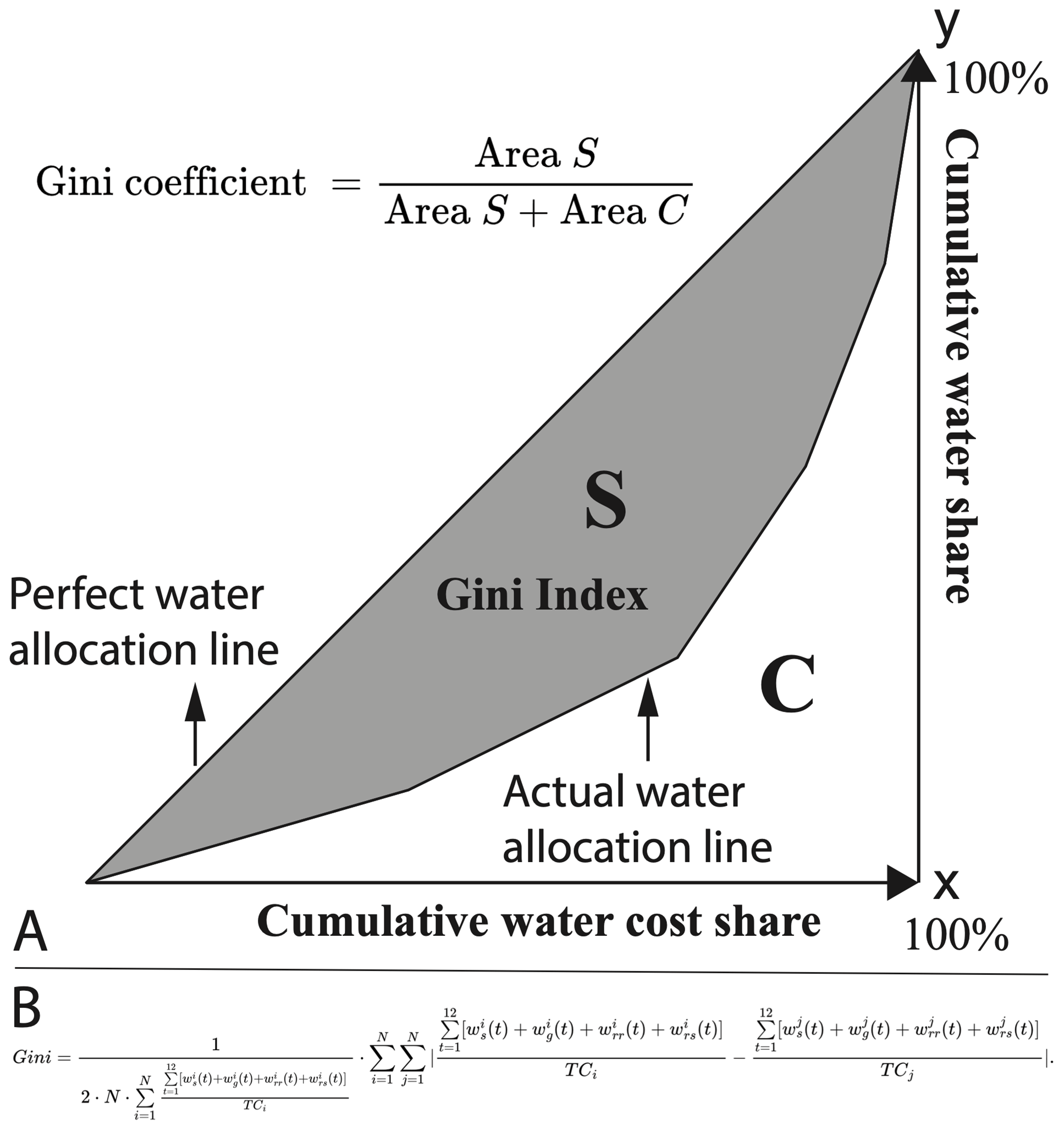
The WM agent-based model determines the monthly low streamflow thresholds at each checkpoint based on the hydrologic conditions of the corresponding river reach to influence UWM decisions effectively and achieve equitable water resource distribution in the watershed. The objective function aims to minimize the water allocation Gini coefficient, as proposed by Hu et al. (2016) and Xu et al. (2019), which measures equity in watershed-scale IGWM by calculating the equitable sharing of the used water quantity for each unit of cost (see Fig. 2). Minimizing the Gini coefficient ensures maximal fairness in water resource distribution. The model includes streamflow constraints that set the allowable range for low streamflow thresholds at each checkpoint. Detailed descriptions of the agent-based model for WM are provided in Appendix B3.

Figure 2 (a) Basic principle for calculating water allocation Gini coefficient and (b) the objective function for agent-based model for WM. Note that the relevant symbols in (b) are listed in Tables B1 and B2 in Appendix B1.

2.1.2 Two hydrological models

Urban water balance simulation model (UWB-SM). We developed a lumped urban water system model to describe the dynamics of urban water balance induced by city-scale IGWM decision-making. The model incorporates all urban water flows (natural and anthropogenic), grey urban water systems, and GI systems to simulate interactions between the water supply-wastewater discharge network, the rainfall-stormwater runoff network, and three types of GI systems within an urban area. Figure 3a illustrates the urban water mass balance modeled in the UWB-SM, showing water flow movements between seven storage units: roof, other surfaces, rainwater and stormwater harvesting systems, shallow soil layer, aquifer, and river. The UWB-SM receives input from rainfall and river inflow, which pass through both grey and green infrastructure systems, resulting in outputs in the form of evapotranspiration and river outflow. Water moves between the seven storage units, with the amounts of water in these units representing their states. These states are used to measure the total water balance within an urban area and to calculate available amounts of four water resources: surface water and groundwater extracted from the river and aquifer storage units and rainwater and stormwater collected by harvesting systems. Following Mitchell et al. (2001), indoor water use is divided into potable and non-potable demands, while outdoor water use is considered non-potable.

Figure 3 The structure of the UWB-SM. Note that relevant symbols in (b) and (c) are listed in Tables C1, C2, and C4 in Appendix C1.

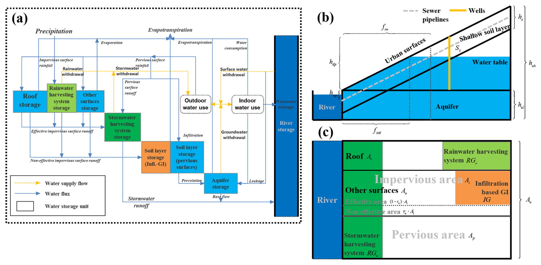
The vertical structure of the UWB-SM, illustrated in Fig. 3b, consists of four components: urban surfaces, shallow soil layer, aquifer, and river. The model simulates water flux transfers between these storage units based on the principle of water mass conservation, considering various surface-subsurface water interactions and pipe network exfiltration and infiltration. On urban surfaces, there are four water storage units: roof, other surfaces, rainwater, and stormwater harvesting systems (see Fig. 3c). The urban surface is divided into pervious and impervious areas based on infiltration rates. Impervious surfaces, where infiltration is negligible, are further divided into effective and non-effective areas. Effective areas directly drain runoff to the stormwater drainage system, while non-effective areas drain onto adjacent pervious areas, with remaining water evaporating. Pervious areas infiltrate part of the runoff into the underground soil layer, reducing runoff and enhancing groundwater recharge. Roofs and other surfaces, such as roads and paved areas, are classified based on the construction conditions of different GIs. Rainwater harvesting systems are assumed to be built only on roofs, while infiltration-based GIs (e.g., infiltration trenches and porous pavements) are constructed on non-roof impervious areas, turning them into pervious areas. Runoff generated from roofs, rainwater harvesting systems, and other impervious surfaces is managed through evaporation or rainwater extraction. Stormwater harvesting systems collect runoff from the entire urban surface for stormwater supply. The UWB-SM simplifies spatial features of the urban surface, focusing on the cumulative effects of three types of GIs on the urban water cycle and hydrological interactions.

The UWB-SM requires four types of input data: IGWM decision-making, urban water demand, hydroclimatic data, and urban land and water characteristics. Specifically, IGWM decision data update the monthly water supply amounts of four water resources and the annual construction areas for three GI systems as determined by a UWM agent. Urban water demand data include monthly indoor and outdoor water demands, which can be estimated based on the urban population and economic development levels. Hydroclimatic data comprise mean monthly river inflow, precipitation, and potential evapotranspiration within an urban area. Urban land and water characteristics are described by calibrated and measured parameters, which are listed in Table C2. Measured parameters relate directly to physical catchment characteristics and can be determined through measurement, observation, or local experience. The 12 calibration parameters, along with their units, symbols, and ranges, are grouped according to land features such as surfaces, soil layer, aquifer, river, and urban water system, as shown in Table C3. These values are adjusted during calibration to optimize the selected objective function. Detailed governing equations for the UWB-SM are provided in Appendix C2.

Muskingum–Cunge routing model. It simulates upstream–downstream hydrologic interactions between UWM agents in an associated river reach, as illustrated in Fig. 1b. For example, the upstream inflow for UWM agent i+1 in month t can be mathematically expressed as the outflow from UWM agent i in the same month and the next month (Garbrecht and Brunner, 1991; Weinmann and Laurenson, 1979). The Muskingum–Cunge routing model, which is used to simulate these interactions, is described in detail in Appendix C3.

2.2 Agent-based model for city-scale IGWM

Figure 1a illustrates the decision-making process of city-scale IGWM by an UWM agent and the resulting changes in urban water cycles. To simulate the UWM's behavior in city-scale IGWM, an agent-based model is developed by coupling the agent-based model for UWM with the UWB-SM. In this model, annual decisions on GI construction made by the UWM agent are first used as inputs to the UWB-SM. Subsequently, monthly water supply portfolio selections are represented by the UWM agent, while the resulting changes in urban water cycles are simulated in the UWB-SM. The agent-based model for UWM interacts with the UWB-SM through a coupling strategy. This coupling strategy enables us to use a simulation-based optimization approach to estimate and predict the UWM's decision-making in city-scale IGWM and the resulting urban hydrologic dynamics under different socioeconomic and hydroclimatic conditions.

The data exchange between the UWB-SM and the agent-based model for UWM occurs in two phases to ensure feasible solutions (Fig. D1b in Appendix D2). In Phase 1, an annual data exchange generates feasible GI construction decision variables for the UWM agent and initializes the UWB-SM. Initial data, including urban water demand, land and water characteristics, and hydroclimatic data, are input into both models. Annually available construction areas for infiltration-based GI, rainwater, and stormwater harvesting systems are determined by GI construction constraints and used to update the urban land features in the UWB-SM. In Phase 2, a monthly data exchange generates feasible water supply decision variables for the UWM agent. Each month, the UWB-SM runs at least twice, exchanging data with the agent-based model for UWM. The UWB-SM updates the urban hydrologic state based on the storage levels of seven storage units from the previous month and computes available runoff for stormwater harvesting. This information, along with the storage levels of four storage units (river, aquifer, rainwater, and stormwater harvesting systems) from the previous month, is used by the agent-based model for UWM to generate feasible monthly water supply decision variables. These variables are then transferred back to the UWB-SM to simulate urban hydrologic variables for the current month. The updated hydrologic variables are sent back to the agent-based model for UWM to verify the feasibility of the decision variables. If the decision variables fail the check, they are regenerated by the agent-based model for UWM. If they pass, the relevant IGWM cost is calculated, and the updated storage units' data are used to initialize the UWB-SM for the next month. This process continues until the termination criteria are satisfied, generating a feasible IGWM decision variable and associated annual cost.

The UWB-SM and the agent-based model for UWM are tightly coupled at the source code level, with subroutines of the agent-based model embedded into the UWB-SM. The primary data exchanged between the two models include water supply portfolios, GI construction plans, and hydrologic states. Given that some parameters of the agent-based model for UWM are computed by the UWB-SM, a corresponding solution approach is detailed in Appendix D2.

2.3 Multiagent system for inter-city-scale IGWM

Figure 1b illustrates the river connections between urban areas, which significantly affect the impact of GIs on urban and watershed hydrology in terms of water resource allocation. These river connections mean that all UWM agents must share surface water resources, and the decisions made by upstream agents can affect downstream agents (Glendenning et al., 2012). A multiagent system is constituted by considering multiple urban areas and interconnected river networks. In this system, all UWM agents are linked by a river network. Each UWM agent independently makes city-scale IGWM decisions – such as water supply portfolios and GI construction – based on its current hydrologic states and upstream inflow, which is influenced by the outflows from upstream areas and the decisions of associated UWM agents. The interactions among multiple UWM agents can be depicted as a sequence of city-scale IGWM decisions along river networks, as water is transported downstream. This interaction process exhibits the Markov property (Frydenberg, 1990), where the hydrologic state of a downstream urban area depends only on the hydrologic state of the adjacent upstream area after making its own IGWM decisions and its own decisions. This state transition process continues sequentially along the river.

The multiagent system for inter-city-scale IGWM is formulated by integrating the agent-based model for UWM (Eq. B1) with the UWB-SM and the Muskingum–Cunge routing model (Eq. C10), leveraging its Markov property. This system is modeled as a special type of multi-stage decision system (Bellman, 1966), where the sequence of decision-making for each UWM agent – city-scale IGWM – follows their spatial locations along river networks, from upstream to downstream. The hydrologic variable, specifically the upstream inflow for each UWM agent, is considered the state variable that describes interactions between agents. This can be expressed as follows:

$$\begin{array}{}\text{(1)}& \left\{\begin{array}{llr}\text{agent-based model for UWM }i+\text{UWB-SM},& \forall i& \left(\mathrm{01}\right)\\ \text{Muskingum–Cunge routing model}i\mathrm{in}t,& \forall i,t& \left(\mathrm{02}\right)\\ q_{\mathrm{ri}}^{\mathrm{1}}\left(t\right)=Q_t^{\mathrm{1}},\mathrm{and}{q}_{\mathrm{ri}}^i\left(\mathrm{0}\right)=Q_{\mathrm{0}}^i,& \forall i,t& \left(\mathrm{03}\right)\end{array}\right.,\end{array}$$

where the third row of Eq. (1) shows initial conditions for the multiagent system for UWMs, and $Q_t^{\mathrm{1}}$ and $Q_{\mathrm{0}}^i$ are the initial amounts of the upstream inflow for UWM agent 1 in month t and UWM agent i in month 0, respectively. The details of the multiagent system and the corresponding solution approach are presented in Appendix E1 and E2.

2.4 Bi-level multiagent system for watershed-scale IGWM

In the described multiagent system, each UWM agent minimizes its own IGWM costs without directly considering the external effects on other UWMs due to the Markov property of the system. This might lead to inequalities in water resource sharing, where upstream users might consume more surface water than downstream users, potentially increasing the IGWM costs for downstream areas (Giuliani and Castelletti, 2013). To address this inequality and promote sustainable water use in watershed-scale IGWM, a WM can implement policies such as a streamflow penalty strategy.

Under such policy interventions, each UWM agent must balance the costs of GI construction, water supply, and wastewater drainage with the potential penalty fees imposed by the WM for not meeting specified low streamflow thresholds. Consequently, the agent-based model for UWM is extended to include these penalty fees in the annual IGWM cost function. Details of this model extension are provided in Appendix F1.

As illustrated in Fig. 1c, a streamflow penalty strategy may prompt upstream UWM agents to adjust their IGWM decisions to increase outflow, thereby minimizing penalty fees and benefiting downstream agents. These adjustments can shift the interactions within the multiagent system, impacting water resource distribution within the watershed, which can be quantified using the water allocation Gini coefficient set by the WM. The WM can assess the policy's effects on the watershed by evaluating this metric and iteratively adjusting the policy to find the optimal solution. This process represents an interaction between the WM and UWMs in watershed-scale IGWM under a streamflow penalty strategy. This interaction is not solely determined by the WM or the UWMs; both parties aim to optimize their objectives (equity for the WM and cost minimization for UWMs) under respective constraints (streamflow for the WM and GI construction, water supply, and demand constraints for the UWMs) and the reactions of the other party. This decision-making process follows the Stackelberg game theory (Von Stackelberg, 2010), where the WM makes the initial decision, and UWMs respond to optimize their objectives with full knowledge of the WM's decision. The WM then optimizes its objective based on the rational reactions of the UWMs.

Leveraging the Stackelberg game framework (Dempe, 2002), we construct a bi-level multiagent system by combining the agent-based model for WM with the multiagent system comprising multiple extended agent-based models for UWMs and the relevant hydrologic models. This system can be formulated as follows:

$$\begin{array}{}\text{(2)}& \left\{\begin{array}{l}\text{agent-based model for WM};\\ \mathrm{where}{W}_i,{\mathrm{GI}}_i\mathrm{solves}\\ \left\{\begin{array}{ll}\text{extended agent-based model for UWM }i+\mathrm{UWB}-\mathrm{SM},& \forall i\\ \text{Muskingum–Cunge routing model}i\mathrm{in}t,& \forall i,t\\ q_{\mathrm{ri}}^{\mathrm{1}}\left(t\right)=Q_t^{\mathrm{1}},\mathrm{and}{q}_{\mathrm{ri}}^i\left(\mathrm{0}\right)=Q_{\mathrm{0}}^i.& \forall i,t\end{array}\right.\end{array}\right.,\end{array}$$

where $[-{]}_{*}$ represents the parameter being from the simulation calculation of the UWB-SM. W_i and GI_i represent the decision variables of water supply portfolios and GI construction for UWM agent i. The details of the bi-level multiagent system and the pertaining solution approach are illustrated in Appendix F2 and F3.

3 Case study and experimental design

In this section, the proposed multiagent socio-hydrologic framework is utilized in a case study on the Minneapolis–La Crosse section of the Upper Mississippi River, United States, and three numerical experiments are designed to characterize the decision-making of IGWM at three spatial scales.

3.1 Overview of the study area

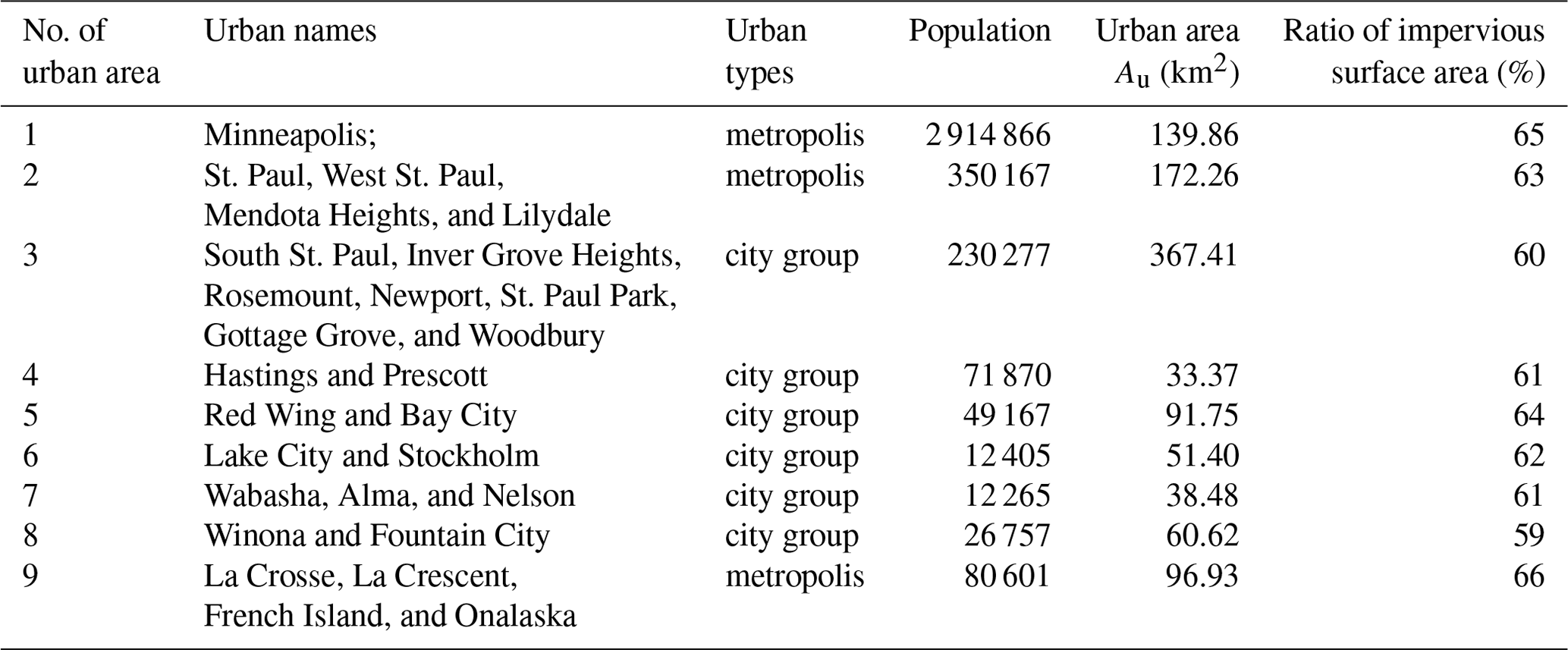
As Fig. 4 shows, the Upper Mississippi River basin ranges in latitude from 47 to 37° N, and it flows roughly 2092 km, from Lake Itasca (northern Minnesota) to the Ohio River (southern Illinois), which covers seven states of the USA, such as Illinois, Iowa, Minnesota, and Wisconsin, and has a watershed area of 489 508 km². The main river and its tributaries have an average annual discharge of 3576 m³ s⁻¹, which has three high-flow (late April, late June, and October) and two low-flow (midsummer and late winter) periods as a result of varied rain and snow conditions (Baldwin and Lall, 1999). In the watershed, more than 70 % of the area is used for agriculture and animal husbandry. Only 5 % of the site has been converted to urban areas. However, it has a population of about 24 million, especially in the metropolitan high-density regions (> 100 000 people km⁻²), such as Minneapolis–St. Paul, Minnesota, and La Crosse, Wisconsin. It is estimated that over 5.3×10⁶ m³ of water is withdrawn from the Upper Mississippi River each day in the 60 counties for municipal and public supplies.

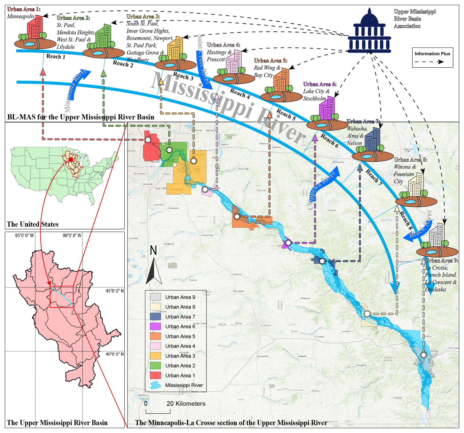
Figure 4 Schematic diagram of the study area. Notice that the base map and metropolis and city group maps in the bottom right of the figure are from Esri (2012) and U.S. Census Bureau (2018), respectively; the US boundary map and the Upper Mississippi River basin map in the bottom left of the figure are from U.S. Census Bureau (2018) and USGS (2021), respectively.

There are three primary reasons for selecting the Upper Mississippi River basin as the case study for conducting numerical experiments. First, although the widespread use of GIs for rainwater harvesting is not prevalent in the USA, the study (Ennenbach et al., 2018) has demonstrated the potential for rainwater harvesting in this watershed, attributed to its humid climate and abundant annual precipitation. However, this study also indicates that seasonal variations in water demand necessitate a deeper exploration of rainwater harvesting potential. Applying the socio-hydrologic framework to the basin can provide valuable insights into this potential. Second, despite being a water-rich basin, water sharing among the riparian urban areas remains a significant concern due to the high demands for environmental and agricultural purposes, strict water level regulations for navigation, and high-density urbanization. Climate change is expected to drastically alter the probability distribution of streamflow, increasing the frequency and magnitude of both high and low streamflow extremes. Consequently, even high-flow river basins also might face nonstationary drought risks (Dierauer and Zhu, 2020). A simulation study showed that climate change could result in streamflow decreases in all seasons except winter within the basin (Lu et al., 2010). Third, there are notable similarities between the actual case and the simulated case by the proposed model. For instance, in fact, the Upper Mississippi River Basin Association as WM aims to implement a water level management policy (Reed et al., 2020), which mirrors the multi-player management structure assumed in the proposed model. Additionally, surface water and groundwater are crucial sources of water widely used by urban areas, and green infrastructures are gradually encouraged and expanded to manage urban stormwater by local communities and authorities (Askew-Merwin, 2020; Guo, 2023).

In this study, the Minneapolis–La Crosse section – approximately 236 km long – of the Upper Mississippi River basin, a high-density urban area, is considered the study area (see Fig. 4). Note that the study only focuses on the urban water use and allocation, which perhaps is a small percentage of the basin water resource in the study region. Figure 4 indicates that there are nine main riparian urban areas along the section, i.e., i=1, 2, …, 9. Some are metropolises with a large population for these urban areas, such as Minneapolis, St. Paul, and La Crosse. The others are city groups that consist of multiple small cities, such as Red Wing and Bay City. In short, the basic features of urban areas in the study site are shown in Table 1.

Table 1 The basic features of urban areas in the study site.

3.2 Experimental design

Given the background of the study area, the all urban area – metropolises or city groups – is assumed as a UWM agent that makes city-scale IGWM decisions individually, which can be formulated by Eq. (B1), and the Upper Mississippi River Basin Association is regarded as the WM agent that regulates these urban areas, and the associated interactions among UWMs and between WM and UWMs are formulated by Eqs. (E1) and (2), respectively. In the case study, we address the above issues of IGWM at three spatial scales through observing and comparing the results of the decision making of WM and UWM agents and interactions in IGWM simulated by the proposed model under different socio-hydrologic settings. Therefore, three numerical experiments to IGWM at city, inter-city, and watershed scales are designed in the following:

3.2.1 Experiment 1 of IGWM at a city scale

The experiment aims to identify and classify the characteristics of optimal decision-making for city-scale IGWM by UWM agents under different hydroclimatic settings. Firstly, a sensitivity analysis of the agent-based model for city-scale IGWM (see Sect. 2.2) is performed. All urban areas within the studied region are considered study objects. The associated agent-based models for city-scale IGWM are run multiple times under different combinations of upstream inflow and precipitation, which are the model's input parameters, to calculate the associated optimal decision-making scenarios. The baseline values for these two hydroclimatic parameters are obtained from the USGS, and six scenarios are created by decreasing and increasing the baselines by 25 %, 50 %, and 75 %, respectively, covering high and low streamflow and rainfall extremes. Secondly, based on the optimal decision-making scenarios of city-scale IGWM under mixed hydroclimatic conditions, a k-means clustering method (Likas et al., 2003) is employed to classify all UWMs' decision-making strategies. This classification characterizes the patterns of city-scale IGWM in changing environments by summarizing the similarities in UWMs' decision behavior under specific hydroclimatic conditions.

3.2.2 Experiment 2 of IGWM at an inter-city scale

The experiment is designed to examine the impacts of inter-city-scale IGWM on the socio-hydrologic dynamics of the watershed and investigate how watershed hydroclimatic and socioeconomic conditions affect these interactions. For the first objective, two scenarios are simulated using the multiagent system for inter-city-scale IGWM (see Sect. 2.3). The first scenario, serving as the experimental group, includes GI construction decisions and the usage of rainwater and stormwater. The second scenario, serving as the control group, excludes GI development and rainwater and stormwater usage by setting the maximum available areas for constructing three types of GIs to zero in all agent-based models for UWM. By comparing the results of these two groups, we identify the potential impacts of inter-city-scale IGWM on water use cost, equity of water resource allocation, and available surface water distribution within the watershed, thereby quantifying the relative contribution of GIs to these impacts.

For the second objective, a sensitivity analysis of the experimental group is conducted. Various combinations of watershed settings (i.e., watershed upstream inflow, precipitation, and urban water demands) are considered. The scenario including GI development and rainwater and stormwater usage is set as the baseline. Similar to Experiment 1, monthly precipitation and watershed upstream inflow are proportionally varied from 25 % to 175 % of the baseline to simulate hydroclimatic dynamics. Additionally, monthly urban water demands, encompassing both indoor and outdoor demands, are adjusted from 25 % to 175 % of the baseline to represent socioeconomic changes in the watershed.

3.2.3 Experiment 3 of IGWM at a watershed scale

This experiment is designed to investigate the influence of a streamflow penalty strategy on the socio-hydrologic dynamics of the watershed within the context of IGWM and to examine the impacts of different hydroclimatic and institutional conditions on the interactions of watershed-scale IGWM. For the first objective, a policy simulation of the bi-level multiagent system for watershed-scale IGWM (see Sect. 2.4) is conducted. The optimal solution of this bi-level system can be defined as Stackelberg equilibrium points (Dempe, 2002) – equilibria between the WM and UWMs in watershed-scale IGWM where no party has an incentive to alter their decisions. Multiple equilibrium points are likely in such a system (Dempe, 2002); hence, all equilibria need to be identified and analyzed to assess the possible effects of the streamflow penalty strategy. The baseline penalty rate is specified as USD 0.005 per cubic meter. This rate is artificial due to the absence of an existing penalty strategy in the study area. The baseline rate is determined by referencing an actual water withdrawal regulation in South Carolina, USA (Nix and Rad, 2022), and through comprehensive parameter analysis (Parsapour-Moghaddam et al., 2015; Rosegrant et al., 2000) to ensure it can affect all UWMs' decision-making in the study area. By comparing the results with those from Experiment 2, we evaluate the potential impacts of the streamflow penalty strategy on water use cost, equity of water resource allocation, and surface water distribution within the watershed.

For the second objective, a sensitivity analysis is conducted under varying conditions of the penalty rate, watershed upstream inflow, and precipitation. The aforementioned policy simulation scenario is set as the baseline. Monthly precipitation and watershed upstream inflow are proportionally varied from 50 % to 150 % of the baseline to simulate hydroclimatic dynamics. Six penalty rates – USD 0.002 per cubic meter, USD 0.004 per cubic meter, USD 0.005 per cubic meter (baseline), USD 0.006 per cubic meter, USD 0.008 per cubic meter, and USD 0.010 per cubic meter – are set to represent different institutional conditions. In cases with multiple equilibria in the bi-level multiagent system, we only consider the equilibrium with the lowest mean cost per unit of water as the corresponding result for watershed-scale IGWM.

3.3 Data collection and processing

In the proposed framework to the case study, some parameters of the two agent-based models and two hydrological models need to be determined by collecting, processing, and estimating actual data from diverse sources.

For the parameters of UWB-SM, as detailed in Table C1 of Appendix B, the urban water demand data (36×9) were derived from urban populations and layouts using the method of Last (2011). The hydroclimatic data inputs (27×9) were estimated using raw data on streamflow, precipitation, and temperature from the USGS Current Water Data for the Nation (https://waterdata.usgs.gov/nwis/rt, last access: 1 May 2021) and the Global Historical Climatology Network daily (GHCNd) databases (https://www.ncei.noaa.gov/). Specifically, upstream inflow data were identified from GIS maps of urban areas and estimated using the map correlation method (Archfield and Vogel, 2010) with monthly streamflow observations from USGS stations because of the location difference between the urban area's inlet and the associated USGS stations. Evaporation and evapotranspiration data were calculated using the method of Ravazzani et al. (2012) with temperature data from the GHCNd database. The urban area data (1×9) were sourced from the U.S. Census Bureau (http://www.census.gov/, last access: 12 June 2021), and urban land features (4×9) were derived from remote sensing images (Last, 2011), as shown in Table C2 of Appendix B. Urban-depth-related data were obtained using various methods: mean aquifer depths at low topographic points (1×9) were assumed to be 10 m plus riverbed depths from the National Elevation Dataset (NED; https://datagateway.nrcs.usda.gov/, last access: 25 June 2021), while aquifer depths at high points (1×9) were calculated using linear fitting to urban hypsometric curves (Sharma et al., 2013). These assumptions are believed to have minimal impact due to the region’s abundant water supply. Mean well depths for groundwater withdrawal (1×9) were averaged from nearby wells in the USGS Groundwater Data for the Nation database (https://waterdata.usgs.gov/nwis/gw, last access: 4 July 2021). Maximum ratios for constructed areas of rainwater, stormwater harvesting systems, and infiltration-based green infrastructure (3×9) were set at 50 % to test maximum urban rainfall utilization potential, though actual ratios may be lower. Mean depths for shallow soil layers (1×9) and wastewater pipe networks (1×9) were set at 3 and 2 m, respectively, based on similar settings (Frost et al., 2016). Mean effective porosity (1×9) was estimated at 10 % from the report by Prior et al. (1953). Storage capacity data (4×9) were determined based on urban layouts using the method of Frost et al. (2016).

For the parameters of the agent-based model for UWM, as shown in Table B2 in Appendix C, the construction cost data for three types of green infrastructure (GIs) (3×9) were estimated based on the EPA cost databases (https://www.epa.gov/, last access: 23 July 2021) following the method of Houle et al. (2013). The associated cost scaling coefficients (3×9) were derived using a non-linear fitting method (Marquardt, 1963). Cost-related parameters for surface water and groundwater supply (4×9) were set according to the recommendations by Kirshen et al. (2004), while those for stormwater and rainwater harvesting (2×9) followed the recommendations of Dallman et al. (2016). Parameters for sewage drainage costs (2×9) were set based on Guo et al. (2014). Due to a lack of specific data for each urban area, these cost parameters were uniformly applied. Water-availability-related parameters (24×9) were determined by setting the minimum storage levels for surface water withdrawals based on the minimum monthly historical streamflow from the USGS datasets using the above same method. Minimum storage levels for groundwater withdrawals were set based on the mean depths of wells. Water-supply-capacity-related parameters (2×9) were set equal to the corresponding maximum monthly indoor water demand. The ratio of soil moisture for plant demand (1×9) was uniformly set at 0.31 based on Mitchell et al. (2001) recommendations. Additionally, for the parameters of agent-based model for WM, as shown in Table B3 in Appendix C, minimum and maximum historical streamflow data (24×9) were obtained from the USGS datasets using the above same method.

3.4 Model setup

In the framework, the other parameters of the UWB-SM and the Muskingum–Cunge routing model were evaluated through model calibration and validation using estimated historical streamflow data via the above same method.

For the calibration parameters of UWB-SM, as detailed in Table C3 in Appendix C, these were obtained by calibrating and validating the UWB-SM against estimated historical monthly outflow data derived from USGS datasets. The calibration process utilized estimated monthly inflow from USGS databases and monthly rainfall data from NOAA databases as inputs for the UWB-SM. During calibration, rainwater and stormwater supplies were excluded, and urban water demands (both indoor and outdoor) were assumed to be met solely through surface water and groundwater supplies, with a set ratio of 1:1. Monthly surface water and groundwater supply amounts were determined based on this setting. The simulated monthly outflow data from the UWB-SM were then compared with the estimated outflow data for calibration and validation. Detailed calibration and validation results are presented in Table 2.

(Kling et al., 2012)

Table 2 Details and representative results of calibration and validation for two hydrologic models. ^* represents the representative results for the two hydrologic models for urban area 1. KGE, NSE, R and B represent four types of performance metrics – the Kling–Gupta efficiency (Kling et al., 2012), the Nash–Sutcliffe coefficient of efficiency (Nash and Sutcliffe, 1970), the correlation coefficient between simulated and observed streamflow, and the percent bias (Gupta et al., 1999), respectively.

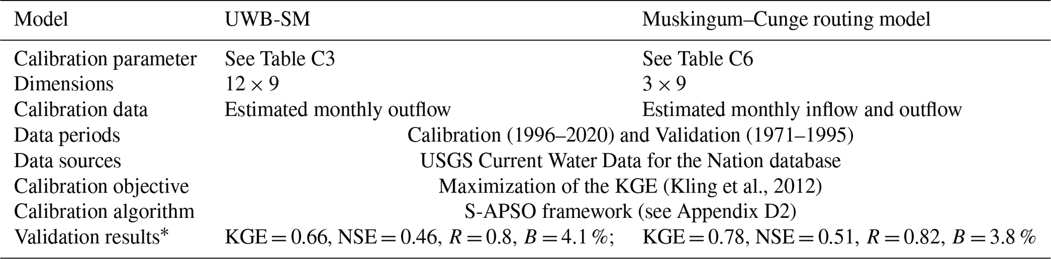
For the calibration parameters of the Muskingum–Cunge routing model, as shown in Table C6 in Appendix C, these were obtained by calibrating and validating the model using estimated historical monthly outflow data from the upstream urban area and inflow data for the adjacent downstream urban area. Detailed calibration and validation results for the Muskingum–Cunge routing model are also provided in Table 2.

4 Results and discussion

The results of these experiments and the associated analysis are discussed as follows.

4.1 Characteristics of city-scale IGWM in changing environments

The classified results of UWMs' decisions of IGWM to different environments are illustrated in Fig. 5a. As Fig. 5a shows, there are four IGWM patterns for UWMs in response to the different combinations of upstream inflow and rainfall inputs. The region of light-blue dots is defined as pattern 1, which represents the similar reactions of UWMs in the decision-making of IGWM to the high upstream inflow and rainfall inputs. The region of green dots indicates pattern 2, indicating the consistent behavior of IGWM for UWMs to the low upstream inflow and high precipitation settings. Similarly, patterns 3 and 4 are set in the region of dark-blue and yellow dots, which denotes the analogous decision-making of IGWM for UWMs in the study site under high (low) inflow and low (low) rainfall conditions respectively. The result indicates the homogeneous behavior of city-scale IGWM for all UWMs in the relatively extreme hydroclimatic conditions in the study region.

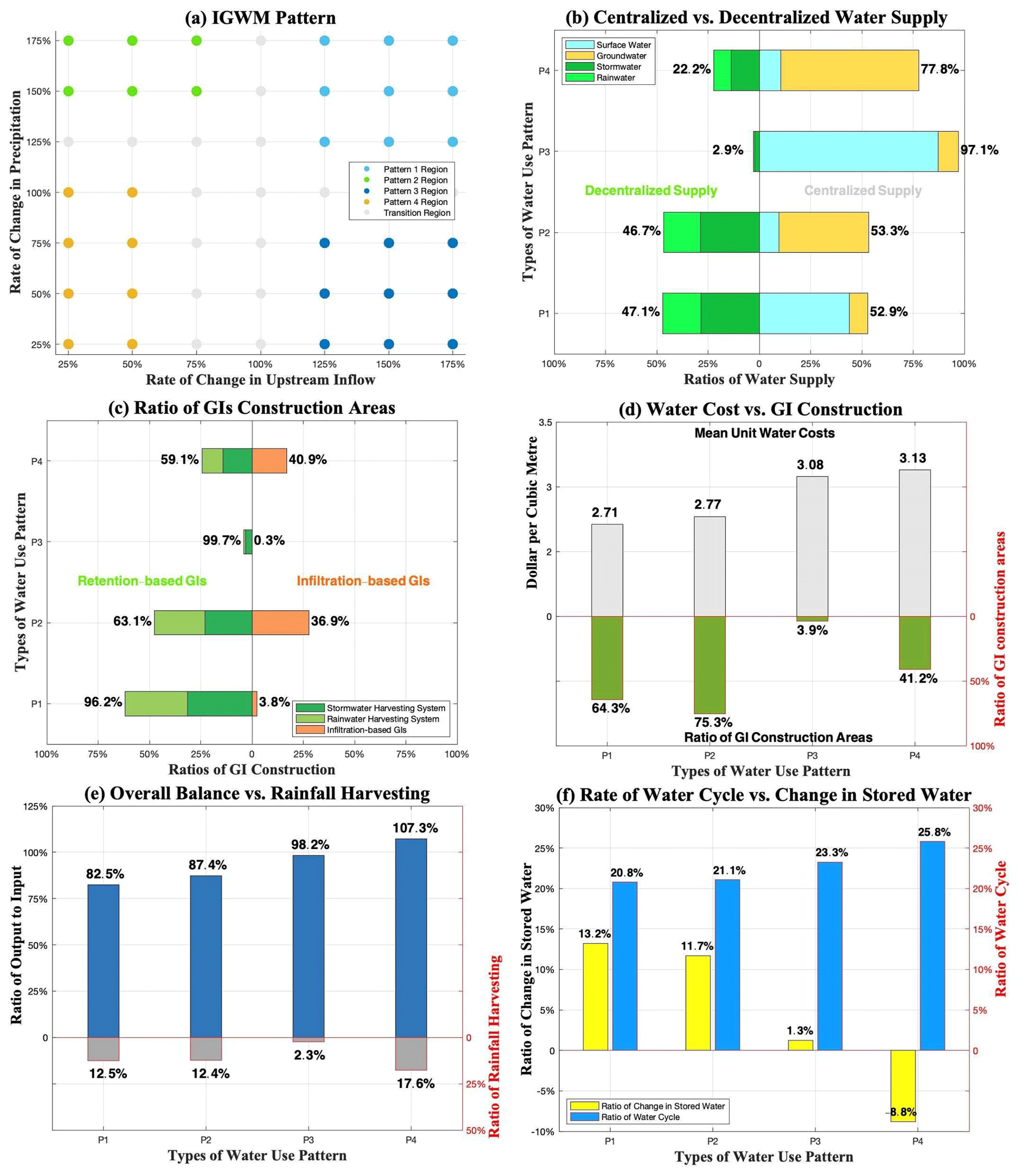
Figure 5 The classified results of city-scale IGWM in different environments. (a) Four IGWM patterns can be classified based on four color dots. (b–d) Different ratios of water supply portfolios and GI construction and the costs of water use are shown in the four patterns. (e–f) Four patterns significantly influence the urban water cycle. Note that in (e), the Ratio of system water output to input measures urban water balance, calculated as the sum of monthly evapotranspiration, consumption, and outflow (output) divided by the sum of monthly upstream inflow and rainfall (input). The Ratio of rainfall harvesting is the ratio of combined stormwater and rainwater supply to total rainfall. In (f), the Ratio of water cycle is the annual ratio of total water supply (surface water, groundwater, stormwater, and rainwater) to total urban stored water (sum of monthly storage across seven units: roof, other surfaces, rainwater, stormwater, soil layer, aquifer, and river). The Ratio of change in stored water is the difference between stored water in the last and first months, divided by stored water in the first month.

The characteristics of the four IGWM patterns mentioned above are shown in Fig. 5b–f. The ratios of water supply portfolios and GI construction in the four patterns are illustrated in Fig. 5b–d. There are large distinctions in the IGWM between the four patterns; in pattern 1, centralized and decentralized water account for 52.9 % and 47.1 % of total water supply, respectively, which means that stormwater and rainwater are widely utilized. More than 80.0 % of centralized water supply is from surface water. In the aspects of GI construction, over three-fifths of available urban areas is used to develop stormwater and rainwater harvesting systems, which accounts for 96.2 % of total GI construction areas. These results show the responses of IGWM to the high upstream inflow and rainfall inputs – UWMs prefer to use stormwater and rainwater directly to meet urban non-potable water demand by stormwater and rainwater harvesting systems for the sake of cost and to supply surface water to meet potable water demand. In pattern 2, similar to pattern 1, stormwater and rainwater are also heavily used directly to satisfy non-potable demand. At the same time, groundwater is the main potable water resource due to the low upstream inflow input. Accordingly, over 75 % of available areas is utilized for GI development, 35.9 % of which, unlike pattern 1, is for infiltration-based GIs for groundwater recharge. In pattern 3, stormwater and rainwater are hardly used (only 2.9 % of total water supply), and the construction of the associated GIs (only 3.9 % of available urban areas) is also limited due to the scarcity of precipitation. The surface water resource is dominant in urban water supply, accounting for 87.2 % of total water withdrawals because of the high upstream flow inputs. In comparison, stormwater and rainwater are partially used (22.2 % of total water supply) directly or indirectly by constructing GIs at a moderate level (41.2 % of available urban areas) in pattern 4. This might be because UWMs have to collect and use all kinds of available water resources as much as possible when system water inputs – rainfall and upstream inflow – are low. Hence, the groundwater is supplied more extensively for maintaining water supply steadily. It is worth mentioning that infiltration-based GIs, which account for 16 % of total GI construction areas, are, to a great extent, built to enhance aquifer recharge for reducing the costs of groundwater abstraction. In addition, Fig. 5d also illustrates the mean IGWM costs per unit of water in the four patterns. Undoubtedly, the costs of the pattern under high system water input conditions are lower than those under low water inputs.

Figure 5e and d illustrate the four indexes used to measure urban water cycle defined by Kenway et al. (2011) under these patterns, which show that the impacts of the four IGWM patterns on the urban water cycle. As Fig. 5e shows, the ratios of system water output to input and rainfall harvesting vary from pattern to pattern. Except pattern 4, the ratio of system water output to input of the rest of the patterns is smaller than 1, which means that the relevant IGWM patterns can increase water storage in an urban system, especially the pattern 1 and 2 with relatively large areas of GIs – 17.5 % and 12.6 % of water inputs are stored, respectively, which, to some extent, decreases the outflow of the urban catchment. The result is consistent with the Glendenning et al. (2012) results. However, in contrast to the other patterns, the ratio of system water output to input of the pattern 4 indicates the decreases in urban water storage. In this circumstance, to build a small range of infiltration-based GIs (i.e., the ratio of rainfall harvesting = 17.6 %) to increase groundwater recharge is limited. In addition, as shown in Fig. 5f, the ratios of water cycle increase in order from pattern 1 to 4, and the associated ratios of change in stored water have an opposite trend. These results also are consistent with the above results in Fig. 5e.

Our simulation study demonstrates the reasonable responses of UWM agents to different hydroclimatic settings in city-scale IGWM. Specifically, the hydroclimatic environment determines the availability of the four types of water sources, thereby influencing UWMs' selection of IGWM patterns from an economic perspective. Furthermore, the IGWM patterns chosen by UWMs can alter the urban water cycle, which, in turn, affects the hydrologic environment of the watershed.

4.2 Characteristics of inter-city-scale IGWM in changing environments

The results of the inter-city-scale IGWM in the two cases are shown in Table 3. The ratios of water supply portfolios of the all urban area in the two scenarios are shown in the 2nd–5th and 9th–10th rows of Table 3. In the case without GIs – a control group – surface water use fractions gradually decrease from the upstream to the downstream areas. For example, the ratios of surface water in urban areas 1, 5, and 9 are 0.85, 0.79, and 0.73, respectively. It might be because of a trend that the available amounts of surface water gradually decrease along with the river (see the blue line in Fig. 6a). These results indicate the adverse impacts of upstream water users on the downstream water users in surface water withdrawals. That is, water extraction from a stream in the upstream areas reduces the available amounts of surface water in the downstream regions, which would increase the costs of surface water withdrawal for the downstream urban areas, thereby forcing them to substitute other water resources, such as groundwater. In contrast, in the case with GIs – an experiment group – the fractions of surface water use appear to be independent of the study area locations due to stormwater and rainwater use via GIs. However, it might aggravate the adverse impacts, i.e., upstream–downstream imbalance of available surface water. For example, the ratios of surface water use markedly decrease in the downstream urban areas, especially in urban areas 6, 8, and 9, which have adopted IGWM pattern 4 – the high ratio of groundwater use. This may be because the upstream UWMs prefer to use stormwater and rainwater resources through developing GIs, such as IGWM pattern 1 and 2, to minimize the costs of water use (Cooley et al., 2019). However, as mentioned before, IGWM pattern 1 and 2 can reduce the outflow of the urban subcatchment (see Fig. 5e), which might worsen the decrease in available surface water in the downstream region (see the red line in Fig. 6a). In addition, the 8th and 12th rows of Table 3 also show the Gini coefficients (Eq. B4a) in the two scenarios – 0.0129 and 0.0169, indicating that the GI construction to use stormwater and rainwater intensifies the imbalance in water use in the study area.

Table 3 Results of the inter-city-scale IGWM in the two scenarios.

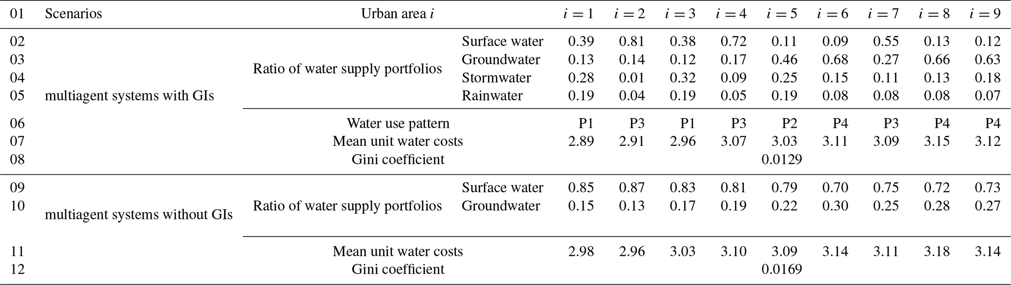
Note that the Ratio of water supply portfolios for urban area i is calculated as follows: the amounts of a type of water source supply divided by the total amounts of water supply in the urban area i. Mean unit water costs for urban area i is obtained as follows: the total IGWM costs divided by the total amounts of water supply in the urban area i.

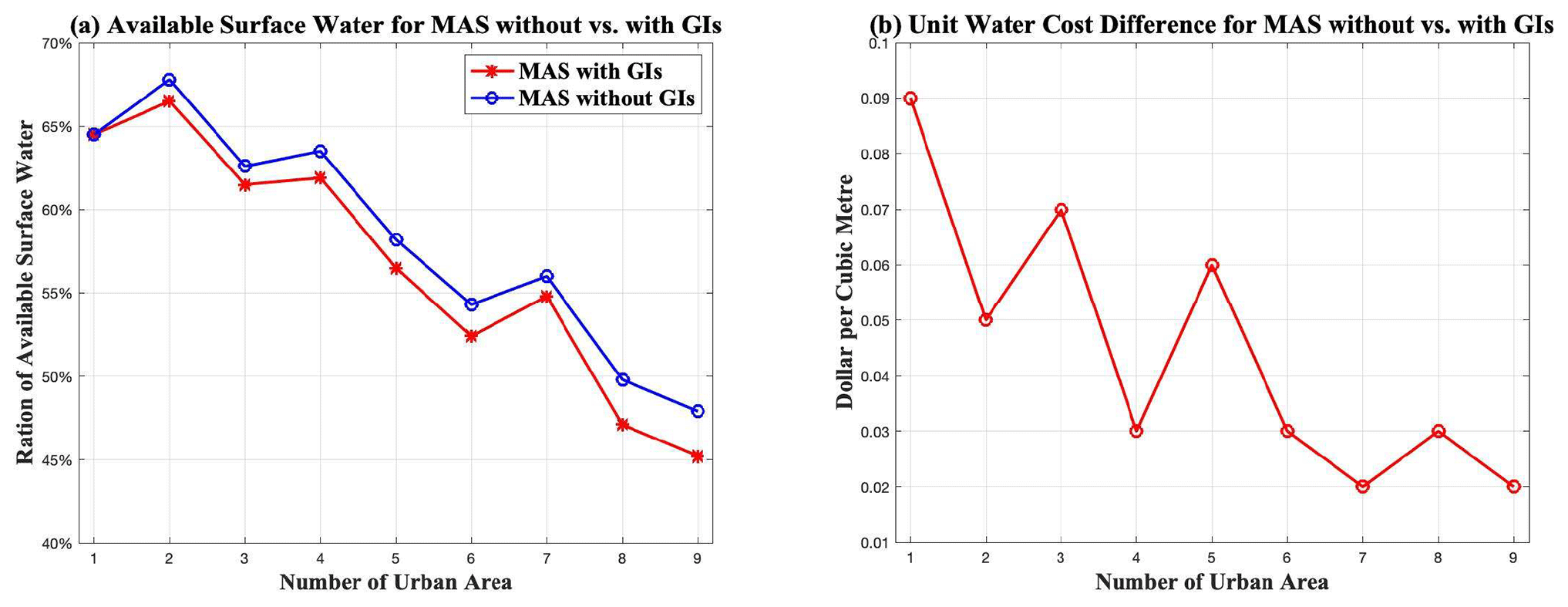
Figure 6 Available surface water and unit water cost difference in the two scenarios. (a) There is a trend that the available amounts of surface water gradually decrease along with the river, and GI development might worsen the trend. (b) There is a trend that costs between the two scenarios continuously decrease along with river. Note that in (a), Ratio of available surface water for urban area is set as the average of the ratio of the available monthly storage levels of river for water withdraw to the maximum theoretical that levels in an urban area. In (b), Unit water cost difference for urban area is calculated as follows: the difference of the mean unit IGWM costs in the urban area in the scenarios of the multiagent systems without and with GIs.

The 7th and 11th rows of Table 3 illustrate the IGWM cost per unit of water for each urban area in the two scenarios. There is a trend that the unit water costs constantly increase from the upstream to the downstream region, indicating the adverse impacts of the upstream–downstream imbalance of the surface water on the cost of water use for the downstream urban areas. In comparison, the costs of water use in the multiagent systems with GIs are smaller than those without no GIs for the all urban area. In contrast, the differences in these costs between the two scenarios continuously decrease from urban area 1 to 9 (see the red line in Fig. 6b). The reasons behind these results might be that there are two main factors – upstream inflow and GIs – affecting the costs of water use in the multiagent system for UWMs, especially for the downstream UWM agents. In general, the upstream inflow reduction can decrease the amounts of surface water, thereby increasing the cost of water use for the downstream UWMs. Conversely, rainwater and stormwater use via GIs can increase the available amounts of water resources and decrease water supply costs. In the multiagent system for UWMs, especially for the downstream UWM agents, the cumulative effect of the upstream IGWM decision behavior on streamflow gradually amplifies along the river. In contrast, the impact of the GIs on rainfall resource use generally remains stable due to the limitations of climatic, physical, and socioeconomic conditions. Therefore, the combination of the two effects might lead to a gradual decrease in the impact of GIs on the cost of water use along with the river.

Our findings reveal a persistent upstream–downstream imbalance in water resource access, exemplified by stark contrasts in surface water reliance between urban areas – from 85 % in upstream regions (e.g., urban area 1) to 73 % in downstream zones (e.g., urban area 9) in without GI scenarios. This disparity reflects systemic inequities: downstream areas face heightened costs due to diminished surface water availability, causing reliance on costlier groundwater sources. Crucially, GI adoption intensifies these tensions – while reducing city-scale costs (e.g., via stormwater harvesting in pattern 1), it inadvertently reduces downstream inflows by 12 %–18 % (Fig. 6a), amplifying inter-urban conflicts akin to a “tragedy of the commons” (Hardin, 2018). These results underscore the dual-edged impact of GIs: though locally cost-effective, watershed-scale implementation risks entrenching inequities by privileging upstream urban areas. To reconcile this tension, policies must integrate negotiated water-sharing agreements that harmonize localized GI benefits with watershed-wide equity, ensuring sustainable and equitable resource allocation across urban boundaries.

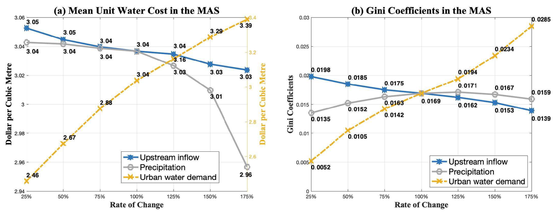
Figure 7 Changes in unit water costs and Gini coefficients under different social and hydroclimatic settings. (a) These is a non-linear inverse relationship between the cost of water use and the system water inputs. (b) There is an inverted U-shaped curve for the Gini coefficient when the precipitation increases. Note that in (a), Mean unit water costs in the multiagent system is obtained as follows: the total IGWM cost divided by the total amounts of water supply in the multiagent system.

The mean unit costs and the Gini coefficients in the multiagent system for UWMs under different precipitation, upstream inflow, and urban water demand inputs are illustrated in Fig. 7a and b, which show the influences of different social and hydroclimatic settings on the socio-hydrologic dynamics of the watershed in the context of inter-city-scale IGWM. In Fig. 7a, the blue and grey lines represent the changes in the mean costs per unit of water use in the all urban area under different precipitation and upstream inflow inputs. It shows a non-linear inverse relationship between the cost of water use and the system water inputs – the mean cost of water use in a watershed-scale IGWM decreases with the increases in both watershed upstream inflow and rainfall. Notice that the cost of water use in the multiagent system for UWMs is more sensitive to the precipitation than upstream inflow. Notably, the mean cost of water use decreases from USD 3.01 per cubic meter to USD 2.96 per cubic meter when the rainfall increases from 150 % to 175 %. It appears that rainfall inputs, when they go beyond a certain threshold, might have a profound effect on the IGWM cost of the multiagent system for UWMs. This might be due to the fact that more and more UWMs can switch IGWM patterns from pattern 3 or pattern 4 to pattern 1 or pattern 2, with the available rainfall exceeding a given threshold, leading to a significant decline in water use costs. These results are consistent with the results in Fig. 5d. In comparison, as the yellow line in Fig. 7a shows, the cost of water use in the all urban area is highly sensitive to the urban water demands. The increases in urban water demands are equivalent to the decreases in available water resources within an urban area, which greatly adds to the costs of water use.

Figure 7b shows the changes in the equity level of water use in the all urban area under different hydroclimatic and socioeconomic settings. The blue and grey lines in Fig. 7b represent the trends of Gini coefficients under mixed precipitation and upstream inflow conditions – it tends to proportionally decrease as the upstream inflow increases, while there is an inverted U-shaped curve for the Gini coefficient when the precipitation increases; it reached a peak (0.0171) when the ratio of the rainfall to the baseline is equal to 125 %. On the side of the upstream inflow, these results show that the reduction in watershed upstream inflow harms the equity levels of water use in watershed-scale IGWM. The possible reason is that the Markov property of the multiagent system for UWMs has a cumulative effect on the reduction in surface water availability along with the river. It can, to some extent, amplify the surface water conflicts between the upstream–downstream urban areas as the watershed upstream inflow decreases. On the side of the precipitation, the impact of rainfall on the equity of water resources distributions among urban areas is more complicated. The reasons for the increase in the Gini coefficient as the precipitation increase slightly might be that the water use costs for the upstream UWMs decrease remarkably by substituting stormwater and rainwater for surface and groundwater water as the rainfall increases. In contrast, in the downstream regions, the reduction in the relevant costs is limited because the cumulative effect of upstream inflow mentioned above limits the intention of the corresponding UWMs to switch IGWM patterns to use more rainfall resources economically. However, as the precipitation increases significantly, the abundant rainfall encourages the downstream UWMs to use stormwater and rainwater via GIs cost-effectively, reducing water use costs sharply, thereby making the watershed-scale IGWM more equitable. In comparison, the Gini coefficient in the all urban area is more sensitive to upstream inflow than rainfall. This is because the cumulative effect of upstream inflow might offset the impact of rainfall due to the Markov property of the multiagent system for UWMs.

Our findings demonstrate that inter-city-scale IGWM is shaped by dynamic interactions between hydrologic conditions and social drivers. Hydrologically, rainfall variability exerts a stronger influence on water use costs due to the cost-effectiveness of stormwater and rainwater resources, while shifts in upstream inflow disproportionately affect equity in water distribution – a consequence of the Markov property, where UWMs optimize decisions based on immediate inputs without accounting for downstream cascading effects (e.g., reduced surface water availability in downstream areas, as shown in Fig. 6a). Socially, rising urban water demands amplify both cost and equity challenges, as seen in fragmented governance structures that prioritize localized GI benefits (e.g., upstream adoption of pattern 1) over watershed-scale resilience, forcing downstream agents into costly groundwater-dependent strategies (pattern 4). These systemic flaws underscore the urgency of institutional reforms. For instance, interactive data platforms, akin to those in water-rights trading markets (Tu et al., 2015), could bridge communication gaps between urban water managers by providing real-time hydrologic and economic metrics. Such tools would enable adaptive adjustments to GI investments and withdrawal limits, aligning localized actions with watershed-wide equity goals – a critical need under climate change, where shifting streamflow distributions threaten to exacerbate existing imbalances.

4.3 Impacts of water policy on watershed-scale IGWM

The results of the policy simulation to the bi-level multiagent system are shown in Table 4. As Table 4 shows, there are two Stackelberg equilibrium situations in the bi-level multiagent system, which means the two possible designs of the streamflow penalty strategies for the WM agent can achieve the minimum equity objective in the study region. An illustration of the water supply portfolios and the relevant water use patterns in the all urban area under the two equilibrium situations is in the 2rd–6th and 10th–14th rows of Table 4. A spatial homogeneity in the UWMs' responses to the water policy can be observed based on the associated ratios of water supply portfolios. For example, whether it is equilibrium 1 or 2, most UWM agents prefer to adopt a similar IGWM pattern, such as pattern 3 in equilibrium 1 and pattern 2 and 4 in equilibrium 2, in contrast to the case without the water policy (see the 6th row of Table 3). This might be because the streamflow penalty strategy has a similar effect on altering the IGWM cost of the all urban area in the study watershed, forcing some UWMs to change their water supply portfolio selections to a specific IGWM pattern to increase outflows of urban systems for avoiding high penalty fees. These findings can also be supported by the curves of the fractions of available surface water in each urban area (see in Fig. 8a). As Fig. 8a illustrates, the available amounts of surface water withdrawal for each urban area in the two equilibriums (i.e., the blue and green lines) are larger than in the scenario without the water strategy (i.e., the red line).

Table 4 Results of watershed-scale IGWM in the bi-level multiagent system.

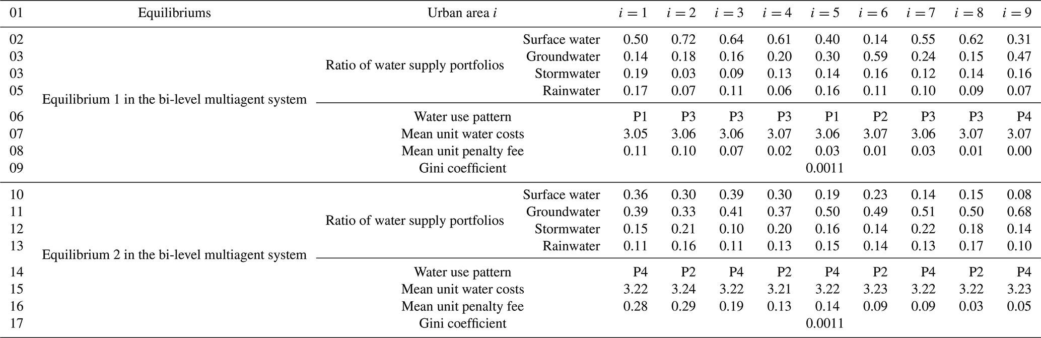
Note that the Mean unit penalty fee for urban area i is obtained as follows: the penalty fees divided by the total amounts of water supply in the urban area i.

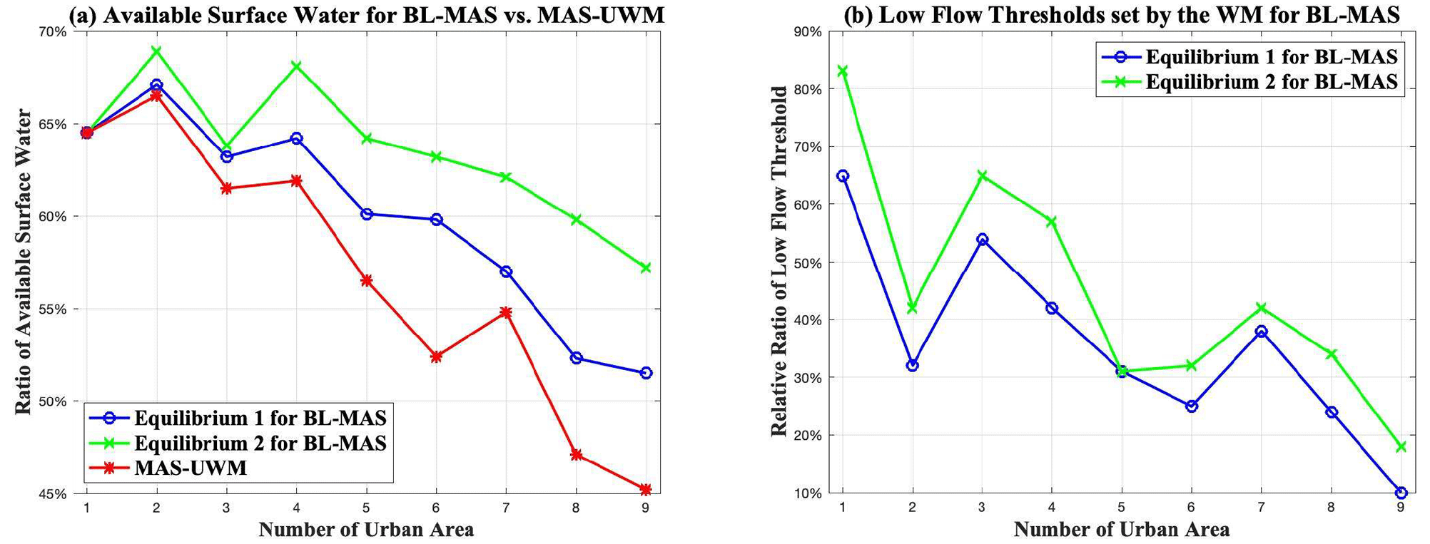
Figure 8 Available surface water and low-flow threshold in the bi-level multiagent system. Note that in (b), Relative ratio of low-flow threshold for urban area calculated as follows; The average of the ratio of the monthly low-flow threshold set by WM agent to the maximum theoretical that threshold in an urban area.

The costs and equity levels in the study area are shown in the 7th–9th and 15th–17th rows of Table 4. In the aspects of cost, to compare with the no policy case (see the 7th row of Table 3), the mean costs per unit of water use of the study area in the two equilibriums (USD 3.06 per cubic meter and USD 3.22 per cubic meter) are higher than the cost in the no policy case (USD 3.04 per cubic meter). This is because some urban areas pay penalty fees, such as urban areas 1 and 2, and others switch IGWM patterns, such as urban area 3, which increases the water use cost. These results demonstrate the reactions of the UWMs to the water strategy set by the WM in IGWM at a watershed scale; the intervention of the water policy to the multiagent system for UWMs can force UWM agents to make a trade-off between the penalty fee and the IGWM cost in a city-scale IGWM. In the aspects of equity, undoubtedly, the Gini coefficients in the two equilibriums (0.0011) are the same, which are lower than in the no policy case (0.0169; see the 8th rows of Table 3). It means that the two policy designs can mitigate the inequity of water sharing in the study region to some extent.

The 6th and 14th rows in Table 3 show that different effects of two streamflow penalty strategies on the decision making of UWM agents for city-scale IGWM. That is, most UWM agents prefer to select the IGWM pattern 3 – to withdraw more surface water – in equilibrium 1. In contrast, the UWM agents in equilibrium 2 are inclined to choose pattern 4, i.e., to extract more groundwater, which is easy to increase the outflows of urban subcatchment (see Fig. 5e) to avoid the penalty fees. These results are consistent with the curves of the fraction of available surface water (see the blue and green lines in Fig. 8a). The available amounts of surface water in the study area in equilibrium 2 are higher than that in equilibrium 1. Economically, the IGWM costs and the penalty fees per unit of water use in equilibrium 2 are greater than those in equilibrium 1. These results can be explained in part by the curves of the relative ratio of low-flow thresholds in the two equilibriums (see Fig. 8b); the low-flow thresholds in equilibrium 2 (i.e., the green line) are higher than those in equilibrium 1 (i.e., the blue line), which means that the policy in equilibrium 2 is more stringent than that in equilibrium 1. As a result, the UWMs in equilibrium 2 have to further change IGWM patterns – over the withdrawal of groundwater and reduction in rainfall capture – to increase the outflow of the urban subcatchments to avoid the harsh penalty policy. It may cause over-reactions of the UWM agents in IGWM to the watershed water policy, thereby leading to the unnecessary costs of water use as well as the unreasonable water supply portfolios in the watershed. Therefore, the policy design in equilibrium 1 is regarded as a good watershed policy, but equilibrium 2 is not in the study area.

Our findings demonstrate that the efficacy of penalty-driven policies hinges on reconciling the priorities of watershed-scale managers (WM agents) and city-scale managers (UWM agents). The Stackelberg framework captures inherent power asymmetries between these actors – where WM agents enforce equity through penalties, while UWM agents prioritize local cost optimization – a dynamic that risks policy failure. For instance, stringent penalty rates in equilibrium 2 (Fig. 8) trigger irrational overreactions, such as excessive groundwater extraction (Table 4), destabilizing aquifer sustainability and inflating regional water costs. This mismatch underscores the limitations of siloed governance: WM agents lack granular insight into local trade-offs, while UWM agents neglect downstream equity.

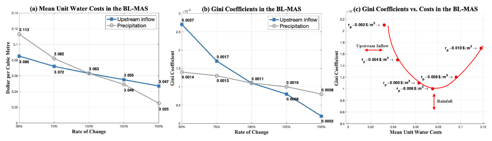
Figure 9 Changes in unit water costs and Gini coefficients under different institutional and hydroclimatic settings.

Figure 9a and b illustrate the mean unit water costs and the Gini coefficients of the study area under different upstream inflow and precipitation conditions, respectively. As Fig. 9a and b show, both the costs of water use and the Gini coefficients of the study area decrease as the upstream inflow and the precipitation increase. This might be because the increases in the upstream inflow and the precipitation not only enable the UWM agents to have more choices to make IGWM decisions to reduce the costs of water use but also mitigate the water conflicts among urban areas in the study site, encouraging the WM agent to loosen the water penalty policy. In addition, the cost of water use is more sensitive to the rainfall, while the Gini coefficient, in contrast, is easily affected by the alteration in upstream inflow, which ties in with the results in Fig. 7a and b.

The water use costs and the Gini coefficients of the equilibrium situations in the bi-level multiagent system under different penalty rates settings are illustrated in Fig. 9c. As Fig. 9c shows, the costs of water use of the study area increase as the penalty rate increases, as expected. To avoid over-high penalty fees, the UWM agents have to alter the IGWM pattern further to increase the outflows of urban systems, thereby increasing water use costs. However, there is a U-shaped curve for the Gini coefficients when the penalty rate increases; the Gini coefficient reaches a nadir (0.001) when the penalty rate is r_p= USD 0.006 per cubic meter. The possible reasons for these results are that the impact of the water strategy is too weak to affect UWMs' decision behavior of IGWM as the penalty rate is too low, whereas an overly high penalty rate might force UWMs to make unreasonable IGWM decisions, both of which fail to mitigate water conflicts between urban areas. Therefore, a suitable penalty rate is crucial in achieving equity in watershed-scale IGWM under a specific socio-hydrologic environment. For example, in the study, the reasonable penalty rate is set as USD 0.006 per cubic meter in comparison with other alternative penalty rates.

Our results demonstrate that streamflow penalty strategies, while effective in enhancing equity impose a dual-edged impact, increase water costs for upstream areas but might fail to fully address systemic disparities for downstream communities. For instance, the Gini coefficient’s heightened sensitivity to upstream inflow (Fig. 9b) reveals that marginalized downstream regions disproportionately bear the costs of water use, even under penalty strategies. These findings also highlight the critical role of penalty rates within streamflow penalty strategies. A well-calibrated rate can simultaneously reduce water use costs and enhance equity in water allocation, whereas a poorly designed rate exacerbates imbalances – heightening risks of policy failure. To mitigate such risks, adaptive management principles, such as iterative penalty adjustments informed by stakeholder feedback (Gonzales et al., 2019), could align incentives across governance levels. By embedding real-time hydrological data and equity metrics (e.g., Gini coefficients) into penalty frameworks, these strategies would address power asymmetries inherent in the Stackelberg hierarchy, ensuring policies not only regulate upstream UWM decisions to promote equitable allocation but also minimize costs across urban areas, even under climate-change-induced hydrological uncertainties.

4.4 Concluding remarks

To summarize the results and findings, we can draw the following concluding remarks:

• The cost-effectiveness of developing GIs to use rainwater in urban areas is highly dependent on the hydroclimatic conditions of the watershed.

• On a city scale, the development of GIs to use rainwater can reduce the cost of water use. However, on a watershed scale, it may exacerbate the inequity of water sharing among urban areas due to the Markov property of the multiagent system in inter-city-scale IGWM.

• The streamflow penalty strategy set by WM to mitigate inequity in water sharing among urban areas is effective under suitable penalty rate settings. However, due to the bi-level multiagent system property in watershed-scale IGWM (i.e., Stackelberg game), there is a risk of policy failure.

• An adaptive management framework is critical to prioritize vulnerable downstream stakeholders via iterative penalty rate adjustments and interactive data platforms, redirecting cost savings to reduce upstream–downstream IGWM disparities and promote sustainable water equity.

• The proposed framework is flexible and can be adapted to other basins with different socio-hydrologic settings by adjusting parameters and model settings for various model components. For example, different water policies, such as water trading schemes, can be simulated within this framework by improving the agent-based model for WM.

5 Conclusions, limitations and future research

This study addresses three critical issues of IGWM at three spatial scales. We developed a multiagent socio-hydrologic framework that integrates two agent-based models for UWMs and WM, along with two hydrologic models. By integrating these components, we constructed agent-based models and multiagent systems to simulate decision-making processes for city-, inter-city-, and watershed-scale IGWM under varying socioeconomic and hydroclimatic conditions, thereby modeling the GI-driven socio-hydrologic dynamics at three spatial scales. The framework was applied to the Minneapolis–La Crosse section of the Upper Mississippi River basin, USA. We designed three simulation experiments, the UWM agents model, the multiagent system for UWMs, and the bi-level multiagent system, to address the IGWM issues at the three spatial scales through various sensitivity, scenario, and comparison analyses. Results from Experiment 1 identified four types of city-scale IGWM patterns, (1) surface water-dominant, (2) groundwater-rainwater hybrid, (3) surface water, and (4) groundwater-dominant, under different upstream inflow and rainfall conditions. Experiment 2 demonstrated the effects of inter-city-scale IGWM on the cost of water use and the equity of water sharing among urban areas under different social and hydroclimatic settings. Finally, Experiment 3 evaluated the impact of the streamflow penalty strategy in watershed-scale IGWM, highlighting the role of penalty rates in mitigating water conflicts between upstream and downstream urban areas. Insights from these results are informative for both WM and UWM in managing IGWM at three spatial scales.

In short, we can conclude with three points:

1. This study explored the role of GIs in urban and watershed water resource management, analyzing the potentials and effects of rainwater and stormwater harvesting and usage in a watershed with multiple urban areas sharing and competing for water resources. The findings reveal both positive and negative effects of GIs in IGWM across three spatial scales. On a city scale, the development of GIs to use rainwater can reduce the cost of water use. However, on a watershed scale, it may exacerbate the inequity of water sharing among urban areas.

2. The study also investigated the impact of a streamflow penalty strategy as an environmental economic-incentive policy in watershed-scale IGWM. The findings indicate that an effective balance of water use cost and equity in water sharing can be achieved under suitable penalty rate settings. However, there is also a risk of policy failure, which could result in high water use costs and low equity levels in the watershed.

3. The study developed a multiagent socio-hydrologic framework based on the core idea of describing different types of interactions between agents and the environment in IGWM. This framework can model various types of social and hydrologic connections between multiple stakeholders, enabling the simulation of socio-hydrologic dynamics of GI-driven water resource systems at different scales. Therefore, the multiagent socio-hydrologic framework is flexible and can address various IGWM-related issues in different basins with varying socioeconomic, hydroclimatic, and institutional circumstances by incorporating new model components (e.g., new agent-based or hydrologic models) or adjusting settings for existing components.

This paper still has some limitations that can be addressed in future work:

1. One limitation is that it only considers river connections between urban areas. The development of GIs can also affect various hydrologic connections, such as groundwater interactions. By only considering river connections, we may underestimate the effects of GIs on urban and watershed hydrology. Future research should integrate a groundwater model, such as MODFLOW (Langevin et al., 2017), into the socio-hydrologic framework to simulate GI-driven groundwater connections between urban areas.

2. Another limitation is the use of a coarse-time-resolution lumped urban hydrologic model to simulate urban water cycle processes, which could result in less accurate simulations. Future work should couple a fine-time-resolution distributed urban water balance model, such as SUWMBA (Moravej et al., 2021), with the agent-based model for UWMs to enhance simulation accuracy.

3. The study area selected – a water-rich watershed in the USA – presents another limitation. The widespread use of GIs for rainwater harvesting is not yet common in the USA, and the proposed framework may also be suitable for addressing IGWM issues in water-stressed watersheds. These areas face serious water conflicts and may have more incentive to develop GIs for rainwater use. Future research should focus on applying the socio-hydrologic framework to a water-stressed basin.

Appendix A: Acronyms

IGWM	Integrated green infrastructures and water
	resource management
GIs	Green infrastructures
UWM	Urban water manager
WM	Watershed manager
UWB-SM	Urban water balance simulation model

Appendix B: Details of two agent-based models

This appendix comprehensively elucidates the details of two agent-based models for UWM and WM. It is described from various aspects including the notation, the agent-based model for UWM, and the agent-based model for WM.

B1 Notation

To facilitate the model presentation, some of the important notation used hereafter is summarized in Tables B1–B3.

Table B1 Decision variables of the UWM and WM agent.

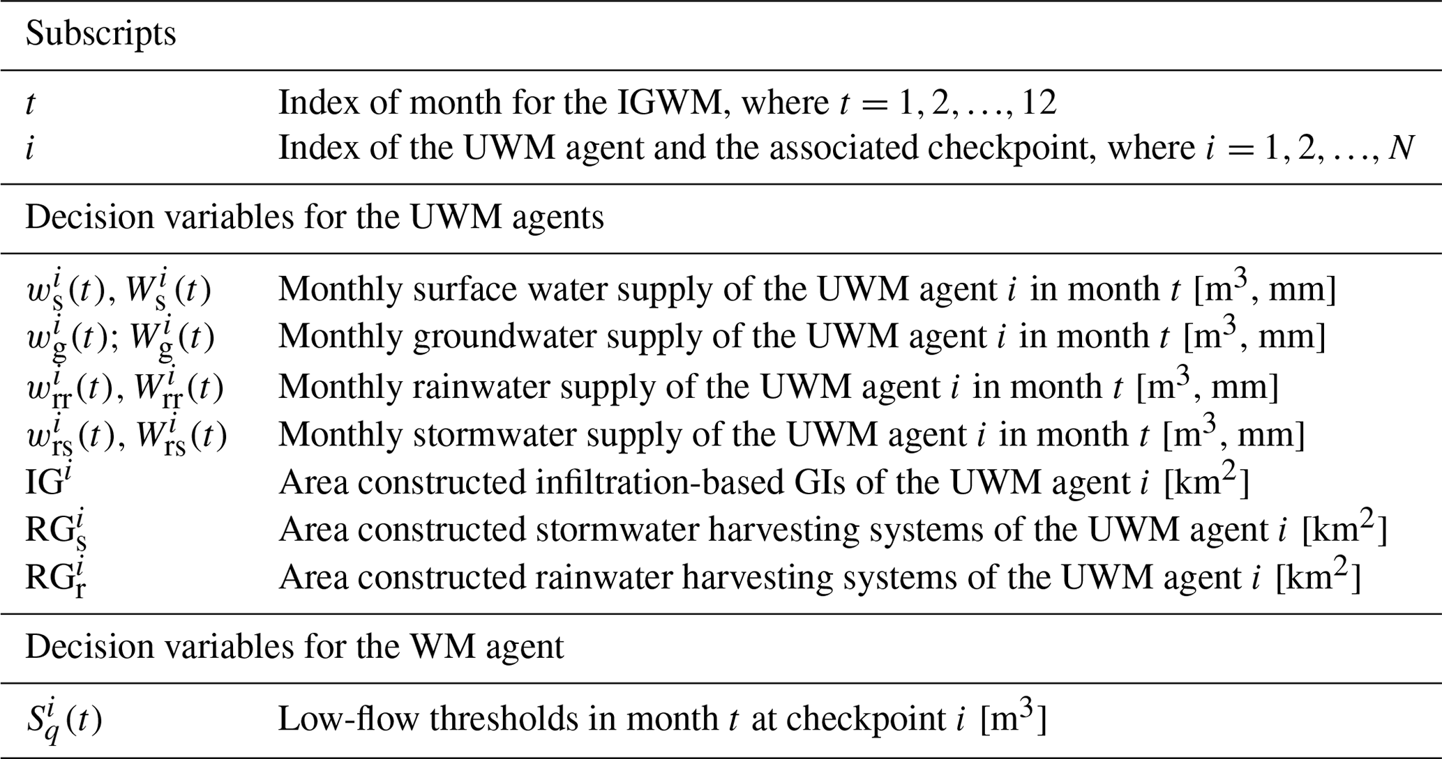
Table B2 Variables and parameters of the agent-based model for UWM.

Note that [–] represents dimensionless.

Table B3 Parameters of the agent-based model for WM.

B2 Agent-based model for UWM

Before model construction, the fundamental assumptions are given.

• Assumption 1. Three types of GIs can only be built in specific urban areas.

• Assumption 2. Four types of urban water demand need to be met via four types of water supply.

• Assumption 3. All water resources for supply can only be withdrawn or collected in urban areas.

• Assumption 4. The combined sewer system is considered in the urban system.

Some of these assumptions are imposed for the simplicity of the model. Assumption 1 describes urban land features and the space limitations for the development of three types of GIs, which is consistent with corresponding settings of the UWB-SM (see Fig. 3c). Assumption 2 is coherent with the associated hypothesis of the UWB-SM. Meanwhile, the irrigation demand of urban green space is also considered here. Assumption 3 indicates that inter-watershed water transfer schemes are not considered in the model for simplicity. Assumption 4 expresses that the model would take the sum of stormwater and wastewater into account in the calculation of urban wastewater drainage cost. The relevant decision variables and parameters of the agent-based model for UWM are listed in Tables B1 and B2, separately. Based on the above assumptions, using the UWM agent i as an example, the agent-based model for UWM model is formulated as a non-linear program as follows:

$$\begin{array}{}\text{(B1a)}& {\displaystyle }\underset{\mathrm{W},\mathrm{GI}}{min}{\mathrm{TC}}_i=C_{\mathrm{gi}}+C_{\mathrm{si}}+C_{\mathrm{wi}}\text{(B1b)}& {\displaystyle }\mathrm{s}.\mathrm{t}.\left\{\begin{array}{l}\begin{array}{lrr}{C}_{\mathrm{gi}}=c_{\mathrm{ig}}\cdot ({\mathrm{IG}}^i{)}^{e_{\mathrm{ig}}}+c_{\mathrm{rg}}\cdot ({\mathrm{RG}}_{\mathrm{r}}^i{)}^{e_{\mathrm{rg}}}+c_{\mathrm{sg}}\cdot ({\mathrm{RG}}_{\mathrm{s}}^i{)}^{e_{\mathrm{sg}}},& & \left(\mathrm{01}\right)\\ C_{\mathrm{si}}={\sum }_{t=\mathrm{1}}^{\mathrm{12}}[c_{\mathrm{ri}}\cdot w_{\mathrm{s}}^i(t{)}^{e_{\mathrm{ri}}}+c_{\mathrm{gi}}\cdot w_{\mathrm{g}}^i(t{)}^{e_{\mathrm{gi}}}+c_{\mathrm{rw}}\cdot w_{\mathrm{rr}}^i(t)+c_{\mathrm{sw}}\cdot w_{\mathrm{rs}}^i(t\left)\right],& & \left(\mathrm{02}\right)\\ C_{\mathrm{wi}}={\sum }_{t=\mathrm{1}}^{\mathrm{12}}{c}_{\mathrm{wd}}\cdot \left[q_{\mathrm{r}}\right(t)+q_{\mathrm{wd}}(t){]}^{e_{\mathrm{wd}}},& & \left(\mathrm{03}\right)\\ w_{\mathrm{s}}^i\left(t\right)=\mathrm{1000}\cdot A_{\mathrm{u}}^i\cdot W_{\mathrm{s}}^i\left(t\right),w_{\mathrm{g}}^i\left(t\right)=\mathrm{1000}\cdot A_{\mathrm{u}}^i\cdot W_{\mathrm{g}}^i\left(t\right),& \forall t& \left(\mathrm{04}\right)\\ w_{\mathrm{rr}}^i\left(t\right)=\mathrm{1000}\cdot A_{\mathrm{u}}^i\cdot W_{\mathrm{rr}}^i\left(t\right),w_{\mathrm{rs}}^i\left(t\right)=\mathrm{1000}\cdot A_{\mathrm{u}}^i\cdot W_{\mathrm{rs}}^i\left(t\right),& \forall t& \left(\mathrm{05}\right)\\ q_{\mathrm{r}}\left(t\right)=\mathrm{1000}\cdot A_{\mathrm{u}}^i\cdot \left[Q_{\mathrm{r}}\right(t){]}_{*},q_{\mathrm{wd}}(t)=\mathrm{1000}\cdot A_{\mathrm{u}}^i\cdot [Q_{\mathrm{wd}}\left(t\right){]}_{*},& \forall t& \left(\mathrm{06}\right)\\ \mathrm{0}\le {\mathrm{IG}}^i\le r_{\mathrm{imax}}\cdot A_{\mathrm{o}},\mathrm{0}\le {\mathrm{RG}}_{\mathrm{r}}^i\le r_{\mathrm{rmax}}\cdot A_{\mathrm{r}},\mathrm{0}\le {\mathrm{RG}}_{\mathrm{s}}^i\le r_{\mathrm{smax}}\cdot A_{\mathrm{u}},& & \left(\mathrm{07}\right)\\ \mathrm{0}\le W_{\mathrm{s}}^i\left(t\right)\le max[\mathrm{0},min(\left[S_{\mathrm{ri}}\right(t-\mathrm{1}){]}_{*}+Q_{\mathrm{ri}}(t)-S_{\mathrm{minr}},{\mathrm{WC}}_{\mathrm{ri}})],& \forall t& \left(\mathrm{08}\right)\\ \mathrm{0}\le W_{\mathrm{g}}^i\left(t\right)\le max[\mathrm{0},min(\left[S_{\mathrm{a}}\right(t-\mathrm{1}){]}_{*}-S_{\mathrm{mina}},{\mathrm{WC}}_{\mathrm{a}})],& \forall t& \left(\mathrm{09}\right)\\ \mathrm{0}\le W_{\mathrm{rr}}^i\left(t\right)\le \left[S_{\mathrm{gr}}\right(t-\mathrm{1}){]}_{*}+\frac{{\mathrm{RG}}_{\mathrm{r}}^i}{A_{\mathrm{u}}}\cdot P_{\mathrm{g}}(t),& \forall t& \left(\mathrm{10}\right)\\ \mathrm{0}\le W_{\mathrm{rs}}^i\left(t\right)\le \left[S_{\mathrm{gs}}\right(t-\mathrm{1}){]}_{*}+\frac{{\mathrm{RG}}_{\mathrm{s}}^i}{A_{\mathrm{u}}}\cdot [Q_{\mathrm{ru}}\left(t\right){]}_{*},& \forall t& \left(\mathrm{11}\right)\\ (\mathrm{1}-r_{\mathrm{dl}})\cdot \left[w_{\mathrm{s}}^i\right(t)+w_{\mathrm{g}}^i(t\left)\right]\ge D_{\mathrm{id}}\left(t\right),& \forall t& \left(\mathrm{12}\right)\\ (\mathrm{1}-r_{\mathrm{dl}})\cdot \left[w_{\mathrm{s}}^i\right(t)+w_{\mathrm{g}}^i(t\left)\right]+w_{\mathrm{rr}}^i\left(t\right)+w_{\mathrm{rr}}^i\left(t\right)\ge D_{\mathrm{id}}\left(t\right)+D_{\mathrm{in}}\left(t\right)+D_{\mathrm{o}}\left(t\right),& \forall t& \left(\mathrm{13}\right)\\ f_{\mathrm{sm}}\cdot (\mathrm{1}-[f_{\mathrm{sat}}\left(t\right){]}_{*})\cdot S_{\mathrm{smax}}\le [S_{\mathrm{s}}\left(t\right){]}_{*}& \forall t& \left(\mathrm{14}\right),\end{array}\end{array}\right.\end{array}$$

where $[-{]}_{*}$ represents the parameter being from simulation results of the UWB-SM. Equation (B1a) represents the objective function of the model, which aims to minimize the annual IGWM cost for the UWM agent. This cost is comprised of GI construction (C_gi), water supply (C_si), and wastewater drainage costs (C_wi). The calculation methods for these three costs are presented in the 1st to 3rd rows of Eq. (B1b). The 4th to 6th rows of Eq. (B1b) indicate the unit conversion process from millimeters [mm] to cubic meters [m³], which is essential for coupling the UWB-SM (using the unit mm) with the agent-based model for UWM (using the unit m³). The 7th row of Eq. (B1b) establishes the constraints for GI construction. Meanwhile, the 8th to 11th rows describe the water supply constraints for surface water, groundwater, rainwater, and stormwater withdrawals, respectively. Lastly, the 12th to 14th rows of the equation outline the water demand constraints concerning potable water demand, total water demand, and irrigation water demand. Notice that irrigation demand within urban areas only refers to the water needed for maintaining vegetation in both large-scale and small-scale infiltration-based GIs. Large-scale GIs include street trees, urban green spaces, parks, and gardens, while small-scale GIs encompass green roofs, rain gardens, and bioretention systems, etc. It can be estimated via using the minimum storage level of shallow soil layer for meeting basic water demands of plant.

B3 Agent-based model for WM

The agent-based model for WM is discussed in detail in the following. The relevant hypotheses for constructing the model are given.

• Assumption 1. The flow of each urban catchment at the outlet is checked.

• Assumption 2. Water withdrawal limit is not considered in the model.

Assumption 1 simplifies our models as WM set low-flow thresholds of each urban area at the outlet. For Assumption 2, computational complexity may be high in optimization of policy portfolio (setting water withdrawal limits and low-flow thresholds) for a WM agent model, especially when it is integrated into the multiagent system for UWMs. Also, a policy limiting the water withdrawal of urban areas, as a mandatory regulation, generally relies on other water users' activities within a watershed, such as agriculture sectors, which is beyond the scope of this study. Therefore, this paper considers water withdrawal limits (i.e., the minimum storage levels of aquifer and river) as UWM agent models' specific parameters (see the 8th and 9th rows of Eq. B1b).

As demonstrated in the above assumptions, a WM agent model is used to describe how a WM set a watershed management policy – a streamflow penalty strategy – to regulate all UWM agents' decision behavior of IGWM in a watershed. That is, a WM limits water abstraction decisions of each UWM agent in the period via prescribing a series of low streamflow thresholds in associated hydrological stations based on hydrologic states. If streamflow in the outlet for an urban area is below its threshold, a penalty fee will be imposed on the UWM agent. The strategy, in theory, can force UWM agents to recognize one or more of the externalities caused by IGWM, thereby adjusting their IGWM decisions because it can, to some extent, determine the cost of IGWM (Baumol and Oates, 1988). The WM can share fair water resources among urban areas in a watershed by setting a rational streamflow penalty strategy that affects all UWMs' decisions. Therefore, details of the objective and constraints of the agent-based model for WM are illustrated as follows.

Equity objective. The Gini coefficient is widely used to assess resource allocation inequality (Gini, 1921; Nishi et al., 2015). Therefore, the WM agent model uses a water allocation Gini coefficient index proposed by Hu et al. (2016) and Xu et al. (2019) – the equitable sharing of the used water quantity for each unit of cost – to measure equity of water sharing in watershed-scale IGWM. Based on the definition of the index, to minimize the Gini coefficient means maximal fairness of water resources distributions in a watershed; accordingly, the minimization of the equity objective for the WM can be expressed mathematically as follows:

$$\begin{array}{}\text{(B2)}& \begin{array}{rl}\underset{S_q^i}{min}\mathrm{Gini}& ={\displaystyle \frac{\mathrm{1}}{\mathrm{2}\cdot N\cdot \sum _{i=\mathrm{1}}^N\frac{\sum _{t=\mathrm{1}}^{\mathrm{12}}\left[w_{\mathrm{s}}^i\right(t)+w_{\mathrm{g}}^i(t)+w_{\mathrm{rr}}^i(t)+w_{\mathrm{rs}}^i(t\left)\right]}{{\mathrm{TC}}_i}}}\\ & \cdot \sum _{i=\mathrm{1}}^N\sum _{j=\mathrm{1}}^N|{\displaystyle \frac{\sum _{t=\mathrm{1}}^{\mathrm{12}}\left[w_{\mathrm{s}}^i\right(t)+w_{\mathrm{g}}^i(t)+w_{\mathrm{rr}}^i(t)+w_{\mathrm{rs}}^i(t\left)\right]}{{\mathrm{TC}}_i}}\\ & -{\displaystyle \frac{\sum _{t=\mathrm{1}}^{\mathrm{12}}\left[w_{\mathrm{s}}^j\right(t)+w_{\mathrm{g}}^j(t)+w_{\mathrm{rr}}^j(t)+w_{\mathrm{rs}}^j(t\left)\right]}{{\mathrm{TC}}_j}}|.\end{array}\end{array}$$

Streamflow constraints. The WM specifies the low streamflow thresholds at each checkpoint, which should adapt to actual hydrologic states. Therefore, the low streamflow thresholds at each checkpoint cannot exceed the associated maximal historical streamflow and cannot be below the minimal one in each month:

$$\begin{array}{}\text{(B3)}& {\mathrm{SQ}}_{\min }^i\left(t\right)\le S_q^i\le {\mathrm{SQ}}_{\max }^i\left(t\right),\forall t,i.\end{array}$$

In short, the WM agent model is represented as follows:

$$\begin{array}{}\text{(B4a)}& {\displaystyle }\begin{array}{rl}\underset{S_q^i}{min}\mathrm{Gini}& ={\displaystyle \frac{\mathrm{1}}{\mathrm{2}\cdot N\cdot \sum _{i=\mathrm{1}}^N\frac{\sum _{t=\mathrm{1}}^{\mathrm{12}}\left[w_{\mathrm{s}}^i\right(t)+w_{\mathrm{g}}^i(t)+w_{\mathrm{rr}}^i(t)+w_{\mathrm{rs}}^i(t\left)\right]}{T{C}_i}}}\\ & \cdot \sum _{i=\mathrm{1}}^N\sum _{j=\mathrm{1}}^N|{\displaystyle \frac{\sum _{t=\mathrm{1}}^{\mathrm{12}}\left[w_{\mathrm{s}}^i\right(t)+w_{\mathrm{g}}^i(t)+w_{\mathrm{rr}}^i(t)+w_{\mathrm{rs}}^i(t\left)\right]}{{\mathrm{TC}}_i}}\\ & -{\displaystyle \frac{\sum _{t=\mathrm{1}}^{\mathrm{12}}\left[w_{\mathrm{s}}^j\right(t)+w_{\mathrm{g}}^j(t)+w_{\mathrm{rr}}^j(t)+w_{\mathrm{rs}}^j(t\left)\right]}{{\mathrm{TC}}_j}}|\end{array}\text{(B4b)}& {\displaystyle }\mathrm{s}.\mathrm{t}.\left\{\begin{array}{l}{\mathrm{SQ}}_{\min }^i\left(t\right)\le S_q^i\left(t\right)\le {\mathrm{SQ}}_{\max }^i\left(t\right),\forall t,i.\end{array}\right.\end{array}$$

Appendix C: Details of two hydrologic models

This appendix comprehensively elucidates the details of two hydrologic models – UWB-SM and Muskingum–Cunge routing model. It is described from various aspects including the notation, the UWB-SM, and the Muskingum–Cunge routing model.

C1 Notation

To facilitate the model presentation, some of the important notation used hereafter is summarized in Tables C1–C6.

Table C1 Urban water demand and the hydroclimatic input parameters of the UWB-SM.

Table C2 Measured parameters of the UWB-SM.

Table C3 Calibration parameters of the UWB-SM.

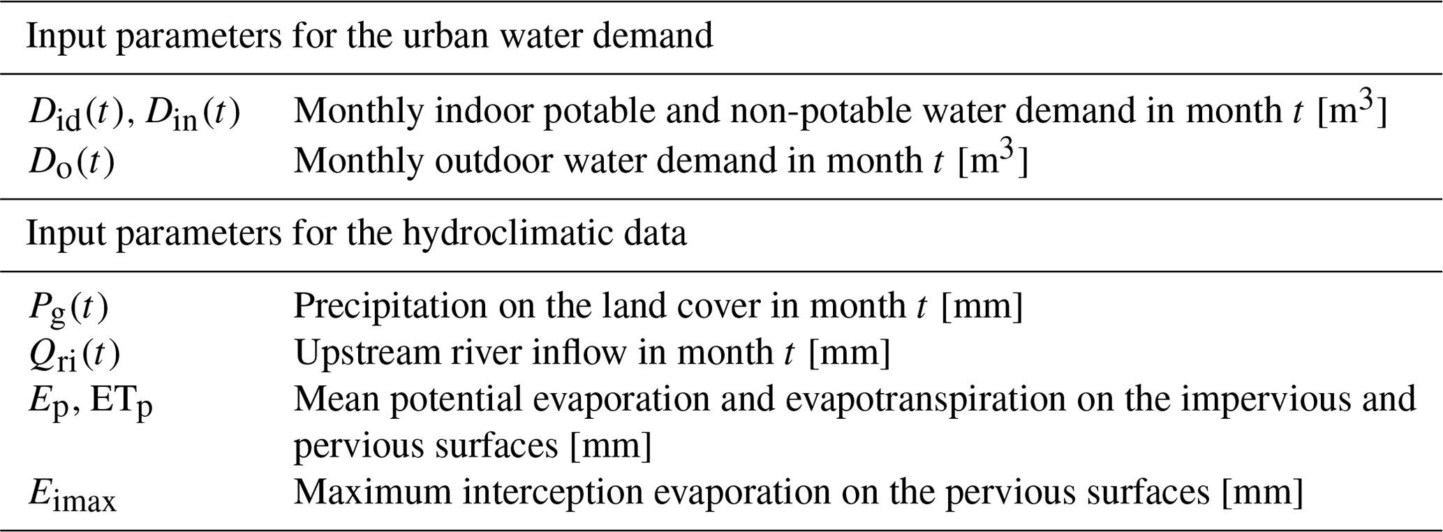
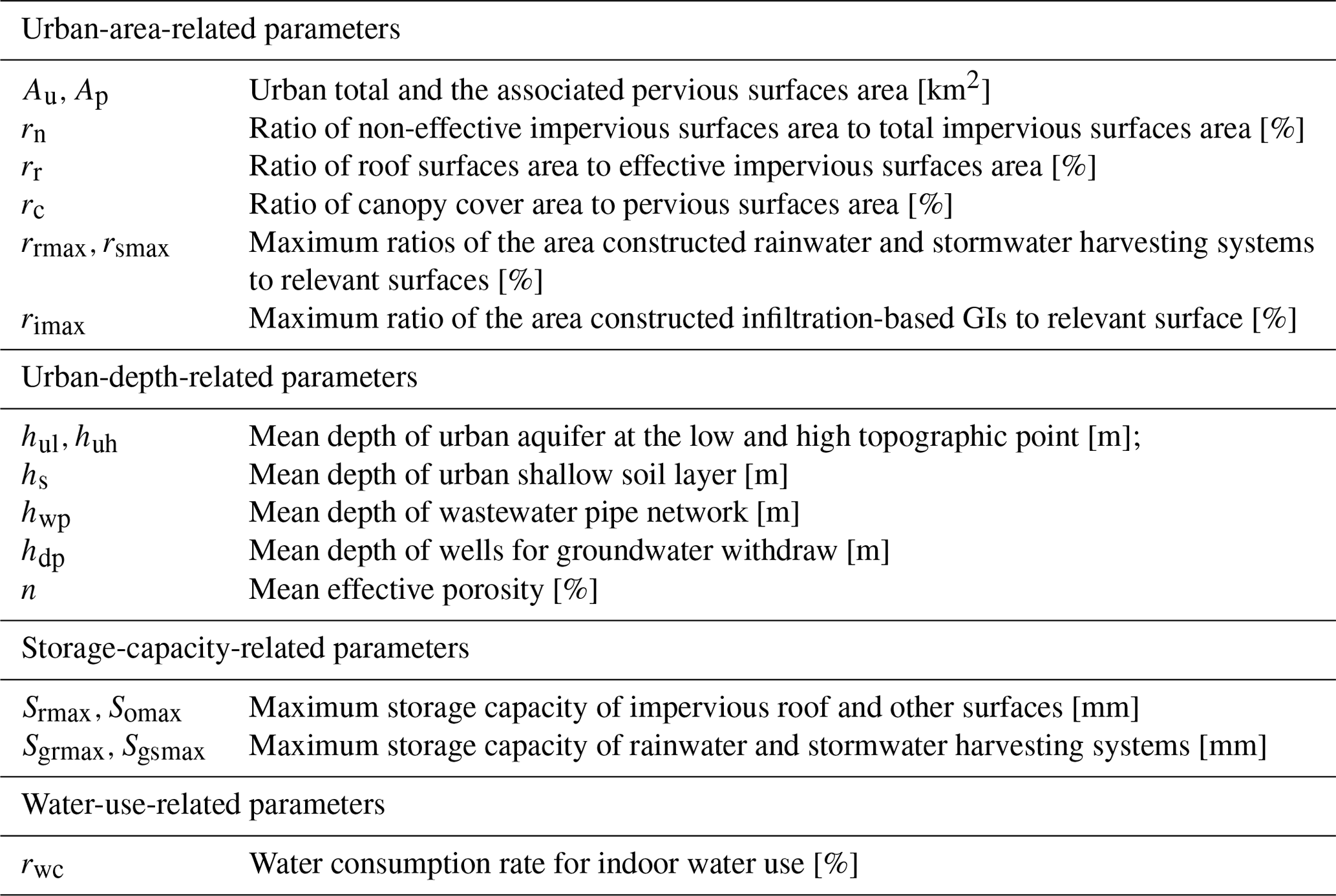
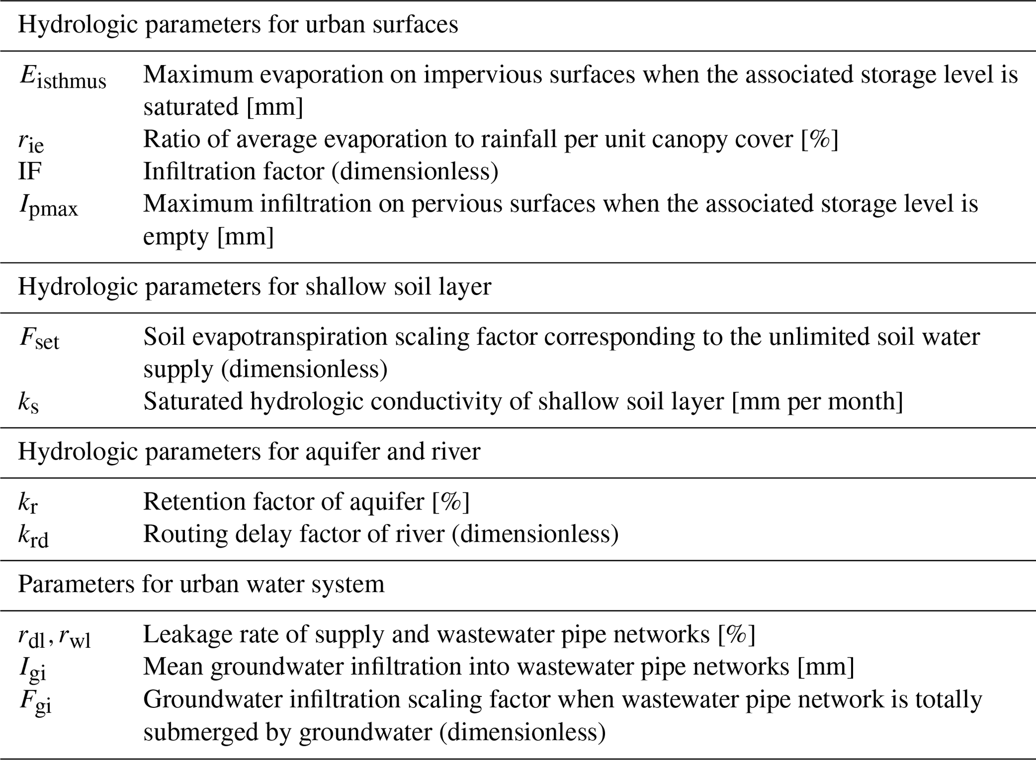
Table C4 Urban-surface-related variables and parameters of the UWB-SM.

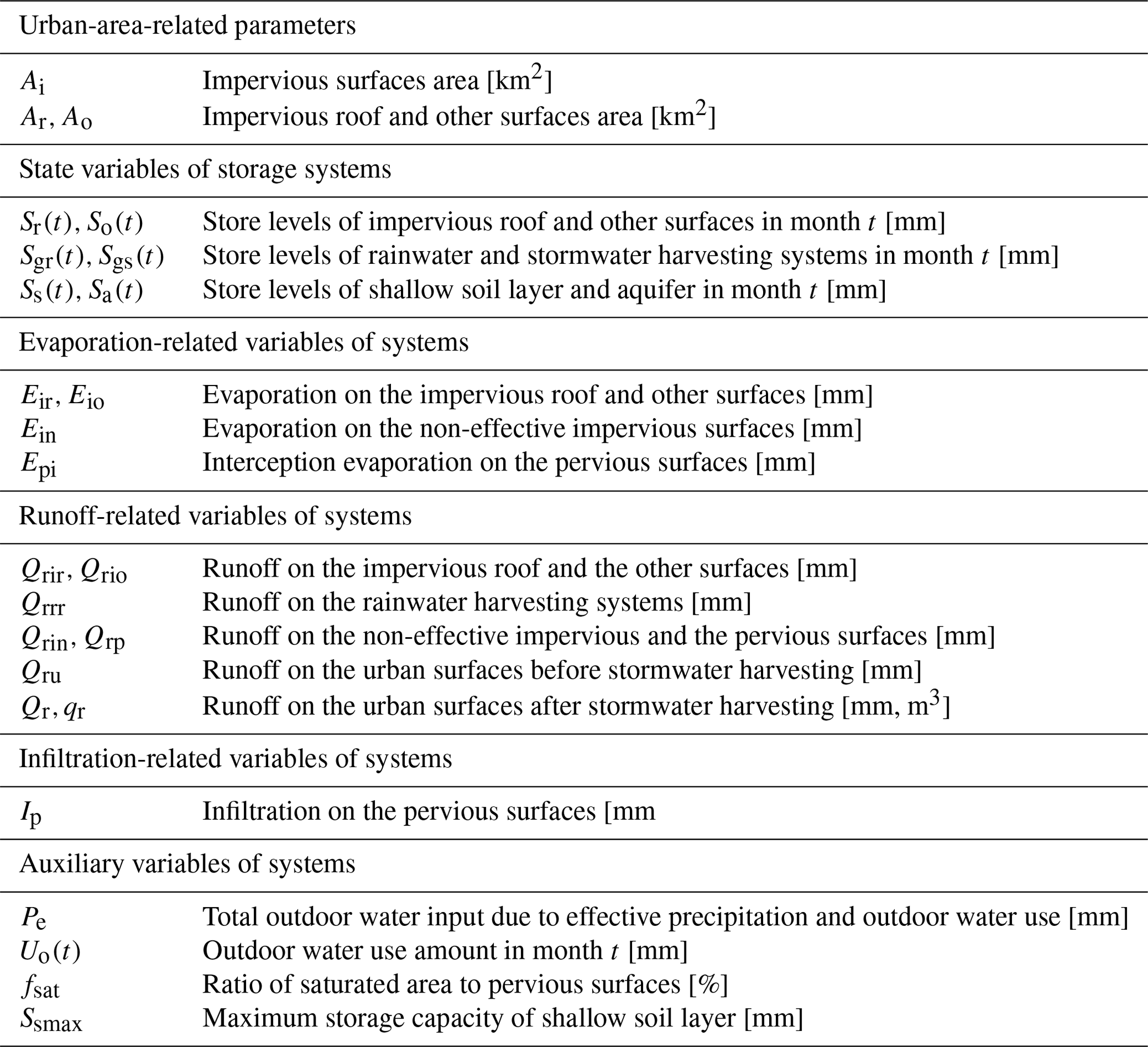
Table C5 Underground and river-related variables and parameters of the UWB-SM.

Table C6 Parameters of the Muskingum–Cunge routing model.

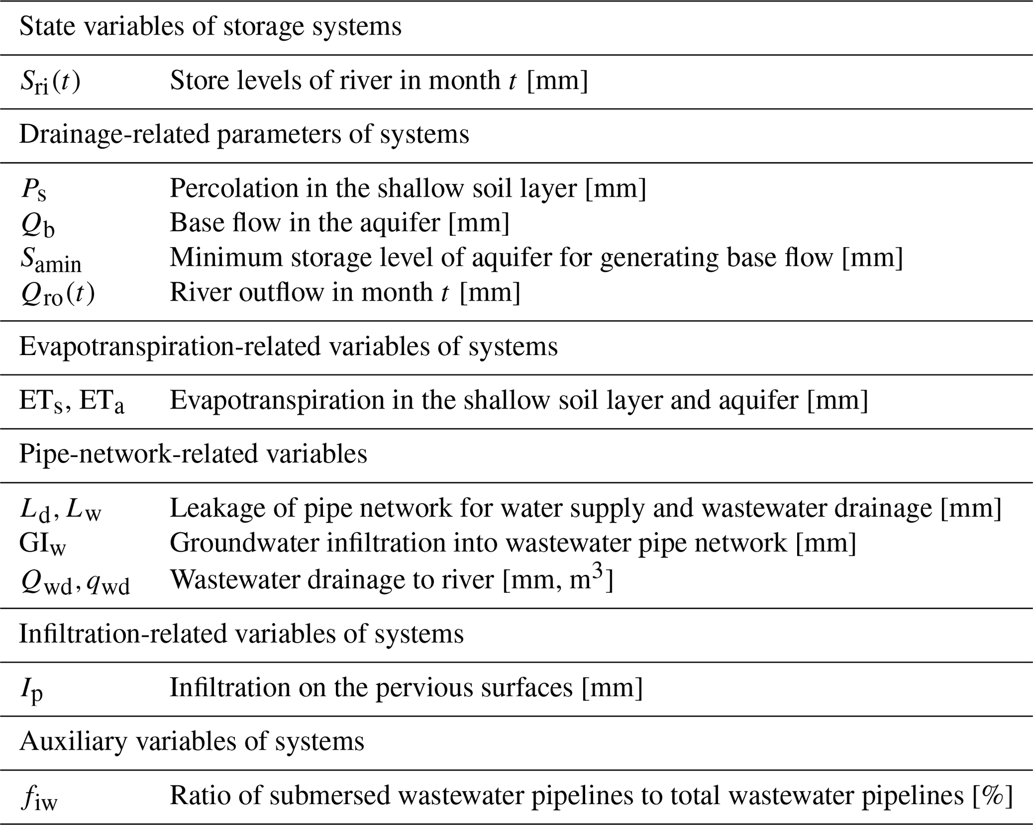
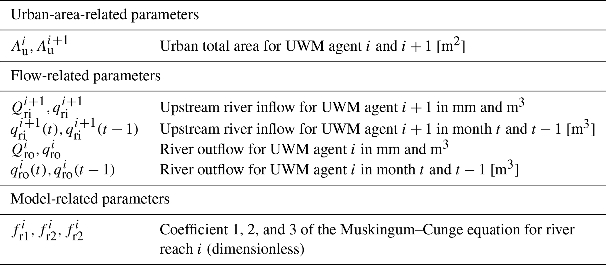
C2 Urban water balance simulation model

Details of the governing equations for the UWB-SM are shown in the following.

Urban surfaces. In the UWB-SM, we assume that precipitation is distributed evenly over the entire area and does not take urban spatial features into account due to the limited monthly impact on urban water management decisions. By the assumption, the amounts of rainfall on different urban surfaces can be calculated by ratios of relevant surface areas to the urban area's multiple gross precipitations. Notice that the pervious surface receives input from effective precipitation, outdoor water use, and surface runoff from adjacent impervious areas. The effective precipitation is defined by the relevant gross precipitation minus the interception and evaporation on the plant cover area within the region. For the infiltration process, the infiltration and saturation excess are modeled to calculate the runoff and the infiltration according to the soil moisture conditions. The impervious and pervious surface runoff flows into the drains, collected by stormwater harvesting systems. The rest discharges into the river. The relevant terms and units are defined in Table C4. Taking the IGWM decisions of UWM agent i in month t as an example, the detail of the hydrologic process on the urban surface is formulated in the following.

Hydrologic process on the impervious roof surfaces. The water mass balance equation for the impervious roof surfaces can be expressed as

$$\begin{array}{}\text{(C1)}& S_{\mathrm{r}}\left(t\right)-S_{\mathrm{r}}(t-\mathrm{1})=P_{\mathrm{g}}\left(t\right)-E_{\mathrm{ir}}\left(t\right)-Q_{\mathrm{rir}}\left(t\right),\end{array}$$

where the roof area $A_{\mathrm{r}}=r_{\mathrm{r}}\cdot (A_{\mathrm{u}}-A_{\mathrm{p}})$, P_g(t) represents precipitation on the impervious roof surfaces, and evaporation can be calculated by $E_{\mathrm{ir}}\left(t\right)=max[E_{\mathrm{ismax}}\cdot \frac{S_{\mathrm{r}}(t-\mathrm{1})}{S_{\mathrm{rmax}}},E_{\mathrm{p}}(t\left)\right]$ based on the equation by Mitchell et al. (2001). And the storage levels is updated by a reservoir model; $S_{\mathrm{r}}\left(t\right)=min\left[S_{\mathrm{r}}\right(t-\mathrm{1})+P_{\mathrm{g}}(t)-E_{\mathrm{ir}}(t),S_{\mathrm{rmax}}]$.

Hydrologic process on the other impervious surfaces. Similar to the impervious roof surfaces, the water mass balance formulation for the other impervious surfaces is shown as

$$\begin{array}{}\text{(C2)}& S_{\mathrm{o}}\left(t\right)-S_{\mathrm{o}}(t-\mathrm{1})=P_{\mathrm{g}}\left(t\right)-E_{\mathrm{io}}\left(t\right)-Q_{\mathrm{rio}}\left(t\right),\end{array}$$

where the other impervious surfaces area A_o is equal to $(\mathrm{1}-r_{\mathrm{r}})\cdot (A_{\mathrm{u}}-A_{\mathrm{p}})$, and the calculation of the evaporation is also dependent on the Mitchell et al. (2001) method; $E_{\mathrm{io}}\left(t\right)=max[E_{\mathrm{ismax}}\cdot \frac{S_{\mathrm{o}}(t-\mathrm{1})}{S_{\mathrm{omax}}},E_{\mathrm{p}}(t\left)\right]$. The update of relevant storage levels, S_o(t), is equal to $min\left[S_{\mathrm{o}}\right(t-\mathrm{1})+P_{\mathrm{g}}(t)-E_{\mathrm{io}}(t),S_{\mathrm{omax}}]$.

Hydrologic process for the rainwater harvesting systems. In the rainwater harvesting systems, evaporation is ignored because of the assumption that rainwater is collected rapidly and storage is sealed. We can draw its mass balance relationship as follows:

$$\begin{array}{}\text{(C3)}& S_{\mathrm{gr}}\left(t\right)-S_{\mathrm{gr}}(t-\mathrm{1})=P_{\mathrm{g}}\left(t\right)-W_{\mathrm{rr}}^i\left(t\right)-Q_{\mathrm{rrr}}\left(t\right),\end{array}$$

where $W_{\mathrm{rr}}^i\left(t\right)$ is obtained from the unit conversion from cubic meters to millimeters, which is equal to $\frac{w_{\mathrm{rr}}^i\left(t\right)}{\mathrm{1000}\cdot R{G}_{\mathrm{r}}^i}$, and the updated storage levels of the system S_gr(t) are equivalent to $min\left[S_{\mathrm{gr}}\right(t-\mathrm{1})+P_{\mathrm{g}}(t)-W_{\mathrm{rr}}^i(t),S_{\mathrm{grmax}}]$.

Hydrologic process on the non-effective area. Hydrologic process on the non-effective area: for the simplicity of the model, it assumed that rainfall only generates runoff and evaporation on the non-effective area. This study calculates the corresponding runoff based on the following equation – $Q_{\mathrm{rin}}\left(t\right)=r_{\mathrm{n}}\cdot [\frac{A_{\mathrm{r}}}{A_{\mathrm{i}}}\cdot Q_{\mathrm{rir}}(t)+\frac{A_{\mathrm{r}}-{\mathrm{RG}}_{\mathrm{r}}}{A_{\mathrm{i}}}\cdot Q_{\mathrm{rio}}(t)+\frac{A_{\mathrm{o}}-\mathrm{IG}}{A_{\mathrm{i}}}\cdot Q_{\mathrm{rrr}}(t\left)\right]$, where the impervious area $A_{\mathrm{i}}=A_{\mathrm{u}}-A_{\mathrm{p}}-\mathrm{IG}$.

$$\begin{array}{}\text{(C4)}& P_{\mathrm{g}}\left(t\right)=Q_{\mathrm{rin}}\left(t\right)+E_{\mathrm{in}}\left(t\right).\end{array}$$

Hydrologic process on the pervious surfaces. The water mass conservation equation for the pervious surfaces is represented as follows:

$$\begin{array}{}\text{(C5)}& Q_{\mathrm{rin}}\left(t\right)+P_{\mathrm{g}}\left(t\right)+U_{\mathrm{o}}\left(t\right)=Q_{\mathrm{rp}}\left(t\right)+E_{\mathrm{pi}}\left(t\right)+I_{\mathrm{p}}\left(t\right).\end{array}$$

The right side of Eq. (C5) donates the inflow on the pervious surface, including runoff from the non-effective area, precipitation, and outdoor water use. The outdoor water use is the total amount of water supply minus indoor water demand: $U_{\mathrm{o}}\left(t\right)=(\mathrm{1}-r_{\mathrm{dl}})\cdot \left[W_{\mathrm{s}}^i\right(t)+W_{\mathrm{g}}^i(t\left)\right]+W_{\mathrm{rr}}^i\left(t\right)+W_{\mathrm{rs}}^i\left(t\right)-\frac{d_{\mathrm{ip}}\left(t\right)+d_{\mathrm{in}}\left(t\right)}{\mathrm{1000}\cdot A_{\mathrm{u}}^i}$, where $W_{\mathrm{s}}^i\left(t\right)$, $W_{\mathrm{g}}^i\left(t\right)$, and $W_{\mathrm{rs}}^i\left(t\right)$ are obtained from the unit conversion from m³ to mm and are equal to $\frac{w_{\mathrm{s}}^i\left(t\right)}{\mathrm{1000}\cdot A_{\mathrm{u}}^i}$, $\frac{w_{\mathrm{g}}^i\left(t\right)}{\mathrm{1000}\cdot A_{\mathrm{u}}^i}$, and $\frac{w_{\mathrm{rs}}^i\left(t\right)}{\mathrm{1000}\cdot {\mathrm{RG}}_{\mathrm{s}}^i}$.

The left-hand side of Eq. (C5) represents outflow on the pervious surfaces, consisting of runoff, interception evaporation, and infiltration, separately. Interception evaporation is calculated based on urban vegetation canopy area and associated features, following Van Dijk and Bruijnzeel (2001) approach – $E_{\mathrm{pi}}\left(t\right)=min[r_{\mathrm{c}}\cdot r_{\mathrm{ie}}\cdot \cdot P_{\mathrm{g}}(t),E_{\mathrm{imax}}]$. The calculation of infiltration is based on two hydrologic processes: saturated and infiltration excess (Viney et al., 2015). We assume that there would be no infiltration on the saturated area within the pervious surface, and its ratio $f_{\mathrm{sat}}\left(t\right)=max\left[\frac{\frac{S_{\mathrm{a}}(t-\mathrm{1})}{\mathrm{1000}\cdot n}-h_{\mathrm{ul}}}{h_{\mathrm{uh}}-h_{\mathrm{ul}}},\mathrm{0}\right]$ (see Fig. 3b). For the other part – an unsaturated area – an infiltration rate is estimated using an exponential function of storage levels of the shallow soil layer (Chiew and McMahon, 1999); the infiltration is minimum when the storage level is saturated and continuously increases to a maximum when the storage level is empty. Therefore, the formulation of infiltration is $I_{\mathrm{p}}\left(t\right)=[\mathrm{1}-f_{\mathrm{sat}}(t\left)\right]\cdot max[I_{\mathrm{pmax}}\cdot e^{-\mathrm{IF}\cdot \frac{S_{\mathrm{s}}(t-\mathrm{1})}{S_{\mathrm{smax}}}},P_{\mathrm{e}}(t)+Q_{\mathrm{rin}}(t\left)\right]$, where maximum storage capacity of shallow soil layer $S_{\mathrm{smax}}=\mathrm{1000}\cdot n\cdot h_{\mathrm{s}}$ and total outdoor water input $P_{\mathrm{e}}\left(t\right)=P_{\mathrm{g}}\left(t\right)+U_{\mathrm{o}}\left(t\right)-E_{\mathrm{pi}}\left(t\right)$.

Hydrologic process for the stormwater harvesting systems. Similar to rainwater harvesting systems, stormwater harvesting systems are also hypothesized to have no evaporation. Its mass balance equation can be represented by

$$\begin{array}{}\text{(C6)}& S_{\mathrm{gs}}\left(t\right)-S_{\mathrm{gs}}(t-\mathrm{1})=Q_{\mathrm{ru}}\left(t\right)-W_{\mathrm{rs}}^i\left(t\right)-Q_{\mathrm{r}}\left(t\right),\end{array}$$

where runoff that is available for collection is the sum of runoff from the effective impervious and the pervious surfaces – $Q_{\mathrm{ru}}=Q_{\mathrm{rp}}\left(t\right)+(\mathrm{1}-r_{\mathrm{n}})\cdot [\frac{A_{\mathrm{r}}}{A_{\mathrm{i}}}\cdot Q_{\mathrm{rir}}(t)+\frac{A_{\mathrm{r}}-{\mathrm{RG}}_{\mathrm{r}}}{A_{\mathrm{i}}}\cdot Q_{\mathrm{rio}}(t)+\frac{A_{\mathrm{o}}-\mathrm{IG}}{A_{\mathrm{i}}}\cdot Q_{\mathrm{rrr}}(t)$]. The relevant storage levels can be updated by $S_{\mathrm{gs}}\left(t\right)=min\left[S_{\mathrm{gs}}\right(t-\mathrm{1})+Q_{\mathrm{ru}}-W_{\mathrm{rs}}^i(t),S_{\mathrm{gsmax}}]$.

Shallow soil layer. As shown in Fig. 3b, a non-linear reservoir model with the depth h_s is given to describe relevant hydrologic processes in the shallow soil layer. The shallow soil layer receives water from the urban surfaces by infiltration and drains water by percolation into the aquifer and evapotranspiration to the atmosphere. Therefore, the water mass balance equation for the shallow soil layer can be written as

$$\begin{array}{}\text{(C7)}& S_{\mathrm{s}}\left(t\right)-S_{\mathrm{s}}(t-\mathrm{1})=I_{\mathrm{p}}\left(t\right)-P_{\mathrm{s}}\left(t\right)-{\mathrm{ET}}_{\mathrm{s}}\left(t\right),\end{array}$$

where percolation is assumed to occur according to the following equation by Frost et al. (2016) for the shallow soil layer: $P_{\mathrm{s}}\left(t\right)=k_{\mathrm{s}}\cdot [\frac{S_{\mathrm{s}}(t-\mathrm{1})}{S_{\mathrm{smax}}}{]}^{\mathrm{2}}$. The evapotranspiration process occurs in the unsaturated portion of the shallow soil layer, and it can be given by using the Frost et al. (2016) method: ET${}_{\mathrm{s}}\left(t\right)=[\mathrm{1}-f_{\mathrm{sat}}(t\left)\right]\cdot F_{set}\cdot {\mathrm{ET}}_{\mathrm{p}}\left(t\right)\cdot min[\frac{S_{\mathrm{s}}(t-\mathrm{1})+I_{\mathrm{p}}\left(t\right)}{S_{\mathrm{smax}}},\mathrm{1}]$.

Aquifer. In the UWB-SM, the only unconfined aquifer is considered a linear reservoir model to simulate groundwater-related hydrologic dynamics (Mitchell et al., 2001), indicating that there is no deep seepage from the aquifer. The aquifer receives water from percolation and leakage of water supply and wastewater pipelines and discharges water in the manners of base flow, evapotranspiration, groundwater extraction for use, and infiltration into wastewater pipelines (Ellis, 2001). Hence, the mass balance formulation of aquifer can be expressed as

$$\begin{array}{}\text{(C8)}& \begin{array}{rl}{S}_{\mathrm{a}}\left(t\right)& -S_{\mathrm{a}}(t-\mathrm{1})=P_{\mathrm{s}}\left(t\right)+L_{\mathrm{d}}\left(t\right)+L_{\mathrm{w}}\left(t\right)-{\mathrm{GI}}_{\mathrm{w}}\left(t\right)\\ & -W_{\mathrm{g}}^i\left(t\right)-{\mathrm{ET}}_{\mathrm{a}}\left(t\right)-Q_{\mathrm{b}}\left(t\right),\end{array}\end{array}$$

where the leakage of water supply pipe networks is $L_{\mathrm{d}}\left(t\right)=r_{\mathrm{dl}}\cdot \left[W_{\mathrm{rr}}^i\right(t)+W_{\mathrm{rs}}^i(t\left)\right]$, and the calculation of the sewer pipelines infiltration and exfiltration (leakage) is by comparing the depth of wastewater pipelines with groundwater table (Wolf, 2006) – groundwater would infiltrate into wastewater pipelines when the pipe is below the groundwater table, whereas wastewater would leak into the aquifer from pipelines when the pipe is above the level of the groundwater table. Figure 3c illustrates that the fraction of the sewer pipelines that is below the groundwater table is defined as $f_{\mathrm{iw}}\left(t\right)=max[\frac{\frac{S_{\mathrm{a}}(t-\mathrm{1})}{\mathrm{1000}\cdot n}+h_{\mathrm{wp}}-h_{\mathrm{ul}}}{h_{\mathrm{uh}}-h_{\mathrm{ul}}},\mathrm{0}]$, which is used to calculate the sewer pipelines infiltration GI${}_{\mathrm{w}}\left(t\right)=f_{\mathrm{iw}}\left(t\right)\cdot I_{\mathrm{gi}}\cdot F_{\mathrm{gi}}$ via using Wolf (2006) method, and the associated exfiltration part of pipe networks $L_{\mathrm{w}}\left(t\right)=r_{\mathrm{wl}}\cdot (\mathrm{1}-r_{\mathrm{wc}})\cdot (\mathrm{1}-f_{\mathrm{iw}}(t\left)\right)\cdot \left[\frac{d_{\mathrm{ip}}\left(t\right)+d_{\mathrm{in}}\left(t\right)}{\mathrm{1000}\cdot A_{\mathrm{u}}^i}\right]$ though applying the Mitchell et al. (2001) equation. The evapotranspiration in the aquifer occurs in the saturated portion of the shallow soil layer (Fig. 3c), which can also be computed according to the Frost et al. (2016) method: ET${}_{\mathrm{a}}\left(t\right)=f_{\mathrm{sat}}\left(t\right)\cdot F_{\mathrm{set}}\cdot {\mathrm{ET}}_p\left(t\right)$. The amount of base flow is assumed to be linearly proportional to the storage level of the aquifer (Fenicia et al., 2006) - $Q_{\mathrm{b}}\left(t\right)=max[k_{\mathrm{r}}\cdot (S_{\mathrm{a}}(t-\mathrm{1})-S_{\mathrm{amin}}),\mathrm{0}]$, where $S_{\mathrm{amin}}=\mathrm{1000}\cdot n\cdot h_{\mathrm{ul}}$.

River. We assume that the “River” component of the UWBv-SM includes all surface water bodies within an urban area. It accepts water from upstream inflow, runoff within the urban surfaces, and base flow from the aquifer and drains water to the adjacent downstream region. In addition, an urban area can withdraw water from the river and discharge wastewater into it. So, the water mass conservation equation for a river can written as

$$\begin{array}{}\text{(C9)}& \begin{array}{rl}{S}_{\mathrm{ri}}\left(t\right)& -S_{\mathrm{ri}}(t-\mathrm{1})=Q_{\mathrm{ri}}\left(t\right)+Q_{\mathrm{r}}\left(t\right)+Q_{\mathrm{b}}\left(t\right)+Q_{\mathrm{wd}}\left(t\right)\\ & -W_{\mathrm{s}}^i\left(t\right)-Q_{\mathrm{ro}}\left(t\right),\end{array}\end{array}$$

where total wastewater drainage is calculated as the sum of indoor water drainage and sewer infiltration and sewer leakage have been subtracted: $Q_{\mathrm{wd}}=(\mathrm{1}-r_{\mathrm{wc}})\cdot \left[\frac{d_{\mathrm{ip}}\left(t\right)+d_{\mathrm{in}}\left(t\right)}{\mathrm{1000}\cdot A_{\mathrm{u}}^i}\right]+{\mathrm{GI}}_{\mathrm{w}}\left(t\right)-L_{\mathrm{w}}\left(t\right)$. The outflow of the river is routed via a notional river store level, which can be controlled by a routing delay factor (k_rd ) according to the Frost et al. (2016) equation: $Q_{\mathrm{ro}}\left(t\right)=(\mathrm{1}-e^{-k_{\mathrm{rd}}})\cdot \left[S_{\mathrm{s}}\right(t-\mathrm{1})+Q_{\mathrm{ri}}(t)+Q_{\mathrm{r}}(t)+Q_{\mathrm{b}}(t)+Q_{\mathrm{wd}}(t)-W_{\mathrm{s}}^i(t\left)\right]$.

C3 Muskingum–Cunge routing model

Figure 1b illustrates the upstream–downstream hydrologic interaction between UWM agent i and i+1 in the associated river reach. A Muskingum–Cunge routing model is used to simulate changes in streamflow in the river reach connected with two adjacent urban areas (Garbrecht and Brunner, 1991; Weinmann and Laurenson, 1979). Figure. 1b illustrates the upstream–downstream hydrologic interaction between UWM agent i and i+1 in the associated river reach. A Muskingum–Cunge routing equation is used to simulate changes in streamflow in the river reach connected with two adjacent urban areas (Garbrecht and Brunner, 1991; Weinmann and Laurenson, 1979). That is, taking the UWM agent i+1 in month t as an example (see Fig. 1b), its upstream inflow in month t can be expressed mathematical by outflow of the UWM agent i in month t and t+1, as follows:

$$\begin{array}{}\text{(C10)}& \left\{\begin{array}{lr}{q}_{\mathrm{ri}}^{i+\mathrm{1}}\left(t\right)=f_{\mathrm{r}\mathrm{1}}^i\cdot q_{\mathrm{ro}}^i\left(t\right)+f_{\mathrm{r}\mathrm{2}}^i\cdot q_{\mathrm{ro}}^i(t-\mathrm{1})+f_{\mathrm{r}\mathrm{3}}^i\cdot q_{\mathrm{ri}}^{i+\mathrm{1}}(t-\mathrm{1}),& \left(\mathrm{01}\right)\\ q_{\mathrm{ro}}^i\left(t\right)=\mathrm{1000}\cdot A_{\mathrm{u}}^i\cdot \left[Q_{\mathrm{ro}}^i\right(t){]}_{*},& \left(\mathrm{02}\right)\\ q_{\mathrm{ri}}^{i+\mathrm{1}}\left(t\right)=\mathrm{1000}\cdot A_{\mathrm{u}}^{i+\mathrm{1}}\cdot Q_{\mathrm{ri}}^{i+\mathrm{1}}\left(t\right),& \left(\mathrm{03}\right)\end{array}\right.\end{array}$$

where all parameters of the above notation are listed in Table C6. The first row of Eq. (C10) is the Muskingum–Cunge model for calculating the relevant river reach inflow of downstream agents. The second and third rows of Eq. (C10) represent the units for hydrological parameters being converted from millimeters to cubic meters based on the associated urban total areas. In addition, it should be noted that the Muskingum–Cunge approach is also applicable in the case that there are branches in the main river reach (see UWM agents 1, 2 and 3 in Fig. 1a), which can be solved by dividing the river reach into several sub-reaches based on intersections of the main river and associated branches and then calculating them in sequence.

Appendix D: Details of the agent-based model for city-scale IGWM

This appendix comprehensively elucidates the details of the relevant solution approach pertaining to the agent-based model for city-scale IGWM – simulation-based adaptive particle swarm optimization (S-APSO). It is meticulously described from various aspects including the notation and the solution approaches pertaining to this model.

D1 Notation

To facilitate the model presentation, some of the important notation used hereafter is summarized in Table D1.

Table D1 Parameters of the S-APSO.

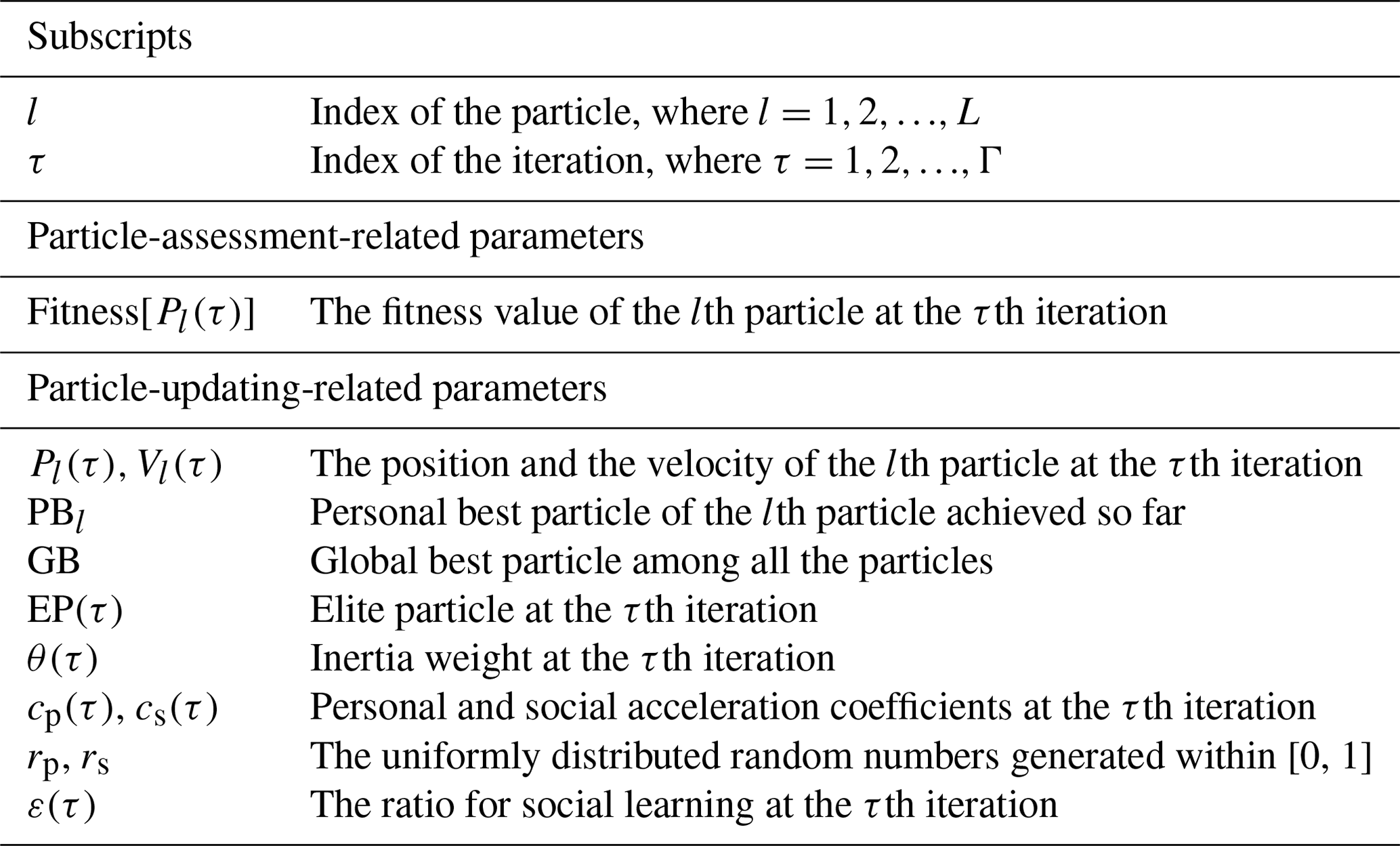
D2 Solution approach

Unlike traditional water management models (Loucks and Van Beek, 2017), it might be hard to solve the agent-based model, which consists of the agent-based model for UWM (Eq. B1) and UWB-SM, via using general methods, because of the non-linearity of its objective function and complexity of its solution space induced by coupling with the UWB-SM. To solve complex water resources management problems, heuristic search-based techniques, such as particle swarm optimization (PSO) that is a swarm-based intelligence method to search for globally optimal solutions via imitating swarm behavior in birds flocking (Kennedy and Eberhart, 1995), are widely applied and developed (Nicklow et al., 2010; Chang et al., 2013). Therefore, in this study, according to features of the UWM agent model, a simulation-based adaptive particle swarm optimization (S-APSO) is designed, and its flowchart diagram is illustrated in Fig. D1a. As shown in Fig. D1a, compared with particle initialization and evaluation for standard PSO, a coupling procedure proposed above for data exchange between an agent-based model for UWM and UWB-SM is nested to make sure all particles feasible and measurable. Compared with the standard PSO updating mechanism, a Boltzmann selection operator and an evolutionary state-based parameter adaptation scheme are added to avoid premature convergence to improve algorithm performance; a simulation-based check and repair mechanism is introduced to guarantee that all particles are feasible during the particle updating process. These key features of the proposed S-APSO are explained in the following.

Figure D1 Flowchart diagram of the S-APSO for agent-based model for city-scale IGWM.

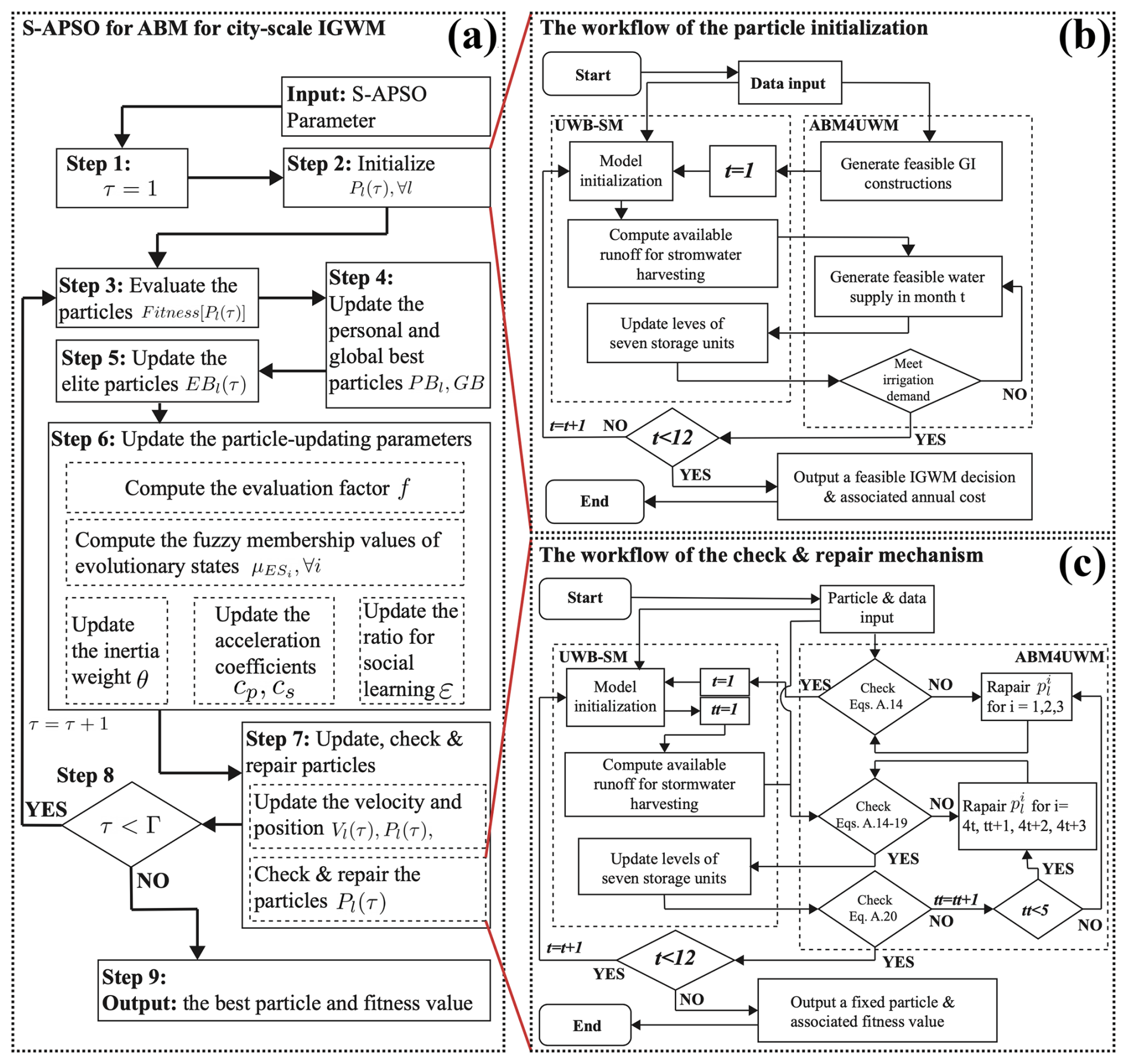
Solution representation and particle performance calculation. In the S-APSO, a particle representing a feasible solution of the Eq. (B1) can be encoded as an array with 51 dimensions, which indicates 3 GI construction variables and 4 × 12 monthly water supply variables, respectively. It can be written as follows:

$$\begin{array}{}\text{(D1)}& \begin{array}{rl}{P}_l\left(\mathit{\tau }\right)& =\left[p_l^{\mathrm{1}}\right(\mathit{\tau }),p_l^{\mathrm{2}}(\mathit{\tau }),p_l^{\mathrm{3}}(\mathit{\tau }),p_l^{\mathrm{4}}(\mathit{\tau }),p_l^{\mathrm{5}}(\mathit{\tau }),p_l^{\mathrm{6}}(\mathit{\tau }),p_l^{\mathrm{7}}(\mathit{\tau }),\\ & \mathrm{\dots },p_l^{\mathrm{51}}\left(\mathit{\tau }\right)]\\ & \leftrightarrow [{\mathrm{IG}}^i,{\mathrm{RG}}_{\mathrm{r}}^i,{\mathrm{RG}}_{\mathrm{s}}^i,W_{\mathrm{s}}^i(\mathrm{1}),W_{\mathrm{g}}^i(\mathrm{1}),W_{\mathrm{rr}}^i(\mathrm{1}),W_{\mathrm{rs}}^i(\mathrm{1}),\\ & \mathrm{\dots },W_{\mathrm{rs}}^i\left(\mathrm{12}\right)],\end{array}\end{array}$$

where the relevant parameters of the S-APSO are listed in Table D1 of Appendix D1.

To measure the performance of each particle, the objective function in the UWM agent model (Eq. B1a) is regarded as the fitness function for particles, indicating that the value of the objective function for particles is used to represent their merits in a swarm, which, therefore, can be expressed as

$$\begin{array}{}\text{(D2a)}& {\displaystyle }\mathrm{Fitness}\left[P_l\right(\mathit{\tau }\left)\right]=C_{\mathrm{gi}}+C_{\mathrm{si}}+C_{\mathrm{wi}}\text{(D2b)}& {\displaystyle }\left\{\begin{array}{l}{C}_{\mathrm{gi}}=c_{\mathrm{ig}}\cdot \left[p_l^{\mathrm{1}}\right(\mathit{\tau }){]}^{e_{\mathrm{ig}}}+c_{\mathrm{rg}}\cdot [p_l^{\mathrm{2}}\left(\mathit{\tau }\right){]}^{e_{\mathrm{rg}}}+c_{\mathrm{sg}}\cdot \left[p_l^{\mathrm{3}}\right(\mathit{\tau }){]}^{e_{\mathrm{sg}}},\\ C_{\mathrm{si}}=\sum _{t=\mathrm{1}}^{\mathrm{12}}[c_{\mathrm{ri}}\cdot p_l^{\left(\mathrm{4}t\right)}(\mathit{\tau }{)}^{e_{\mathrm{ri}}}+c_{\mathrm{gi}}\cdot p_l^{(\mathrm{4}t+\mathrm{1})}(\mathit{\tau }{)}^{e_{\mathrm{gi}}}+c_{\mathrm{rw}}\\ \cdot p_l^{(\mathrm{4}t+\mathrm{2})}\left(\mathit{\tau }\right)+c_{\mathrm{sw}}\cdot p_l^{(\mathrm{4}t+\mathrm{3})}\left(\mathit{\tau }\right)],\\ C_{\mathrm{wi}}=\sum _{t=\mathrm{1}}^{\mathrm{12}}{c}_{\mathrm{wd}}\cdot \left[q_{\mathrm{r}}\right(t)+q_{\mathrm{wd}}(t){]}^{e_{\mathrm{wd}}},\end{array}\right.\end{array}$$

Note that, as seen in Eq. (D2a), the completion of a performance calculation for each particle in S-APSO is required by running the coupling procedure mentioned above.

Particle initialization. The initial storage levels of the river, the aquifer, the rainwater, and the stormwater harvesting systems determine the available amounts of four water sources and the runoff and the wastewater to calculate the costs of drainage. It means that generating a feasible solution of the agent-based model for UWM involves conducting the UWB-SM procedure many times. Furthermore, as shown in the UWB-SM, the solutions at one stage from the agent-based model for UWM will also be input data of the UWB-SM to update urban hydrologic states for simulation at next stage. Therefore, the UWB-SM and the agent-based model for UWM are tightly coupled at the source code level; i.e., the routine of the UWB-SM is embedded in the algorithm for the agent-based model for UWM. The primary data exchanged and shared between the two models are (1) GI construction decision variables (i.e., construction areas for three types of GIs from agent-based model for UWM), (2) water supply decision variables (i.e., monthly water supply amounts for four kinds of water sources from agent-based model for UWM), and (3) urban hydrological parameters (e.g., monthly storage levels of storage units from UWB-SM). The workflows of coupling two models for the generation of a feasible city-scale IGWM decision are shown in Fig. D1b.

Particle-updating mechanism. There is a shortage of standard PSO when dealing with problems with the complexity of solution spaces (Liang et al., 2006), such as Eq. (B1). It is easy to occur premature convergence, which hinders the search for global optima. The main reason behind the premature convergence appears to be that the particle-updating mechanism, which causes particles to exchange information over-frequently, leading to their rapid clustering (Riget and Vesterstrøm, 2002). Therefore, to avoid premature convergence, the S-APSO applies two strategies – combination with auxiliary operators and control of algorithm parameters to modify traditional particle-updating equations. Specifically, for the introduction of auxiliary operators, a new particle, the so-called elite particle, is selected from all personal best particles so far via using a Boltzmann selection operator for each iteration. Then the linear combination of the global best and the elite particle is used to formulate the social learning components of the particle-updating equations. The improved particle-updating mechanism can be mathematically written as

$$\begin{array}{}\text{(D3a)}& {\displaystyle }\begin{array}{rl}{V}_l(\mathit{\tau }+\mathrm{1})=& \mathit{\theta }\left(\mathit{\tau }\right)\cdot V_l(\mathit{\tau }+\mathrm{1})+c_{\mathrm{p}}\left(\mathit{\tau }\right)\cdot r_{\mathrm{p}}\cdot [{\mathrm{PB}}_l-P_l(\mathit{\tau }\left)\right]\\ & +c_{\mathrm{s}}\left(\mathit{\tau }\right)\cdot r_{\mathrm{s}}\cdot \mathit{\left\{}\mathit{\epsilon }\right(\mathit{\tau })\cdot [\mathrm{GB}-P_l\left(\mathit{\tau }\right)]\\ & +(\mathrm{1}-\mathit{\epsilon }(\mathit{\tau }\left)\right)\cdot \left[\mathrm{EP}\right(\mathit{\tau })-P_l(\mathit{\tau }\left)\right]\mathit{\}},\end{array}\text{(D3b)}& {\displaystyle }{P}_l(\mathit{\tau }+\mathrm{1})=V_l(\mathit{\tau }+\mathrm{1})+P_l\left(\mathit{\tau }\right),\end{array}$$

where EP_l(τ) indicates an elite particle at τth iteration, which is randomly selected from the current personal best particles pool (i.e., {PB_l, $l=\mathrm{1},\mathrm{2},\mathrm{\dots },L\mathit{\}}$) via running the procedure for the Boltzmann selection operator. Instead of the standard social learning components – only learning from global best particle – there are two advantages in the modified particle-updating mechanism (Xu et al., 2016). The first is that the intervention of a random elite particle can, to some extent, prevent all particles from gathering around the global best particle prematurely, enhancing the exploration of the swarm at an early stage of the search process. The second is that the impact of elite particles on particle updating gradually declines with an increase in iterations due to the characteristics of the Boltzmann selection operator – the personal best particles close to the global best one are more likely to be chosen with time, which can guarantee the exploitation of the algorithm in the end stage. Therefore, this approach might be reasonable to balance the global and local search during a PSO process.

On the other hand, for the control of algorithm parameters, an evolutionary state-based adaptive parameter scheme, which is proposed by Zhan et al. (2009), is applied to manage automatically the parameters of the particle-updating equation (Eq. D3a) for each iteration – the inertia weight (θ(τ)), the personal and social acceleration coefficients (c_p(τ), c_s(τ)), and the ratio for social learning (ε(τ)). Each parameter is set in the parameter control scheme in terms of a well-defined index that characterizes the current swarm distribution. It is worth mentioning that we use a fuzzy logic system (Jang et al., 1997) to adjust acceleration the coefficients and the ratio for social learning in each generation, and it can increase or decrease them intelligently following four defined evolutionary states – exploration, exploitation, convergence, and jumping out. By automatic control of the algorithm parameters in time, it can improve the search efficiency and convergence speed of the S-APSO.

Particle check and repair mechanism. In addition, to avoid a premature convergence of the PSO, it is another crucial factor in successful applications of the PSO to keep all particles feasible during the search process (Engelbrecht, 2006), especially for this model with the complex solution space induced by integrated with the UWB-SM. Therefore, a check and repair mechanism is developed based on the above coupling strategy, which can examine and fix (if necessary) all updated particles to make sure that they are available. Note that, similar to the particle initialization, there are also many times that data exchange between agent-based model for UWM and UWB-SM in the process, indicating the reparation in the previous position of a particle might affect that in the subsequent positions, especially in the case of fixing the first three positions of a particle that represents GI construction decision variables. It may cause failures of using general check and repair methods.

Therefore, the study uses a multi-round loop structure to check and repair different positions of a particle in terms of the features of the constraints (Eq. B1b), which permits modified particles to be feasible and also to keep the original characters as much as possible. Figure D1c illustrates the flow chart of the check and repair mechanism, which has a two-phase data exchange procedure between the UWB-SM and agent-based model for UWM for examination and reparation of particles. As reflected in Fig. D1c, the first three positions of a particle that indicates GI construction variables in the Eq. (B1) are checked and repaired (if necessary) in line with the constraint (7 in B1b) in Phase 1. In Phase 2, the 4 to 51 positions of a particle, which are related to the constraints (8 in Eq. B1b to 14 in Eq. B1b), are examined and fixed in a multi-round loop structure.

Appendix E: Details of the multiagent system for inter-city-scale IGWM

This appendix provides a comprehensive and detailed exposition of the multiagent system for IGWM at an inter-city scale. The various components of the system are thoroughly explained, encompassing aspects such as the multiagent system as well as the relevant solution approaches associated with this system.

E1 Multiagent system

The basic assumptions for formulation of the multiagent system for inter-city-scale IGWM are shown as follows:

• Assumption 1. Hydrologically, all UWM agents are interconnected with each other only by a surface water system.

  Assumption 2. Socially, all UWM agents are considered to be noncooperative.

To simplify the model, Assumption 1 demonstrates the river connection among all UWM agents within the watershed, which are a significant factor in the effect of GIs on urban and watershed hydrology concerning water resource allocation. So, all UWM agents have to share surface water resources with others, and IGWM activities of upstream agents may affect those of downstream. In addition, we do not take the connection between urban areas' groundwater systems into account since it is assumed that its effect may be negligible in watershed-scale IGWM in the short term, compared with that of the surface water system (Brannen et al., 2015). In addition, surface water–groundwater interaction processes induced by city-scale IGWM have been considered in the UWB-SM, which can, to some extent, reflect the associated effect via the connection in the surface water system. Assumption 2 exhibits the social relationship between UWM agents in the watershed; that is, each agent only pays attention to their local objectives and does not share information with the other agents (Giuliani and Castelletti, 2013). This assumption is reasonable for some watersheds, especially when urban areas within the watershed have to face competition for urban development in many aspects.

Therefore, the multiagent system for UWMs can be formulated by the integration of the agent-based model for UWM (Eq. B1), the UWB-SM (Eqs. C1–C9) with the Muskingum–Cunge routing model (Eq. C10), depending on its feature of the Markov property. A special type of multi-stage decision system is employed to model the multiagent system for UWMs (Bellman, 1966) and the sequence of decisions-making for each UWM agent – city-scale IGWM – relies on associated spatial locations along with the river networks, which is in the order of upstream to downstream. The hydrologic variable – upstream inflow of each UWM agent – is considered the state variable to describe interactions between UWM agents. It can be written as follows:

$$\begin{array}{}\text{(E1)}& \left\{\begin{array}{llr}\mathrm{Eq}.\left(\mathrm{B}\mathrm{1}\right),& \forall i& \left(\mathrm{01}\right)\\ \mathrm{Eq}.\left(\mathrm{C}\mathrm{10}\right),& \forall i,t& \left(\mathrm{02}\right)\\ q_{\mathrm{ri}}^{\mathrm{1}}\left(t\right)=Q_t^{\mathrm{1}},\mathrm{and}{q}_{\mathrm{ri}}^i\left(\mathrm{0}\right)=Q_{\mathrm{0}}^i,& \forall i,t& \left(\mathrm{03}\right)\end{array}\right.\end{array}$$

where the third row of Eq. (E1) shows initial conditions for the multiagent system for UWMs, and $Q_t^{\mathrm{1}}$ and $Q_{\mathrm{0}}^i$ are the initial amounts of the upstream inflow for UWM agent 1 in month t and UWM agent i in month 0, respectively.

E2 Solution approach

To solve the multiagent system, it is available to combine multiple S-APSO algorithms with the Muskingum–Cunge routing equation to simulate the dynamics of the multiagent system for UWMs according to its Markovian property. That is, the optimal solutions for each UWM agent model are solved one by one in a specific order, which follows the sequence of the multiagent system for UWMs via using the associated S-APSO. Notice in particular that the monthly outflow amounts for the optimal solution of each UWM agent model needs to be recorded during the S-APSO search process. They, as an input of the relevant Muskingum–Cunge equation, are used to calculate the monthly upstream inflow amounts in the associated downstream reach – an input data for the adjacent UWM agent model. In this way, the multi-S-APSO framework for simulation of the interactions of the multiagent system for UWMs is developed (see Fig. E1).

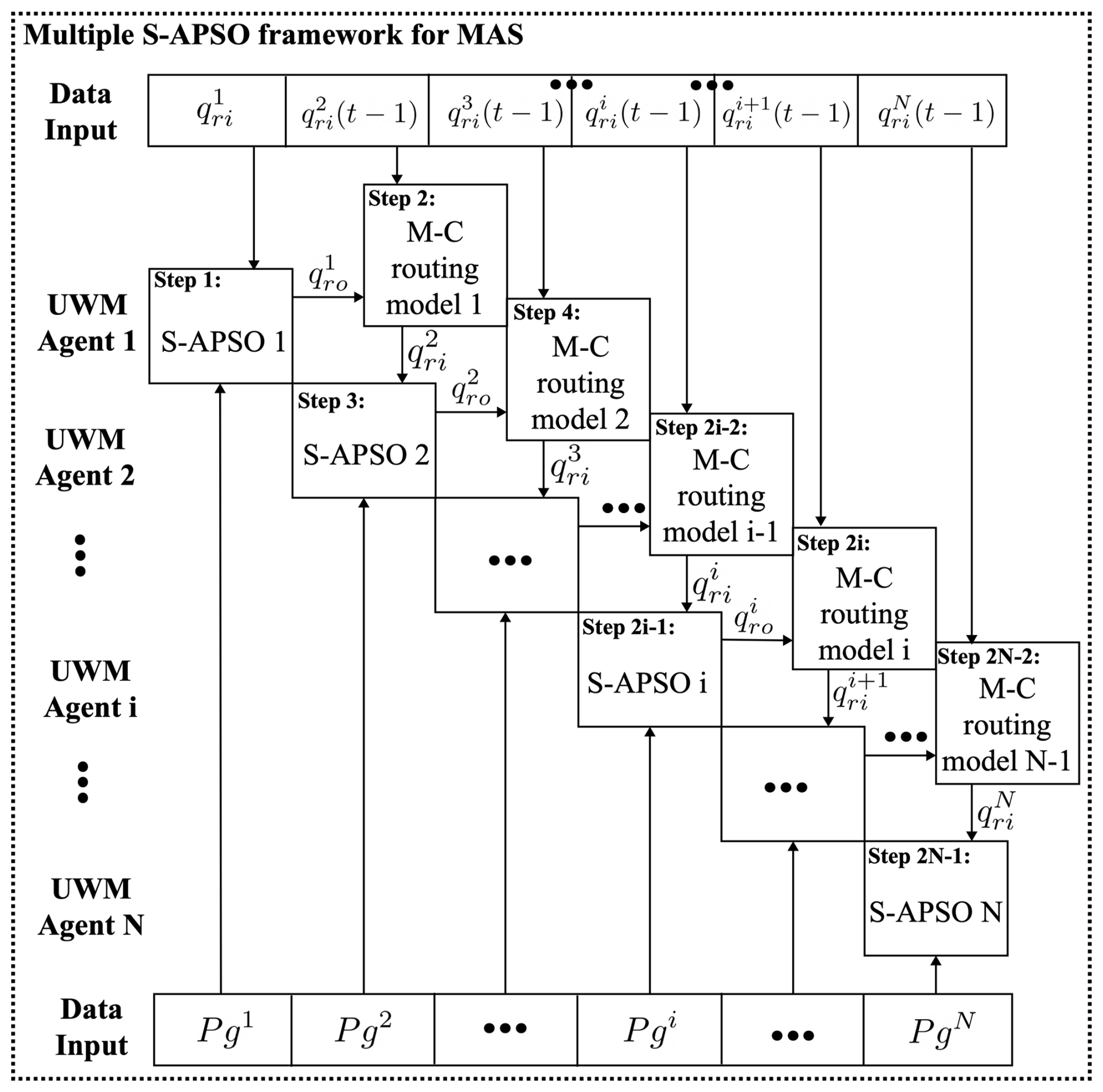
Figure E1 Flowchart diagram of the multi-S-APSO framework to multiagent system for inter-city-scale IGWM.

Appendix F: Details of the bi-level multiagent system for watershed-scale IGWM

This appendix presents a thorough and comprehensive examination of the bi-level multiagent system for IGWM at a watershed scale. The diverse components of the system are meticulously elucidated, encompassing elements such as the extended agent-based model for UWM, the bi-level multiagent system, and the pertinent solution approaches associated with this bi-level system.

F1 Extended agent-based model for UWM

Under the policy intervention from a WM, each UWM agent needs to make reasonable IGWM decisions to trade off the previous three types of costs (i.e., GI construction, water supply, wastewater drainage) and the possible penalty fee set by a WM to minimize their own total IGWM costs under the specified low streamflow thresholds. Therefore, the above UWM agent model will be extended – its annual IGWM cost function is converted as the sum of GI construction, water supply, wastewater drainage costs, and penalty fees. Taking the UWM agent i as an example, the extended agent-based model for UWM under the streamflow penalty strategy is shown as follows:

$$\begin{array}{}\text{(F1a)}& {\displaystyle }\underset{W,\mathrm{GI}}{min}{\mathrm{TC}}_i=C_{\mathrm{gi}}+C_{\mathrm{si}}+C_{\mathrm{wi}}+P_i\text{(F1b)}& {\displaystyle }\mathrm{s}.\mathrm{t}.\left\{\begin{array}{lr}{P}_i=\sum _{t=\mathrm{1}}^{\mathrm{12}}{r}_{\mathrm{p}}\cdot \left[\frac{\left[q_{\mathrm{ro}}^i\right(t)-S_q^i(t\left)\right]+\left|q_{\mathrm{ro}}^i\right(t)-S_q^i(t\left)\right|}{\mathrm{2}}\right];& \left(\mathrm{01}\right)\\ \mathrm{Eq}.\left(\mathrm{B}\mathrm{1}\mathrm{b}\right);& \left(\mathrm{02}\right)\\ q_{\mathrm{ro}}^i\left(t\right)=\mathrm{1000}\cdot A_{\mathrm{u}}^i\cdot \left[Q_{\mathrm{ro}}^i\right(t){]}_{*}.\forall t& \left(\mathrm{03}\right),\end{array}\right.\end{array}$$

where the first row of Eq. (F1b) indicates the annual penalty fee for the UWM agent i, and its calculation in detail shown as follows. The third row of Eq. (F1b) represents the units for hydrological parameters being converted from millimeters to cubic meters based on the associated urban total areas.

Penalty fees. In the extended UWM agent model, a penalty fee must be imposed on UWM agent when the outflow in its urban catchment is below the specified low streamflow threshold at the corresponding checkpoint. It is assumed that the WM prescribes a constant penalty rate for the watershed and that a penalty fee is only imposed on out-of-threshold streamflow. Hence, for UWM agent i in month t, if the outflow at checkpoint i is not below the low streamflow threshold (i.e., $q_{\mathrm{ro}}^i\left(t\right)\ge S_q^i\left(t\right)$), the penalty fee is 0; however, if it is below the quota (i.e., $q_{\mathrm{ro}}^i\left(t\right)<S_q^i\left(t\right)$), a fee equal to $r_{\mathrm{p}}\cdot \left[S_q^i\right(t)-q_{\mathrm{ro}}^i(t\left)\right]$ is imposed. By integrating the above cases, the annual penalty fee for UWM agent i can be written as

$$\begin{array}{}\text{(F2)}& P_i=\sum _{t=\mathrm{1}}^{\mathrm{12}}{r}_{\mathrm{p}}\cdot \left[{\displaystyle \frac{\left[q_{\mathrm{ro}}^i\right(t)-S_q^i(t\left)\right]+\left|q_{\mathrm{ro}}^i\right(t)-S_q^i(t\left)\right|}{\mathrm{2}}}\right].\end{array}$$

F2 Bi-level multiagent system

A streamflow penalty strategy prescribed by a WM agent might change some UWM agents' decisions of IGWM – upstream UWM agents might have to adjust their IGWM decisions to increase outflow to avoid over high penalty fees for costs minimization, which is beneficial to the downstream agents. Such changes in UWM agents' behavior can, to some extent, shift the interactions in the multiagent system for UWMs, which might have a potential impact on the watershed environment that can be measured by the assessment index (i.e., water allocation Gini coefficient) set by the MW (see Fig. 1c). Therefore, a WM agent can assess the effects of the policy on the watershed via checking the given index that reflects feedbacks of the multiagent system for UWMs and then gradually adjusts it to find the optimal one. This process is a WM–UWM agent interaction in watershed-scale IGWM under a water policy.

Fig. 1c illustrates that the WM–UWM agent interaction is no longer determined only by the WM or the UWMs, and both of them try to optimize their objectives (i.e., equity vs. cost objectives for WM and UWMs) under the associated constraints (i.e., streamflow vs. GI construction, water supply and demand constraints) and reactions of the other party. Therefore, they follow a specific decision rule. That is, the WM agent first makes a decision, and then each UWM agent specifies a decision to optimize their own objectives with full knowledge of the WM's decision; the WM also optimizes its own objective based on the rational UWMs' reactions. In economic theory, this process – the WM–UWM agent interaction – is a Stackelberg game (Von Stackelberg, 2010).

Therefore, the WM–UWM agent interaction can follow a hierarchical decision rule for the leader – the WM agent and the multiple followers – the UWM agents (Dempe, 2002). In addition, for the followers, the UWM agents form a multiagent system for UWMs (Eq. C10) that has a Markov property, which involves a special multi-stage decision-making process (Bellman, 1966). By integrating the WM (Eq. B4a), the UWM (Eq. F1) agent model, and the multiagent system for UWMs (Eq. C10) mentioned above, a bi-level multiagent system for WM–UWM agent interaction can be developed to describe the Stackelberg game between the WM and multiple UWM agents and unique multi-stage system constructed to reflect the state transitions for the multiple WM–UWM agents, which can be formulated as follows:

$$\begin{array}{}\text{(F3)}& \mathrm{Eq}.\left(\mathrm{B}\mathrm{4}\mathrm{a}\right)s.t.\left\{\begin{array}{l}\mathrm{Eq}.\left(\mathrm{B}\mathrm{4}\mathrm{b}\right);\\ \mathrm{where}{W}_i,{\mathrm{GI}}_i\mathrm{solves}\\ \left\{\begin{array}{ll}\mathrm{Eq}.\left(\mathrm{F}\mathrm{1}\right);& \forall i\\ \mathrm{Eq}.\left(\mathrm{C}\mathrm{10}\right);& \forall i,t\\ q_{\mathrm{ri}}^{\mathrm{1}}\left(t\right)=Q_t^{\mathrm{1}},\mathrm{and}{q}_{\mathrm{ri}}^i\left(\mathrm{0}\right)=Q_{\mathrm{0}}^i.& \forall i,t\end{array}\right.\end{array}\right.\end{array}$$

where $[-{]}_{*}$ represents the parameter being from the simulation calculation of the UWB-SM.

F3 Solution approach

In the bi-level multiagent system (Eq. 2), agent-based models for UWM are converted to Eq. (F1) due to the introduction of a streamflow penalty strategy. Compared with the above models (Eq. B1), only the objective function of the transformed model (Eq. F1a) is changed – adding a penalty fee. Therefore, to apply the proposed S-APSO to solve the agent-based models for UWM in the bi-level multiagent system, only the fitness function for particles needs to be adjusted. In addition, the above multi-S-APSO framework is also available in simulating the interactions among all UWM agents in the bi-level multiagent system under a given streamflow penalty strategy because of the features of its hydrologic connections – the Markovian property.

For the agent-based model for WM, the above S-APSO framework without the simulation-based initialization and the check and repair mechanism is available to look for the optimal solution due to its simple constraint conditions (Eq. B4ab). However, there is a critical factor in the simulation of the bi-level multiagent system that is how to deal with the special decision rule between the WM agent and the UWM agents – a Stackelberg game; i.e., the WM agent's best response is based on the associated reactions of all UWM agents (Von Stackelberg, 2010). In fact, it is challenging to obtain a Stackelberg solution to the bi-level multiagent system using general solution methods because the bi-level model is an NP-hard problem, even in its simplest linear case (Dempe, 2002). To deal with the specific bi-level model decision rules, the study nests the multi-S-APSO framework for the multiagent system for UWMs mentioned before into the particle performance measurement of the S-APSO for the WM, which can simulate the responses of the multiagent system for UWMs to a given streamflow penalty strategy prescribed by the WM agent, thereby assessing the policies' effects accurately. By the nested structure, therefore, a nested S-APSO framework is proposed for searching for the optimal WM–UWM interactions in the bi-level multiagent system under a streamflow penalty strategy. The flowchart diagram for the nested S-APSO is illustrated in Fig. F1.

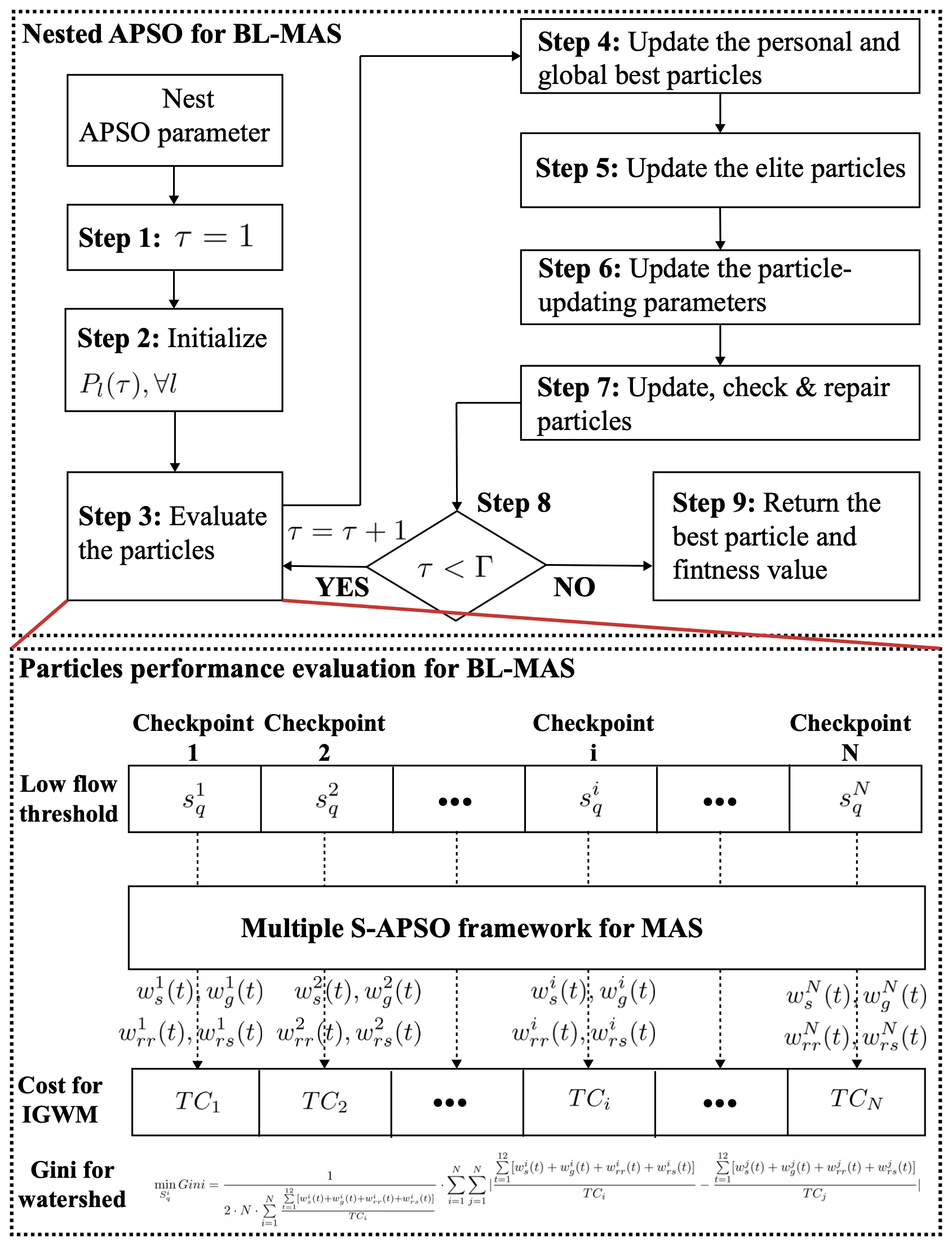
Figure F1 Flowchart diagram of the nested S-APSO framework to bi-level multiagent system for watershed-scale IGWM.