Technical note: High-frequency, multi-elemental stream water monitoring – experiences, feedbacks and suggestions from 7 years of running three French field laboratories (Riverlabs)

High-frequency and multi-elemental stream water monitoring are acknowledged as necessary to address data limitation in the fields of catchment sciences and freshwater biogeochemistry. In recent years, the development of stream bank analyzers and on-site field laboratories to measure various solutes and/or isotopes at sub-hourly measurement intervals has been in progress at an increasing number of sites. This trend should likely persist in the future as the technologies are still improving. Here we share our experiences of running three innovative lab-in-the-field prototypes, called Riverlabs, which consist of a field deployment involving continuous sampling and filtration of stream water and its analysis using laboratory instruments such as ion chromatographs. This note gives an overview of the technical and organizational points that we identify as critical because we claim that such practical considerations are generally missing in the literature in order to provide guidelines for the successful implementation of future projects running such or similar field-laboratory setups. We share the main stages in the deployment of this tool in the field, the difficulties encountered and the proposed solutions. Our two main conclusions for a successful, long-term functioning of these types of field laboratories are, first, the necessity to adapt several central components of the field laboratory to the local conditions (climate, river geometry, topography, physico-chemical characteristics of water, power supply) and, second, the need of diverse and in-depth technical skills within the engineering team. The critical aspects discussed here relate to (1) supply of the field laboratory – basic functioning of the pumping, filtration and analytical systems; (2) data quality control and assurance via maintenance services and operations; (3) data harmonization and coordination of the laboratory components; and (4) team structure, skills and organization. We believe that sharing these experiences, combined with providing some practical suggestions, might be useful for colleagues who are starting to deploy such or similar field laboratories. These considerations will save time, improve performance and ensure continuous field monitoring.

1 Introduction

Over the last 2 decades, monitoring of water quality parameters at high temporal frequencies has strongly developed based on various technologies (Kirchner et al., 2004; Wade et al., 2012; Rode et al., 2016; van Geer et al., 2016; Bieroza et al., 2023) with the motivation of advancing environmental sciences (Kirchner et al., 2004, 2023). Among these technologies, the emerging field laboratories, so far mainly used for surface waters, are running on the bank side of streams or rivers (Jordan and Cassidy, 2022). They often have more requirements than optical or other in-stream sensors in terms of filtration and power supply. They consist of running chemical analytical instruments in the field and relaxing the constraints of traveling for sample collection, sample storage, and the delay between sampling and analysis. For some solutes, field laboratories are the only possibility to measure their concentration in situ because no indirect method or proxy exists. Such technologies are associated with technical challenges that are related to the acceptable sample filtration, to the required level of maintenance and electrical power source (Bieroza et al., 2023). Jordan and Cassidy (2022) distinguished analyzers that are generally adapted from those used in the water utility or water treatment industries, from field laboratories developed specifically for the research sector. The latter include equipment of analytical laboratories such as laser spectrometers for isotope analysis (von Freyberg et al., 2017) or ionic chromatography for anion and cation analysis (Floury et al., 2017). Bieroza et al. (2023) identified six topics where significant advancements were achieved thanks to high-frequency water quality monitoring, and several studies demonstrated the importance of high-frequency concentration data for estimating the element loads exported from streams at annual or inter-annual scales (e.g., Cassidy and Jordan, 2011; Skeffington et al., 2015; Chappell et al., 2017; Wang et al., 2024).

However, to our knowledge, there is little literature from a technical and operational point of view, which can be used by the scientific communities that would like to design or run such analyzers. Nevertheless, improving the quality of high-frequency data sets was emphasized by Bieroza et al. (2023) as a critical issue, associated with the need for the development of robust protocols for maintenance and data management. Therefore, the objective of the present technical note is to provide guidance for running field laboratories, by detailing critical technical points and some suggestions successfully tested, in order to achieve continuous, reliable and usable data sets as soon as possible. The information presented in this technical note is derived from our experiences in managing three “Riverlabs” deployed in three French Critical Zone Observatories. These Riverlabs are prototypes of geochemical laboratories in the field developed within the CRITEX project, “Challenging equipments for the temporal and spatial exploration of the Critical Zone at the catchment scale” (Gaillardet et al., 2018), an instrumental program aiming at sharing innovative analytical facilities for French research in geosciences. The practical applications of such prototypes are to acquire water concentration data across a whole diversity of hydrological conditions (storm and base flow, high versus low flows) with the highest accuracy possible and for various elements, here all the major ions. This variety aimed at enabling analysis combining geogenic and anthropogenic elements with reactive versus conservative behaviors. It has to be noted that a new version of the Riverlab was manufactured and installed along the Sangamon River in Monticello (Upper Sangamon River Basin US Critical Zone Observatory), Illinois, USA, in July 2021. This Riverlab has been designed to be deployed along a river draining a 1500 km² catchment (Wang et al., 2024), much larger than the three catchments presented here. Some of the technical issues in this technical note have been solved in this new version, and some are likely to be scale specific and therefore different between the CRITEX Riverlabs and the Monticello cases. Therefore, here, from the comparison of the three contrasted observatories, we derived some critical points particularly relevant for a deployment in diverse headwater catchment conditions.

The note is structured into four parts: the water supply and filtration (Sect. 3); the interactions between the components (Sect. 4), including general components (Sect. 4.1) and measurement technologies (Sect. 4.2); the maintenance (Sect. 5), including internal maintenance (Sect. 5.1) and that provided by suppliers or manufacturers (Sect. 5.2) with associated frequencies; and, finally, the organization of running the Riverlabs (Sect. 6). We first illustrate issues encountered and then present the solutions developed.

2 Material and methods

2.1 Study sites

Three French sites which were equipped with a Riverlab (Endress + Hauser, France), are all part of Long-term Critical Zone Observatories (OZCAR-RI), distributed from western to eastern France (Fig. S1 in the Supplement). The Avenelles catchment was equipped with a first version of the prototype in 2015, whereas the Strengbach and Naizin catchments were equipped with a second version of the prototype in 2017. We describe the three sites from west to east briefly.

The Naizin catchment (AgrHyS Observatory, Fovet et al., 2018) covers 5 km² in central Brittany. The elevation ranges from 98–140 m above sea level (m a.s.l.), and slopes are gentle (<5 % on average). The bedrock is composed of upper Proterozoic schists. The rather impervious unaltered bedrock is overlain by a fractured zone, where water can percolate, and by a weathered layer, 1–30 m deep, where shallow groundwater can fluctuate. The climate is temperate and humid with an average rainfall of 837 mm and an average temperature of 11.2 °C. The soils are silty loams, between 0.5 and 1.5 m deep, and well drained except in bottomlands close to the streams. Land use is dominated by agriculture (91 %), with cereal crops (maize, straw cereals) and grasslands. The stream dries out almost every summer for a period of up to 4 months.

The Avenelles catchment is a 45 km² sub-catchment of the Orgeval experimental catchment (ORACLE Observatory, Tallec et al., 2013) located 70 km east of Paris. Its elevation ranges from 85–130 m a.s.l. and the topography is relatively flat. The geological context corresponds to a multi-layer aquifer system with two sedimentary tertiary formations: the shallower Brie aquifer (Oligocene limestone) that is separated by a discontinuous grey clay layer (Priabonian mudstone and Bartonian marl) from the deeper Champigny aquifer (Eocene limestone). The climate is semi-oceanic, average annual rainfall is 740 mm and mean annual air temperature is 9.7 °C. Deep loamy soils are highly homogenous and usually tile-drained (80 % of the agricultural lands). Land use is dominated by agriculture (82 %), with cereal crops (wheat, maize, barley and pea).

The Strengbach catchment (OHGE observatory, Pierret et al., 2018, 2019) is a 0.8 km² granitic watershed located in the Vosges Mountains. Its elevation ranges from 880–1150 m a.s.l. with heavily incised side slopes (mean slope of 15°). The bedrock is mainly composed of Hercynian Ca-poor granite (315±7 Myr), which was subjected to hydrothermal alterations of various levels with main hydrothermal alterations occurring 183.9 Myr ago (El Gh'mari, 1995). The thickness of the granite arena varies from 1–9 m. The local climate is temperate oceanic mountainous with a mean annual temperature of 6 °C. Average annual precipitation is 1380 mm, with snowfall occurring 2–4 months per year. The soils are brown acidic to ochreous podzolic series and are generally about 1 m thick. Land use is dominated by forests (85 %), composed mainly of spruces (80 %) and beeches (20 %).

2.2 Riverlab prototypes

The three French Riverlabs have a similar design and similar functioning (Fig. 1; for further details about the first Riverlab, see Floury et al., 2017). The Riverlabs are organized into three main parts, namely the pumping system, the filtration system, and analytical instruments and sensors, which are all housed in a container-like shelter. Hereafter, we describe the design and functioning of these three French Riverlabs. Note that in the US prototype, the specific setup designed for the Sangamon River station is described in the supplement of Wang et al. (2024).

Figure 1 Diagrams of the three CRITEX Riverlab prototypes.

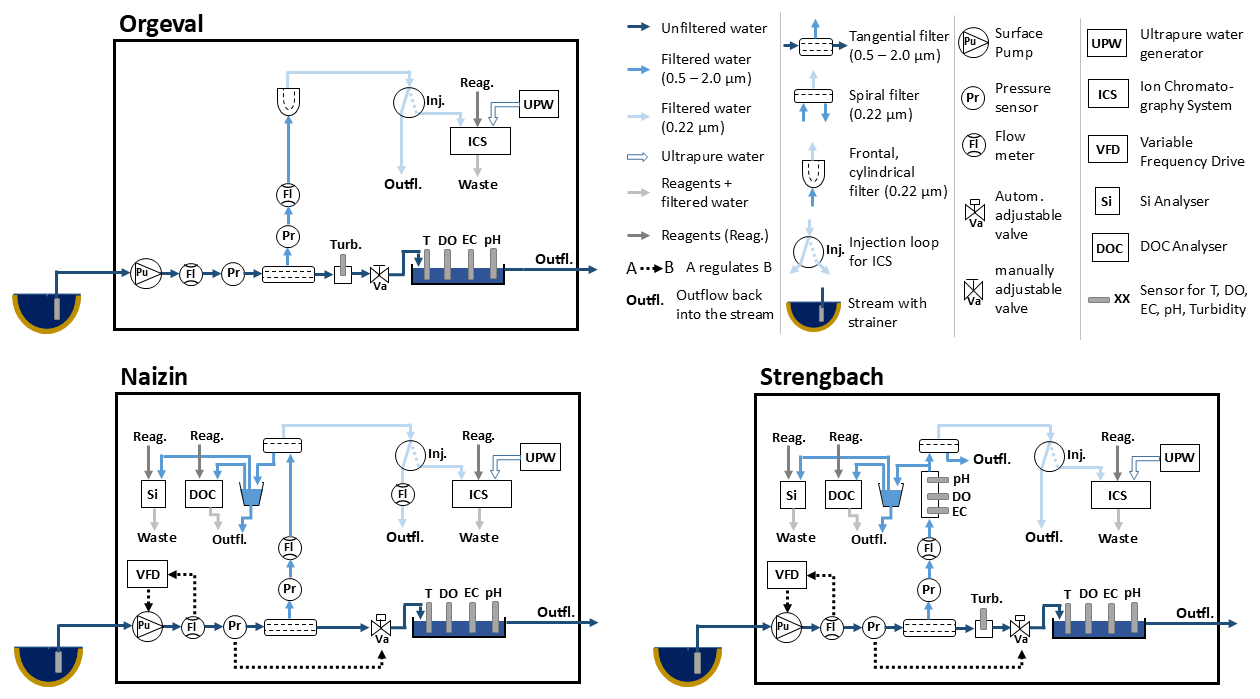
A surface pump (Wilo, WJ-203-X-DM-IE3 or Grundfos, JP-5-B-A-CVBP-E-N or PCM Moineau modèle 2M6F Cycle 25.4 cm³ 1000 rpm), located inside the Riverlab, provides a continuous flow of unfiltered stream water, with a regulated, constant flow and pressure. The stream water is aspired through a strainer in the stream (variable sizes and configurations for the different Riverlabs, for example, ISCO-type strainer at Strengbach) and pumped through a hose (inner diameter ∼2 cm; length of around 5 m at Naizin and Orgeval and 141 m at Strengbach) into the Riverlab at a flow rate of 500–1300 L h⁻¹. As a substitute or to increase the power of the surface pump, a submersible pump (Calpeda, borehole pump, type: 4CS 0,55T – 4SDX 1-9) was tested at Naizin and Orgeval for a short period (see Sect. 3.1.1).

Inside the Riverlab and downstream of the pump, the unfiltered water flows through flow and pressure sensors, a tangential filter, an adjustable pressure valve, and an overflow tank with sensors for physico-chemical parameters. Sensor probes monitored temperature (Thermophant T TTR31, Endress + Hauser), electrical conductivity (EC, Condumax CLS21D, Endress + Hauser), dissolved oxygen (DO, Oxymax COS61D, Endress + Hauser) and pH (Orbisint CPS11D, Endress + Hauser) at a 1 min time step. At the Strengbach and Orgeval catchments, the unfiltered water also flows through a turbidity sensor (Turbimax CUS52D, Endress + Hauser). The regulation of the flow and the pressure of the unfiltered water are achieved manually at the Orgeval Riverlab, whereas at the other two sites this is done automatically with a PID (proportional integral derivative) controller. The controller is continuously adjusting the aperture of the adjustable valve and the pump speed (via a variable-frequency drive) depending on the differences between the measured and targeted water pressure and flow, respectively.

The filtration system is composed of two parts. In the first part, the unfiltered, pressured stream water flows through a tangential, stainless steel filter (pore size of 0.5–2 µm, depending on the site), which continuously produces filtered stream water (with a flow rate between 10 and 15 L h⁻¹ at Strengbach and 1.5 L h⁻¹ at Naizin, not measured at Orgeval). Accordingly, the pressure drop across the first filtration step by the tangential filter is smaller at Naizin (around 0.5 bar, from 1.8–1.3 bar) than at Strengbach (around 1 bar, from 2.0–1.0 bar) and at Orgeval (around 1.4 bar, from 2.0–1.0 bar). This first tangential filter is cleaned automatically every few minutes (ultrasonication and reverse flow) and, additionally, manually every few weeks. At Strengbach and Naizin, around two-thirds of this filtered water flows through a second set of DO, EC and pH sensors (at Strengbach only) and is used for further analysis in other instruments (LAR QuickTOCuv from Anael for dissolved organic carbon (DOC) and Stamolys CA71SI from Endress + Hauser for dissolved Si). A small part (a few percent or less) is filtered through a second spiral cellulose acetate filter (diameter of 47 mm and pore size of 0.22 µm) in a spiral tangential filter setup (Strengbach and Naizin) or in a frontal cylindrical filter setup (Orgeval) to provide filtered water to the ion chromatography system (ICS5000+ from ThermoFisher Scientific). At Naizin, the flow after the second filtration step (0.22µm) varied between 0.03 and 0.18 L h⁻¹ (Fig. 4), while at Orgeval it was close to 1 L h⁻¹ (not measured at Strengbach). This second filter is replaced manually every week to fortnight.

All analytical instruments (ICS, DOC analyzer, Si analyzer) and sensors (DO, EC, pH, turbidity) are regularly checked for drift, cleaned and calibrated. The chemicals and pure water that are required for the analyses by the instruments are regularly prepared in the university or research center facilities and subsequently delivered to the Riverlab. The effluents and liquid wastes produced by the instruments are either ejected back into the stream, if they are of no environmental concern, or collected in containers and subsequently returned to the laboratories for appropriate processing.

In the following sections (Sects. 3–6), we present some of the challenges encountered, the solutions applied, and some practical guidance for future users of this or similarly complex field laboratories.

3 Water supply of the field laboratory

3.1 Stable supply of unfiltered stream water during storm events and variable hydrological conditions

During (high) rainfall events, water level, turbidity and particle concentrations increase in the watercourses, sometimes by several orders of magnitude (Cotel et al., 2020; Vongvixay et al., 2018; Lefrançois et al., 2007). The variations can be very rapid, especially in very small headwater systems or during events such as flash floods. In general, these events can lead to an increased presence of bubbles and vortexes in the stream. Moreover, in temperate catchments, the autumn season is associated with a flushing of tree leaves, branches and other clogging material that can block the opening of the strainer. All these disturbances can reduce the stability of the pumped flow delivered to the field laboratory and likely affect the residence time of the water in the water circuits.

3.1.1 The supply of unfiltered water

We identified four major aspects which may induce or prevent potential failures of the pumping system. These are (a) the choice between a surface or submersible pump; (b) the design of the strainers, baffles and the intake hose; (c) the combination of the pump and the variable frequency drive (Supplement); and (d) the appropriate regulation of the pump by the PID controller.

Regarding the pump type, all three Riverlabs were initially equipped with a surface pump. For around 5 months, at Naizin we tested (5 km²) a submersible pump that does not need to be primed. However, at Naizin and Strengbach, surface pumps almost never lost their prime even if they were stopped and re-started remotely, while at Orgeval, this was a recurrent issue. The submersible pump occupied an important portion of the stream cross-section even at Naizin and Strengbach where the stream is small. We tried to prevent inhalation of debris with baffles and strainers. However, deposition of fine organic and mineral particles into the submersible pump led to strong wear and tear after a few months (Fig. S2 in the Supplement).

During storm events and independent of the pump type, the pump was frequently not able to supply the targeted water flow value to the Riverlab (Fig. 2). Due to this issue, the strainers and baffles required a re-design to be well adapted to the local conditions and avoid their clogging during storm events. At Naizin and Orgeval, with important inputs of large broadleaves and branches in autumn, the initial strainer was too small and therefore frequently clogged by a few leaves during the first autumn storms. The adaptation of the strainer eventually consisted of a small strainer with a small pore size nested within a larger strainer with larger pores, which has been working well since. At Strengbach, in contrast, the initial setup was too large for the cross-section of the stream and therefore accumulated debris during storm events but, at the same time, had too few and too small pores. A cylindrical ISCO-type strainer was then used, which was additionally equipped with an easily removable mesh around it. After several trials, a mesh size of 2 mm was chosen and has been working successfully since (Fig. 3).

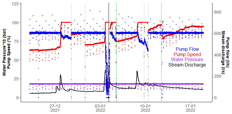
Figure 2 Pump flow (blue, L h⁻¹), pump speed (red, %), water pressure (purple, bar) and stream discharge (black, L s⁻¹) at the Naizin catchment. A submersible pump was used: grey bars indicate manual pump stops and re-starts, green bars indicate pump cleaning, and black bars indicate an automatic pump stop due to instabilities. Note the periods of full pump speed (100 %) during the storm events, when the targeted flow values are not reached, and the decreasing pump efficiency (red; increased pump speed necessary for a given flow) over the course of those 4 weeks.

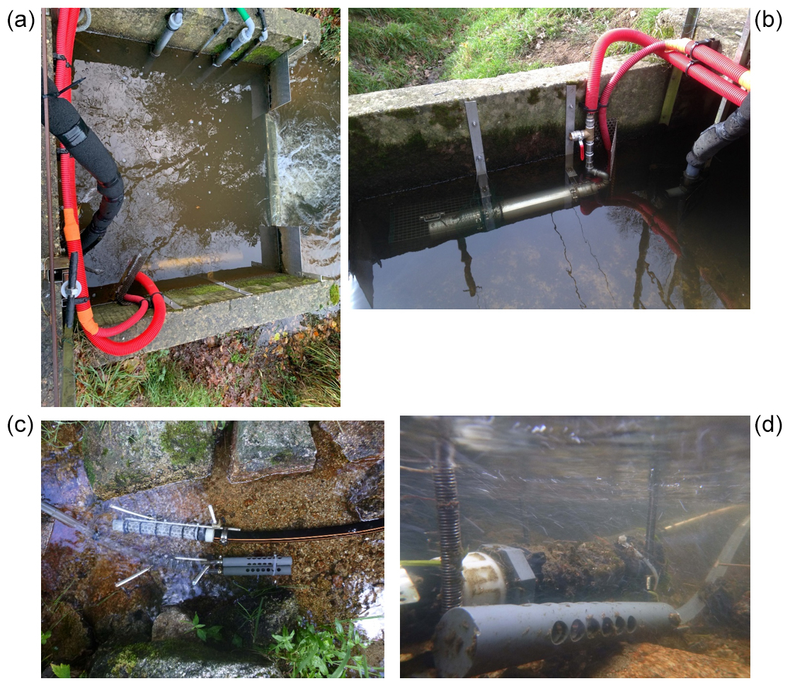
Figure 3 Pictures of the strainers and baffles in the Naizin (a, b) and Strengbach (c, d) stations to prevent clogging of the pumps.

Finally, the PID controllers can be adjusted by tuning some parameters to optimize the response to a deviation of the measured flow and pressure of the unfiltered water from its target values. In order to avoid instabilities, we set a relatively fast adjustment of the flow controller and a slow adjustment of the pressure controller. In addition, both adjustment times need to be slower than instabilities especially high during storm events. It is inadequate to have a fast-reacting PID controller that is trying to adapt to the instabilities of the system. The parameters of the PID controller need to be established empirically on a case-by-case basis.

3.1.2 Tips and good practices

Following the main challenges concerning the pumping system, here we provide some guidance for a successful design of this system and some potential points of attention. From our experience, an individual adaptation of the pumping and strainer system to the local conditions is paramount. For this local adaptation, important characteristics to consider are turbulence and sediment transport capacity of the stream, particle size distribution of the suspended sediments, input of organic debris, and stream width and depth, as well as maximum and minimum water temperature (risk of freezing). In hindsight, we acknowledge that a submersible lifting pump might have been more adequate than a submersible borehole pump to handle fine organic and mineral particles. However, lifting pumps often require a deeper stream than borehole pumps and are therefore not the best option in small streams.

Commercially available and adapted or hand-made strainers in addition with baffles or deflectors are necessary in order to prevent the clogging and the wear of the pump. However, there is no one-fits-all design of the strainers. The pore size of the strainer needs to be large enough to allow the provision of a maximum flow, and at the same time, it needs to be small enough for protecting the pump and filtration system from too much debris and sediment. We advise conducting some tests locally with different pore sizes in different hydrological and turbidity conditions. Finally, the strainers should not be too close to the streambed in order to avoid the influx of bedload particles.

The type and number of intended analyses and their analytical requirements in terms of water volume (for the analysis and the turn-over of the water volumes) might also impact the required flow and, therefore, the choice of the pump. Additionally, the altitude difference between the field laboratory and the water intake needs to be considered when choosing the pump type, as explained above. At Orgeval and Naizin, the water intake is a few meters below the field laboratory, while at Strengbach, a long hose between the strainer and the Riverlab is responsible for an inverse gradient, where the water intake is above the field laboratory. In that latter case, the challenge is less to prevent pump failures but more to conduct maintenance of the long hose.

Finally, it is very advisable to have remote access to the field laboratory and its main components with the possibility of re-starting the pumping system remotely.

3.2 Stable supply of filtered stream water

The filtration of water before analysis usually meets two different objectives. One is related to the scientific questions and interpretations of the analyses when one targets the quantification of dissolved phases of some constituents. This is the case, for instance, for the dissolved forms of some nutrients (P, N, Si) expected to be more bioavailable. Another motivation for filtering is to prevent the clogging of the circuit and the wear of the analytical equipment. However, filtration might influence the analysis when involving large volume of filtered water (Horowitz et al., 1992). Finally, when designing the on-line filtration system, a trade-off needs to be found between the risk of filter clogging (due to a high flow through the filter) and the risk of a long residence time in the circuits (due to a low flow through the filter).

3.2.1 Critical aspects and challenges of the filtration system

Filtration of the water requires a compromise between the addition and management of a filtration unit and the preservation of analytical units. As an example, in the initial design of the Riverlabs, the carbon analysis (total organic carbon concentration) was carried out on the unfiltered water. However, during high-flow periods, we observed fast fouling of the tubing and the analytical equipment, which would have required a monthly or even bi-weekly cleaning or replacement of the entire tubing system. Therefore, we decided to analyze the DOC concentration on water filtered at 0.5 µm to preserve the analyzer and to avoid clogging of the tubing.

First, the spiral filter with a surface area of only 17.3 cm² (the area used for the actual filtration is much smaller) tends to clog at a rate that depends on the hydrological condition and on the size of the suspended solids in the stream. During floods, when the water is turbid, the flow passing through the 0.22 µm filter decreases very quickly, up to 83 % within a week (Fig. 4). This has a significant impact on the residence time of the water within the circuits that is not constant over time. It therefore leads to asynchronies between the different analytical equipment depending on whether they are supplied with 0.22 µm filtered water or not (Fig. 5). We will detail this point regarding possible asynchrony between different instruments in Sect. 4.3. In addition to the organic and mineral material coming directly from the stream, particles and biofilm can accumulate in the tubing of the circuits and can be remobilized later during cleaning sequences or surges of water flows (e.g., when replacing the 0.5 µm filter). Hence, regular replacement or cleaning of as much plumbing as possible is required, especially through parts that form angles and that cannot be easily disassembled (e.g., the housing of the oxygen probe in the filtered water circuit, Strengbach Riverlab).

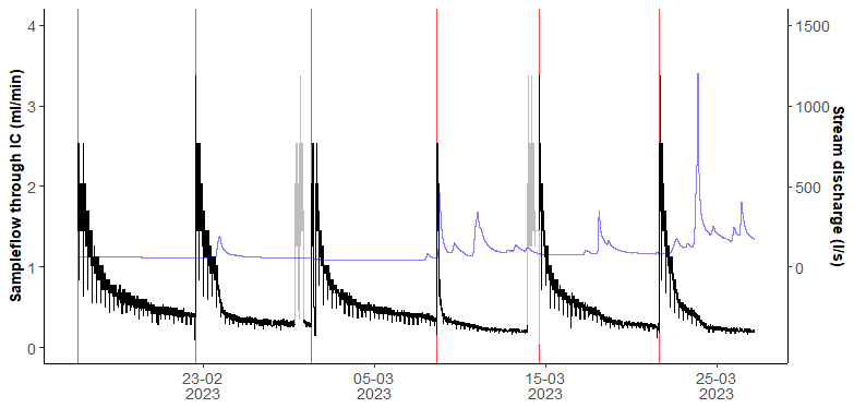
Figure 4 Evolution of the flow at the output of the ionic chromatograph (IC) in black and stream discharge in blue, at the Naizin catchment. Red bars indicate a change of the spiral filter (0.22 µm), and grey periods are due to purging of the IC with ultra-pure water.

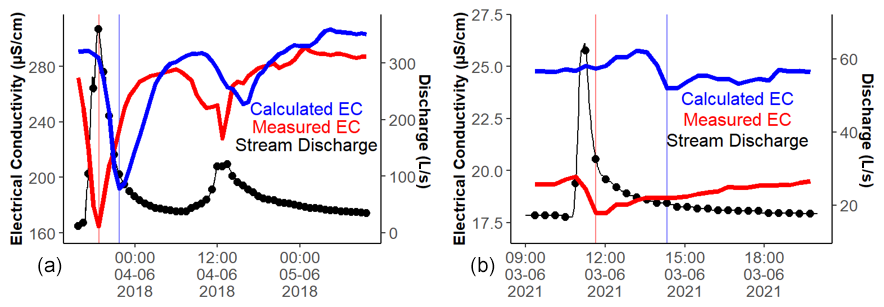
Figure 5 Estimation of the transit time between the overflow tank and the ion chromatography system (IC) at the Naizin (a) and Strengbach (b) catchments. The transit time was calculated as the difference between the measured electrical conductivity in the overflow tank (red) and the calculated electrical conductivity computed from ion concentrations measured in the IC. The black dots along the hydrograph (black line) indicated the moments when a water sample was injected into the IC, and the red and blue vertical bars indicate the timing of the minimum measured and calculated electrical conductivities, respectively. The time difference between these two bars amounts to 2 h 54 min at Naizin (a) and to 2 h 41 min at Strengbach (b) and can be used as a proxy for the transit time. The long transit time is primarily due to the clogging of the second filter (0.22 µm).

This clogging had a direct effect on the analytical results of certain elements, particularly sulfate. ICS-analyzed sulfate concentrations tend to decrease during filter clogging (up to 30 % at Naizin during 1 week, Fig. 6). Lab analyses of samples taken from the circuit before and after the spiral 0.22 µm filter indicated that the filter acted as a sink of sulfate. The removal of sulfate increased over time and with the clogging state of the filter (Fig. 6). This issue of the sulfate measurement was not observed with the frontal cellulose acetate 0.22 µm filter at Orgeval, where sulfate concentrations are also 1 order of magnitude higher than in the two other streams.

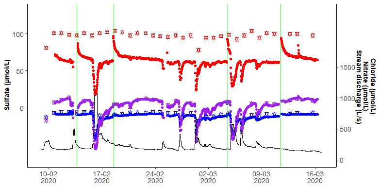
Figure 6 Evolution of the sulfate (red), chloride (blue) and nitrate (purple) concentrations and stream discharge (black) measured in the Riverlab at the Naizin catchment; green bars indicate a change of the spiral filter (0.22 µm). The points are concentrations measured in the Riverlab, whereas the stars are concentrations measured independently in our lab from daily grab samples from the stream.

Finally, we also identified a contamination in cation analyses on the three Riverlabs. Indeed, significant concentrations of Ca, Mg and K have been measured with the ICS in Milli-Q water samples that did not contain these elements when verified in the lab (ICP-MS verification). Such contamination developed gradually over time (Fig. 7) and can disturb the validation of the calibration curves, with low points affected by this contamination. The ICS had to be flushed with many Milli-Q water samples in order to achieve a sufficiently low level of background concentration.

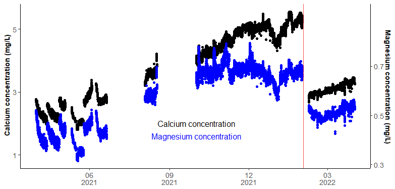
Figure 7 A long-term and gradual contamination issue was observed in the three sites affecting cation analyses, specifically calcium and magnesium, illustrated here for Strengbach. According to our investigation, this issue is likely occurring either in the PEEK tubing used between the 0.22 µm filter and the ionic chromatography system which are several times longer than the tubing usually used in the laboratory or in the injection loops. The vertical red bar indicates the date when the injection loop of the cations was changed.

In Strengbach, the gradual increase in the calcium (+250 % in a month), magnesium (+180 % in a month) and nitrate (+125 % in a month) concentrations was confirmed when analyzing certified material (a lake water with a chemical signature similar to that of the Strengbach River) every 2 weeks, showing that these elements adsorb to or are released by the tubing material. A similar effect was observed in the other two Riverlabs but to a lesser extent, likely due to the higher background ion concentrations.

3.2.2 Interpretations and solutions

The various tests carried out showed that the sulfates were adsorbed on the paper filter or on the particles retained on the filter, since the sulfate concentration analyzed at various points in the filtered water line only decreases at the outlet of the 0.22 µm filter. Changing the filter material from cellulose acetate to nylon (conducted at Naizin during several weeks) did not solve the problem in terms of both the decrease in flow (clogging) and the loss of sulfate. The decrease in sulfate concentration is all the more visible as the concentration in this element is low. A decrease of 3 mg L⁻¹ by the filter represents around 30 % in Naizin, while in Orgeval, this decrease was likely not noticed because the background sulfate concentration is much higher (70 mg L⁻¹), and the particle load to the filter is less important. In addition, the nature of the solid suspended matter retained on the filter is different depending on the geology of the sites and on the land use of the catchments. Finally, we closed the bypass circuit of this spiral acetate 0.22 µm filter (that is, we forced all the water through the filter), and the sulfate issue was almost completely solved.

Regular cleaning of all the PEEK tubing, including the injection loops, as recommended by ThermoFisher Scientific with acetonitrile$/$water (1$/$9) and HCl (1N) solutions, respectively, followed by rinsing with Milli-Q water helps to reduce the contamination and to find an acceptable background concentration of the blank. The other alternative is to change the PEEK tubing regularly. Although PEEK offers very high chemical resistance to many elements, base acids or solvents, our observations suggest that over time this material can, under certain conditions, gradually adsorb certain elements and release them during the passage of corrosive solutions such as ultra-pure water or standard solutions made with Milli-Q water. It is crucial that any change or cleaning on the tubing preceding the injection loop requires a new calibration of the instrument and the analysis of certified material to be sure that the subsequent injections will be analyzed accurately. In Strengbach, the injection loop and the tubing segments are changed at least every month or when a suppressor/column change is made, and a new calibration of anions and cations is performed after stabilization of the signals. Contrary to Strengbach, in the Naizin and Orgeval Riverlabs, we only noticed a slight (Naizin) or no (Orgeval) long-term contamination of the measurements of stream water. This might be due to the higher cation concentrations in the latter two catchments.

4 Data harmonization and coordination of the laboratory's components

The field laboratory is composed of many different analyzers and sensors with different measurement and acquisition time steps. Therefore, the time series measured by the different instruments have to be synchronized before data analysis, which is not always straightforward. The exploration of synchrony between concentrations or any other parameter measured in the Riverlabs and the stream flow needs to be performed cautiously. In addition, some sensors interfered with other equipment in the Riverlab. It is, therefore, critical to be aware of potential interferences between different components of the Riverlabs and to assess the synchrony or asynchrony of the acquisition by the different sensors and analytical instruments.

4.1 Connectivity and interferences between the different devices

An example of an unexpected interference was observed between an uninterruptible power supply (UPS) and differential circuit breakers. Almost the entire Riverlab is connected to an UPS system. Furthermore, the whole electrical circuit is protected by differential circuit breakers to protect the people working in the Riverlab. However, specific differential circuit breakers are required that are on the one hand sensitive enough to protect the people and on the other hand robust enough (i.e., accepting very short surcharges) to cope with an UPS. The initial installation did not consider these aspects, resulting in sporadic and irregular power outages. Identifying the causes of these power outages was a major challenge for the local team as well as for the external equipment providers due to this unusual configuration.

Furthermore, we encountered frequent, but irregular, disconnection errors of the ICS. Various modules of the ICS (e.g., dual pump, eluent generator, chromatography module) are connected to a central computer with USB cables. Initially, we used standard USB cables and a USB hub. Following the repeated disconnection errors of some of the modules, we replaced the hub by an internal USB expansion card and the standard USB cables by shielded cables. These replacements solved our disconnections errors. Additional unexpected interferences (e.g., the impact of the ventilation system on the water level measurements) are listed in the Supplement.

4.2 Choice of analytical and sensor technologies

The choice of the analytical and sensor technologies in the Riverlab has consequences for the exploitation of the acquired data. This choice depends on (i) the precision and stability of the available technologies; (ii) its suitability to the local chemical conditions of water, especially the ranges of values; and (iii) the consistency between instruments and their respective water sampling strategy.

• i.

  Precision and stability of the technology. This is related to the compromise between the direct uses of laboratory instruments in contrast to analytical instruments that are specifically designed for field operations. The latter might have a lower quantification performance but also a lower reagent consumption and waste production, as well as a better robustness. In addition, the long-term, continuous operation can have impacts on the performance of classical laboratory instruments that were not designed for this continuous operation. This was the case of the long-term drifts of the calcium and magnesium concentrations likely linked to the PEEK tubes of the ICS. For regular use, lab-based, non-continuous measurements, the PEEK tubing might be adequate, but an alternative material in continuously operating field laboratories might be useful.

• ii.

  Suitability to the local chemical conditions. The sensor technologies, analytical instruments and analytical protocols, including the calibration and the controls with certified standards, need to be adapted to the local conditions and requirements as well. For instance, at Orgeval, calcite precipitation occurred in the tubing and instruments (ICS) as well as in the overflow tank and on the sensors. Frequent cleaning and purging with acid or the replacement of the tubes was necessary there. In contrast, at Strengbach, the low ion concentrations were likely responsible for the faster wear of the pH sensor, which required frequent replacement.

• iii.

  Consistency between instruments. In catchments with a fast-changing water chemistry, it might be important to consider the differences in the way water is supplied to the different instruments to facilitate the process of synchronization of the acquired data. At Naizin and Strengbach, the DOC analyzer in the Riverlabs, for example, continuously extracts filtered water from a small overflow tank. In addition, the DOC analyzer itself contains a reaction tube, which is replenished continuously. Its quasi-continuous measurements are an integration over several minutes to tens of minutes. This is in contrast to the ICS, where discrete measurements are based on the injection of a small sample volume at a precise and short moment of time. In addition, a variable and unequal transfer time from the stream to these different instruments adds another source of inconsistency. Therefore, combining these different types of data needs to be performed carefully with checking of the synchrony between measurements.

4.3 Data management and dedicated software

Instrument manufacturers often develop commercial software for managing the data acquired using the instruments they supply. The different software can more or less manage import of data acquired from other instruments, but the importation of the additional data is possible to automatize to a certain extent. In the French Riverlab cases, ion concentration data from ICS analyses have to be processed using the Chromeleon™ software (Thermo Scientific), whereas all other variables are centralized to a data manager and logger RSG45 (and RSG40 for Orgeval in a first phase, Endress + Hauser). These data can be visualized and exported using ReadWin software and later the Field Data Management software (both Endress + Hauser) with specifiable parameters. Text files downloaded from these different interfaces can also be uploaded into classical software used for data exploration and analysis such as R, Python or MATLAB. The Extralab company also developed a software solution with automatic import of text files produced by the ICS and of the text files from the logger and tools for visualizing the time series, tools for data request design, and application for programming the exploration and analysis of the data using notebooks. In the configuration of the French Riverlabs, the critical step was the ICS processing using the Chromeleon™ software because it requires a check of the quality of the chromatograph and of its numerical integration and possibly adjustments (e.g., of retention times) by an analyst expert. This critical step could be addressed using two strategies. One strategy would be to develop algorithms for expertizing the chemical analysis with the manufacturers of analytical instruments and going a step further in the automation of data analysis and controls and security tools. Another strategy would be to develop a data processing chain that takes into account, adapts to and valorizes the expertise of chemical analysts. Such a processing chain should include standardized (i.e. associated with norms) facilities to describe expert actions and possibly corrections in the processed data sets.

4.4 Solutions and perspectives for synchronization

Automation of the data qualification can be partially achieved using variables related to the system states (pressure of filtered water, pump speed, etc). For instance, the solution proposed by the Extralab company (“Protocol” function available in the ExtraLab^® Dashboard, https://www.extralab-system.com/product, last access: 6 June 2024; Paris, France) was to create filters for excluding data corresponding to a pump speed value that deviates too far from the target which have to be specified by the operators.

For synchronizing the different concentration data as well as the hydrological and physico-chemical parameters, several non-exclusive options are possible. At Naizin, for example, temperature and/or conductivity measured by sensors in the overflow tank was also measured directly in the stream, next to the strainer, using a similar sensor technology, which enabled us to quantify and correct the delay between both signals. At Naizin, constant-rate injections of salt solutions at low flow (6.7 L s⁻¹) allowed us to quantify this delay between those two EC sensors as ca. 8 min. A similar delay was computed at Strengbach and in Orgeval; Floury et al. (2017) estimated this delay to be ca. 5 min. The same injection allowed us to estimate that the delay between the stream and the ICS can reach up to 30–40 min at this low flow value and when the 0.22 µm cellulose acetate filter was 1 week old (Fig. 8). Estimates of this delay can also be approximated by computing the theoretical conductivity based on the ion concentrations from the ICS and to compare it to the electrical conductivity measured with the sensor in the overflow tank or in the stream (Fig. 5). This method works especially well if the EC measurements vary considerably during a storm event. In contrast, this method cannot be used during small storm events, which do not lead to a clear variation of the EC signal (as we observed at Strengbach). Alternatively, the outflow of the ICS could be measured continuously and could be correlated with measurements to quantify this time lag. Salt injections could be used to measure the time lags between the intake of the water at the strainer and the arrival at the ICS, at various degrees of the filter clogging. These measurements could then be used to establish a correlation between the time lag and the measured outflow of the ICS.

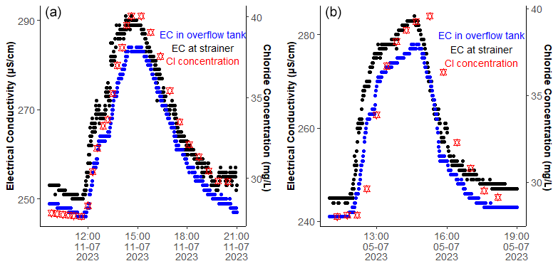
Figure 8 Salt tracer test for the determination of the travel time within the Riverlab at Naizin with a clean (a) and a 1-week-old (b) 0.22 µm spiral filter. For both injections, a salt solution was injected continuously 123 m upstream of the strainer for a period of around 70 min. The electrical conductivity was measured by a hand-held EC meter next to the strainer (black) and in the overflow tank (blue). The chloride concentrations were measured by the ICS with manually shortened run times (15/20 min instead of 35 min). During both injections, the travel time between the strainer and the overflow tank was around 10 min. However, the travel time between the strainer and the ICS was around 10 min with a new filter (a) and around 35 min with an old filter (b).

Once these delays are estimated, one option might be to average and homogenize the data time series rather than using the instantaneous ones, for example for the ion and carbon concentrations, pH, EC, DO, temperature, and stream water level. An hourly average, for instance, would still be sufficient to study dial variations and storm flow variations in Naizin and Orgeval. It would be too coarse for storm flow variations in Strengbach though. Instead of a continuous filtration, another alternative in the system design for insuring synchronization would be to filter only a small, sampled volume of water at 0.22 µm at specific and known moments of time, as is done in the Swiss field laboratory (von Freyberg et al., 2017). This choice minimizes the clogging and the degradation of the filter but requires an additional sampling step.

5 Data quality control and insurance by regular maintenance

As any classical laboratory, the Riverlabs need a quality control procedure and regular maintenance to allow the exploitation of reliable data and metadata. This section reviews the main categories of the maintenance operations that we concluded to be mandatory in our cases, in order to help future potential users to design and anticipate this maintenance part. Even if some detailed operations will vary depending on the specific settings of the field laboratories (the choice of the equipment, the station's configurations, etc.), we believe that this list might serve as a valuable point of departure to estimate the costs and skills required for running any field laboratory. As an order of magnitude, the operating costs were between EUR 10 000 and 20 000 per year per Riverlab in 2018–2022.

5.1 Annual to weekly maintenance operations and strategies

5.1.1 Major maintenance categories and frequencies

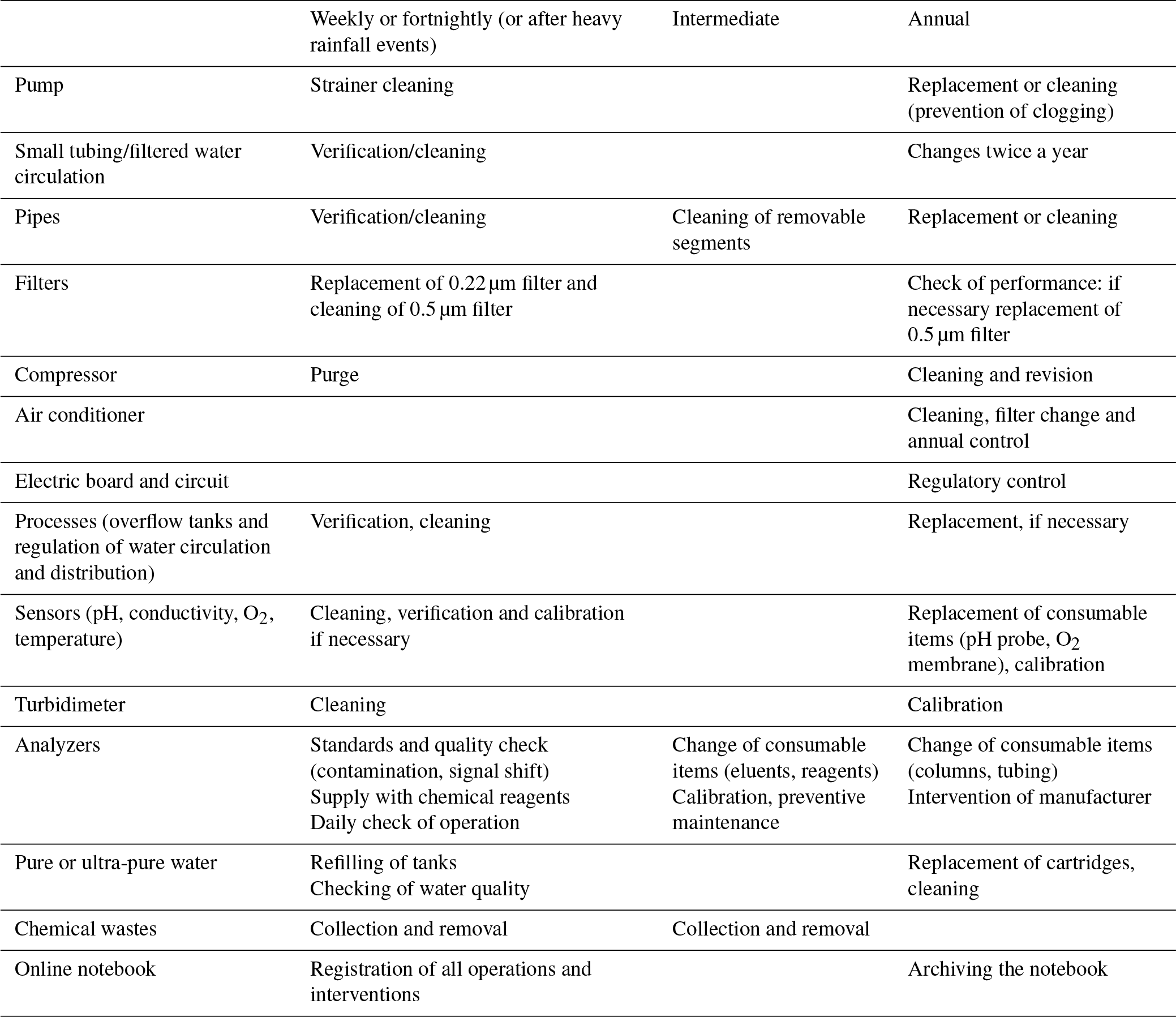
The three Riverlabs are located between 80 and 100 km from their reference research centers. The technical staff performs maintenance operations on site every week (Naizin) or every 2 weeks (Strengbach, Orgeval). The Riverlabs require very regular maintenance, including cleaning of tubing, pipes, tanks and sensors; calibration of probes and analytical tools; replacement of filters and consumables (e.g., eluent cartridges, columns, reagents); reparations of various failures, removal of chemical waste; and quality control using certified standards, as well as purging of the air compressor (Table 1). For these regular maintenance operations, interventions every week or every 2 weeks seem to be sufficient, in our experience. However, additional and spontaneous interventions might be required for solving some problems quickly (pump failures, power outages, measurement drift, contaminations, etc.), and occasional breakdowns require timely on-site interventions (pump breakdowns, electrical problems, breakdowns in measuring equipment, leaks, etc.). For these sporadic instances, local inhabitants were trained to conduct basic interventions, for which they were compensated for. The budget necessary for running a Riverlab has two aspects: the routine and the unexpected reparations. The budget for the routine includes various expenses and is as complex as an analytical laboratory because of the large number of service providers. The budget for the repairs of large breakdowns is more difficult to plan, especially because the Riverlabs are exposed to a variety of meteorological conditions as well as to human and animal activities. These repairs included expensive parts of the analytical and technical equipment due to multi-year wear, lightning strikes, or other factors.

Table 1 List of maintenance operations for each component of the Riverlab, with an indication of the frequency of each operation.

5.1.2 Possible alternative strategies for simplifying water supply and chemical waste management

In an early stage of the development phase of the Riverlabs, in the Orgeval observatory, ultra-pure water for the ICS was produced on-site directly from stream water instead of bringing demineralized water to the field for supplying ultra-pure water. However, due to very fast saturation and clogging of the on-site ultra-pure water production system, it was replaced by a routine, where demineralized water from the laboratories was frequently transported to the Riverlabs. In this updated version of the Riverlab, the demineralized water was stored and subsequently purified by a Millipore system for eluent production and regular purging, which consumed on average around 1 L d⁻¹. Since the containers for storing the demineralized water are relatively large (in total 20 L at Naizin, 30 L at Strengbach, only 10 L at Orgeval), they only need to be replenished every 2–3 weeks (every 10–15 d at Orgeval), which is less frequent than the regular interval at which the Riverlabs are visited. As a side note, the Riverlab at Strengbach ran without a Millipore system for several years, without any worsening of the analytical quality, which reduced the running costs. Ultra-pure water (18.2 MΩ) was transported to and stored in the Riverlab and was directly used by the ICS.

In addition to the provision of the reagents for the different analytical instruments, it is very important to consider the handling of the produced chemical waste from these instruments (solvents, reagents etc.). Two aspects are important here: the potential environmental hazard of the waste concentration and its produced volume. For the first case, we evaluated whether the residual concentrations of the reagents in the waste might reach concentrations that could be of environmental concern, especially during low-flow periods. We concluded that the ejection of the waste coming from the DOC analyzer back into the stream was of no concern. In contrast, the waste of the ICS had to be collected. The volume of the produced waste by the ICS (6 L per week at highest analysis frequency) is relatively small and can therefore be easily handled, by returning it frequently to the lab. This is in contrast to the Si analyzer, which is producing up to 35 L of waste per week at the highest sampling frequency (every 20 min). We therefore had to reduce the sampling frequency of the Si analyzer in order to be able to manage its produced waste. This example illustrates the importance of considering the waste production during the selection procedure of the different analytical instruments because a low waste production is not always targeted when manufacturers and suppliers develop new instruments.

5.2 Support and maintenance by manufacturers and suppliers

The Riverlabs' running depends on the correct functioning of many different technical and analytical components, which were provided by separate suppliers. Due to this unique combination of the different components and the problems arising from their interaction, the individual suppliers were not aware of those problems and their causes and frequently pointed at components of other suppliers. This made some failures very complex and difficult to solve and required a competent technical team with detailed knowledge of the Riverlab. As an example, at Strengbach, we hypothesized that the air compressor contaminated the pressurized air, which is needed for the DOC analyzer. Therefore, the analyzer produced erroneous measurements. Another example is the biased water level measurements caused by the ventilation system of the Riverlab at Naizin that are described in the Supplement.

For analytical instruments, such as the ICS, we opted to have a maintenance contract with the supplier, as it allowed us to receive quick and detailed feedback and, therefore, to solve unknown problems more swiftly. This comes, however, with an elevated cost (EUR 7700 per year in 2016). In addition, maintenance costs can be reduced elsewhere. At Strengbach, for example, cartridges of one of the eluents were regularly prepared in the laboratory from a concentrated solution and were not acquired in a ready-to-use concentration from the supplier. This required some additional preparation time but reduced the cost for the eluent by a factor of almost 50.

5.3 Consequences for the management of measured time series

Producing long time series of concentration data so that they are easily accessible and usable often requires a mix of manual and automatic quality control procedures. Riverlab data management thus includes several challenges, as highlighted for various high-frequency water quality monitoring facilities (Cassidy and Jordan, 2022). We identified three main challenges associated with data management (Fig. 9). In our experience, a detailed, technical knowledge of the effect of the different components and their interactions on the measurements is required.

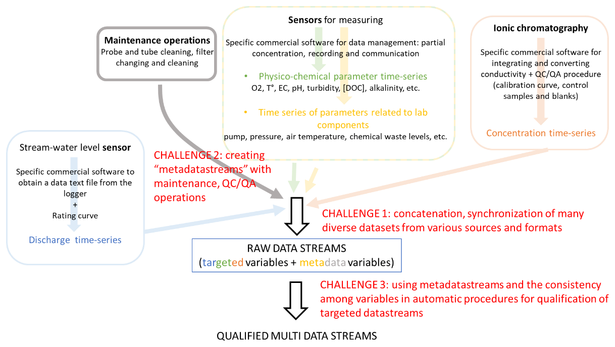
Figure 9 Data management workflow of the CRITEX Riverlabs and associated challenges. QC/QA: quality control/quality assurance. O2: dissolved oxygen concentration. T°: water temperature (in °C). EC: electrical conductivity in water. [DOC]: dissolved organic carbon concentration.

Data validation of the ion concentration time series from the ICS is conducted regularly and manually by technical members of staff, who were maintaining it and who were, therefore, aware of any relevant malfunctions or inaccuracies of the system. This allows us to directly and undoubtedly remove non-validated measurements from the concentration time series.

The first challenge (Fig. 9) is therefore related to compilation of the various data sets, especially if sensors and technologies need to be synchronized (e.g., time lags, injection versus continuous flow analysis). In other cases, specific routines in the functioning of the Riverlab had impacts on certain measurements during finite periods. It required detailed technical knowledge in order to interpret these additional variations correctly. For example, a programmed flushing of the whole pumping cycle artificially increased and decreased the temperature in the overflow tank slightly during the flushing. This rapid temperature variation in turn influenced the temperature-corrected electrical conductivity due to a lag of the temperature adaptation of the conductivity sensor.

Interventions in the Riverlab, such as maintenance work, modifications and repairs, were recorded in electronic (and sometimes paper) logbooks, which all project participants could share and access. Depending on the noting system, these interventions were, however, not directly linked with the database, nor were they in a tabular format. Because this information had to be extracted manually from the logbooks, it was not possible to visualize the logbook data, such as the days when a specific filter was replaced, in a concentration time series. In addition, due to the multitude of the work conducted during a single field day at the Riverlab, an individual log entry often contained information about many different activities. It was therefore challenging to identify from the logbooks when specific parameters of the functioning of the Riverlab had changed during previous interventions. The second challenge (Fig. 9) is therefore to convert the information in the logbooks into data streams (called “metadatastreams” in Fig. 9), i.e. time series of interventions (such as filter change, pump cleaning, standard sample analysis). The third challenge (Fig. 9) is thus related to translating this technical knowledge into algorithms that will use non-targeted monitored variables (e.g., room temperature, pressures, pump speed and velocity) to curate and qualify the monitored variables targeted (e.g., water temperature, pH, conductivity and concentrations). Finally, the database must be collected and archived with all relevant metadata.

6 Team structure, skills and organization

To run field laboratories over the medium to long term (from several years to decades), it is necessary to dedicate available and competent scientific and technical resources to ensure its proper functioning and the collection, analysis and archiving of a large quantity of data. Even if the number of work hours required to produce these large number of analytical results is drastically reduced by these field laboratories, the need for human resources remains important. The combination of skills required to run such a field laboratory is also new and highly diverse. In this section, we aim at highlighting the organizational challenges associated with such technological innovations and try to give recommendations to avoid neglecting these challenges.

6.1 Team organization

The organization of the Riverlab team members is mainly based on their skills and coordination, as many operations are dependent on each other. The optimum functioning of the Riverlab requires multiple and varied skills in the field of analytical chemistry, sensor installation and calibration, electronics, hydraulics and others. All tasks and implications for each team member should be clearly discussed and formalized. Due to their remote location, it is necessary to establish good communication and organization of interventions on the Riverlab, with an archive of the history of all operations. For this purpose, an online notebook, accessible both in the Riverlab and in the offices and laboratories, is a well-adapted tool. Furthermore, a precise intervention schedule, elaborated and shared between the different actors, is necessary.

The Riverlab requires interactions with many manufacturers, subcontractors and service providers. It is therefore necessary to have an up-to-date directory of contacts with the technical relays but also the commercial ones of these various structures.

6.2 Team skills

Field laboratories require therefore various and complementary skills. Obviously, as is the case for any analytical laboratory, it requires technical skills in chemical analysis, especially to run and control the data from the ICS. Technical skills in field instruments for environmental monitoring are also essential to understand and to properly conduct the maintenance of the various sensors. As highlighted in Sect. 3, the supply of water to the analyzers and instruments is also critical in the running of the Riverlab, and this requires skills related to the functioning of the pumping and filtration systems. As any laboratory, the field laboratory also requires the application of rules related to health and safety, the periodic inspection of the electrical installations, etc. In addition, the remote nature of such field laboratories, and their purpose to produce high-temporal-resolution data, requires skills in remote communication systems and in data management (information systems, databases, etc.). Synchronization issues, data curation, archiving and traceability of these processes require computer-assisted protocols and therefore corresponding software skills. Finally, good communication and organizational skills are crucial regarding the amount of consumables and equipment and the number of contact persons.

In the case of the three French Riverlabs, the strategy of sharing different expertise and skills in a team appeared to be successful and key in solving technical issues, especially in this testing phase of the prototypes, but required, again, strong communication skills. Sharing the maintenance of the Riverlab between several people was also necessary in order to continuously operate the field laboratories, which can includes on-call duty for weekends and holidays. Organization skills are therefore necessary for sharing the work and the information and for using appropriated tools (e.g., shared calendar).

7 Conclusion

Scientific perspectives in the fields of hydrology, geochemistry, aquatic ecology and environmental geosciences have been suddenly and highly renewed with the development of field laboratories and other technologies enabling near-continuous measurement of water quality. The acquisition of funding for equipment and material has to be synchronized with funding for running the equipment and for covering the human costs associated with such infrastructures that involve many challenges, both technical and organizational.

In this technical note, we reviewed the critical aspects we experienced in the testing phase of three field laboratories for measuring in situ and at sub-hourly frequency the major element concentrations in stream waters. One of the main conclusions from our cross-experiences is that a very large number of components and parameters needs to be adapted empirically to the local conditions. This type of complex field laboratory is not a one-fits-all system that can be deployed anywhere without significant adjustments, and in our experience a settling period of 2 to 3 years was necessary, but, thanks to recent improvements, this period tends to be much shorter. We highly recommend paying close attention to the first tests when hydrometeorological conditions are changing, ideally with the possibility of making adjustments with the manufacturer. Furthermore, a non-negligible amount of diverse and detailed knowledge and human resources is paramount for the acquisition of reliable data. Specific technological skills are required to operate such a tool in the fields of hydraulics, filtration, electricity, sensor maintenance, electronics, telecommunication, data treatment and data management. In addition, it is essential to validate data before they can be processed and interpreted. We believe that the critical steps identified here, and the solutions we recommend, can be transposed beyond our specific equipment from those tested by our three teams. This technical note is a practical guide to help design the project of running these or similar field laboratories and then to acquire original and precise data sets as fast as possible. Promising results have already come out of these experiences (Floury et al., 2017, 2024; Tonqui-Neira et al., 2020a; 2020b; 2021; Brekenfeld et al., 2024, accepted; Wang et al., 2024), and more will come. Several issues have been solved, and some issues we experienced did not occur in the US deployment (Wang et al., 2024) where the instrumented station drained a larger area and was characterized by higher volume and fluxes of water. High-frequency geochemical data can be used to study processes in several disciplines (hydrology, biogeochemical cycles, ecology, microbiology, agronomy, etc.) and on several timescales (dial, event, seasonal, annual, etc.), with many avenues still to be explored.