Cold climates, complex hydrology: can a land surface model accurately simulate deep percolation?

Cold regions present unique challenges for land surface models in simulating deep percolation or potential groundwater recharge. Previous model evaluation efforts often overlooked these regions and did not account for various sources of uncertainties influencing model performance. This study uses high-resolution integrated lysimeter measurements to comprehensively assess the performance of the Soil, Vegetation, and Snow (SVS) land surface model in a cold climate. SVS performs well in the daily snow depth simulation, with a correlation coefficient (r) greater than 0.94 and a mean bias error (MBE) smaller than 3.0 cm for most of the simulation period. The newly implemented soil-freezing scheme simulates the near-surface soil temperature reasonably well (r: 0.89), with a slight cold bias (MBE: −0.8 °C). However, the results show that SVS is limited in matching the temporal dynamics of deep percolation (daily timescale). In addition, it significantly underestimates deep percolation (r: 0.35, MBE: −0.8 mm d⁻¹) and near-surface soil moisture (MBE: −0.058 m³ m⁻³) during cold months. This is likely to be related to the model's inability to represent frozen-soil infiltration and preferential flow. These limitations must be addressed to make SVS a reliable tool for simulating deep percolation in cold environments. The findings highlight the importance of a comprehensive model evaluation to identify key deficiencies and to guide future model development efforts to improve hydrological simulations in cold regions. Such improvements lead to more informed decision-making regarding groundwater resource management in a changing climate.

1 Introduction

Groundwater is a vital resource facing increasing pressure worldwide, with declining recharge rates threatening its sustainability (Noori et al., 2023; Wada et al., 2010; Gleeson et al., 2012; Dalin et al., 2017; Nygren et al., 2021). Recharge is mainly driven by the deep-percolation process (Cao et al., 2016; Gurdak and Roe, 2010; Bakker et al., 2013; Ghasemizade et al., 2015), which refers to the net downward flux of water below the root zone (Bethune et al., 2008; Selle et al., 2011). Understanding and accurately estimating deep percolation poses a significant challenge for hydrologists (Blöschl et al., 2019). This challenge increases substantially in cold regions (Kurylyk et al., 2014), where the movement of water on the land surface is influenced by processes such as soil freezing and thawing (Iwata et al., 2010), snowmelt and accumulation dynamics (Harpold and Molotch, 2015), and rain-on-snow (ROS) events (Mazurkiewicz et al., 2008; Trubilowicz and Moore, 2017). These processes can substantially affect the timing and magnitude of deep percolation and groundwater recharge. For example, soil freezing and thawing cycles can change soil structure and permeability (Chamberlain et al., 1990; Chamberlain and Gow, 1979). Frozen soil can significantly affect water partitioning at the surface by impeding water infiltration and creating an impermeable layer (Li et al., 2021; Al-Houri et al., 2009). This is particularly consequential during snowmelt periods where the influx of meltwater mainly leads to surface runoff rather than to deep percolation (Iwata et al., 2018). Macropores within the frozen-soil layer during thawing can serve as preferential flow pathways and allow water to bypass the frozen matrix and reach the underlying unfrozen soil (Watanabe and Kugisaki, 2017; Sammartino et al., 2015). This preferential flow facilitates infiltration. Additionally, it significantly influences the hydraulic and thermal properties of the frozen soil by altering water and heat transport (Watanabe and Kugisaki, 2017; Walvoord and Kurylyk, 2016; Shirazi et al., 2009).

Despite the aforementioned challenges, accurate estimation of deep percolation remains a critical priority in cold regions. This is particularly crucial given that climate change is driving shifts in precipitation patterns (Trenberth, 2011; Dore, 2005) and snowmelt dynamics (Yang et al., 2022; Musselman et al., 2017), which, in turn, can impact groundwater recharge (Al Atawneh et al., 2021). Therefore, accurate modeling of deep percolation is essential for simulating the effects of climate change on water availability, which informs sustainable water management strategies in cold regions. Physics-based numerical (hydrological) models, such as land surface models (LSMs), are valuable tools for understanding and modeling deep percolation. Atmospheric scientists originally developed LSMs to address the limitations in early general circulation models (GCMs) that used fixed boundary conditions for land surfaces and failed to capture the complex interactions between the atmosphere and the land surface (Fisher and Koven, 2020). Manabe (1969) developed one of the first-generation LSMs to simulate these interactions using a simple “bucket” model for representing soil moisture. This model simplified land surface processes by focusing on the top meter of soil, where precipitation instantly infiltrated, evapotranspiration was the only way water left the soil, and runoff occurred when the soil became saturated (Yang, 2004). Subsequent generations of LSMs, such as Noah (Niu et al., 2011), and ISBA (Decharme and Douville, 2006), recognized the need for more realistic representations of vegetation and soil, which have a crucial role in the exchange of water and energy at the land surface. These complex models can explore hypothetical scenarios, enhance our understanding of physical processes, and provide explanatory, process-based predictions (Willcox et al., 2021). For example, they help quantify how changing precipitation patterns impact groundwater recharge (Taylor et al., 2013; Green et al., 2011; Wu et al., 2020). This is particularly important in regions where fluctuations in groundwater resources heavily influence ecosystem water availability (Huang et al., 2019; Orellana et al., 2012). Beyond natural systems, LSMs can guide the design of landfill final covers. By simulating the interaction of prospective covers with local hydrometeorological conditions (Ho et al., 2004), designers can optimize these covers to minimize leachate production, thereby saving time and resources.

Considering the complexities of cold regions and potential model limitations (Pomeroy et al., 2022), a key question relates to whether these models can accurately simulate deep percolation and its response to climate change. This is particularly crucial in cold environments with intricately linked water and energy fluxes (Wheater et al., 2022; Cordeiro et al., 2017). This necessitates a rigorous evaluation. Robust process-based model evaluation is integral to assessing the LSMs' “fits for purpose” (Beven and Young, 2013) and to identifying areas for targeted improvement (Wilson et al., 2021). A point-scale evaluation, in contrast to larger-scale evaluations, may allow for a detailed assessment of the model's ability to capture hydrological processes in cold environments by reducing the uncertainty in model parameters and meteorological data. This approach has been successfully employed in similar studies (Zhang et al., 2016; Denager et al., 2023; Chadburn et al., 2015). Evaluating deep-percolation simulations necessitates not only assessing the final output but also examining how well an LSM represents the key physical processes influencing it. Several factors complicate such evaluations.

First, direct measurements of deep percolation by lysimeters are difficult, costly, and scarce (Li and Shao, 2014). Lysimeters are containers or vessels, like a soil column, filled with soil or other material. They come in various forms, such as weighing (Payero and Irmak, 2008) or non-weighing pan lysimeters. Pan or zero-tension lysimeters are large-scale and are typically used for measuring percolation over a relatively large area. Pan lysimeters that are carefully designed can account for the spatial variability of the soil and the presence of preferential flow pathways and can resolve percolation rates as low as 0.1 mm yr⁻¹ (Malusis and Benson, 2006). While indirect methods, such as those using soil water content data, are critically limited in accounting for deep percolation due to preferential flow (Khire et al., 1997; Benson et al., 2001), lysimeters minimize errors substantially and can be used to calibrate the indirect methods (Benson et al., 2001; Meissner et al., 2008; Ouédraogo et al., 2022).

Second, pinpointing limitations in models' structures and parameterizations requires accounting for uncertainties in forcing data and parameter values (Oreskes et al., 1994). Finally, choosing an appropriate temporal resolution for model evaluation is crucial. High-resolution observations, such as those obtainable from lysimeters at daily or hourly time steps, help identify the strengths and weaknesses of how specific processes are represented in such a model. Coarse-resolution (annual or total) evaluation may hide compensating errors in simulating different processes. We performed a literature search (Scopus) to assess previous model evaluation studies that compared simulated deep percolation with lysimeter measurements. The search yielded 57 articles published between 1998 and 2024. Figure 1c represents the locations of these case studies on the map. Figure 1a and b provide the frequency of climate types (Köppen classification; Peel et al., 2007) and evaluation timescales, respectively. Our survey shows that about 60 % of the studies evaluated models' deep percolation at coarser-than-daily resolutions. HYDRUS (Simunek et al., 2005) was the most common model (28 out of 57), followed by UNSAT-H (Fayer, 2000). Only two LSMs were evaluated: ISBA (Sobaga et al., 2023) and HTSVS (Mölders et al., 2003). A key finding relates to the lack of attention to strategies accounting for different sources of uncertainty. None of the studies accounted for the uncertainty in forcing data and observations, and only four accounted for parameter uncertainty (Schwemmle and Weiler, 2024; Selim et al., 2023; Graham et al., 2018; Ogorzalek et al., 2008). This is an important limitation, particularly in the context of cold regions, because small biases in forcing data can significantly impact process simulations (Wheater et al., 2022). Snow and soil-freezing processes were rarely considered (only one study analyzed their influence, namely Mölders et al., 2003). The limited consideration of snow processes is likely to be due to two factors: the geographical distribution of case studies and model limitations. The case studies are concentrated in temperate (58 %) and arid (24 %) regions, with a smaller representation in continental zones (15 %), indicating a focus on areas where snow is less prevalent. Additionally, model limitations in some instances necessitated the removal of snowy periods from the analysis (Vásquez et al., 2015) or simplification of approaches like a degree-day snowmelt constant (Stumpp et al., 2012).

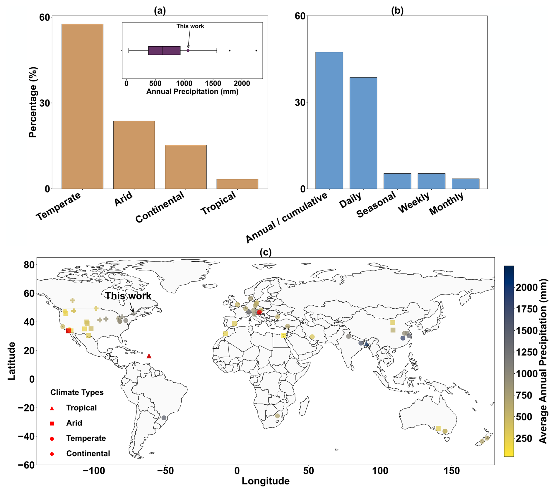
Figure 1 (a) Distribution of Köppen climate types across the case studies within the reviewed works, showing the percentage of studies for each climate type. The inset boxplot displays the average annual precipitation range across all studies. (b) Percentage frequency of temporal resolutions used for evaluating deep-percolation model outputs in the reviewed literature. (c) Global distribution of case study locations from the reviewed literature, categorized by Köppen climate classification and color coded by average annual precipitation. Triangles indicate locations where precipitation data were missing and obtained from an alternative source.

This study comprehensively evaluates the Soil, Vegetation, and Snow (SVS, Alavi et al., 2016; Husain et al., 2016) LSM in a cold environment setting. Environment and Climate Change Canada (ECCC) developed and operationally uses SVS for hydrological forecasting (Gaborit et al., 2017). By addressing the identified shortcomings in previous model evaluation efforts, we evaluated SVS's ability to simulate deep percolation using high-resolution data from a large, experimentally constructed plot (soil enclosure) in southeastern Quebec, Canada. The plot was equipped with two pan lysimeters and a network of soil moisture and soil temperature sensors. We used an ensemble simulation strategy, accounting for uncertainties in forcing data and (a subset of) the model's soil hydraulic parameters. Our assessment explicitly accounted for uncertainties due to measurement errors and soil heterogeneity. The uncertainties were factored into the calculation of performance metrics. Additionally, we implemented a simple soil-freezing scheme, which is assessed for the first time in the scientific literature for SVS.

2 Case study

2.1 Experimental plots

Figure 2b indicates the location of the experimental plot within the St-Nicéphore landfill site (“study site”) in Drummondville, Quebec, Canada. An aerial view of the plot post-construction is provided in Fig. 2a. The plot was fully covered with grass 1 month after construction. Two lysimeters were constructed in 2018 within the same enclosure shown in Fig. 2a. The top and bottom of the excavation followed the regulatory requirement of a 2 % slope. The soil configuration and the dimensions of the pan lysimeters, namely the L1 and L2 lysimeters, are illustrated in Fig. 2c. The 4 m × 4 m lysimeters were lined with a 1.5 mm thick HDPE geomembrane mounted on a wooden frame. A 100 mm thick gravel layer was included at the bottom of the lysimeters, overlaid by a 100 mm sand layer. The gravel layer served as drainage, while the sand layer acted as a filter to prevent clogging by the cover material (both shown in Fig. 2c). The lysimeters differ only in terms of height: L1 is 2.10 m high, while L2 is 1.50 m. The comparison between L1 and L2 is the subject of Kahale et al. (2022), where it was demonstrated that the L2 lysimeter collected nearly the same amount of percolation as L1 (less than 5 % difference). The lysimeters measured deep percolation hourly using tipping counters (KIPP-100, METER Group Inc.; 100 mL per tip). Soil water content and temperature were monitored half-hourly by dielectric sensors (METER Group Inc., 5TM), represented by blue dots in Fig. 2c, until October 2021. After this date, the data loggers were used in another project, and soil data collection stopped. However, percolation measurements continued until October 2022. Despite designing and constructing two surface water (runoff) collection systems, neither yielded reliable measurements and so were excluded from the model evaluation. Soil matric potential sensors were also installed at various depths in the plot but are not shown in Fig. 2c because they were not used in the analyses. Figure 2c shows the 15 cm topsoil layer atop the cover material (a sandy to silty soil commonly used as final cover at this landfill site). Table 1 outlines the properties of the topsoil and cover material. We used sieve and hydrometer analyses to determine sand and clay content. The soil's (vertical) saturated hydraulic conductivity (k_sat) was obtained using KSAT and Mini Disk Infiltrometer (Naik et al., 2019) devices (METER Group, Inc.). The soil water retention (SWR) model's empirical parameters, namely the air entry suction and the slope of the SWR curve (ψ_ae and b), were derived in the laboratory using the HYPROP (METER Group, Inc.) technique proposed by Schindler and Müller (2017); Schindler et al. (2015). The SWR curves for the topsoil and cover material are presented in Fig. 3.

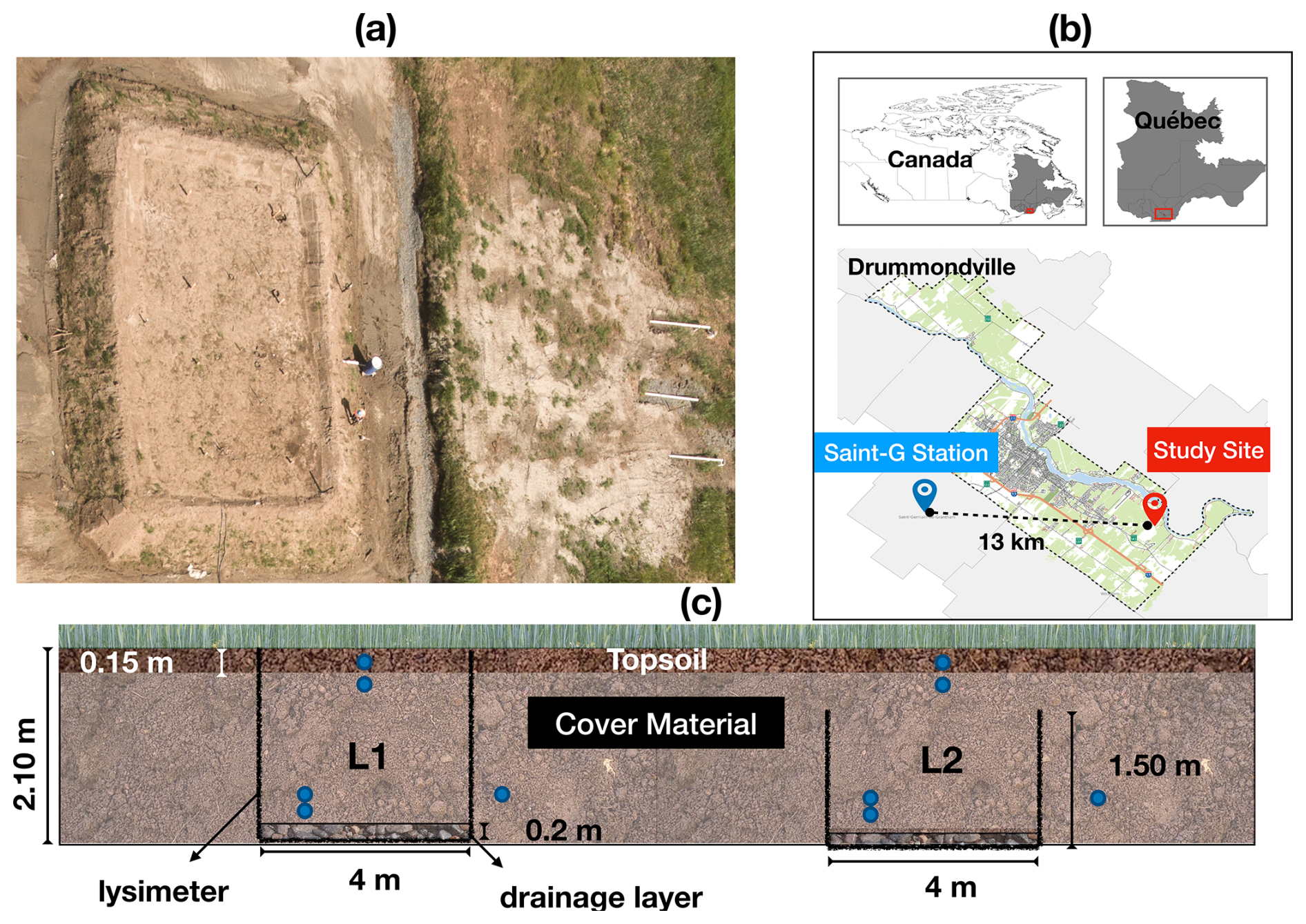
Figure 2 Experimental setup at the St-Nicéphore landfill. (a) Aerial view of the experimental plot at completion. (b) The location of the experimental plot (red marker) and the Saint-Germain-de-Grantham (Saint-G) weather station (blue marker) used for meteorological data. (c) Cross-section of the experimental plot showing the soil layers, the pan lysimeter placement (L1 and L2), and the drainage layer. The blue dots indicate the location of soil moisture and temperature sensors at depths of 75, 225, 1750, and 1850 mm.

Table 1 Physical and hydraulic properties of topsoil and cover material used in the landfill lysimeter experiment. Descriptive statistics of laboratory-estimated parameters include percentages of sand and clay, saturated hydraulic conductivity (k_sat), and parameters of the Clapp and Hornberger soil water retention model (ψ_ae and b). The USDA soil class is determined by soil texture. N represents the number of samples. Ens-Min and Ens-Max indicate the parameter ranges used for ensemble construction.

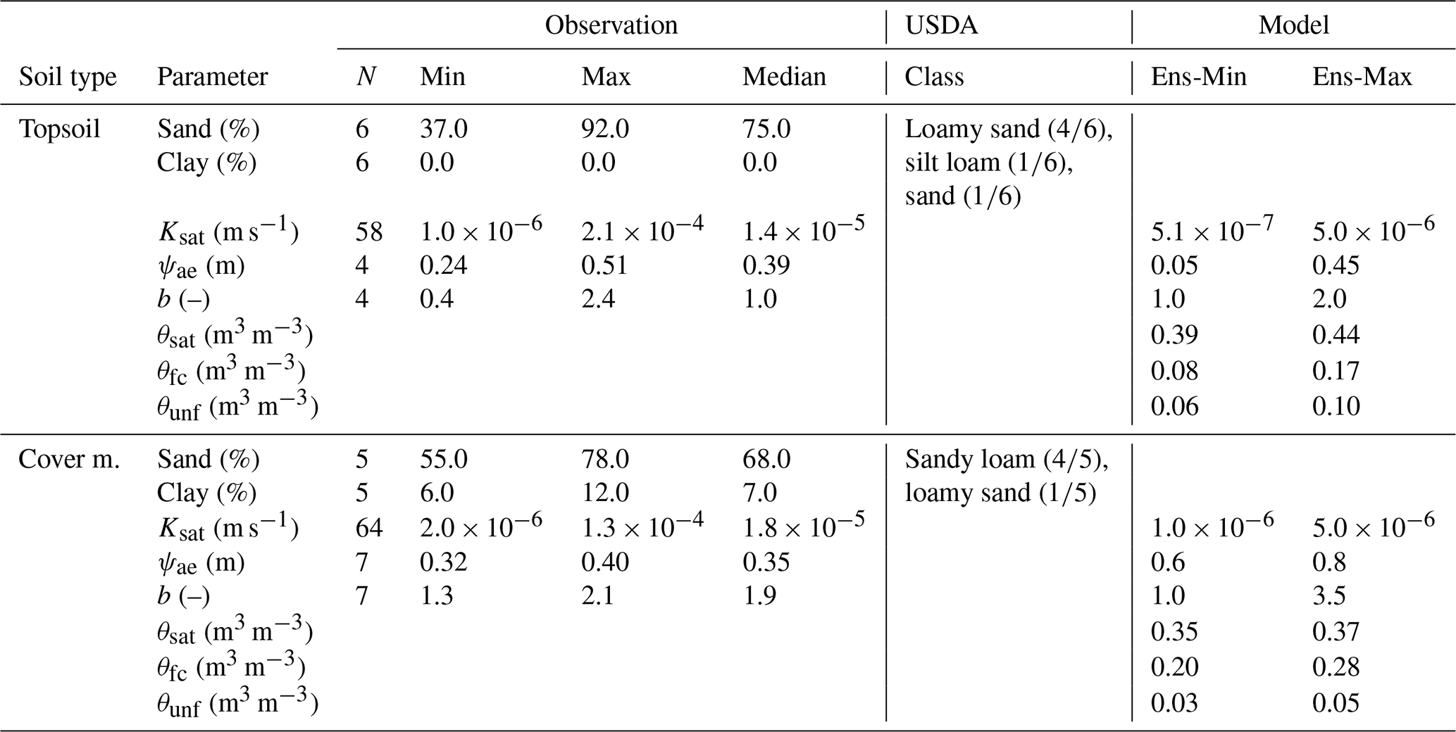
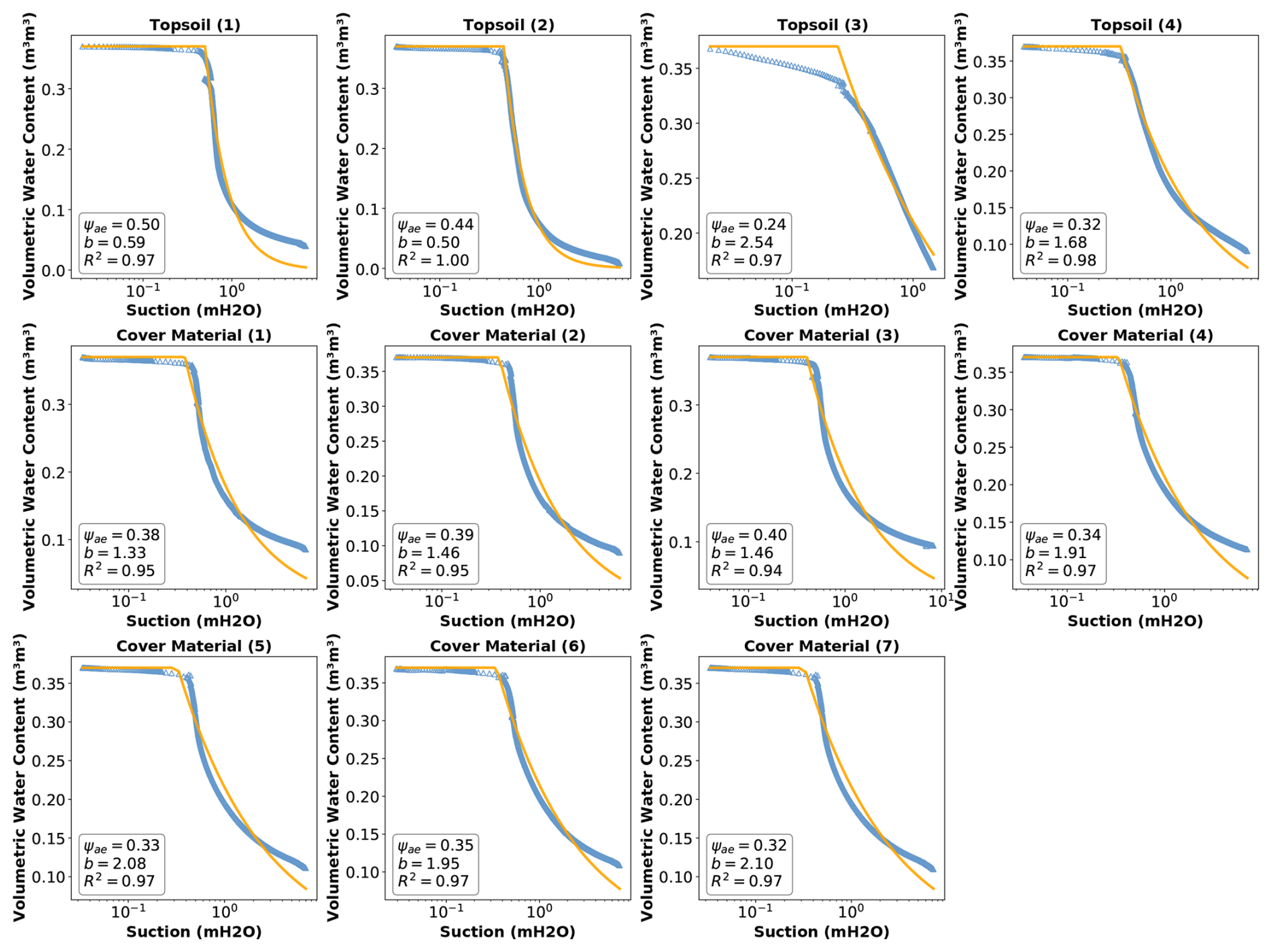
Figure 3 Soil water retention curves for the topsoil and cover materials used in the experimental plot. The blue triangles represent the measured data, and the solid lines are the fitted curves obtained using the soil water retention model of Clapp and Hornberger (1978). Each graph is annotated with the parameters of the Clapp and Hornberger soil water retention model, namely ψ_ae; b; and the coefficient of determination (R²), indicating the goodness of fit.

2.2 Data

The study site receives over 1050 mm of precipitation annually, with an average snowfall of 227 cm. Historically (1982–2017), the location experienced 109 d annually, with more than 3 cm of snow on the ground. While we had two on-site weather stations, their data were unsuitable due to large gaps and a significant underestimation of precipitation. Therefore, the meteorological forcing for SVS was mainly obtained from the Saint-Germain-de-Grantham (Saint-G in Fig. 2d) weather station, located 13 km from the site. No elevation correction was applied since the station is roughly at the same elevation (85 m for Saint-G. and 110 m for our study site). Shortwave and longwave radiation fields, unavailable at the weather station, were sourced from the ERA5 reanalysis (Hersbach et al., 2020). We estimated specific humidity from the dew-point temperature and atmospheric pressure using the MetPy meteorological Python library (May et al., 2022). The Saint-Germain-de-Grantham station uses a double Alter shield precipitation gauge. Precipitation measurements were adjusted for wind bias using the formula suggested by Kochendorfer et al. (2017). Rainfall and snowfall were distinguished using the equation proposed by Jennings et al. (2018) based on relative humidity and air temperature (Eq. 1):

$$\begin{array}{}\text{(1)}& P_{\mathrm{snow}}={\displaystyle \frac{\mathrm{1}}{\left[\mathrm{1}+\exp c_{\mathrm{1}}+\left(c_{\mathrm{2}}{T}_{\mathrm{a}}\right)+\left(c_{\mathrm{3}}\text{RH}\right)\right]}},\end{array}$$

where T_a is air temperature (°C); RH is the relative humidity (%); and c₁,c₂, and c₃ are empirical coefficients equal to −10.04, 1.41, and 0.09, respectively. Precipitation is recognized as snow if P_snow is greater than 0.5, and it is recognized as rain otherwise.

3 Methodology and model description

3.1 SVS land surface model

This study used the SVS land surface model, developed and maintained by ECCC (Alavi et al., 2016; Husain et al., 2016; Leonardini et al., 2021). SVS requires seven hourly meteorological inputs: air temperature, shortwave and longwave radiation, wind speed, specific humidity, atmospheric pressure, and precipitation. For snow-free conditions, initial values for soil moisture and soil temperature within each model's soil layer must be provided (throughout this article, soil moisture refers to the soil volumetric liquid-water content). Information about vegetation temperature and intercepted liquid-water content is also required. SVS divides each grid cell into four tiling components: (1) bare ground, (2) low or high vegetation, (3) snow over bare ground and low vegetation, and (4) snow under high vegetation. It uses a force–restore approach (Bhumralkar, 1975; Blackadar, 1976) for energy budget calculations and uses a one-layer representation of snow and the vegetation canopy. A detailed overview of the SVS snow accumulation and melt routine can be found in Leonardini et al. (2021). The Richards equation governs vertical water movement in the soil, solved using a finite-difference scheme (Verseghy, 1991). SVS uses Clapp and Hornberger's equations (Clapp and Hornberger, 1978) to model soil water retention (SWR) and vertical hydraulic conductivity (k_v):

$$\begin{array}{}\text{(2)}& \mathit{\theta }={\mathit{\theta }}_{\mathrm{sat}}{\left({\displaystyle \frac{\mathit{\psi }}{{\mathit{\psi }}_{\mathrm{ae}}}}\right)}^{-b^{-\mathrm{1}}},\end{array}$$

and

$$\begin{array}{}\text{(3)}& k_{\mathrm{v}}=k_{\mathrm{v},\mathrm{sat}}{\left[{\displaystyle \frac{\mathit{\theta }}{{\mathit{\theta }}_{\mathrm{sat}}}}\right]}^{\mathrm{2}b+\mathrm{3}},\end{array}$$

where ψ is soil matric potential (m), θ_sat is soil moisture at saturation (m³ m⁻³), and k_v,sat is the saturated vertical hydraulic conductivity of the soil (m s⁻¹). In Eqs. (2) and (3), b (unitless) and ψ_ae (m) are empirical parameters related to the slope of the water retention curve and the air entry value soil water potential (suction), respectively. SVS, by default, calculates percolation at the bottom of the soil column only when the soil moisture exceeds field capacity. Surface runoff is simulated when the precipitation rate exceeds the first layer's k_v,sat or when the soil pores are saturated with water. Notably, the current operational SVS version does not simulate soil freezing and thawing and its impact on infiltration (Alavi et al., 2016). We implemented a simple soil-freezing scheme based on the heat conduction algorithm of Hayashi et al. (2007) to address this limitation. Appendix A describes this scheme in detail.

3.2 Experiment design

The experimental plot was constructed in 2018. Due to the potential impact of plot stabilization, we excluded the first year of field data (deep percolation, soil temperature, and moisture) from the model's performance evaluation. Meteorological data from July 2018 to September 2019 are used for model spin-up, with simulations considered for evaluation running from September 2019 to October 2022. To ensure a more accurate representation of processes at the near-surface and the base, the 190 cm soil column had a varying vertical discretization. The top and bottom 15 cm segments were divided into 2.5 cm layers, while the middle section used 5 cm layers (totaling 44 layers). The lower hydraulic boundary was set as a seepage face to simulate the capillary barrier effect at the cover material–drainage layer interface (Scanlon et al., 2002, 2005). Median sand and clay content values (Table 1) are assigned to each layer. The experimental plot was fully covered with short grass, classified as low vegetation in SVS. Parameters for low vegetation, such as leaf area index (LAI), roughness length, heat capacity, albedo, stomatal resistance, and root depth, are derived from lookup tables containing values for 21 vegetation classes. An ensemble simulation strategy was used to address uncertainties in model parameter values and meteorological data. A total of 30 different scenarios were constructed for each, resulting in a 900-member ensemble. Simulations were done using a developed Python wrapper (https://github.com/Alireza-Amani/svspyed, last access: 20 March 2025) and the ECCC's high-performance computing (HPC) cluster.

3.3 Constructing the ensemble

3.3.1 Model parameters

We selected sampling intervals for six model parameters that influence the movement and storage of water in the soil column: saturated vertical hydraulic conductivity (k_sat), volumetric liquid-water content at saturation (θ_sat) and at field capacity (θ_fc), unfrozen residual water content (θ_unf; see Sect. A), ψ_ae, and the b coefficient (Eq. 2). We used a combination of laboratory measurements, field observations, and inverse modeling to determine the sampling range for these parameters. Soil moisture observations during the winter of 2019 helped to establish the θ_unf range. The initial sampling ranges for k_sat, ψ_ae, and b were informed by the laboratory measurements (Table 1), and that for θ_sat was informed by soil moisture measurements. For each perturbation scenario, we used suction threshold values ranging from 1.0 to 3.4 m (10 to 33 kPa) to determine θ_fc. For example, a specific combination of ψ_ae and b, along with a randomly chosen suction value from this range, would be used in Eq. (2) to calculate θ_fc for that scenario. Following the definition of initial sampling intervals for the parameters (k_sat, θ_sat, θ_fc, ψ_ae, and b), we further refined the sampling ranges using inverse modeling. This process involved a five-dimensional grid search (a total of 10 000 different combinations) using soil moisture data from April to September 2019. For each combination, we calculated errors between hourly simulated and observed soil moisture from sensors in both soil types. The combinations with the lowest errors for each soil type helped refine the final sampling ranges. We chose this period because it followed the first winter during which freeze–thaw cycles were likely to have impacted soil hydraulic properties. The final parameter ranges are indicated in Table 1 (under the “Ens-Min” and “Ens-Max” columns). Finally, Latin hypercube sampling (Loh, 1996) was used to create ensemble members, ensuring a well-distributed sample across the parameter space.

3.3.2 Meteorological forcing

We constructed the 30 meteorological scenarios by randomly perturbing the input variables according to the approach suggested by Charrois et al. (2016). This approach ensures physically consistent temporal variations in the perturbed data. We used a first-order autoregressive (AR1) model to calculate the perturbations:

$$\begin{array}{}\text{(4)}& P_t=\mathit{\varphi }{P}_{t-\mathrm{1}}+{\mathit{ϵ}}_t.\end{array}$$

In Eq. (4), P_t is the perturbation value at time t, ϕ is the parameter for the autoregressive model, and ϵ is a white-noise process with zero mean and σ² variance. ϕ is obtained by fitting the AR1 model to the time series of each variable, and the variance (σ²) is computed using the standard deviation of the residuals between the variables from the Saint-Germain-de-Grantham station and the corresponding variables from the on-site measurements (average of two stations) following Eq. (5).

$$\begin{array}{}\text{(5)}& {\mathit{\sigma }}^{\mathrm{2}}={\mathit{\sigma }}_{\mathrm{res}}(\mathrm{1}-{\mathit{\varphi }}^{\mathrm{2}})\end{array}$$

Different perturbations were applied depending on the variable: additive perturbations for air temperature, dew-point temperature, wind speed, and atmospheric pressure and multiplicative perturbations for shortwave radiation and relative humidity (limited to [0.8, 1.2] to avoid extremes), following Charrois et al. (2016). Longwave radiation values are perturbed within ±25 (W m⁻²) based on Raleigh et al. (2015). Rainfall is perturbed within ±5 % in accordance with the World Meteorological Organization's recommended range of uncertainty for automatic tipping-counter rain gauges (Lanza et al., 2005; Colli et al., 2013). Finally, the precipitation phase was determined after the perturbations were applied to air temperature and relative humidity.

3.4 Performance assessment

The performance of the SVS ensemble in simulating soil moisture, soil temperature, snow depth, and deep percolation was evaluated using the continuous ranked probability score (CRPS, Grimit et al., 2006; Matheson and Winkler, 1976). Following the formulation proposed by Stein and Stoop (2022), we evaluated the distance between the simulated and observed cumulative distribution functions (CDFs), denoted as F and G, respectively, based on the works of Baringhaus and Franz (2004) and Székely and Rizzo (2005):

$$\begin{array}{}\text{(6)}& \begin{array}{rl}\underset{-\mathrm{\infty }}{\overset{+\mathrm{\infty }}{\int }}\left[F\right(x)-G(x){]}^{\mathrm{2}}\text{d}x& ={\mathbb{E}}_{X,Y}\left(\right|X-Y\left|\right)\\ & -{\displaystyle \frac{\mathrm{1}}{\mathrm{2}}}\left[{\mathbb{E}}_{X,X^{\prime }}\right(|X-X^{\prime }|)\\ & +{\mathbb{E}}_{Y,Y^{\prime }}\left(\right|Y-Y^{\prime }\left|\right)],\end{array}\end{array}$$

where X and X^′ (Y and Y^′) represent independent copies of a random variable with a CDF given by F(G). For a given time step, we can calculate the CRPS of the SVS ensemble with the following (Stein and Stoop, 2022):

$$\begin{array}{}\text{(7)}& \begin{array}{rl}\text{CRPS}(F_x,G_y)& ={\displaystyle \frac{\mathrm{1}}{N}}{\displaystyle \frac{\mathrm{1}}{M}}\sum _{i=\mathrm{1}}^M\sum _{j=\mathrm{1}}^N|x_i-y_j|\\ & -{\displaystyle \frac{\mathrm{1}}{\mathrm{2}{M}^{\mathrm{2}}}}\sum _{j=\mathrm{1}}^M\sum _{k=\mathrm{1}}^M|x_j-x_k|\\ & -{\displaystyle \frac{\mathrm{1}}{\mathrm{2}{N}^{\mathrm{2}}}}\sum _{j=\mathrm{1}}^N\sum _{k=\mathrm{1}}^N|y_j-y_k|,\end{array}\end{array}$$

where x(j), with $j=\mathrm{1},\mathrm{\dots },N$, corresponds to the simulated values for an ensemble with N members, and y(i), with $i=\mathrm{1},\mathrm{\dots },M$, corresponds to the observed values for an observation ensemble of size M. The observation ensembles for soil moisture and soil temperature took into account both potential sensor errors and variability due to soil heterogeneity. Two sensors at each depth within the experimental plot made the latter possible. The manufacturer-reported sensor accuracies are ± 0.03 m³ m⁻³ and ±1 °C for soil moisture and soil temperature measurements, respectively. While acknowledging that applying manufacturer calibration functions to low-cost sensors like the 5TM may lead to larger deviations from the true soil moisture values (Mittelbach et al., 2012), our limited laboratory calibration exercise indicates that a ±0.03 m³ m⁻³ range is reasonable for these probes and the manufacturer's calibration equation in our soils. To construct the ensembles for soil moisture and soil temperature at each depth, we randomly perturbed the nominal values of each sensor a total of 30 times using a uniform distribution, resulting in an ensemble of size 60. Similarly, we applied random perturbations within the reported accuracy of ±1 cm for snow depth observations, creating a 60-member ensemble. Regarding the calculation of CRPS concerning deep percolation, where both lysimeters provided deep-percolation measurements, we used both values; if one lysimeter had missing data, only the available measurement was used. Additionally, to compare the ensemble mean of simulated and observed variables, we used Pearson's correlation coefficient and the mean bias error (MBE). The MBE was calculated by subtracting the observations from the simulated values. The evaluation metrics were calculated for cold (from November to March) and warm months, allowing us to assess seasonal variations in model performance.

4 Results

4.1 Snow depth

Figure 4 compares the measured and simulated daily snow depth from SVS and the weather station across three periods. The shaded area shows the 95 % confidence interval of the ensembles, with lines representing the ensemble mean. The vertically shaded areas highlight periods with potential rain-on-snow events. These periods (hours) are characterized by near- or above-zero (°C) air temperature and non-zero precipitation. The rain-on-snow events are important as they can significantly impact snowpack properties (Cohen et al., 2015; Juras et al., 2017; McCabe et al., 2007). Manual snow measurements taken on 10 different days at two locations (one near the enclosure, shown as squares, and one elsewhere on the site) are included in Fig. 4 for comparison. Each one of those 10 measurements is the average of 10 samples (snow water equivalent (SWE) and snow depth) along a path, taken with a Federal snow sampler. The close agreement between the weather station data and the manual measurements near the enclosure (MBE of −1.6 cm) suggests a reasonable agreement between the two measurements. Figure 4 also shows that the spread of observations is relatively low compared to the SVS ensemble. This narrow spread is because the uncertainty we have considered in the observations was limited to the sensor's expected accuracy range. It did not include spatial variability, which can be significant, as indicated by the manual snow measurements in the figure.

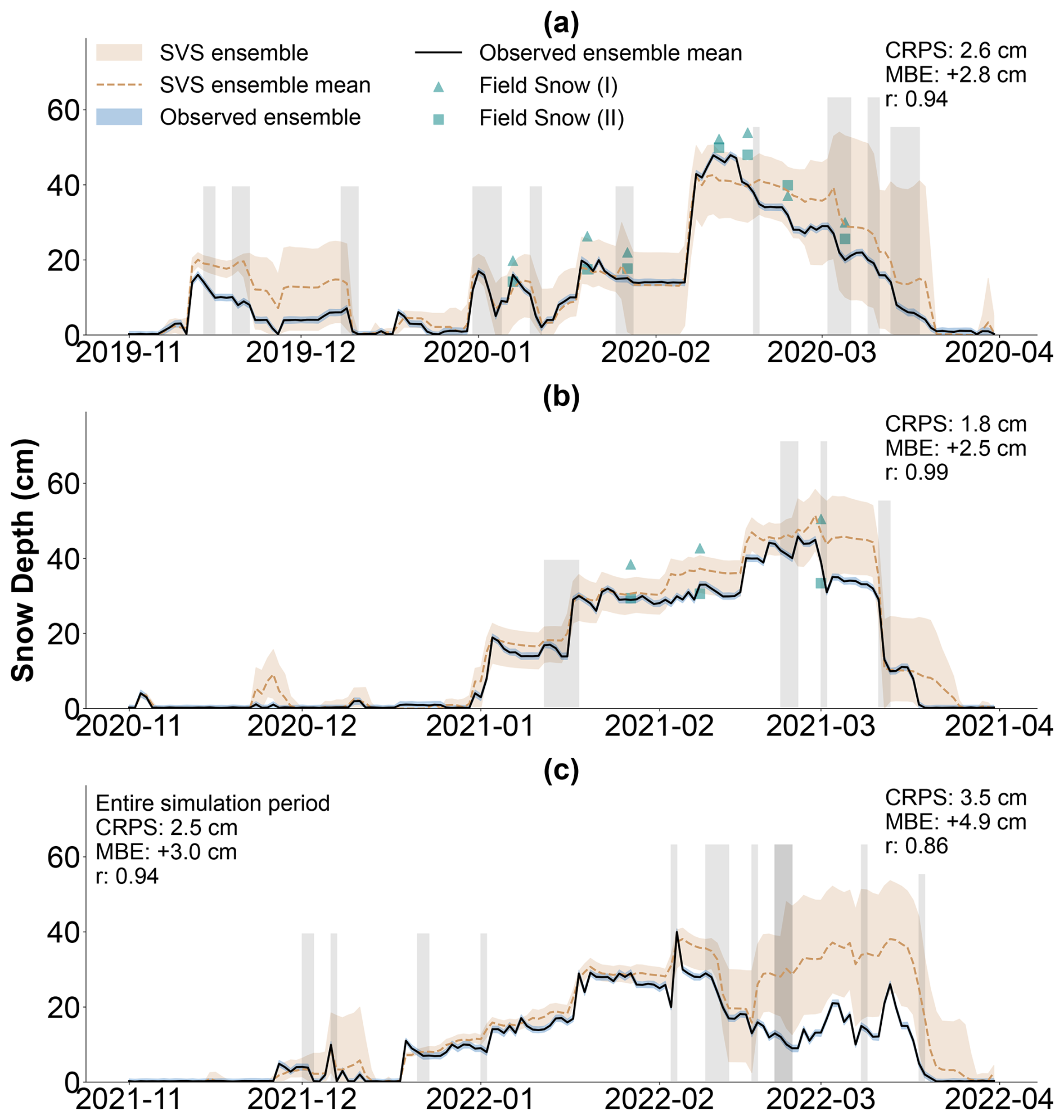
Figure 4 Daily snow depth (cm) for (a) November 2019 to April 2020, (b) November 2020 to April 2021, and (c) November 2021 to April 2022. The lines represent the ensemble mean of SVS and observations at the Saint-Germain-de-Grantham weather station, and the shaded area shows the 95  % confidence interval. The points represent manual snow measurements from two locations at the study site. The vertically shaded areas are indicators for periods with potential rain-on-snow events.

Figure 4 reveals a significant overlap between the SVS and snow depth observation ensemble. This agreement is reflected in a total CRPS of 2.5 cm for the combined periods. The correlation coefficient (r) between the ensemble means is high for November 2019 to April 2020 (0.94) and for November 2020 to April 2021 (0.99), indicating close agreement between the simulated and observed snowpack evolutions. However, the period between November 2021 and April 2022 shows a substantial overestimation of snow depth, starting on 17 February 2022. The snow depth for the SVS ensemble increases by 9 cm on average between 17 and 18 February, while this increase is only 3 cm based on observations. This divergence greatly impacted the evaluation metrics. Before 17 February, r is 0.98, with a slight positive bias (MBE +1.5 cm). The overestimation coincides with a potential rain-on-snow event (17 February), with temperature fluctuating above and below freezing and with substantial precipitation (24.9 mm). This suggests that the overestimation was likely to be due to a misclassification of the precipitation phase within the SVS ensemble. Figure 4c highlights the fact that this issue adversely affected model performance during late winter, a critical period with substantial snowmelt. The calculated CRPS and correlation coefficient for March 2022 (8.3 cm and 0.94) are noticeably worse than those for March 2020 (3.1 cm, 0.98) and March 2021 (3.8 cm, 0.98). Interestingly, the maximum snow depth consistently reaches a value close to 50 cm for the three winters, but no specific reason for this was identified in the data. However, it is important to note that, during the first two winters, the SVS ensemble mean closely matches the observed values at the times of peak snow depth.

4.2 Near-surface soil temperature and soil moisture

Figure 5 compares the simulated and observed daily soil temperatures at 75 mm depth, divided into three periods: (a) September 2019 to November 2020; (b) November 2020 to November 2021; and (c) November 2021 to November 2022, during which time no observations are available. The figure displays the ensemble means of the SVS model (gold-brown lines) and observations from lysimeters L1 (black lines) and L2 (purple lines), along with the 95 % confidence interval of the SVS ensemble (shaded area). The SVS model performs well in simulating near-surface soil temperature across the entire period, with a CRPS of 0.8 (°C) and a slight cold bias (−1.2 °C). The scatterplot in Fig. 7a further supports this, showing good performance during warm and cold months (from November to March). The low observed variability in soil temperature in Fig. 5 reflects both the low spatial variability within the enclosure and the sensors' accuracy. There are two notable gaps in the data: from March 2020 to May 2020 and from November 2020 and January 2021. These gaps are likely to have a small effect on the performance evaluation as they are mostly outside of the freezing period, and the model tends to simulate soil temperature well during this time.

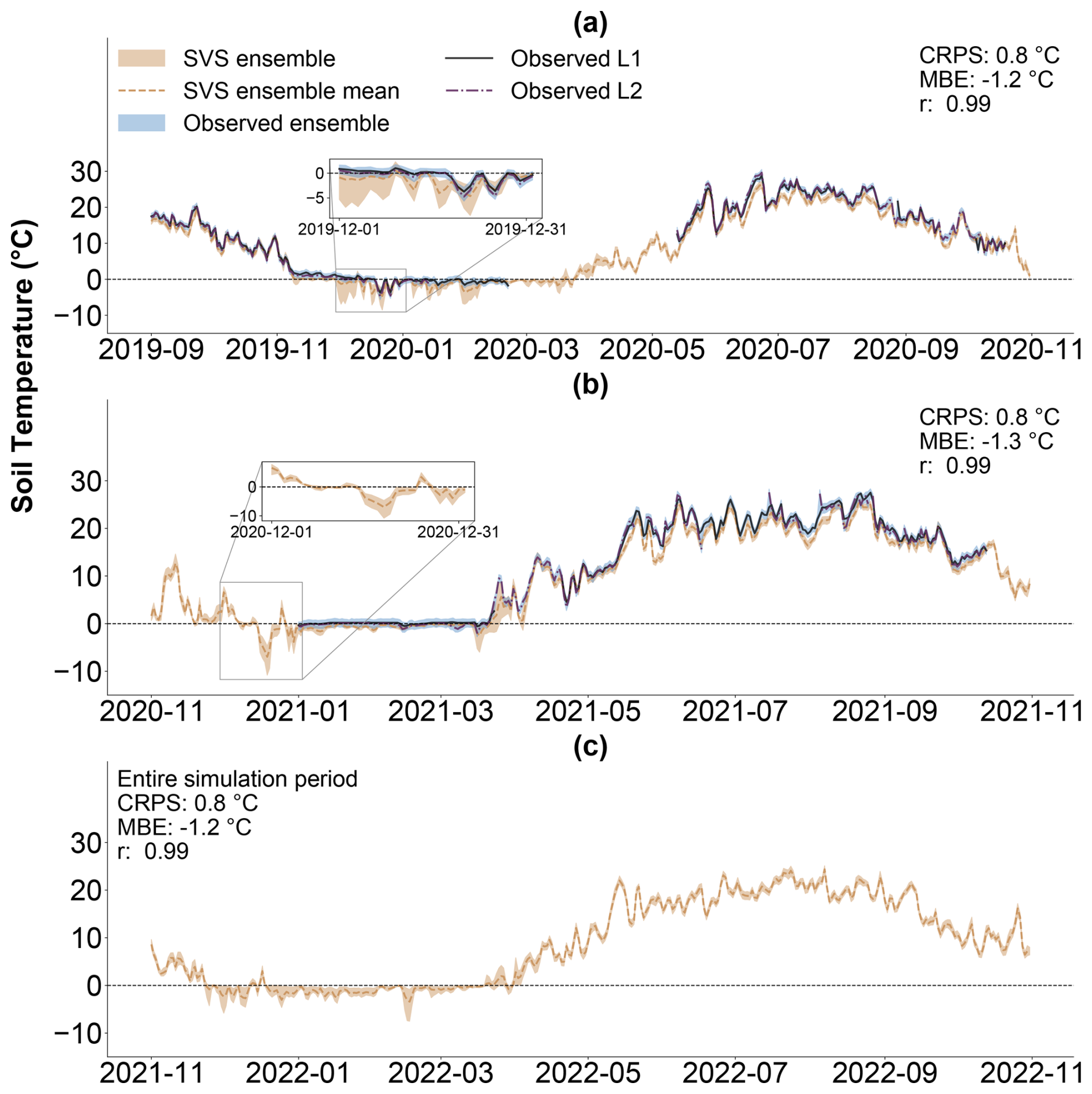
Figure 5 Daily averaged soil temperature at 75 mm depth (°C). (a) September 2019 to November 2020. (b) November 2020 to November 2021. (c) November 2021 to November 2022 (no observations available for this period). The lines represent the ensemble means of the SVS model (gold brown) and observations from lysimeters L1 (black) and L2 (purple). The shaded area represents the 95 % confidence interval of the ensembles. Insets in (a) and (b) show zoomed-in views of the data for specific periods.

Figure 6 compares the simulated and observed daily soil moisture at 75 mm depth. The model exhibits acceptable agreement with observations for most of the period, with a CRPS of 0.02 m³ m⁻³. However, we observe a consistent pattern of underestimation during February 2020, as well as during January and February 2021. This issue is illustrated in Fig. 7b, with a bias of −0.06 (m³ m⁻³) during cold months. During these periods, the SVS ensemble consistently assumed that the soil moisture was equal to the residual unfrozen water content due to the simulated soil freezing.

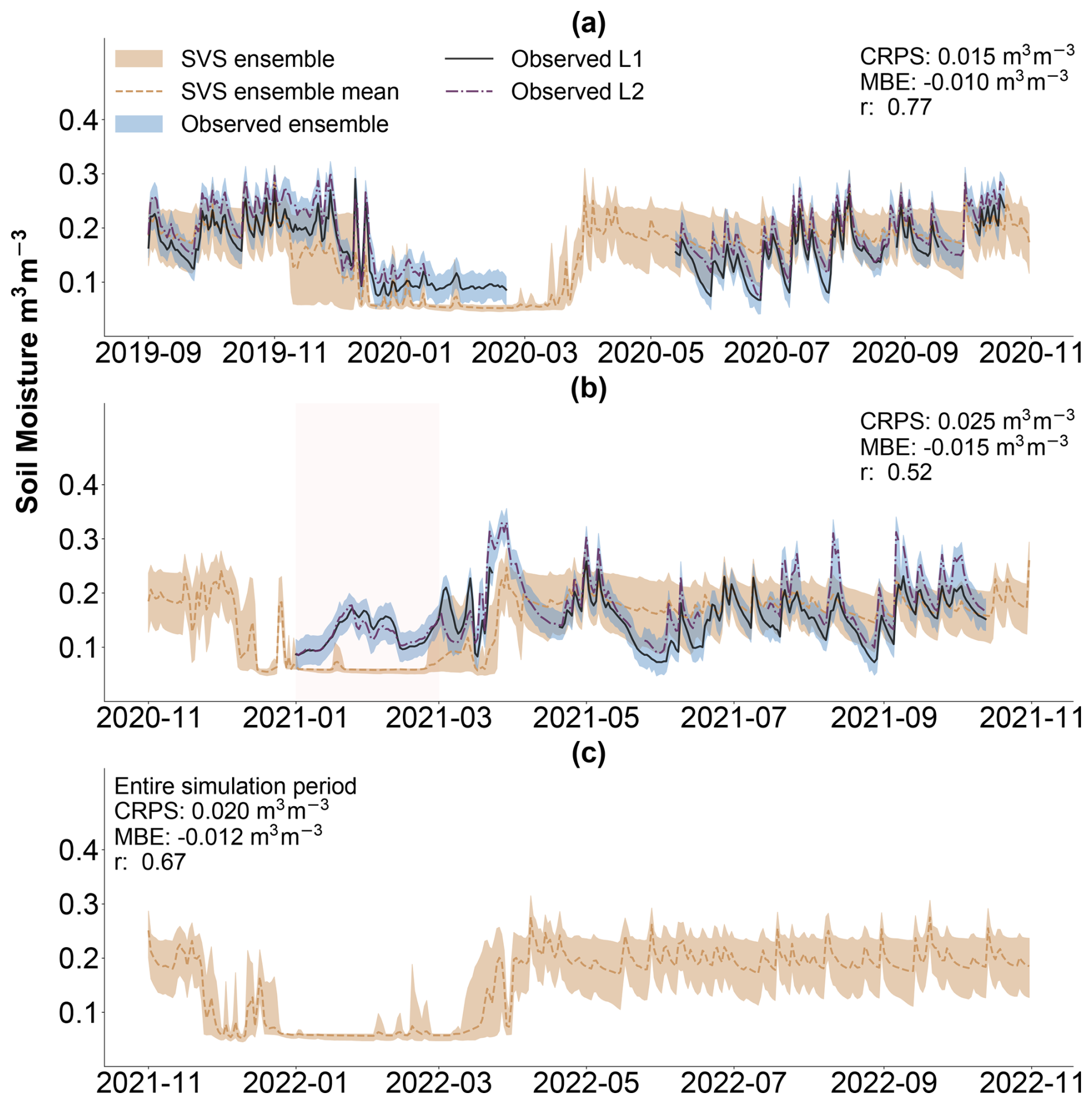
Figure 6 Daily averaged soil moisture at 75 mm depth (m³ m⁻³). (a) September 2019 to November 2020. (b) November 2020 to November 2021. (c) November 2021 to November 2022 (no observations available for this period). The lines represent the ensemble means of the SVS model (gold brown) and observations from lysimeters L1 (black) and L2 (purple). The shaded area represents the 95 % confidence interval of the ensembles.

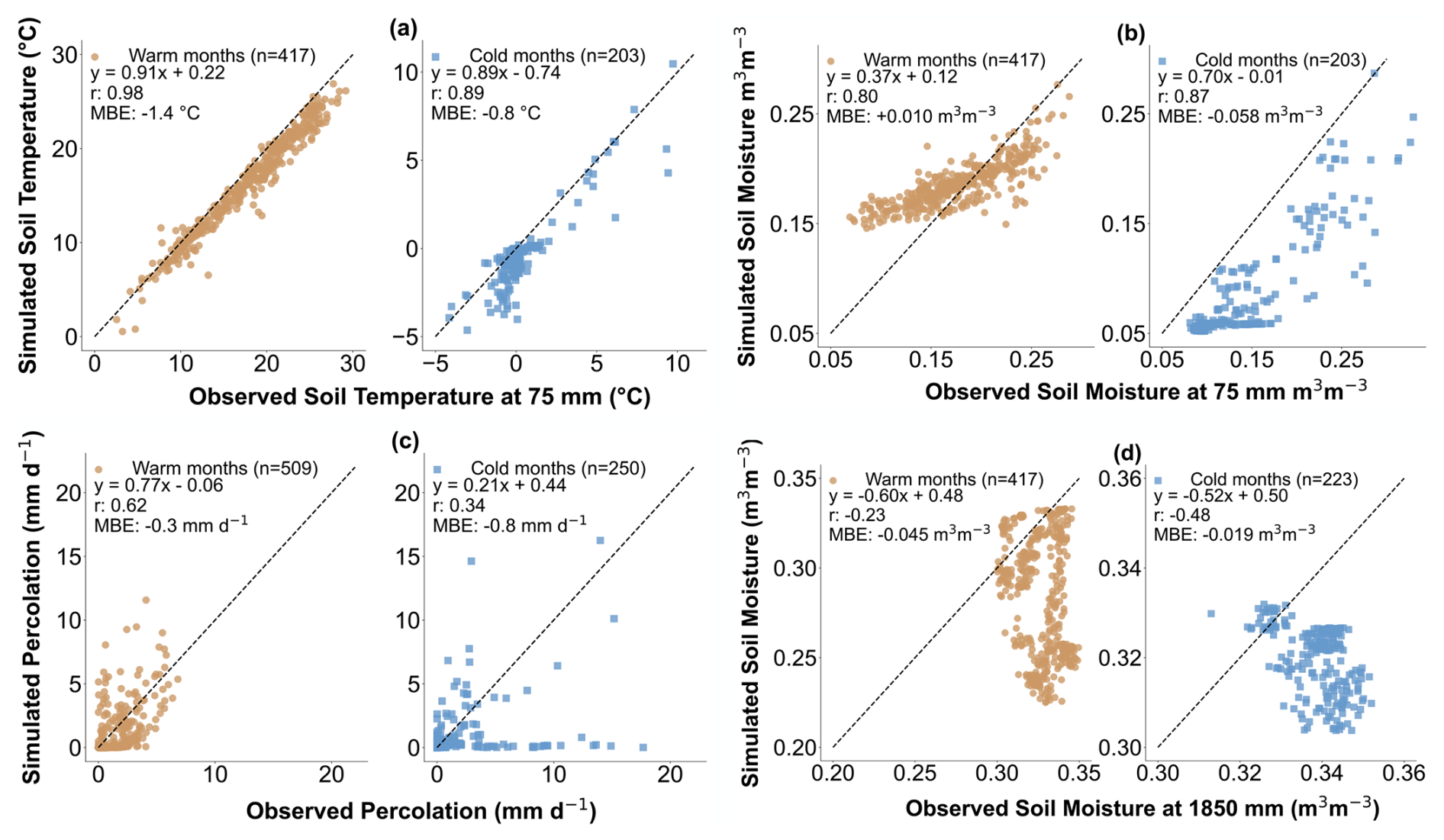
Figure 7 Scatterplots comparing daily simulated and observed ensemble means over the entire simulation period for different soil variables and seasons. (a) Soil temperature at 75 mm depth. (b) Soil moisture at 75 mm depth. (c) Deep-percolation rates. (d) Soil moisture at 1850 mm depth. Warm months (orange markers) are defined as April to October, while cold months (blue markers) are defined as November to March. Linear regression equations and model performance metrics (MBE and r) are shown for each plot, with the number of data points (n) indicated in parentheses.

4.3 Deep subsurface soil moisture

Figure 8 compares the simulated and observed daily soil moisture at 1850 mm depth, with Fig. 7d breaking down model performance by warm and cold months. From September 2019 to November 2020, the SVS ensemble closely matches the observations. This is reflected in the CRPS of 0.01 (m³ m⁻³). The model slightly underestimated (MBE: −0.02 m³ m⁻³) soil moisture during this period, most notably during the summer of 2020. SVS maintained a good performance until the summer of 2021, with Fig. 8b showing a substantial divergence between the simulated and observed ensembles. This is reflected in the considerably worse CRPS (0.04 m³ m⁻³) and MBE (−0.05 m³ m⁻³) values for November 2020 to November 2021. Figure 7d further emphasizes this underestimation bias during warm months. During cold months, however, as shown in Fig. 7d, there is a better performance by SVS, with an MBE equal to −0.019 m³ m⁻³. Importantly, the negative correlation coefficients associated with cold and warm months may suggest a mismatch between the modeled and actual lower boundary conditions within the soil profile. It is worth noting that the deep soil moisture data contain gaps from March 2020 to May 2020 and from November 2020 to January 2021, but these gaps are likely to have a minor impact on the overall analysis because, except for the summer months, the model and observations align closely in terms of absolute values.

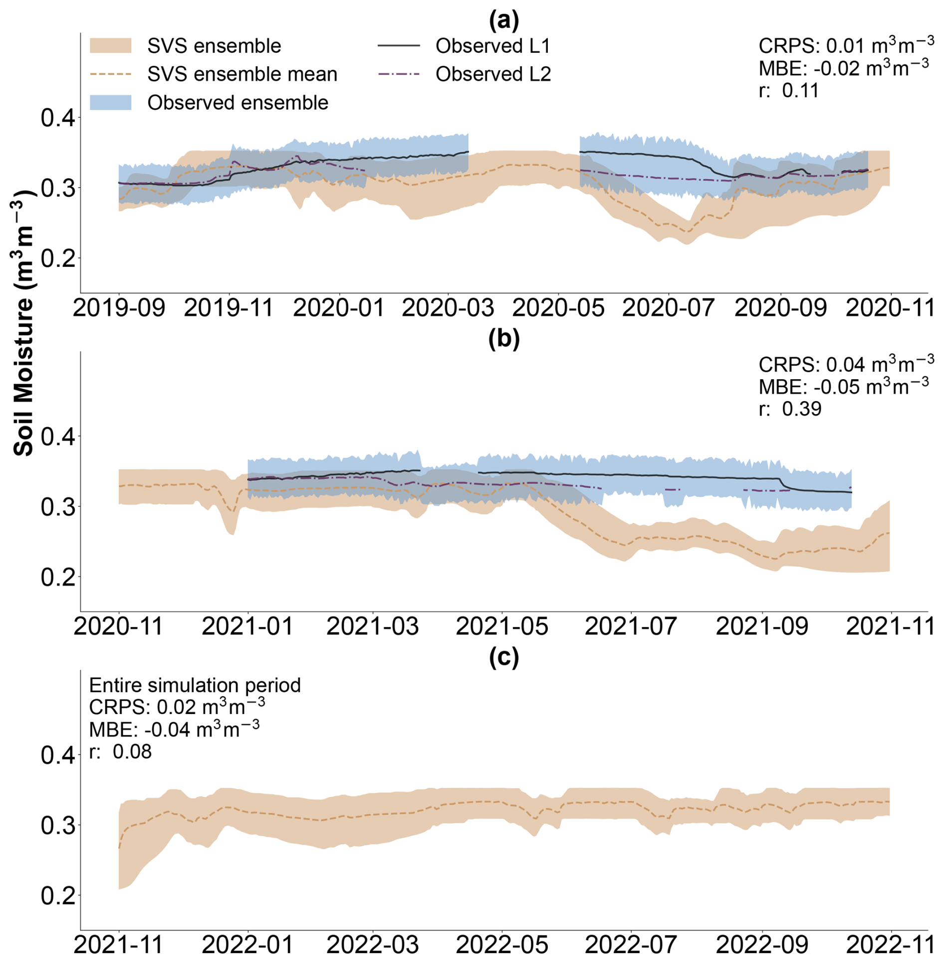
Figure 8 Daily averaged soil moisture at 1850 mm depth (m³ m⁻³). (a) September 2019 to November 2020. (b) November 2020 to November 2021. (c) November 2021 to November 2022 (no observations available for this period). The lines represent the ensemble means of the SVS model (gold brown) and observations from lysimeters L1 (black) and L2 (purple). The shaded area represents the 95 % confidence interval of the ensembles.

4.4 Deep percolation

Figure 9 compares the simulated and observed daily deep-percolation rates from September 2019 to November 2022, with Fig. 7c further examining warm- and cold-month performances. The CRPS values may indicate a good agreement between SVS and observations: 0.6 mm d⁻¹ from September 2019 to November 2020, 0.2 mm d⁻¹ from November 2020 to November 2021, and 0.8 mm d⁻¹ from November 2021 to November 2022. However, Fig. 9 shows that SVS struggles to match the temporal dynamics of deep percolation closely; this is most notable in October 2019, March 2020, and winter 2022. Despite this limitation, Fig. 9a shows that the SVS ensemble mean follows observations of major percolation events reasonably well, including those driven by snowmelt (e.g., April 2020) and significant rainfall (e.g., 83.4 mm on 3 and 4 August and 50.3 mm on 29 August 2020). While there is a minor negative bias until November 2021 (MBE: −0.2 mm d⁻¹), this underestimation increases significantly after November 2021 (MBE: −1.5 mm d⁻¹). This change is largely attributable to SVS missing several large deep-percolation events during winter 2022, as is also evident in Fig. 7c. Investigating the results reveals that, from 1 January 2022 to 31 March 2022, there were 23 d in which the L1 lysimeter collected more than 1 mm of deep percolation (in total, 176.8 mm), whereas the ensemble mean values were smaller than 1 mm (in total, 2.8 mm). This limitation explains the notably better performance during warm months (r: 0.62, MBE: −0.3 mm d⁻¹) compared to during colder months (r: 0.34, MBE: −0.8 mm d⁻¹).

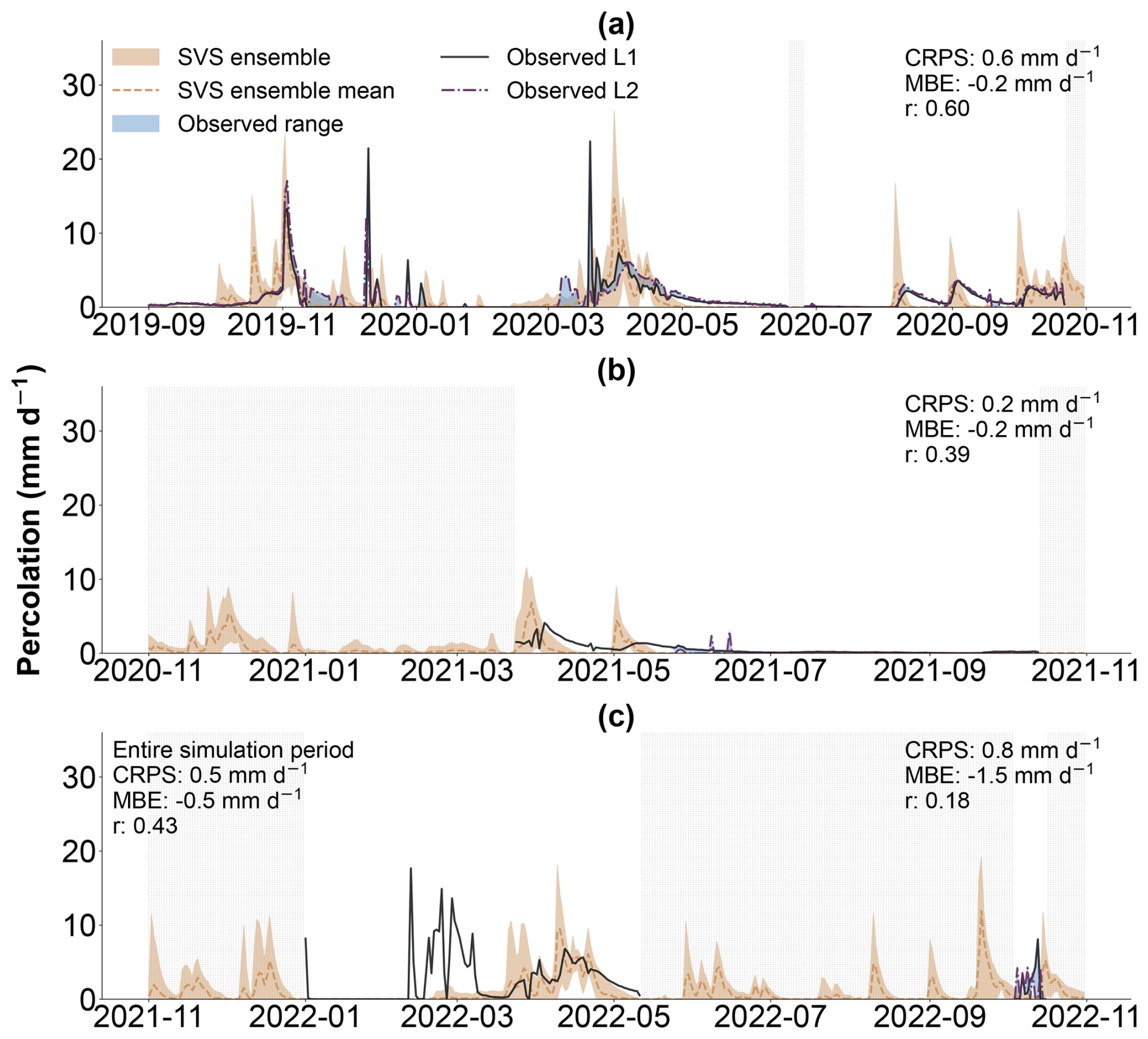
Figure 9 Daily deep-percolation rates (mm d⁻¹). (a) September 2019 to November 2020. (b) November 2020 to November 2021. (c) November 2021 to November 2022. The lines represent the ensemble means of the SVS model (gold brown) and observations from lysimeters L1 (black) and L2 (purple). The shaded area represents the 95 % confidence interval of the SVS ensemble. Gray-shaded areas indicate periods where observations from both lysimeters were unavailable.

5 Discussions

The results highlight the potential of SVS to simulate key hydrological processes influencing deep percolation. Yet, they also revealed important discrepancies with field data. These discrepancies raise questions such as the following: (i) why is there a slight cold bias in near-surface soil temperature? (ii) What are the underlying reasons for the limitations in the model's ability to represent the dynamics of near-surface soil moisture during winter? (iii) What limits the model's ability to simulate subsurface soil moisture? (iv) How do these limitations influence deep percolation? In this section, we further investigate these questions.

5.1 Cold bias in SVS during snow-free conditions

A potential limitation within SVS is its underestimation of near-surface soil temperature during snow-free conditions with below-freezing air temperatures. This cold bias is evident in December 2019 and 2020 in Fig. 5. This is likely to be due to the model's simplified handling of soil temperature dynamics under such conditions. Currently, the soil-freezing scheme in the SVS model uses the surface temperature from a force–restore (FR) approach as its upper boundary condition. The FR approach in SVS neglects the latent heat release that occurs during soil freezing and thawing (Husain et al., 2016), which can significantly impact soil temperature profiles. As shown by Boone et al. (2000), incorporating these latent heat effects into force–restore schemes improves soil temperature simulations during freezing periods. Therefore, neglecting this aspect in SVS likely contributes to underestimating surface soil temperature in early-winter snow-free conditions. This, in turn, affects the ground heat flux calculations used by the soil-freezing scheme, potentially leading to an overestimation of frost depth. To better understand the potential for frost depth overestimation, future studies can gain a more comprehensive understanding by analyzing soil temperature at deeper soil depths. Although there are 600 mm depth soil temperature sensors in the E1 enclosure, their data were unavailable for December 2019 and 2020, preventing direct assessment of the frost depth during this period.

5.2 Limitations of SVS in simulating soil moisture and deep percolation in winter

While potential limitations in SVS's soil-freezing scheme exist, these may not fully explain the discrepancy in terms of near-surface soil moisture during winter 2021 (Fig. 6b). Despite accurate soil temperature simulations (CRPS of 0.3 °C), soil moisture simulation significantly deviated in this period (CRPS of 0.05 m³ m⁻³). This highlights potential shortcomings in representing hydrological processes under freezing conditions. Currently, SVS lacks the representation of water infiltration due to macropores in frozen soil, a complex process that can largely impact soil moisture dynamics (Watanabe et al., 2013; Jiang et al., 2021; Stähli et al., 1996; Mohammed et al., 2018). This limitation is likely to be the main factor explaining the aforementioned discrepancy. It could also explain the missed deep-percolation events during the winter of 2022 (Fig. 9). In freezing conditions, snowmelt or rainfall can infiltrate and bypass frozen near-surface soil through preferential flow paths (macropores), directly reaching deeper soil layers (Demand et al., 2019; Watanabe and Kugisaki, 2017). Without accounting for this process, the model might underestimate deep percolation while overestimating surface runoff during freezing periods.

To further illustrate the model's limitations and their potential impacts, we examined a specific event in December 2019 (from the 9th through the 12th) where SVS did not simulate deep percolation. Figure 10 presents the relevant data. Figure 10a shows a likely rain-on-snow event with potentially considerable snowmelt infiltration during a warmer period. Figure 10b reveals that the near-surface soil was likely to be frozen during the snowmelt event. It also indicates a good agreement between the simulated (ensemble mean) and observed (on top of the L2 lysimeter) soil temperatures (MBE: −0.8 °C). Interestingly, Fig. 10c and d show that the infiltrated water bypassed the surface soil, directly reached the lysimeter (L2) base, and generated a significant deep-percolation volume (18.2 mm). This hints at water movement through preferential flow paths. In contrast, the SVS model (ensemble mean) simulated no significant percolation and instead generated a considerable amount of surface runoff (29.2 mm). These findings are consistent with the results of Mohammed et al. (2019), who studied the impacts of preferential flow on snowmelt partitioning and groundwater recharge in frozen soils at three grassland sites in the Canadian Prairies. They found that preferential flow paths, likely created by macropores in the soil, allowed for rapid infiltration and bypass flow, even when the ground was frozen, significantly influencing the partitioning of snowmelt into infiltration or runoff and, therefore, the amount of water available for groundwater recharge. It is also important to acknowledge that the lysimeter itself, by its design, could influence the occurrence and patterns of preferential flow events, potentially amplifying or altering natural flow paths (Williams et al., 2019, 2020). Further investigation is needed to understand how these factors contribute to the discrepancies observed between the simulated and observed soil moisture and deep percolation, especially under freezing conditions.

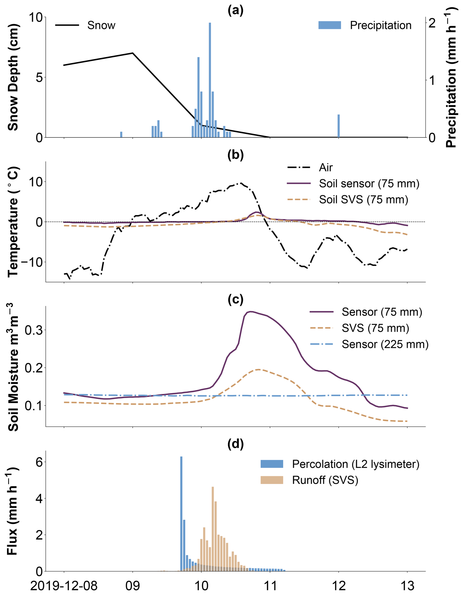
Figure 10 Time series (9 December 2019 to 13 December 2019) of (a) snow depth (cm) and precipitation (mm h⁻¹), (b) air and soil temperature at 75 mm below the surface (°C), (c) observed and simulated soil moisture at 75 and 225 mm below the surface (m³ m⁻³), and (d) percolation from the L2 lysimeter (mm h⁻¹) and simulated surface runoff (mm h⁻¹).

5.3 Influence of capillary barrier on simulated subsurface soil moisture

Figure 7d reveals a negative correlation coefficient between simulated and observed subsurface soil moisture (1850 mm) for both cold and warm months. This limitation in accurately simulating the dynamics of the soil moisture at the bottom of the soil column is potentially related to the choice of the lower hydraulic boundary condition in the model. We adopted a seepage face boundary condition as it is often suggested in studies involving lysimeters to approximate the capillary barrier effect induced by the inclusion of the drainage layer at the bottom of the lysimeters (Scanlon et al., 2002, 2005). The capillary barrier increases water storage in the finer layer situated just above, potentially keeping this finer layer close to saturation (Mancarella and Simeone, 2012; Abdolahzadeh et al., 2011). Our results suggest that a more sophisticated boundary condition is required to more accurately reproduce the temporal variation of soil moisture close to a capillary barrier (Gao et al., 2023; Hübner et al., 2017; Kahale and Cabral, 2024). Figure 8 reveals that the simulated ensemble has a relatively high overlap with the observations during the cold months, during which the movement of water in the soil is predominantly downward, reflected in a small CRPS value of 0.007 m³ m⁻³, which is likely influenced by the inherent stability of deep soil moisture during this period. However, a notable underestimation occurs during warm months, particularly during the summers of 2020 and 2021, with CRPS values equal to 0.036 (m³ m⁻³), significantly worse than 0.007.

To further analyze the summertime underestimation, Fig. 11 compares simulated (ensemble mean) and observed (sensors inside and outside the L1 lysimeter) soil moisture at different depths from May to September 2020. Figure 11c reveals that the underestimation becomes increasingly pronounced during the warmer months. Figure 11b shows a similar, though less severe, underestimation at 1750 mm. Interestingly, the simulated soil moisture at 1750 mm agreed better with the sensor located outside (“ext” in Fig. 11b) the lysimeter, where no capillary barrier effect was present. The sensor's data revealed a drying pattern similar to the model, hinting at the influence of the lysimeter on the upward movement of water (the drying front) from deeper soil layers (Oldecop et al., 2017). Analysis of the L2 lysimeter data reveals the same pattern of divergence between simulated and observed soil moisture. This finding resonates with the findings of McCartney and Zornberg (2010), who investigated the zone of influence of a (geosynthetic) capillary barrier at the bottom of a laboratory-constructed 1350 mm soil column. During a 3-month evaporation stage (using heat lamps), their soil moisture measurements did not show a significant decrease beyond 700 mm below the surface. In other words, the drying front only progressed 700 mm into the soil layer.

Figure 11a reveals a notable divergence between the simulated and observed near-surface soil moisture (at 75 mm depth), where the SVS model consistently overestimates soil moisture throughout the entire period from May to September 2020, and this overestimation becomes particularly pronounced during the summer months (July and August). This raises questions about potential contributing factors. Did the no-flux boundary walls of the lysimeter or the capillary barrier alone contribute to this discrepancy? Could the limitations of the one-dimensional single-continuum representation of the model in capturing the complex dynamics of water movement and storage in the vadose zone contribute to this discrepancy? While errors in evapotranspiration estimation could play a role, the absence of direct measurements limits our ability to fully quantify their impact. A thorough evaluation of the effects on deep-percolation simulations necessitates more integrated data, including deep-percolation and soil moisture measurements, particularly during summer.

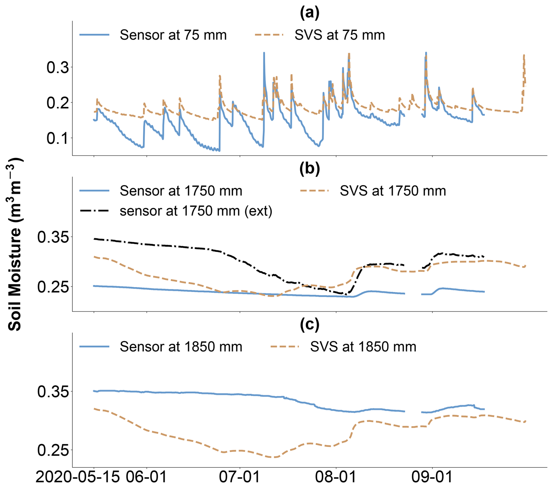
Figure 11 Time series (15 May–1 September 2020) of simulated (ensemble mean) and observed (the L1 lysimeter) daily soil moisture (m³ m⁻³) at different depths: (a) 75 mm, (b) 1750 mm, and (c) 1850 mm. Note that “ext” indicates a soil moisture sensor outside the L1 lysimeter.

This study's parameter estimation, based on inverse modeling (Sect. 3.3.1), used data from April to September 2019. While lysimeters offer controlled conditions for hydrological studies, they can change over time, influencing hydrological processes. Séré et al. (2012) highlight how changing soil properties within lysimeters can affect water flow and solute transport. The discrepancy between the model and observations, including the discrepancy shown in Fig. 11a, could be partly attributed to such temporal changes. Future studies with longer datasets can monitor lysimeter soil properties and use multi-year calibration to assess the impact of these changes on hydrological simulations.

6 Conclusions

Robust process-based evaluation of land surface models is critical for improving their ability to simulate deep percolation, particularly in cold regions where complex hydrological processes interact. Previous model evaluation studies often neglected the potential influence of uncertainties in forcing data, parameter values, and observations. Evaluations frequently relied on data with a coarse temporal resolution and rarely included processes such as snow and soil freezing. This study addresses these critical gaps. We comprehensively evaluate the Soil, Vegetation, and Snow (SVS) land surface model using high-resolution data from a large instrumented experimental plot built at the St-Nicéphore landfill site in southeastern Quebec, Canada. Our performance assessment approach accounted for uncertainty in meteorological inputs, a subset of the model's hydraulic parameters, and observations. Furthermore, we evaluated a newly implemented soil-freezing scheme within the SVS model for the first time.

The results showed that the simulated and observed daily snow depth correlated well for most of the simulation period, with a correlation coefficient (r) greater than 0.94 and a mean bias error (MBE) smaller than 3.0 cm. This suggests a good representation of snow accumulation and ablation processes within SVS. The soil-freezing scheme simulated near-surface daily soil temperature very well in cold months (r: 0.89), with a slight cold bias (MBE: −0.8 °C) due to potential shortcomings in representing the latent heat exchange during freezing and thawing cycles. SVS showed promise in capturing deep-percolation events driven by spring snowmelt and heavy summer and fall rainfall events. However, the model exhibited limitations in simulating deep percolation during cold months (r: 0.35) and under freezing conditions due to a lack of representation for infiltration in frozen soil and the influence of preferential flow pathways. These limitations also negatively impacted SVS's ability to simulate near-surface soil moisture during winter (MBE: −0.058 m³ m⁻³).

Our findings underscore challenges and important considerations for accurately simulating cold-region deep-percolation dynamics (Niu and Yang, 2006; Agnihotri et al., 2023). Future studies can focus on improving the representation of frozen-soil infiltration and preferential flow pathways within SVS and, potentially, in other land surface models. Furthermore, a detailed sensitivity analysis investigating the impact of individual parameters and meteorological forcing on model performance would be valuable for identifying the key factors driving model uncertainty and for guiding future model development and calibration efforts. However, until these limitations are addressed, SVS cannot be considered to be a fully reliable tool for simulating deep percolation in cold environments. Prioritizing the collection and subsequent open-access sharing of long-term, high-resolution integrated field measurements can facilitate such model improvements. Expanding model evaluations to include other cold regions, longer periods, and diverse land covers is essential for developing robust cold-region hydrological models. This approach, along with considering other limitations of the LSMs (Vereecken et al., 2019), can further improve deep-percolation simulation by land surface models and enhance our understanding of cold-region hydrology and its response to a changing climate.

Appendix A: Soil-freezing module in SVS

SVS uses a hybrid approach that combines force–restore schemes to compute the surface energy budget of bare ground, vegetation, and snow (Husain et al., 2016) with a multi-layer hydrological module solving the Richards equations for unsaturated flow in porous media (Alavi et al., 2016). This hybrid approach initially prevented the simulation of soil freezing and thawing by the model. To overcome this limitation, a new module has been developed.

The representation of soil freezing in SVS relies on the soil-freezing and soil-thawing module available in the Versatile Soil Moisture Budget model (VSMB, Mohammed et al., 2013). This module is based on the simple heat conduction algorithm of Hayashi et al. (2007) and simulates the evolution of soil temperature and associated phase changes without the computationally expensive iterative solution of coupled non-linear equations. In SVS, soil temperature and phase changes are solved on the same vertical grid as the hydrological processes using upper boundary conditions provided by the force–restore schemes solving the multiple energy budgets at the surface (Husain et al., 2016).

A1 Heat conduction algorithm

In the soil temperature algorithm, the heat conduction between two adjacent soil layers (upper to lower) is given by the following:

$$\begin{array}{}\text{(A1)}& q_{\mathrm{h}}=-{\mathit{\lambda }}_{\mathrm{s}}{\displaystyle \frac{{\mathrm{\Delta }}_{z}T}{\mathrm{\Delta }z}},\end{array}$$

where q_h is the soil heat flux (W m⁻²), Δ_zT is the difference in soil temperature between adjacent layers (lower minus upper) (K), Δz is the distance between the centers of the layers (m), and λ_s is the bulk thermal conductivity given by the thickness-weighted harmonic mean conductivity of the two layers (W K⁻¹ m⁻¹).

For a given soil layer j, the net heat flux (Δ_zq_h,j) is then computed as follows:

$$\begin{array}{}\text{(A2)}& {\mathrm{\Delta }}_z{q}_{\mathrm{h},j}=q_{\mathrm{h},j-\mathrm{1}}-q_{\mathrm{h},j}.\end{array}$$

The soil temperature algorithm assumes then that the change in net heat flux corresponds to a change in heat stored as sensible and latent heat in layer j:

$$\begin{array}{}\text{(A3)}& {\mathrm{\Delta }}_z{q}_{\mathrm{h},j}=({\mathrm{\Delta }}_t{T}_j{c}_{\mathrm{s},j}+{\mathrm{\Delta }}_t{w}_{i,j}{\mathit{\rho }}_{\mathrm{w}}{L}_{\mathrm{f}})d_j,\end{array}$$

where Δ_tT_j (K) and Δ_tw_i,j (kg kg⁻¹) are the changes in the soil temperature and liquid-equivalent ice content of layer j, respectively, with time; ρ_w is the density of water (kg m⁻³); L_f is the latent heat of fusion (J kg⁻¹); d_j is the layer thickness (m); and c_s,j is the volumetric heat capacity of the soil layer (J m⁻³ K⁻¹).

The VSMB soil-freezing scheme assumes that water in soil pores freezes at T_ref=273.15 K and ignores the freezing-point depression (Kurylyk and Watanabe, 2013). It accounts for the presence of unfrozen water that remains in the soil at sub-zero temperatures and co-exists with ice. The default VSMB algorithm assumes that the residual unfrozen water content w_l,r is constant and equals 0.06 by default. This option has been used in this work since it corresponds well to local observations of residual liquid-water content in frozen conditions. Another option in SVS allows the unfrozen residual water content to depend on the soil texture based on Niu and Yang (2006). If a soil layer j is completely thawed or frozen, with no liquid water above the residual frozen-water content (i.e., T_j≠T_ref), Δ_zq_h,j is converted to sensible heat until T_j reaches T_ref, and any residual is converted to latent heat (melting or freezing). If the soil is already frozen (T_j=T_ref), Δ_zq_h,j is first used for the phase change of all available liquid water above w_l,r, and any residual is converted to sensible heat. Calculations are performed sequentially from the top to the lowest soil layer.

The thermal heat capacity c_s and thermal conductivity λ_s of the soil layers are parameterized following Peters-Lidard et al. (1998) as functions of soil moisture and texture (percentage of sand and clay) and account for the effect of soil freezing as described in Boone et al. (2000). The dry-soil thermal conductivity and soil thermal conductivity are taken from He et al. (2021) and Johansen (1975), respectively.

A2 Lower boundary condition

The heat flux at the bottom of the lowest soil layer is specified using an annual mean deep soil temperature T_btm and an appropriate scaling depth z_btm. This is written as follows:

$$\begin{array}{}\text{(A4)}& q_{\mathrm{h},N}={\mathit{\lambda }}_{\mathrm{s},N}{\displaystyle \frac{T_N-T_{\mathrm{btm}}}{(z_{\mathrm{btm}}-z_N)}},\end{array}$$

where N corresponds to the deepest soil layer. In this study, T_btm was set to 7.5 (°C), and z_btm was set to 5 m.

A3 Upper boundary condition

The upper boundary condition accounts for the surface tiling used in SVS. It includes contributions from (i) snow-free bare ground, (ii) snow-free low and high vegetation, (iii) snow over bare ground and low vegetation, and (iv) snow below high vegetation. The heat flux at the top of the superficial soil layer is written as follows:

$$\begin{array}{}\text{(A5)}& q_{\mathrm{h},\mathrm{0}}=f_{\mathrm{grnd}}{H}_{\mathrm{grnd}}+f_{\mathrm{veg}}{H}_{\mathrm{veg}}+f_{\mathrm{snw}}{H}_{\mathrm{snw}}+f_{\mathrm{snwv}}{H}_{\mathrm{snwv}},\end{array}$$

where f_grnd and f_veg are the fractions of snow-free bare ground and snow-free low and high vegetation, respectively. f_snw and f_snwv represent the fraction of low vegetation and bare ground covered by snow and the fraction of soil under high vegetation covered by snow, respectively. H_grnd, H_veg, H_snw, and H_snwv are the heat flux (W m⁻²) from snow-free bare ground, snow-free vegetation, snow over bare ground and low vegetation, and snow below high vegetation.

For bare ground, the heat flux depends on the difference between the skin-temperature T_gs simulated by the force–restore approach for bare ground and the temperature of the upper soil layer (j=1). This is written as follows:

$$\begin{array}{}\text{(A6)}& H_{\mathrm{grnd}}={\displaystyle \frac{T_{\mathrm{gs}}-T_{\mathrm{1}}}{R_{\mathrm{g}}}}\text{ with }{R}_{\mathrm{g}}={\displaystyle \frac{d_{\mathrm{1}}}{\mathrm{2}{\mathit{\lambda }}_{\mathrm{s},\mathrm{1}}}}.\end{array}$$

In its current version, the soil-freezing scheme has no feedback on the force–restore scheme used for bare ground. Therefore, the prognostic temperature variables of the force–restore scheme used for bare ground lack the effect of latent heat release due to soil freezing and thawing. This can lead to an underestimation of soil temperature during soil freezing and an overestimation of soil temperature during soil thawing.

For snow-free low and high vegetation, SVS relies on the thermal coupling approach used in the EC-Land scheme (Boussetta et al., 2021). It uses the concept of skin conductivity to compute the heat exchanges between the vegetation tile and the soil. The heat flux between the snow-free low and high vegetation and the upper soil layer is written as follows:

$$\begin{array}{}\text{(A7)}& H_{\mathrm{veg}}=\left(T_{\mathrm{vs}}-T_{\mathrm{1}}\right),{\mathrm{\Lambda }}_{\mathrm{v}}\end{array}$$

where T_vs is the vegetation skin temperature simulated by the force–restore approach, and T₁ is the temperature of the upper soil layer. Λ_v is the skin conductivity (W K⁻¹ m⁻²) for the vegetation. A first option in the code used a constant value of 10 W K⁻¹ m⁻² for low and high vegetation, as in the default version of EC-Land (see Table 1.2 in the supplementary material of Boussetta et al., 2021). A second option, used in this work, takes into account the effects of stable and unstable stratification, as in Trigo et al. (2015).

The force–restore schemes used for the snowpack over bare ground and low vegetation and the snowpack below high vegetation do not provide information on the temperature at the interface between the ground and the snow. Therefore, the deep snow temperature T_snw,d from the force–restore scheme is used to estimate the heat flux between the superficial soil layer and the snow. It is written as follows:

$$\begin{array}{}\text{(A8)}& H_{\mathrm{snw}}={\displaystyle \frac{T_{\mathrm{snw},\mathrm{d}}-T_{\mathrm{1}}}{R_{\mathrm{snw}}}}\text{ with }{R}_{\mathrm{snw}}={\displaystyle \frac{h_{\mathrm{therm}}}{{\mathit{\lambda }}_{\mathrm{snw}}}}+{\displaystyle \frac{d_{\mathrm{1}}}{\mathrm{2}{\mathit{\lambda }}_{\mathrm{s},\mathrm{1}}}},\end{array}$$

where λ_snw is the snow thermal conductivity (W m⁻¹ K⁻¹), and h_therm is the thickness used to compute the thermal exchanges between the snowpack and the ground (m). h_therm depends on the snow damping depth d_snw, used to characterize the diurnal variation of temperature close to the snow surface in the force–restore scheme (Leonardini et al., 2021). h_therm is computed as $h_{\mathrm{therm}}=\text{max}(h_{\mathrm{snw}}/\mathrm{2},h_{\mathrm{snw}}-d_{\mathrm{snw}})$, where h_snw is the total snow depth. The heat flux between the superficial soil layer and the snowpack below high vegetation H_snwv is derived in the same way as H_snw using the simulated information for the snowpack below high vegetation.

Accurate estimation of the fraction of the soil covered by snow is an important component of the soil-freezing scheme. Indeed, it affects the estimation of the surface heat flux and strongly controls soil freezing in the fall and soil thawing in springtime. Two approaches can be used for snow cover fraction in the soil-freezing scheme. For the first option, the fraction is computed as $f_{\mathrm{snw}}=\text{max}(\mathrm{1}.,\frac{{\mathit{\rho }}_{\mathrm{snw}}{h}_{\mathrm{snw}}}{W_{\mathrm{cr}}})$, with W_cr=1 kg m⁻². The same formulation is used for f_snwv. With this formulation, the snow cover fraction reaches the value of 1 as soon as the snow is present on the ground. Such a formulation is mainly suitable for point-scale applications of the soil-freezing scheme and was used in this study. A second option, recommended for gridded simulations, relies on the formulation of Niu and Yang (2007):

$$\begin{array}{}\text{(A9)}& f_{\mathrm{snw}}=f_{\mathrm{snwv}}=\text{tanh}\left({\displaystyle \frac{h_{\mathrm{snw}}}{\mathrm{2.5}{z}_{\mathrm{0}}{\left(\frac{{\mathit{\rho }}_{\mathrm{snw}}}{{\mathit{\rho }}_{\mathrm{ref}}}\right)}^m}}\right),\end{array}$$

where ρ_ref=100 kg m⁻³ and m=1.6 are the default values from Niu and Yang (2007). In the soil-freezing scheme, z₀ is set to 0.01 m to preserve a rapid increase in the snow cover fraction with snow depth. The term ${\left(\frac{{\mathit{\rho }}_{\mathrm{snw}}}{{\mathit{\rho }}_{\mathrm{ref}}}\right)}^m$ in the denominator aims to roughly represent the hysteresis associated with the snow cover fraction (Niu and Yang, 2007).

A4 Hydrological impact

The presence of frozen soil (θ_ice>0) modifies the hydraulic conductivity at saturation and the soil porosity in the SVS soil hydrology scheme. The saturated hydraulic conductivity in the presence of frozen soil is written as k_satc=f_icek_sat, where k_sat is the hydraulic conductivity at saturation that depends on soil texture. f_ice is a parameter that aims to reduce k_sat in the presence of frozen water in the soil (e.g., Kurylyk and Watanabe, 2013). It is computed as in the CLASS land surface scheme (Ganji et al., 2017):

$$\begin{array}{}\text{(A10)}& f_{\mathrm{ice}}={\left[\mathrm{1}-\text{max}\left(\mathrm{0},\text{min}\left({\displaystyle \frac{{\mathit{\theta }}_{\mathrm{sat}}-\mathrm{0.001}}{{\mathit{\theta }}_{\mathrm{sat}}}},{\displaystyle \frac{w_{\mathrm{i}}}{w_{\mathrm{sat}}}}\right)\right)\right]}^{\mathrm{2}},\end{array}$$

where θ_sat is the saturated volumetric water content.

The volumetric liquid-water content at saturation is also reduced, assuming that frozen water becomes part of the soil matrix (Zhao et al., 1997):

$$\begin{array}{}\text{(A11)}& {\mathit{\theta }}_{\mathrm{satc}}=\text{max}(\mathrm{0.001},{\mathit{\theta }}_{\mathrm{sat}}-{\mathit{\theta }}_{\mathrm{ice}}).\end{array}$$

Evapotranspiration is also indirectly affected due to the change in the liquid-water content when freezing and thawing occur.