Mapping groundwater-dependent ecosystems using a high-resolution global groundwater model

Global population growth, economic growth, and climate change have led to a decline in groundwater resources, which are essential for sustaining groundwater-dependent ecosystems (GDEs). To understand their spatial and temporal dependency on groundwater, we developed a framework for mapping GDEs at a large scale, using results from a high-resolution global groundwater model. To evaluate the proposed framework, we focus on the Australian continent because of the abundance of groundwater depth observations and the presence of a GDE atlas. We first classify GDEs into three categories: aquatic (focusing on rivers), wetland (inland wetlands), and terrestrial (phreatophyte) GDEs. We then define a set of rules for identifying these different ecosystems based on, among others, groundwater levels and groundwater discharge. We run the groundwater model in both steady-state and transient mode (period of 1979–2019) and apply the set of rules to map the different types of GDEs using model outputs. For the steady-state mode, we map the presence and absence of GDEs, and we evaluate results against the Australian GDE atlas using a critical success index derived from hit rate, false alarm rate, and missing rate. Results show a hit rate and a critical success index (CSI) above 80 % for each of the three GDE types. From transient runs, we analyse the changes in groundwater dependency between two time periods, 1979–1999 and 1999–2019, and observe a decline in the average number of months that GDEs receive groundwater, pointing at an increasing threat to these ecosystems. The proposed framework and methodology provide a first step towards analysing how global climate change and water use may affect GDE extent and health.

1 Introduction

Global water consumption has quadrupled in the last century due to population growth and industrialization in areas with limited precipitation and surface water resources, increasing the dependency on groundwater resources (Kummu et al., 2016). In addition, alterations in precipitation and recharge rates due to a changing climate have major impacts on groundwater resources (Cuthbert et al., 2019; Taylor et al., 2013). An increase in groundwater pumping and lower recharge rates have increased the rate of groundwater depletion in several regions globally (Bierkens and Wada, 2019). Overexploitation of groundwater resources by non-renewable groundwater use in areas with low recharge rates leads to a decline in groundwater levels and a reduction of groundwater discharge to groundwater-dependent ecosystems (GDEs) (Kløve et al., 2014).

GDEs are defined as ecosystems that are reliant on groundwater to maintain their ecological function and structure (Kløve et al., 2014; Murray et al., 2006). The ecological integrity of GDEs depends on shallow groundwater levels or groundwater discharge all year round, seasonally, or periodically (Duran-Llacer et al., 2022; Foster et al., 2010). The degree of dependency of GDEs on groundwater varies with ecosystem type, geology, season, aquifer type, flow paths, and catchment land use (Tomlinson and Boulton, 2010). In arid and semi-arid regions, groundwater is usually a major source of water for most ecosystems. GDE types include surface water systems (aquatic GDEs, which include rivers and lakes) that rely on groundwater discharge (Kløve et al., 2011) and groundwater dependent wetlands and terrestrial ecosystems (e.g. vegetation like phreatophytes) that tap into groundwater as a source of water (Robinson, 1958).

It is evident that GDEs and their biodiversity as well as the ecosystem services they provide are at risk due to unsustainable groundwater extractions (Bierkens and Wada, 2019; Link et al., 2023). It is, therefore, necessary to implement protection measures through groundwater management policies, such as the extension of buffer zones around groundwater recharge zones and appropriate land management in groundwater capture hotspots (Kløve et al., 2014; MacKay, 2006). A critical step towards the large-scale application of these water management strategies is to better understand the global distribution of GDEs and their response to environmental change. This, in turn, requires delineating the global spatial distribution and extent of GDEs, understanding temporal variations of the dependency of these ecosystems on groundwater, and assessing how they are impacted by sectoral groundwater withdrawals.

Until the past decade, mapping of GDEs was predominantly done at local scales, through laborious and costly methods that involved long hours of field surveys (Eamus et al., 2006; Hatton and Evans, 1998). More recently, GDEs have also been mapped based on satellite-imagery such as MODIS (Castellazzi et al., 2019). Some large-scale satellite imagery-based mapping studies (>50 km) have been done in Chile (Duran-Llacer et al., 2022), Colorado and Nevada (Werstak et al., 2012), California (Howard and Merrifield, 2010), the Netherlands (Bonte et al., 2013; Hoogland et al., 2010), Ireland (Kilroy et al., 2009), South Africa (Münch and Conrad, 2007), Spain (Martínez-Santos et al., 2021; Münch and Conrad, 2007), and Australia (Barron et al., 2014; Brim Box et al., 2022; Glanville et al., 2016). The first continental mapping was done for Australia (Doody et al., 2017), combining remote sensing, GIS, and expert knowledge to create a GDE atlas for the continent.

All the studies mentioned above are static in the sense that they map the spatial distributions of GDEs at a given point in time. However, to understand the dynamics of these ecosystems, it is essential to develop a method that can capture changes over time. The use of machine learning to predict groundwater dependency by ecosystems is a promising tool for spatial simulations. However, little data and an insufficient understanding of catchment-scale dynamics limit the use of machine learning for mapping spatio-temporal GDE dynamics (Xu and Liang, 2021). Process-based groundwater flow models, preferably at high resolution, may be more suitable for spatio-temporal mapping of GDEs, since they enable explicit linkages between GDE expression and groundwater level and groundwater discharges. In addition, process-based groundwater flow models facilitate scenario analyses; that is, they can be applied under various assumptions of future changes in climate, land use, and human water use, which all may impact future changes in GDE extent (Fatichi et al., 2016). This was first shown globally by de Graaf et al. (2019), who used a global groundwater model to project changes in groundwater discharge to streamflow. It is also possible to couple a process-based dynamic GDE mapping model to other model types such as a biodiversity or economic models to determine the relationship between GDEs and biodiversity or the values of ecosystem services (Barbarossa et al., 2021; van Emmerik et al., 2014).

The aim of this research is to explore the potential of mapping the spatio-temporal dynamics of GDEs based on a global groundwater model. This work expands on the earlier work of de Graaf et al. (2019) in that it considers a wider range of GDEs and uses a much higher-resolution groundwater model. We first classify GDEs into aquatic, wetland, and terrestrial vegetation (phreatophytes) ecosystems (Sect. 2.1). We then use a global coupled surface–groundwater model run at 1 km resolution in steady-state and transient modes (Sect. 2.2) to map the distribution of these three GDE classes in Australia (Sect. 2.3). We also analyse the temporal variations in groundwater contributions for the three different GDE types (Sect. 3). We choose to focus on Australia because of the availability of an existing GDE atlas (Doody et al., 2017) and the abundance of groundwater monitoring data, which enable us to evaluate our method and results. Also, Australia has a large variation in hydro-climatology and topography, which will enable us to understand the potential of our developed framework and methodology in various landscape settings.

2 Data and methodology

This section is divided into subsections highlighting the entire GDE mapping framework, which entails model setup and evaluation, GDE classification, and temporal variation analysis. The framework for mapping GDEs is presented in Fig. 1. Using this framework, we firstly define the GDE classes (step 1), and then we run the surface–groundwater model and evaluate the groundwater levels against well observations (step 2). Finally, we use the model output to analyse and evaluate the spatio-temporal mapping of the three different classes of GDEs (step 3).

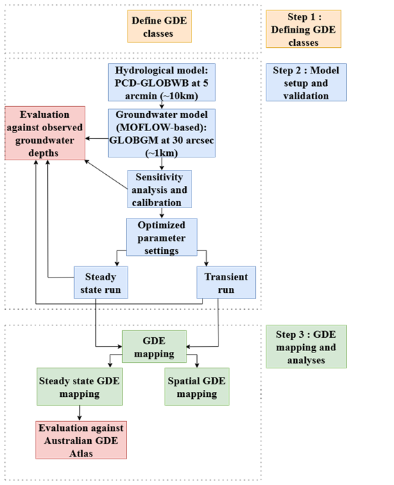
Figure 1 Groundwater-dependent ecosystem (GDE) mapping framework using a high-resolution groundwater model.

2.1 Defining GDE classes (step 1)

We categorize groundwater-dependent ecosystems into three classes based on interaction with groundwater (see Fig. 2). These include (1) ecosystems that depend on sufficient groundwater discharge (aquatic GDEs such as streams and rivers), (2) ecosystems that need shallow groundwater tables and soil saturation (wetland GDEs), and (3) ecosystems that depend on groundwater for root water uptake (terrestrial GDEs with phreatophyte vegetation). In the case of aquatic ecosystems, we do not include lakes due to the complexities in determining the contribution of groundwater in lentic systems, and we exclusively focus on lotic systems – in this case rivers. Also note that we focus on inland ecosystems only. Finally, we do not consider subsurface ecosystems that rely on groundwater, such as stygofauna communities (Huggins et al., 2023), because of the complexity of mapping these communities as previously done by Huggins et al. (2023) as well.

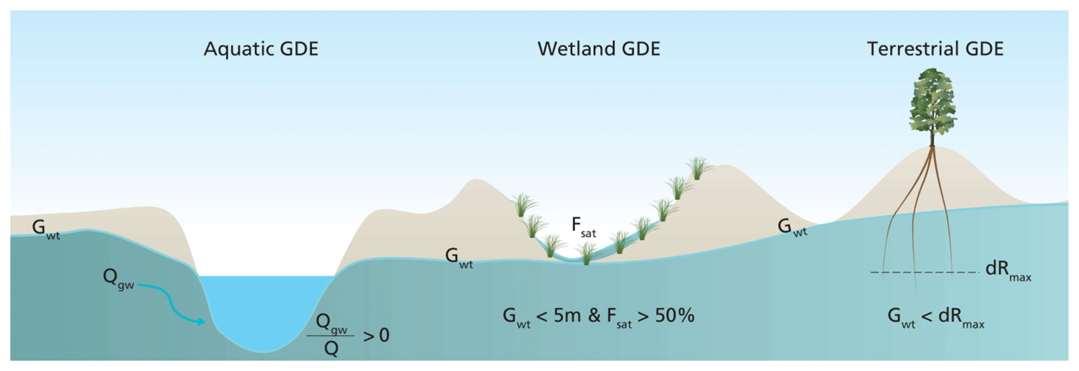
Figure 2 Criteria for defining groundwater-dependent ecosystems, with Q_gw representing local groundwater discharge, Q representing accumulated streamflow, G_wt representing groundwater table depth, F_sat representing saturated area fraction, and dR_max representing maximum rooting depth.

For aquatic GDEs, any stream pixel where the ratio of groundwater discharge (Q_gw) to total streamflow (Q) $\frac{Q_{\text{gw}}}{Q}>\mathrm{0}$ for more than a month is classified as being groundwater dependent. The rationale behind using groundwater discharge as a metric is that it maintains streamflow during dry spells and due to the relatively constant temperature of groundwater, which modulates stream temperatures during warm periods. For terrestrial GDEs (phreatophyte vegetation), we assume that any cell with a vegetation type with maximum rooting depth (D_rmax) less than the groundwater depth of that cell is groundwater dependent, assuming that, in this case, the vegetation is able to access groundwater with its deepest roots during dry spells.

We define wetland GDEs based on the fraction of saturated area (soil wetness) and groundwater level. Any cell that has a saturated area fraction (F_sat) greater than 50 % and a groundwater table depth less than 5 m is classified as a wetland GDE. While groundwater levels closer to the surface (0.5–3 m) support core wetland functions (Eamus et al., 2006; Winter, 1999), wetlands in arid and semi-arid regions can still exhibit groundwater dependence with water table depths up to 5 m, particularly in peripheral or drought-adapted areas (Stromberg et al., 2010). Hence, the threshold of 5 m accommodates both core and peripheral groundwater-supported zones across varied climates. We added the 50 % soil saturation threshold to discern dry areas with shallow groundwater levels from actual wetlands, which are typically saturated at the surface. We performed a sensitivity analysis for varying groundwater depth thresholds (1–5 m) and saturated area fractions (0.1–1.0) with a total of 100 combinations, showing that the threshold of 5 m produces the highest critical success index when validating against the Australian GDE atlas (see Fig. S1 in the Supplement). In the latter case, we assessed the “degree of groundwater dependency” for each GDE type identified on the basis of a monthly time step (Fig. 1).

2.2 Model setup, sensitivity analysis, and output evaluation (step 2)

For this research, we use an integrated hydrological model that consists of two parts. The first part is a physically based global hydrology and water resources model (PCR-GLOBWB version 2.0; Sutanudjaja et al., 2018) that simulates global terrestrial hydrology, including the human impacts (dams and human water use). The second is a time-dependent (transient) groundwater flow model (GLOBGM; Verkaik et al., 2024). The two models are linked through a one-way coupling; that is, the outputs of the PCR-GLOBWB model are used as inputs to the groundwater flow model (Sutanudjaja et al., 2011). We first run PCR-GLOBWB 2 with its own default groundwater parameterization and then use the time series outputs for surface water levels, saturated area fraction, and groundwater recharge as forcing for the groundwater flow model. Model input parameters and data source references as well as groundwater properties for the model can be found in the Supplement (Figs. S2 and S3 and Table S1).

2.2.1 PCR-GLOBWB

PCR-GLOBWB 2 is a gridded integrated hydrology and water resources model with a latitude–longitude grid of 5 arcmin spatial resolution that simulates terrestrial hydrology and human water use at a daily time step. A detailed model description can be found in Sutanudjaja et al. (2018). PCR-GLOBWB 2 is forced with precipitation, temperature, and reference evaporation based on the W5E5 meteorological data set (Cucchi et al., 2020; Lange et al., 2021). Soil parameters are based on the SoilGrids dataset (Hengl et al., 2017). We use the default model settings with four land-cover types, aggregating land cover classes into tall natural vegetation, short natural vegetation, non-paddy irrigated crops, and paddy irrigated crops (Sutanudjaja et al., 2018). To simulate variations in the saturated area fraction, we use the improved ARNO scheme (Todini, 1996; Hagemann and Gates, 2003), which is an integral part of PCR-GLOBWB 2, to assess the area subject to surface runoff. PCR-GLOBWB 2 also has an irrigation and water use model that calculates water demand (Wada et al., 2014) and water withdrawal, water consumption, and return flows for irrigation, domestic, livestock, and industrial sectors.

2.2.2 Groundwater model

We use the two-layer groundwater model GLOBGM run at 30 arcsec (16 million active cells) to simulate groundwater depths, groundwater heads, and groundwater discharge. The model code that is used is MODFLOW 2005, and the aquifer properties are taken directly from de Graaf et al. (2017). The groundwater model is forced with surface water levels and net groundwater recharge (percolation minus capillary rise) over the period 1979–2019 at monthly time steps as obtained from runs with PCR-GLOBWB 2. For net recharge, simple resampling is used, while water levels are computed at 30 arcsec based on a simple routing method of characteristics (for details, see Sutanudjaja et al., 2018) of the 5 arcmin specific discharge over a 30 arcsec drainage network based on HydroSHEDS (Lehner et al., 2008). The steady-state groundwater model is run with average net groundwater recharge and surface water levels over 1979–2019. Subsequently, the transient run follows with the heads from the steady-state run as the initial condition and after a sufficient spinup period of 20 years.

2.2.3 Sensitivity analysis and calibration of groundwater model parameters

With groundwater recharge and boundary conditions as described above, the groundwater model results are possibly sensitive to aquifer transmissivity and storage coefficient, riverbed conductance, and the thickness of the confining layer, while these properties are often very uncertain at larger scales (Brunner et al., 2017). We perform a sensitivity analysis using 216 steady-state simulations by varying the following three parameters: riverbed conductance, vertical conductivity of the confining layer (if present), and transmissivity of the confined and unconfined aquifers. We change these parameters independently using a single prefactor k applied to the log-transformed parameter of concern, with k=1 being the initial value of the parameter taken from de Graaf et al. (2017). See Eq. (1) for an example of the transmissivity:

$$\begin{array}{}\text{(1)}& T^{\prime }=\exp (k\cdot \ln (T\left)\right),\end{array}$$

with T^′ the perturbed transmissivity (m² d⁻¹), T the original transmissivity according to de Graaf et al. (2017), and k the prefactor applied.

For each unique parameter combination, we evaluate the biases between the simulated steady-state groundwater depth (surface elevation minus hydraulic head in the top layer) and time-averaged observed groundwater depths using data from 15 345 wells recorded from 1970 to 2019 at a monthly time step. If there were multiple wells within a 1 km cell, we calculate the average of these considering the same year. We then select the best parameter set with the least bias against observed well data and vary the storage coefficient and conduct six transient runs to select the best parameter set for simulating transient groundwater levels. Based on this, we finally select the best parameter set for the GDE mapping.

2.2.4 Evaluation of simulated groundwater depths

We evaluate the transient simulated groundwater depths against observed groundwater well-depth time series data (Bureau of Meteorology, 2023). We compare 5 million cells with simulated groundwater depths with the observed data from 1979 to 2019 in the Australian continent. The metrics used for evaluation are bias (Baker, 1987), Pearson correlation coefficient (Cohen et al., 2009), and relative variance (Grömping, 2007).

2.3 GDE mapping (step 3)

2.3.1 Steady-state GDE mapping

After running the model in steady-state mode (average forcing groundwater dependent), we map the three different classes of GDEs according to the classification rules described above (Fig. 2). For aquatic GDEs, we derive an aquatic ecosystem dependency ratio to groundwater that is defined as $\frac{Q_{\text{gw}}}{Q}$, where Q_gw is the local groundwater discharge and where Q is the total streamflow.

Wetland GDEs are mapped using the groundwater depth from the groundwater model and the average saturated area (1979–2019) from PCR-GLOBWB 2. Terrestrial vegetation GDEs are mapped using the groundwater depth and a rooting depth map (Fan et al., 2017).

After mapping these GDEs in steady-state mode, we evaluate the results by comparing these with the GDEs mapped by the Australian GDE atlas using similarity index metrics. These metrics are the hit rate h (a class is present that is also mapped), false alarm rate f (a class is mapped that is not present), and miss rate m (a class is present that is not mapped). From these metrics, we also calculate the critical success index (CSI) for the mapping of each GDE type, defined as Eq. (2):

$$\begin{array}{}\text{(2)}& \text{CSI}={\displaystyle \frac{h}{h+f+m}}.\end{array}$$

Note that the Australian GDE atlas distinguished between actually observed GDEs and likely GDEs (Doody et al., 2017), where the latter are mapped based on land-cover type. When evaluating the mapping, we did not distinguish between known and likely GDEs, because of the overall good performance in our mapping approach and similarity in the hit rates between the known and likely GDEs (see Fig. S4 in the Supplement).

2.3.2 Transient GDE mapping

For the transient analysis of the GDEs, we use monthly time series of groundwater depth, groundwater discharge and saturated area fraction from the transient simulation over the period 1979–2019. We use the same criteria for mapping GDEs as used for mapping in steady-state mode and use the extent of the steady-state-mapped GDEs as a given. Within these areas, we consider the temporal variability in the contribution of groundwater. For aquatic GDEs, we use monthly values of $\frac{Q_{\text{gw}}}{Q}$ to classify each month as having a low dependence (ratio<0.25) moderate dependence (ratio between 0.25 and 0.75), or high dependence (ratio>0.75) on groundwater. For terrestrial and wetland GDEs, we record the average number of months per year that the system is classified as groundwater dependent. We separately identify these transient GDE measures for two 20-year periods (1 January 1979 to 31 December 1999 and 1 January 2000 to 1 January 2019) to assess potential changes in the contribution of groundwater between these two time periods.

3 Results

We first present the evaluation of the groundwater model simulations, as a first performance indicator of the proposed GDE mapping methodology (Sect. 3.1). We then evaluate the coincidence of GDE types mapped with the steady-state groundwater model with GDEs mapped by the Australian GDE atlas (Doody et al., 2017) (Sect. 3.2). Finally, we show the temporal change in the degree of groundwater dependency of the different GDE classes based on the transient simulations over the period that is groundwater dependent (Sect. 3.3).

3.1 Performance of the groundwater model in simulating groundwater heads

From the sensitivity analysis and calibration, it turned out that the performance metrics calculated from the groundwater head observations were rather insensitive to the prefactors (see Fig. S5 in the Supplement). We therefore decided to use the default parameters for further analyses. In general, the cumulative frequency distributions show a good agreement in timing (∼75 % shows r>0.25). The dissimilarities between the observed and the simulated heads are due to the bias. Our simulated heads are deeper than the observed ones, with ∼70 % having a bias ranging 0–5 m. Plotting the biases per depth category of the observation data (wells) (Fig. S6 in the Supplement), we observe a smaller bias for shallower depths compared to the deeper depths. This shows that where it matters for GDEs (i.e. shallower depths), the biases are also smaller. The relative variance shows an underestimation of groundwater level variation of ∼80 % with a relative variance <0.6.

The groundwater head of the first layer as simulated with the steady-state groundwater model and the best parameter set from the sensitivity analyses is shown in Fig. S7 in the Supplement, presenting a wide range in groundwater heads over Australia (0.25 to >320 m). Figure S8 in the Supplement shows the differences in simulated (steady-state) groundwater heads for areas where a confining layer is present. The red areas are those where there is a confining layer and the heads in the aquifer underlying the confining layer are larger than those in the confining layer itself. In these areas, it is possible that deep incising surface waters could receive groundwater discharge from the lower aquifer.

Figure 3 shows maps as well as cumulative frequency distributions of the bias (in m; difference in temporal mean heads: simulated minus observed), Pearson correlation coefficient (between the observed and simulated groundwater heads over time), and the relative variance (temporal variance of simulated time series divided by the temporal variance of the observed time series). Note that we compared the simulated groundwater depths from layer 1 with all available observation wells. Due to a lack of data on the well filter depths, we were not able to exclude the wells with filters in confined aquifers. This will likely have a negative effect on model performance. Results show that the evaluation metrics perform better in Tasmania and areas where the wells are likely not in a confined aquifer, i.e. the red areas in Fig. S8 (with r>0.6, bias ≤3 m).

Figure 3 Evaluation statistics of observed groundwater depths against simulated groundwater head; (a–c) maps with values per observed location; (d–f) associated cumulative frequency distributions; (a, d) bias (m); (b, e) Pearson correlation coefficient; (c, f) relative variance. The white areas on the maps are locations without observation data.

3.2 Steady-state mapping and evaluation of GDEs

To map the locations of GDEs, we use the steady-state outputs from our groundwater model. For the aquatic GDEs, we observe that most streams of well-known river basins such as the Darling River depend on groundwater. Some vegetation located in dry areas tap into groundwater levels, while wetlands, showing large ranges in size, depend on groundwater predominantly when located close to rivers, likely being wetlands in or nearby floodplains.

Evaluating our mapped GDEs against the Australian GDE atlas by Doody et al. (2017), we observed high hit rates of 87 %, 92 %, and 95 % for aquatic, terrestrial, and wetland GDEs, respectively (Fig. 4). Despite the overall bias observed in the groundwater model (Fig. 3), the impact on representing GDEs is limited since this bias is smaller for shallower groundwater levels than for deeper groundwater levels (Fig. S6). For the aquatic GDEs, most of the false alarms are in the near-coastal areas and in the Great Artesian Basin. We miss some terrestrial GDEs in western Australia due to a lack of good rooting depth data. We also wrongly identify a large area of wetlands in New South Wales.

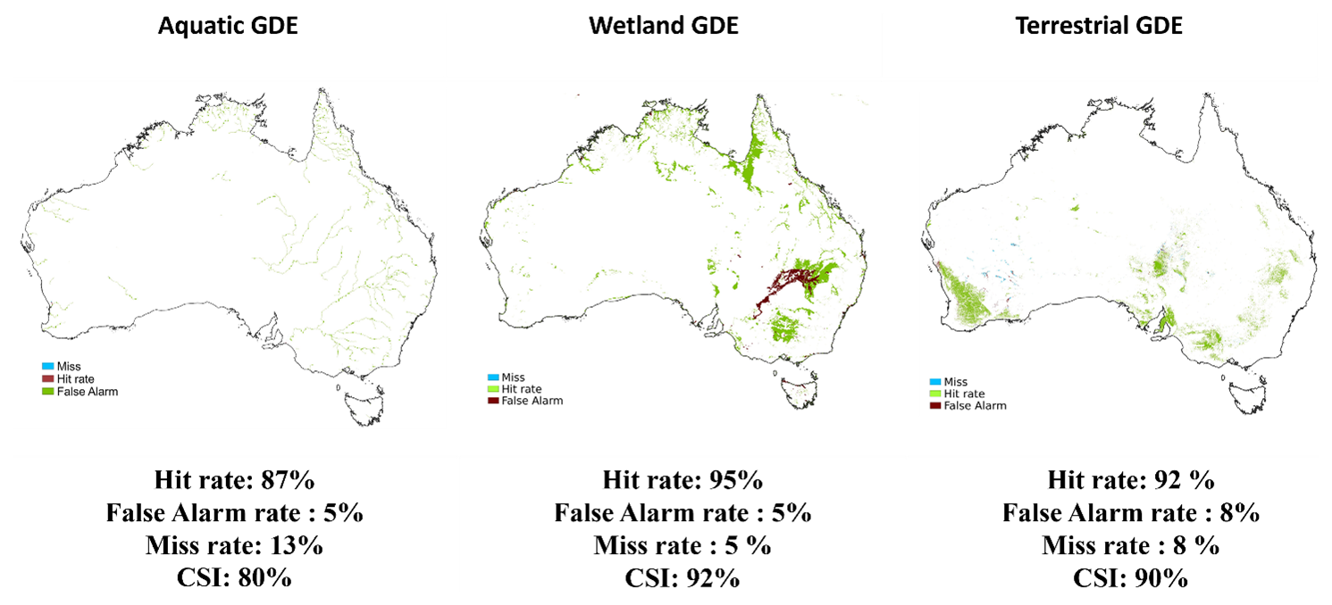
Figure 4 Mapped GDEs based on steady-state groundwater model results evaluated against the Australian GDE atlas showing hit rate, false alarm rate, miss rate, and the CSI for the three GDE classes. Blue colour represents missed ecosystems, dark red represents false alarm, and green represents hit rate.

3.3 Transient GDE mapping

To understand how the contribution of groundwater to the different ecosystems varied in the past, we divided the simulated periods into two time intervals (period 1: 1979–2000; period 2: 2001–2019) and estimated for each time interval the average number of months per year that each GDE type relies on groundwater. Next, we calculated the changes in number of months of groundwater dependency: period 2 minus period 1 (Figs. 5 and 6). We used the mapped steady-state extent as a given for the evaluation of the degree of groundwater influence on GDEs for the transient runs. In other words, we did not look into extent dynamics.

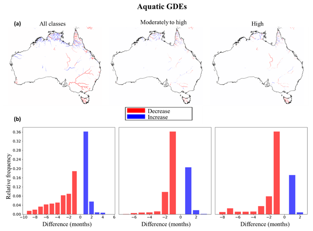
Figure 5 Change in groundwater dependency of aquatic GDEs between 1979–2000 and 2001–2019; (a) maps of the direction of change in the average number of months that aquatic GDEs depend on groundwater; the left panel shows the change in the number of months $\frac{Q_{\text{gw}}}{Q}>\mathrm{0}$ (low to high dependency), the middle panel $\frac{Q_{\text{gw}}}{Q}>\mathrm{0.5}$ (moderate to high dependency), and the right panel $\frac{Q_{\text{gw}}}{Q}>\mathrm{0.75}$ (high dependency); red areas indicate a decrease in the average number of months with groundwater dependency and blue indicates an increase; (b) associated frequency distributions of change in number of months.

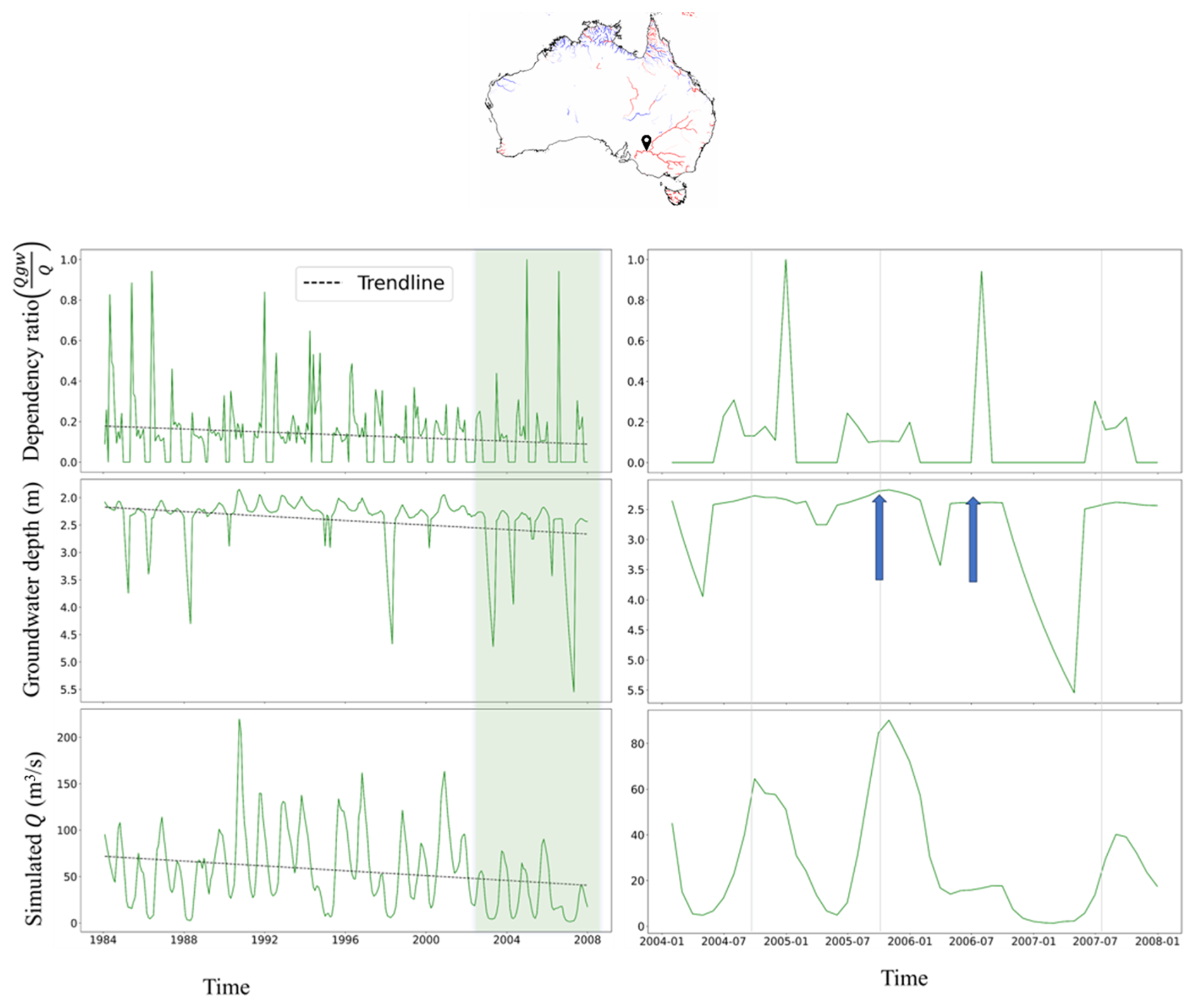
Figure 6 Example time series of $\frac{Q_{\text{gw}}}{Q}$ for a downstream river reach location in the Darling River (location indicated in the aquatic GDE map on top). Top: time series of simulated $\frac{Q_{\text{gw}}}{Q}$, total streamflow (Q), and groundwater depth, including trend lines. Right panels: zoomed-in view into a selected time frame (green bar in the left panels) to show how the variability of dependence of $\frac{Q_{\text{gw}}}{Q}$ depends on groundwater level and streamflow.

For aquatic GDEs, we assessed temporal changes in the different dependency ratio ($\frac{Q_{\text{gw}}}{Q}$) categories. We observe that there is a decline in the average number of months in all dependency classes (Fig. 5) and that the decline in groundwater contribution is mostly observed in streams in the Murray–Darling Basin. This is in accordance with the decline in groundwater levels between the two periods in both the simulations and the observations (Fig. S9 in the Supplement). It is important to realize that the dependency ratio depends on both the groundwater depth and related groundwater discharge (Q_gw) as well as the streamflow itself. This is illustrated in Fig. 6 that shows simulated time series of $\frac{Q_{\text{gw}}}{Q}$, groundwater depth, and total streamflow. The figure shows that the groundwater levels are constrained at the top by the drainage system and also shows the intermittent character of the Australian climate, with wet periods alternating with dry periods where groundwater levels decline and streamflow becomes almost zero. The top figure shows a negative trend in groundwater levels. However, streamflow is also declining, offsetting the decline in groundwater discharge, resulting in a smaller negative trend in groundwater dependency ($\frac{Q_{\text{gw}}}{Q}$). The zoomed-in view at the bottom shows the importance of discharge variability. November 2005 and July 2006 show almost the same shallow water table. However, streamflow peaks in November 2005, which makes for a low dependency ratio, while the 2006 streamflow is low in July, making the dependency on groundwater discharge large.

Figure 7 shows the change in the number of months that the terrestrial GDEs and wetland GDEs are groundwater dependent. For wetland GDEs, we observe a decline in groundwater contribution of on average 4 months per year in most regions, with an exception in some wetland areas in New South Wales and South Australia where an average increase of 8 months of groundwater dependency is observed. For wetland GDEs, this decline can also be caused by a decline of the saturated area fraction, which is a driving factor for the decrease in wetland GDE dependency in central Australia since these areas show only limited declines in groundwater levels. Terrestrial GDEs (phreatophytes) show a limited decline in groundwater dependency of 1 month on average for most locations. These changes are exclusively due to a decline in groundwater levels since the rooting depth is kept constant (see Fig. S7).

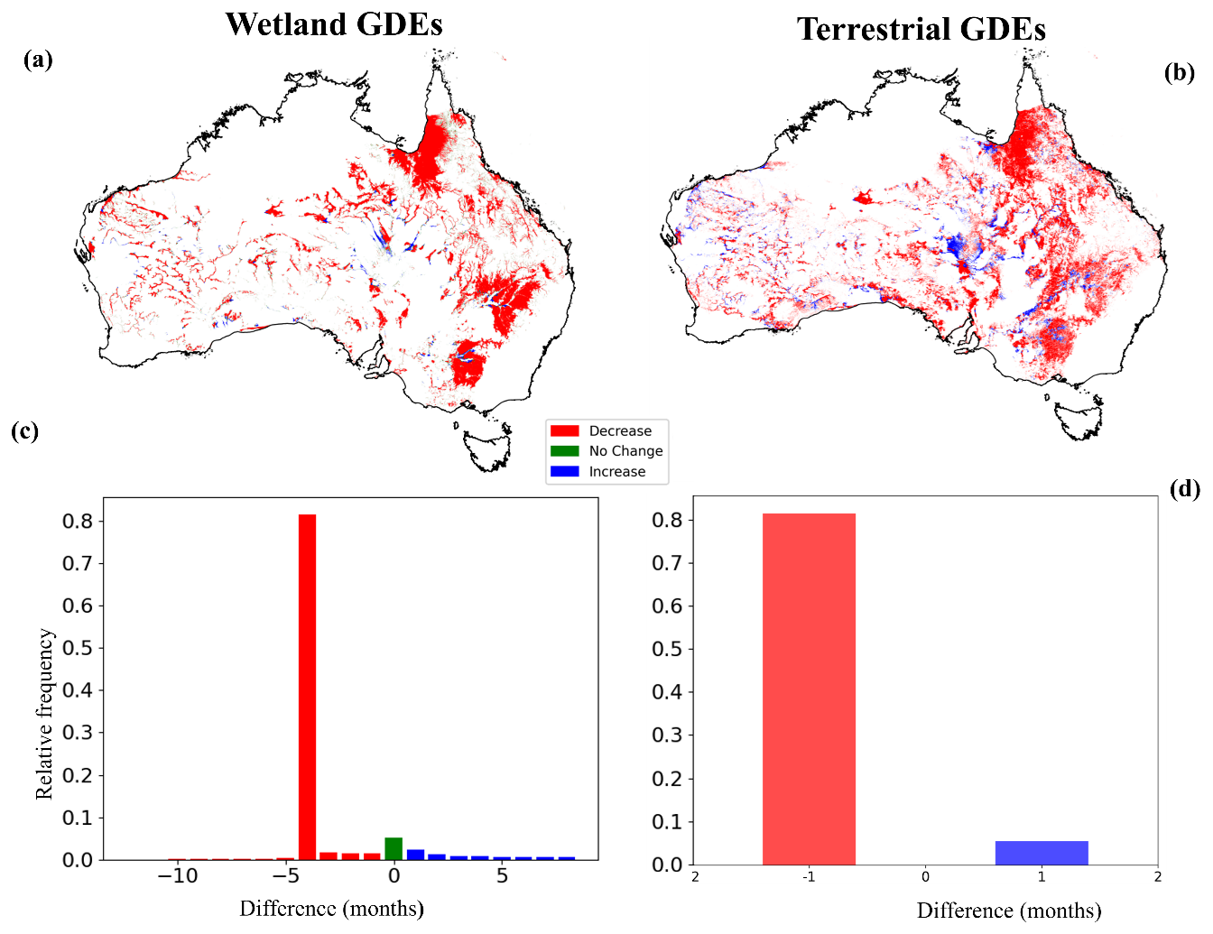
Figure 7 Change in average number of months of groundwater the dependency of terrestrial GDEs (phreatophytes) and wetland GDEs; (a) direction of change in terrestrial GDEs (phreatophytes); (b) direction of change in wetland GDEs. Red areas indicate a decrease in the average number of months with groundwater dependency, green indicates no change between the periods, and blue indicates an increase; (c, d) associated cumulative frequency distributions of change in number of months.

We have performed some additional analyses to provide insight into the drivers of groundwater level changes between both periods. Figure S10 in the Supplement shows the difference in simulated groundwater recharge between the periods 2001–2019 relative to 1979–2000 and the simulated groundwater withdrawal over the 2001–2019 period. The changes in groundwater recharge reflect the impact of climate variability and/or change on the groundwater system, while the locations with groundwater withdrawal reflect the direct human impacts. A thorough factor analysis is beyond the scope of this study, but a comparison of Figs. 7 with S9 suggests that climate variability mainly explains the changes in groundwater depth in north, central, and western Australia, while both factors play a role in eastern Australia. Note that the variability of the simulated groundwater levels is half of that of the observed ones. This reflects the underestimation of the variability in groundwater depth as shown in Fig. 3. Possible explanations for this are an underestimation of recharge and recharge variability in drylands (Quichimbo et al., 2021), an overestimation of storage coefficients, and an underestimation of groundwater withdrawals.

4 Discussions and conclusions

In this research, we developed and evaluated a framework using a surface–groundwater model at 30 arcsec resolution to map aquatic, wetland, and terrestrial groundwater-dependent ecosystems. We evaluated the simulated groundwater heads with observed groundwater level observations and the mapped GDE occurrence with the GDE atlas of Australia. Groundwater resources are crucial for GDEs as they partially or fully contribute to their water budget. Analysing the spatial and temporal changes in groundwater dependency is required for understanding threats to GDEs. In the context of global population growth, industrialization, economic growth, and climate change driving global groundwater depletion, this will inform relevant stakeholders on threatened ecosystems and direct groundwater allocation. This study introduces a method for GDE mapping that offers the possibility to improve understanding of the spatial distribution and temporal dynamics of GDEs in relation to the spatio-temporal dynamics of groundwater systems.

Our research complements previous work on mapping GDEs combining expert knowledge, GIS and field visits by Doody et al. (2017); previous global groundwater modelling efforts (de Graaf et al., 2019); and work by Eamus et al. (2015), who investigated GDE responses to changes in groundwater depth using satellite images and field studies for selected locations. In comparison, our research proposes a methodology to understand the long-term temporal responses of different GDE types to changes in groundwater levels at a large spatial extent and at high resolution. Our method relies on outputs from a process-based high-resolution large-scale groundwater model and has potential for identifying hotspots of ecosystems threatened by groundwater extractions on a large scale. It proved to be effective for identifying GDEs in Australia with a hit rate over 87 % and CSI over 80 %. GDEs occur in areas with a shallow water table, and, notably, our framework was well able to simulate groundwater depths at these locations. The transient component of this methodology also facilitates in-depth understanding of the temporal dynamics of the reliance on groundwater resources by GDEs. At a monthly timescale, we were able to simulate the different levels of dependency by aquatic GDEs as well as the levels of reliance or non-reliance on groundwater resources by wetlands and phreatophyte communities.

It is important to note that the dependency ratio of aquatic GDEs is dependent on both total streamflow and groundwater depth. Thus, increased groundwater discharge coupled with a decrease in streamflow may shift a river section to be more dependent and vice versa. Although streamflow and groundwater levels are likely positively correlated at larger timescales, they may not be in phase at shorter timescales due to the different response times of surface water and groundwater systems. This makes the degree of groundwater dependency of aquatic GDEs more intermittent when compared to GDEs that rely on groundwater depth and soil wetness (wetlands) or groundwater depth only (phreatophyte communities). Phreatophytes may be even more resilient to change as they are able to adapt to groundwater level declines through deeper rooting (Naumburg et al., 2005), although there are limitations to this adaptive capacity between species, implying that a decline in groundwater level may result in changes in phreatophyte community composition (Sommer and Froend, 2014).

The model performance evaluation in the transient analysis revealed a fair overall agreement between simulated and observed groundwater head data yet also an overall overestimation in simulated groundwater depth. However, since biases for shallow groundwater levels were limited, the performance in identifying the GDEs was very good, as indicated by the different performance metrics. The calibration results show that the groundwater model was not very sensitive to global changes in parameter sets (Fig. S5). This calls for more sophisticated groundwater calibration methods that allow for regional differentiation in model parameters. Also, further improvements can be expected if the recharge simulated with PCR-GLOBWB 2 could be better constrained. Therefore, a calibration approach more sophisticated than prefactor parameter change must be implemented to improve the groundwater model simulations and derived mapping of GDEs.

One of the limitations of the current groundwater model setup is its relatively simple hydrogeologic schematization obtained from de Graaf et al. (2017). Although this makes the framework globally applicable, it may suffer from a lack of geological detail needed for representing groundwater discharge and springs over, for example, the Great Artesian Basin. Another limitation is the assumption that the rooting depth of phreatophytes is constant, due to a lack of temporal rooting depth data. This assumption contrasts with studies that have shown the ability of plants to adapt to changes in groundwater levels (Fan et al., 2017; Robinson, 1958).

Although we noted a decline in groundwater contribution to Australian GDEs over the past decades, we have not explicitly factored in potential impacts from climate change or unsustainable groundwater extraction on GDE extent. Also, we cannot conclude on GDE loss solely from our findings, as we have not observed a consistent lack of groundwater contribution throughout the year. The potential underestimation of groundwater level changes (Fig. S9) and withdrawals at a high resolution (Fig. S10) in our simulations could be a contributing factor.

In future work, we intend to apply our framework to the global scale and better assess the individual impacts of groundwater withdrawals and climate change on the extent of GDEs under different scenarios. This would also require us to translate the change in degree of groundwater contribution to a change in GDE extent. This work will be accompanied by improved hydrogeological schematization and better calibration methods, with the aim to provide a good basis for ecological assessments, where changes in GDE extent are linked to changes in species richness.

In summary, the framework introduced in this study represents a GDE mapping approach that allows for the assessment of spatio-temporal dynamics associated with the dependency of ecosystems on groundwater resources. This generic methodological framework not only enhances our understanding of the spatial distribution of GDEs but also establishes a foundation for interdisciplinary research between ecology and hydrology. By offering a global perspective on hotspot areas of GDEs under various hydroclimatic conditions, this methodology can inform decision-making processes regarding groundwater allocation and species conservation efforts. Such initiatives are crucial for advancing the objectives outlined in, for example, the Kunming-Montreal Global Biodiversity Framework and Sustainable Development Goal 15, which aims to halt biodiversity loss.