Technical note: What does the Standardized Streamflow Index actually reflect? Insights and implications for hydrological drought analysis

Hydrological drought is one of the main hydroclimatic hazards worldwide, affecting water availability, ecosystems, and socioeconomic activities. This phenomenon is commonly characterized by the Standardized Streamflow Index (SSI), which is widely used because of its straightforward formulation and calculation. Nevertheless, there is limited understanding of what the SSI actually reveals about how climate anomalies propagate through the terrestrial water cycle. To find possible explanations, we implemented the Structure for Unifying Multiple Modeling Alternatives (SUMMA) coupled with the mizuRoute routing model in six hydroclimatically different case study basins located on the western slopes of the extratropical Andes and examined correlations between the SSI (computed from the models for 1-, 3-, and 6-month timescales) and potential explanatory variables – including precipitation and simulated catchment-scale storages – aggregated at different timescales. Additionally, we analyzed the impacts of adopting commonly used timescales on propagation analyses of specific drought events – from meteorological to soil moisture and hydrological drought – with focus on their duration and intensity. The results reveal that the choice of timescale for the SSI has larger effects on correlations with explanatory variables in rainfall-dominated regimes compared to snowmelt-driven basins, especially when simulated fluxes and storages are aggregated to timescales longer than 9 months. In all the basins analyzed, the strongest relationships (Spearman rank correlation values over 0.7) were obtained when using 6-month timescales to compute the SSI and 9–12 months to compute the explanatory variables, excepting aquifer storage in snowmelt-driven basins. Finally, the results show that the trajectories of drought propagation obtained with the Standardized Precipitation Index (SPI), the Standardized Soil Moisture Index (SSMI), and the SSI may change drastically with the selection of timescale. Overall, this study highlights the need for caution when selecting standardized drought indices and associated timescales, since their choice impacts event characterizations, monitoring, and propagation analyses.

1 Introduction

Droughts are natural hazards that can cover vast areas over a period of months to several years (Samaniego et al., 2013; Brunner and Tallaksen, 2019), with large effects on environmental systems (Vicente-Serrano et al., 2020) and socioeconomic activities (Wilhite and Pulwarty, 2017). These events are primarily triggered by precipitation deficits (McKee et al., 1993), which may be associated with internal climate variability modes, such as the El Niño–Southern Oscillation (Okumura et al., 2017; Steiger et al., 2021), and exacerbated by land–atmosphere interactions (Schumacher et al., 2022). Given the warming trends projected for the next decades (e.g., Brunner et al., 2020; Tokarska et al., 2020) and the contribution of higher temperature to drying (Trenberth et al., 2014), anthropogenic climate change is also expected to affect drought characteristics, increasing their frequency, severity, and duration in many regions of the world (Cook et al., 2014; Pokhrel et al., 2021).

Despite the drought concept referring to the notion of below-average water fluxes and/or storages (Tallaksen and Van Lanen, 2004), there are several drought definitions and classifications, with meteorological, agricultural (also referred to as soil moisture drought; e.g., Thober et al., 2015; Cook et al., 2018), hydrological, and socioeconomic being the most used drought types (Wilhite and Glantz, 1985). Among these, hydrological droughts – associated with abnormally low levels in surface water bodies, groundwater, and/or streamflow in rivers (Van Loon, 2015) – are especially relevant due to their direct impacts on natural ecosystems and human society. Hence, understanding how climate anomalies propagate through the terrestrial water cycle to trigger hydrological droughts of different characteristics (e.g., duration, severity) is an outstanding challenge for the scientific community and a crucial task for water resource planning and management (Zhang et al., 2022).

Hydrological droughts are typically quantified through indices derived from observed or modeled time series of streamflow (e.g., Zhu et al., 2016; Stahl et al., 2020), runoff (Shukla and Wood, 2008), and groundwater levels (e.g., Bachmair et al., 2015). Among the existing indices, the Standardized Streamflow Index (SSI; Modarres, 2007; Vicente-Serrano et al., 2012) has become increasingly popular because of its straightforward formulation, calculation, and interpretability for the characterization of discharge anomalies. The numerous SSI applications span various areas, including drought monitoring (Núñez et al., 2014; Nkiaka et al., 2017) and forecasting (Sutanto and Van Lanen, 2021, 2022; Hameed et al., 2023) and drought propagation under historically observed (e.g., Barker et al., 2016; Bhardwaj et al., 2020) and projected (Wan et al., 2018; Adeyeri et al., 2023) climatic conditions.

The applicability of the SSI is challenged by its sensitivity to the quantity and quality of the data (Wu et al., 2018) and the calculation method, which entails the choice of a reference period for standardization, the selection of probability distribution (e.g., Laimighofer and Laaha, 2022; Teutschbein et al., 2022), the parameter estimation approach (e.g., Tijdeman et al., 2020), and, in particular, the timescale or accumulation (e.g., Barker et al., 2016; Baez-Villanueva et al., 2024). The latter refers to the backward-looking period (commonly a number of months) over which streamflow values are averaged before computing the index. Most drought propagation analyses seek possible relationships between meteorological drought indices, such as the Standardized Precipitation Index (SPI; McKee et al., 1993); the Standardized Precipitation Evapotranspiration Index (SPEI; Vicente-Serrano et al., 2010), computed for various timescales; and the SSI, computed for some timescale, with 1 month (SSI-1) being the common choice (e.g., Huang et al., 2017; Peña-Gallardo et al., 2019; Stahl et al., 2020; Wang et al., 2020; Wu et al., 2022; Zhang et al., 2022; Odongo et al., 2023; Baez-Villanueva et al., 2024). Such a decision commonly relies on the assumption that streamflow already includes hydro-meteorological processes of the previous months (e.g., Stahl et al., 2020; Tijdeman et al., 2020; Sutanto and Van Lanen, 2021), enabling direct comparisons with them (e.g., Baez-Villanueva et al., 2024). Because SSI-1 may be susceptible to short-term fluctuations, other authors have preferred smoothed (e.g., 3-month averages) time series of SSI-1 (e.g., Bhardwaj et al., 2020): 3-month (e.g., Núñez et al., 2014; Wu et al., 2017; Rivera et al., 2021; Adeyeri et al., 2023; Yun et al., 2023), 6-month (e.g., Seibert et al., 2017; Oertel et al., 2020), or even longer (e.g., Teutschbein et al., 2022; Fowé et al., 2023) timescales.

Nowadays, there is no consensus regarding the most appropriate timescale for both SSI and possible explanatory variables (e.g., precipitation and catchment-scale simulated storages), which may stem from the limited understanding of what the SSI truly reveals about the underlying physical mechanisms driving hydrological droughts. For example, Buitink et al. (2021) examined five components of the water cycle – precipitation, soil moisture, vegetation greenness, groundwater, and surface water – in the Dutch province of Gelderland, finding that percentile-based thresholds commonly used for hydrological drought detection mask out more frequent drought conditions that other variables in the system may be experiencing.

To tackle this issue, process-based hydrological modeling arises as a useful approach (Peters-Lidard et al., 2021), and the literature is rich in studies using models with varying degrees of complexity to examine the propagation from meteorological to soil moisture or hydrological droughts (e.g., Andreadis et al., 2005; Sheffield and Wood, 2007; Van Loon and Van Lanen, 2012; Samaniego et al., 2013; Van Loon et al., 2014; Zink et al., 2016; Apurv et al., 2017; Bhardwaj et al., 2020; Lee et al., 2022; Rakovec et al., 2022). This paper contributes to this field by combining observed data and a state-of-the-art physics-based modeling framework to analyze fluctuations in the widely used SSI across hydrological regimes. Here, we depart from previous hydrological drought assessments that used a unique timescale for the SSI (e.g., Stahl et al., 2020; Tijdeman et al., 2020; Wu et al., 2022; Baez-Villanueva et al., 2024) by conducting exploratory correlation analyses between modeled catchment-scale water storages and the SSI to subsequently inform the choice of timescales for the calculation of standardized indices (e.g., Samaniego et al., 2013) and drought propagation analyses. Specifically, we address the following research questions:

1. How do different timescales affect the number and duration of hydrological droughts?

2. How does the SSI relate to catchment-scale water storages and fluxes across different hydrological regimes?

3. How do different timescales affect the propagation of historically observed meteorological droughts toward soil moisture and hydrological droughts?

To seek answers, we configure the Structure for Unifying Multiple Modeling Alternatives (SUMMA; Clark et al., 2015a, b, 2021) hydrological model and the vector-based routing model mizuRoute (Mizukami et al., 2016, 2021) in six basins located along the western slopes of the extratropical Chilean Andes. Catchment-scale precipitation and model simulations are temporally aggregated to monthly time steps to compute snow water equivalent (SWE), soil moisture, aquifer storage, total storage (i.e., the sum of SWE, soil moisture, aquifer storage, and canopy storage), and the SSI for different timescales. We use these time series to explore the physical processes explaining variations in the SSI during the period April 1983–March 2020, along with the drought event of 1998/99 and the recent central Chile megadrought (Garreaud et al., 2017, 2019). Finally, we examine the implications of timescale selection on the portrayal of drought propagation across the duration–intensity space, using standardized indices during historically observed events. We stress that it is not our intention to select or establish the most suitable timescale to be applied in each particular case; instead, we seek to improve the current understanding of the information content of the SSI across different hydrological regimes and raise awareness on the impact that the subjective choice of the timescale and the analysis periods may have on the interpretation and application of the SSI for drought monitoring and propagation analyses.

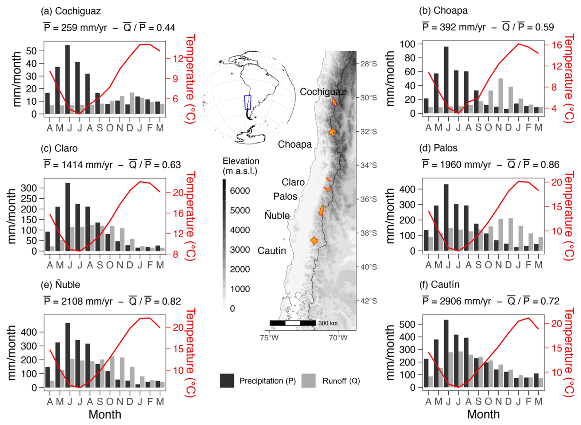
Figure 1 Location, delimitation (orange area in map), and seasonality of precipitation (P), runoff (Q), and temperature for the six case study basins: (a) Cochiguaz River at El Peñón, (b) Choapa River at Cuncumén, (c) Claro River at El Valle, (d) Palos River at Colorado, (e) Ñuble River at La Punilla, and (f) Cautín River at Rari-Ruca. Overlines represent annual averages for the period April 1985–March 2015.

2 Study area and data

2.1 Case study basins

We conduct our analyses in six Chilean basins located on the western slopes of the extratropical Andes Cordillera (Fig. 1): (i) Cochiguaz River at El Peñón, (ii) Choapa River at Cuncumén, (iii) Claro River at El Valle, (iv) Palos River at Colorado, (v) Ñuble River at La Punilla, and (vi) Cautín River at Rari-Ruca. Hereafter, we refer to each basin using the name of the river. The catchment boundaries and the identification number (ID) are obtained from the CAMELS-CL database (Alvarez-Garreton et al., 2018). All the basins receive most of the precipitation during the fall (MAM) and winter (JJA) seasons (Fig. 1). Additionally, the basins span a wide range of physiographic characteristics and climatic conditions, with annual precipitation amounts ranging from 260 to 2900 mm yr⁻¹, mean annual temperatures between 9 and 16 °C, annual runoff spanning 114–2090 mm yr⁻¹, and aridity indices between 0.4 and 3 (Table 1). Such climatic diversity translates into different hydrological regimes: the Cochiguaz and Choapa are snowmelt-driven, Palos and Ñuble have a mixed regime, and Claro and Cautín are mostly rainfall-driven.

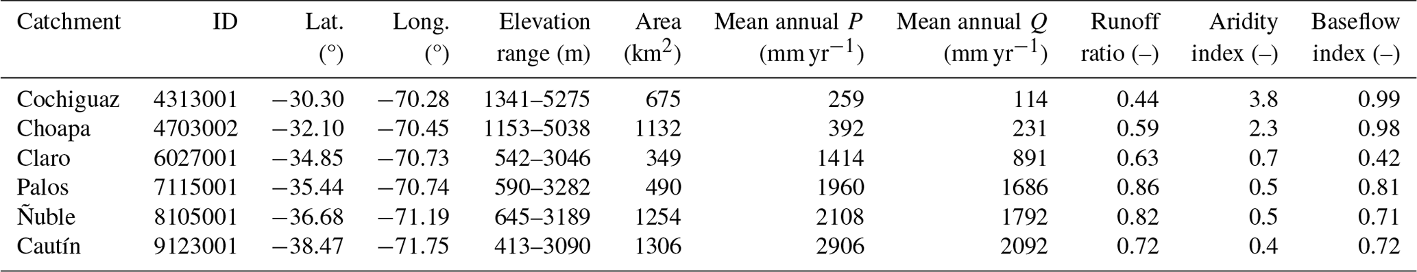
Table 1 Physiographic and climatic attributes of the six basins considered in this study. All data come from the CAMELS-CL database, except for the baseflow index, which was estimated from hydrological simulations in the SUMMA model. The aridity index was calculated as PET/P.

2.2 Datasets

Meteorological daily data are obtained from the CR2MET v.2.0 observational product (DGA, 2017; Boisier et al., 2018), which provides precipitation and extreme temperature estimates for the period 1979–2020 at a 0.05° × 0.05° horizontal resolution. CR2MET precipitation estimations are obtained through multiple linear regression models that consider physiographic attributes and large-scale climate variables from the fifth generation of the ECMWF reanalysis (ERA5; Hersbach et al., 2020) as predictors and observed daily precipitation from gauge stations as predictands. For extreme daily temperatures, CR2MET includes land surface temperature from the Moderate Resolution Imaging Spectroradiometer (MODIS) as a potential explanatory variable. Wind, incoming shortwave radiation, atmospheric pressure, and relative humidity are obtained from ERA5-Land (Muñoz-Sabater et al., 2021). Land cover data and vegetation types for the study area are also obtained from MODIS. Daily streamflow records are collected by the Chilean Water Directorate (DGA) and were retrieved from the website of the Center for Climate and Resilience Research (CR2; https://www.cr2.cl/datos-de-caudales/, last access: 18 September 2023). Table 2 provides a summary of the datasets used in this study, including their horizontal and temporal resolutions.

Table 2 Datasets used in this study.

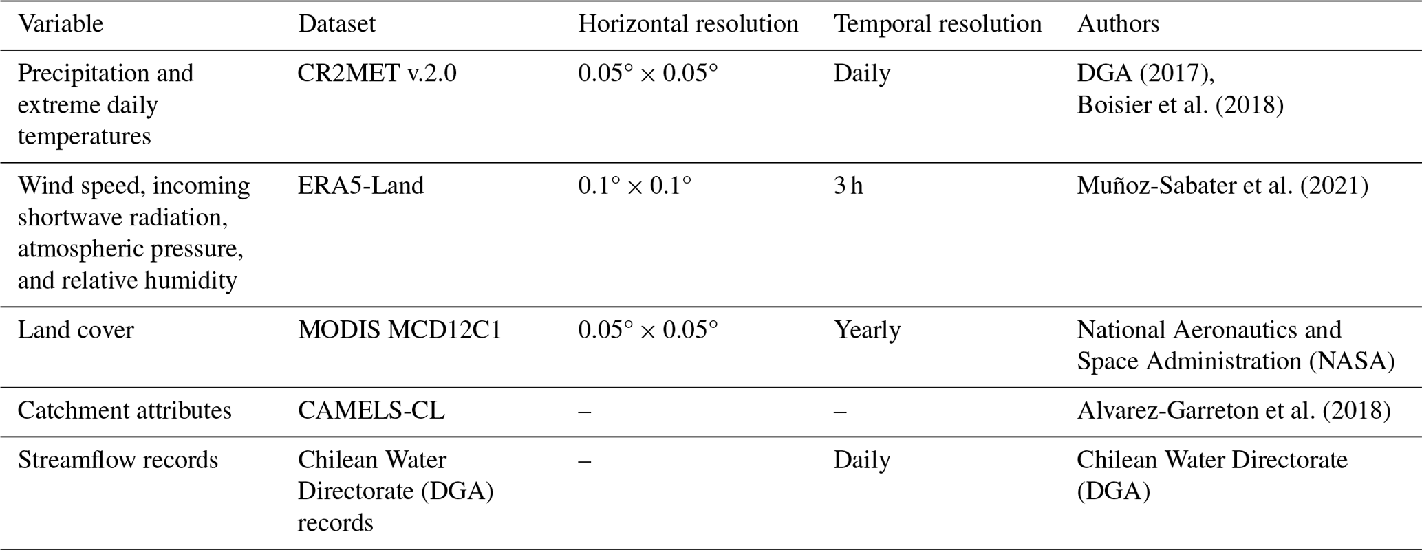
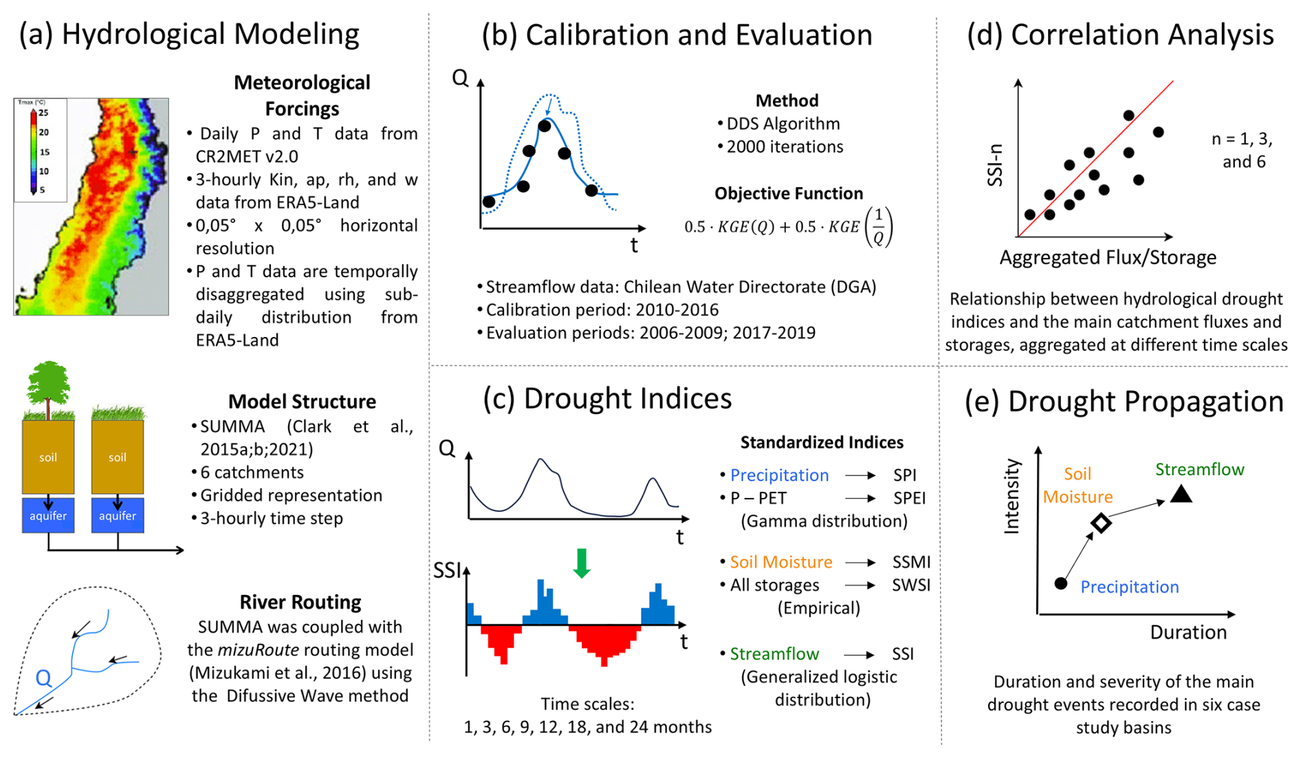
Figure 2 Flowchart describing the approach used in this study, including (a) meteorological forcings, hydrological model structure, and river routing configuration (Sect. 3.1); (b) calibration and evaluation of hydrological models (Sect. 3.2); (c) calculation of drought indices at different timescales and implications for hydrological drought characteristics (Sect. 3.3); (d) correlation analysis between standardized drought indices and aggregated fluxes/storages (Sect. 3.4); and (e) drought propagation analysis (Sect. 3.5). The abbreviations/acronyms used in the figure are as follows. P: precipitation; T: air temperature; Kin: incoming shortwave radiation; ap: atmospheric pressure; rh: relative humidity; w: wind speed; SPI: Standardized Precipitation Index; SPEI: Standardized Precipitation and Evapotranspiration Index; SSMI: Standardized Soil Moisture Index; SWSI: Standardized Water Storage Index; SSI: Standardized Streamflow Index.

3 Approach

Our approach considers the configuration of the SUMMA hydrological model (Clark et al., 2015a, b, 2021) and the mizuRoute routing model (Mizukami et al., 2016, 2021, Fig. 2a); the calibration and evaluation of the SUMMA model parameters (Fig. 2b); the computation of standardized drought indices (SDIs) for precipitation, simulated soil moisture and simulated streamflow, and the examination of timescale effects on hydrological drought frequency and duration (Fig. 2c, Sect. 3.3); and correlation analysis between the SSI and other simulated hydrological variables (Fig. 2d). Finally, we examine how timescales typically adopted for the calculation of standardized indices affect the portrayal of historically observed drought events (Fig. 2e); specifically, we analyze the transitions from meteorological to soil moisture and hydrological droughts in the duration–intensity space (Sect. 3.5). In this paper, we use the terms “timescale” or “temporal scale” when referring to the temporal window used to aggregate (or average) monthly values. For example, the 3-month timescale for September 2015 precipitation is the aggregation of monthly amounts (in mm per month) for July to September 2015. For the case of state variables (e.g., SWE, soil moisture) or fluxes (e.g., streamflow), the 3-month timescale is obtained by averaging monthly means.

A key aspect of our methodology is the identification of hydrological variables and timescales driving fluctuations in the SSI, obtaining all the data from a calibrated, state-of-the-art process-based hydrological model. This approach departs from previous efforts searching for statistical relationships between the SSI – computed with streamflow observations – and standardized indices such as the Standardized Precipitation Index (SPI; e.g., Barker et al., 2016; Huang et al., 2017; Wu et al., 2022), the Standardized Precipitation Evapotranspiration Index (SPEI; e.g., Peña-Gallardo et al., 2019; Wang et al., 2020; Bevacqua et al., 2021), and the Standardized Soil Moisture Index (SSMI; Carrão et al., 2013) or other indices and state variables (e.g., soil moisture, aquifer storage, SWE, total water storage) derived from reanalysis datasets that do not necessarily correspond to observed streamflow anomalies (e.g., Hoffmann et al., 2020; Baez-Villanueva et al., 2024).

3.1 Hydrological modeling

We use the SUMMA hydrologic modeling system, which offers different implementations for a wide range of modeling decisions. In order to force numerical simulations at 3-hourly time steps, daily precipitation and temperature data from CR2MET are temporally disaggregated using the sub-daily distribution provided by ERA5-Land (Muñoz-Sabater et al., 2021). Longwave radiation is computed using the formulation proposed by Iziomon et al. (2003), and the remaining variables are directly obtained from ERA5-Land.

SUMMA has several options for model configuration, process representations, and flux parameterizations for mass and energy balance equations. Here, we used the Jarvis (1976) function for simulating stomatal resistance, one of the main physiological factors controlling transpiration, similar to the Noah-MP land surface model (Niu et al., 2011). We also considered a logarithmic wind profile below the vegetation canopy, described in Mahat et al. (2013), and implemented the Raupach (1994) parameterization for vegetation roughness length and displacement height. We use Beer's law (Mahat and Tarboton, 2012) – as implemented in the Variable Infiltration Capacity (VIC) model (Liang et al., 1994) – to represent the radiation transmission through vegetation. For the vertical redistribution of water along the soil column, we consider the mixed form of the Richards equation (Celia et al., 1990), a vertically constant hydraulic conductivity, and a lumped aquifer model. For snow, we consider a constant albedo decay rate, and the thermal conductivity was parameterized using the Jordan (1991) approach.

In this study, each basin is spatially discretized into grid cells that are delineated to match the meteorological forcing data resolution (0.05° × 0.05°). Each grid cell has specific physiographic characteristics (e.g., slope, elevation, layer thickness, vegetation, and soil type), a maximum of five snow layers, and three soil layers with different thicknesses – top: 0.5 m; middle: 2 m; bottom: 2.5 m. Furthermore, each grid cell incorporates an unconfined aquifer at the bottom of the soil column, which contributes to baseflow generation (Fig. 2a). We stress that no lateral water fluxes are allowed between grid cells.

We use the vector-based routing model mizuRoute (Mizukami et al., 2016, 2021) to convert the instantaneous runoff obtained with the SUMMA model at each grid cell into streamflow at the basin outlet. The application of mizuRoute requires delineating a digital river network, with individual subcatchments contributing runoff to each river reach. Firstly, the model converts the total runoff from each grid cell into subcatchment-scale runoff using area-weighted averages. Then, the model performs a hillslope routing to delay instantaneous total runoff from the subcatchment to the corresponding outlet using a gamma-distribution-based unit hydrograph and then routes the delayed runoff for each river reach in the order defined by the river network topology. Full descriptions of the hillslope routing, general routing procedures, and routing schemes are provided by Mizukami et al. (2016). Here, we use the diffusive wave routing scheme described and implemented by Cortés-Salazar et al. (2023).

3.2 Model calibration and evaluation

We calibrated 14 parameters (Table S1 in the Supplement) of the SUMMA model using the dynamically dimensioned search (DDS) algorithm (Tolson and Shoemaker, 2007), implemented in OSTRICH (Matott, 2017), to maximize the objective function (OF) proposed by Garcia et al. (2017), which provides a good compromise for achieving good high-flow and low-flow simulations:

$$\begin{array}{}\text{(1)}& \text{OF}=\mathrm{0.5}\cdot \text{KGE}\left(Q\right)+\mathrm{0.5}\cdot \text{KGE}\left(\mathrm{1}/Q\right),\end{array}$$

where KGE is the Kling–Gupta efficiency (Gupta et al., 2009) computed with simulated and observed daily time series of Q and $\mathrm{1}/Q$. We set a number of 2000 iterations, which is similar to the number of evaluations used in previous studies (e.g., Rakovec et al., 2016; Shen et al., 2022), and only one optimization trial. The observed daily streamflow data are split into a warm-up period (April 2004–March 2006), a calibration period (April 2010–March 2017), and two non-consecutive evaluation periods (April 2006–March 2010 and April 2017–March 2020). For model evaluation, we use the OF, the KGE, the Nash–Sutcliffe efficiency (NSE; Nash and Sutcliffe, 1970), the coefficient of determination (R²), and the root-mean-square error (RMSE; Fig. 2b).

3.3 Drought indices

For meteorological drought characterization, we use the well-known SPI (McKee et al., 1993), which compares the cumulative precipitation for a specific reference period with its long-term (usually 30 years or more) distribution at a given location. The SPI calculation involves (i) selecting a probability density function (PDF) and its parameters to obtain the reference long-term distribution for cumulative precipitation; (ii) obtaining the cumulative distribution function (CDF) from the fitted distribution; and (iii) transforming the CDF into a standardized normal distribution (i.e. with mean equal to zero and standard deviations of 1), using an equi-percentile inverse transformation to derive the SPI values. Here, we use the parametric gamma distribution (McKee et al., 1993; Stagge et al., 2015) and the probability-weighted moments method (Hosking, 1986) to estimate the parameters in SPI calculations. We also use the SPEI (Vicente-Serrano et al., 2010), which requires monthly precipitation and temperature data and involves a mass balance given by the difference between precipitation and potential evapotranspiration (PET) estimated with the Thornthwaite (1948) equation.

For soil moisture drought analysis, we use the SSMI (Carrão et al., 2013), which quantifies deficits in the soil water content in the root zone relative to its seasonal climatology at a specific location. The SSMI uses an empirical distribution based on monthly soil moisture series. Since the SUMMA model provides other storages besides soil moisture, we also use a modified version – the Standardized Water Storage Index (SWSI) – to assess total water storage (i.e., the sum of SWE, canopy storage, soil moisture, and aquifer storage). Finally, we use the Standardized Streamflow Index (SSI; Vicente-Serrano et al., 2012) for hydrological drought characterization. Here, we use the generalized logistic distribution to compute the SSI, following recommendations from past studies (e.g., Vicente-Serrano et al., 2012; Tijdeman et al., 2020).

To evaluate how the subjective choice of timescales may affect the characterization of different types of droughts and inter-relationships, we compute SDI-n with n=1, 3, 6, 9, 12, 18, and 24 months (Fig. 2c), except the SSI, for which we consider temporal scales that have commonly been adopted under different assumptions and considerations (e.g., Núñez et al., 2014; Oertel et al., 2020; Tijdeman et al., 2020; Baez-Villanueva et al., 2024; see Sect. 3.4). We use the calibrated parameters (see Sect. 3.2) to perform hydrologic model simulations for the historical period April 1981–March 2020. All SDI computations consider a spin-up period of 2 years (April 1981–March 1983) and the same reference period of 30 years (April 1983–March 2013). We further examine how different drought detection criteria may alter the frequency and intensity of hydrological drought events during the historical period. To this end, we apply a fixed-threshold criterion (Van Loon, 2015), set here as −1, in two different ways: (i) a drought event starts when SDI-n drops below −1 and ends when it reaches or exceeds −1 (i.e., it is possible to detect 1-month events, or “free” criteria), and (ii) a drought event begins when SDI-n remains below −1 for at least 3 consecutive months and concludes when it reaches or exceeds −1 (“constrained” criteria).

3.4 Correlation analysis

To understand temporal fluctuations in the SSI, we compute the Spearman's rank correlation coefficient between SSI-n with n=1, 3, and 6 months, which are the most commonly used temporal scales in drought propagation analyses (e.g., Núñez et al., 2014; Oertel et al., 2020), and the main catchment-scale water fluxes and storages as explanatory variables (Fig. 2d), including precipitation, SWE, soil moisture, aquifer storage, and the total water storage in the basin (i.e., the sum of SWE, canopy storage, soil moisture, and aquifer storage). To assess what timescales of the hydrological variables are important for drought occurrence, we use temporal averages or accumulations over the preceding months of 1, 3, 6, 9. 12, 18, and 24 (including the target month). In this analysis, we assume that the factors not simulated by the hydrological and routing models (e.g., land cover change, water abstractions, glaciers) have negligible influence on hydrological drought occurrence in the selected basins.

The correlation analyses were conducted independently at each study basin over different temporal windows that include exceptionally dry water years. The goal here is to identify the strongest relationships between the SSI and explanatory variables, the associated temporal scales, and whether these vary substantially with hydrological regimes and/or drought events.

Table 3 List of recent drought propagation studies, including timescales used or recommended for computing standardized drought indices.

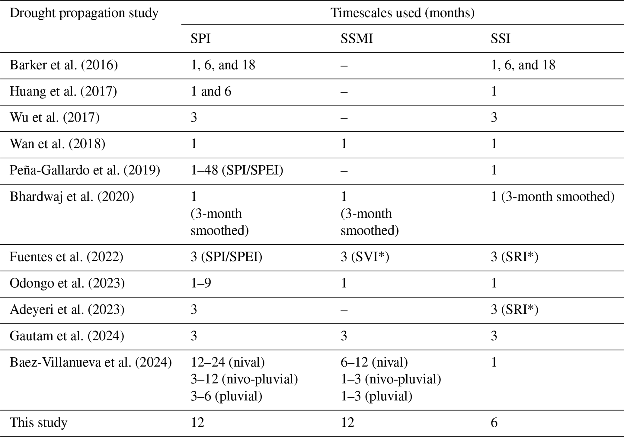
Note: SVI refers to Standardized Vegetation Index, calculated based on the MODIS NDVI index and described in Peters et al. (2002). SRI refers to the Standardized Runoff Index (Shukla and Wood, 2008).

3.5 Drought propagation analysis

Using the timescales that maximize correlations identified in Sect. 3.4, we compute the SPI, SSMI, and SSI indices to examine the transition from meteorological to hydrological droughts in the duration–intensity space, passing through soil moisture drought (SPI → SSMI → SSI; Fig. 2e). In other words, we analyze the duration (in months) and the intensity, quantified as the temporally averaged index value during its respective drought duration, with a focus on the 1998/99 and 2012–2016 (a subperiod of the Chilean megadrought) events, which simultaneously affected our case study basins. We also compare the drought propagation portrayals derived from the timescales identified here against other criteria adopted in recent studies (Table 3). These include propagation analyses using 1- (Wan et al., 2018) and 3-month (e.g., Gautam et al., 2024) timescales for SPI, SSMI, and SSI calculations and varying timescales for these indices depending on the hydrological regime of the target basin (e.g., Baez-Villanueva et al., 2024).

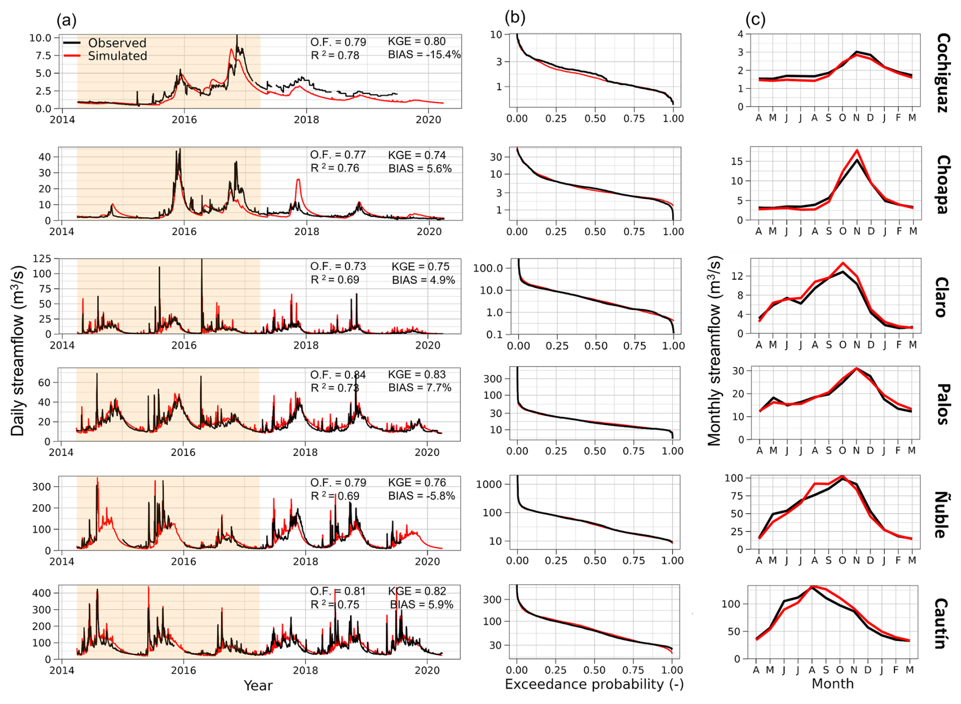
Figure 3 Comparison between simulated and observed streamflow for all basins in terms of (a) daily time series (April 2014 to March 2020), (b) daily flow duration curves (vertical logarithmic scale), and (c) mean monthly runoff. In panel (a), the shaded area represents part of the calibration (yellow) and evaluation (white) periods, and OF, R², KGE, and BIAS indicate the values for the objective function (Eq. 1), coefficient of determination, Kling–Gupta efficiency, and percent bias over the evaluation period, respectively. The results in panels (b) and (c) correspond to the evaluation periods (April 2006–March 2010 and April 2017–March 2020) combined.

4 Results

4.1 Hydrological model performance

Figure 3 displays hydrological model calibration and evaluation results for the six study basins, showing an overall good agreement between observed and simulated streamflows. The value of the objective function (Eq. 1) during the evaluation period is higher than 0.73 in all basins (Fig. 3a). The minimum KGE during the calibration period is 0.74 (Choapa), whereas the highest KGE values are 0.83 (Palos) and 0.82 (Cautín). Negative biases (i.e., underestimation of runoff volumes) are obtained for Cochiguaz (−15.4 %) and Ñuble (−5.8 %), while small (<8 %) positive biases are obtained in the remaining basins. In general, the observed daily flow duration curves are well simulated by the SUMMA model in all catchments (Fig. 3b), including its mid-segment slope (20 %–70 % flow exceedance probabilities); nevertheless, there is an overestimation of low flow volumes with exceedance probabilities larger than 90 % in the Choapa and Claro catchments (<2 m³ s⁻¹), which could be explained by the inadequate model physics representation, including, but not limited to, the lack of a common aquifer enabling water exchange among grid cells in our SUMMA configuration and/or biases in the forcing dataset that impact the accumulation and melting of snow. The streamflow seasonality is well reproduced by the SUMMA model in all basins (Fig. 3c), though there is an overestimation (<10 %) of mean monthly flows during September–November (i.e., when snowmelt occurs) at the Choapa and Claro river basins and during March–October (i.e., when rainfall events occur) at the Ñuble and Cautin river basins.

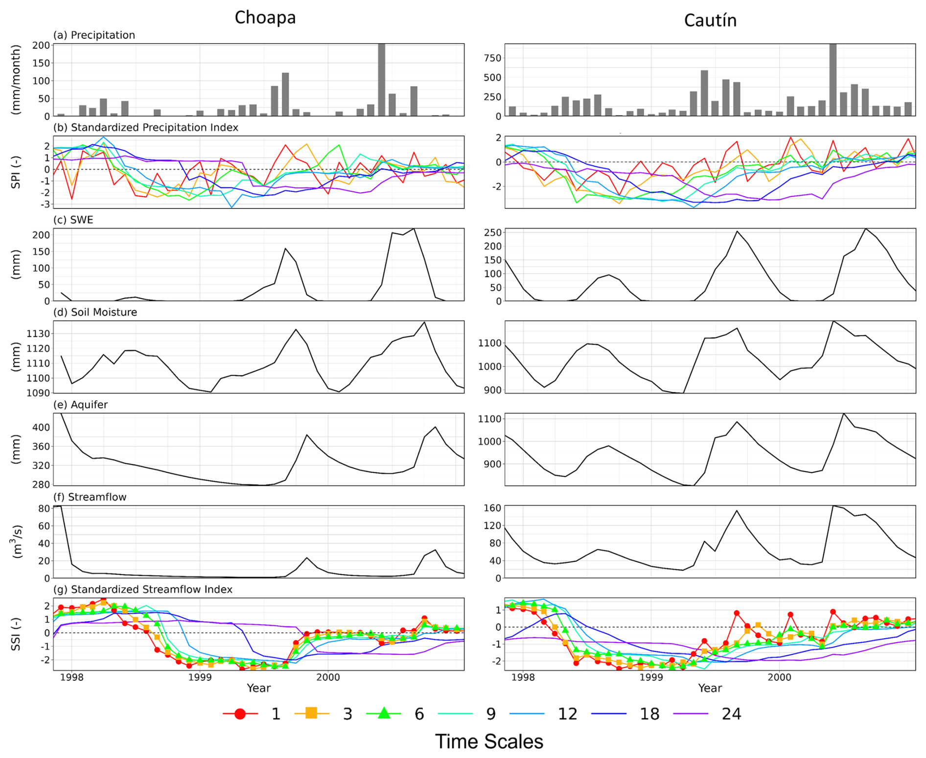
Figure 4 Monthly time series of (a) precipitation, (b) SPI-n, (c) SWE, (d) total soil moisture, (e) aquifer storage, (f) streamflow, and (g) SSI-n for the Choapa (snowmelt-driven, left) and Cautín (rainfall-driven, right) river basins. Monthly precipitation and SPI are obtained from the CR2MET meteorological product, whereas the remaining variables are obtained from SUMMA model simulations during January 1998–December 2000. SPI-n and SSI-n are displayed for timescales n=1, 3, 6, 9, 12, 18, and 24 months. Timescales of 1, 3, and 6 months for the SSI are highlighted with circles, squares, and triangles, respectively, due to their widespread use.

4.2 Effects of timescale on drought characteristics

Figure 4 illustrates the time series for different simulated hydrological variables and for the SPI and SSI indices computed at different timescales for the Choapa and Cautín river basins. We focus on a 3-year period (1998–2000) that includes the year 1998, a remarkably dry year spanning a 6-month period (July–December) with abnormally low precipitation amounts (Kreibich et al., 2022). Such a precipitation deficit had a noticeable impact on snow accumulation, especially in the Choapa River basin (snowmelt-driven), and affected other variables to a lesser degree, including soil moisture (agricultural drought) and aquifer storage, whose levels were even lower than those recorded in subsequent years. Ultimately, the meteorological drought translated into lower streamflow values over the course of 1998 and even 1999.

Figure 4b and g show the impacts of timescale selection on the SPI and the SSI, with substantial differences between 1-month indices and timescales larger than 12 months (18 and 24 months). This is especially noticeable in the SSI time series of the Choapa River basin, where a similar behavior over time is observed for SSI-1, SSI-3, SSI-6, and SSI-9, with index values smaller than −1 between October 1998 and September 1999. Nevertheless, the onset of hydrological drought is detected in May 1999 (end of 1999) if an 18-month (24-month) timescale is used to compute the SSI. Notably, Fig. 4g shows that even a 1-month timescale in SSI calculations can distort the actual variability in streamflow considerably.

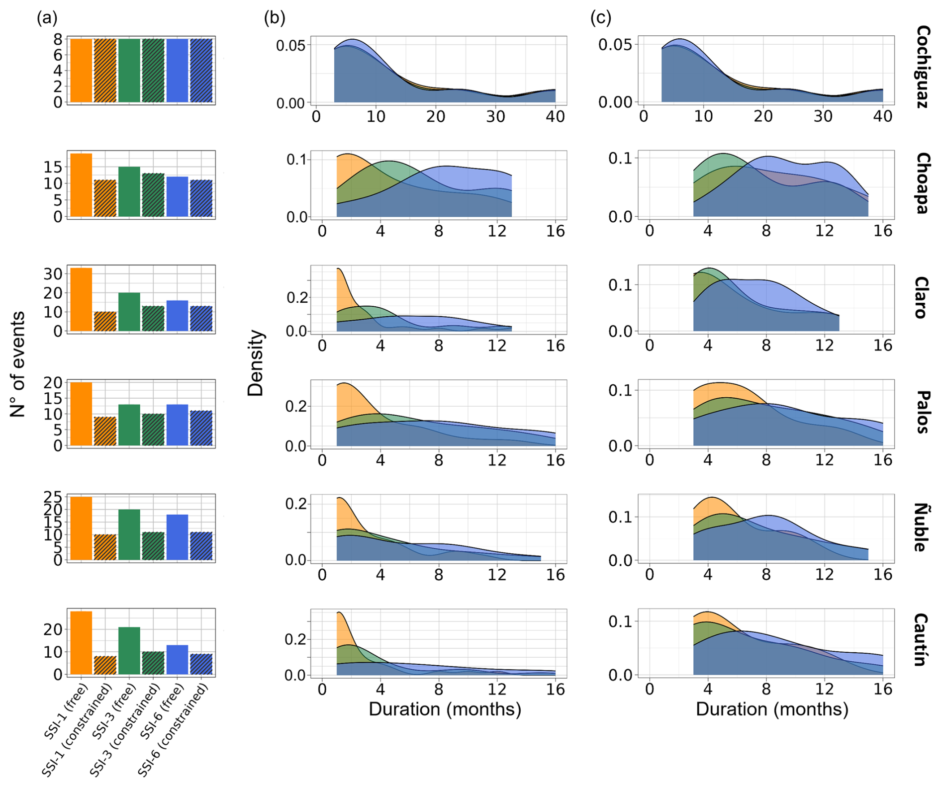
Figure 5 Effects of the choice of temporal scale (1, 3, and 6 months) in SSI calculations and duration restrictions on (a) the frequency and (b, c) the duration of hydrological droughts detected during the period 1983/84–2019/20. Probability distributions of drought durations are displayed for the cases of (b) no restrictions regarding the duration of droughts (i.e., it is possible to detect 1-month, “free”, events) and (c) a minimum drought duration of 3 months (i.e., “constrained”) for event detection; i.e., SSI-$n<-\mathrm{1}$ during at least 3 consecutive months.

The choice of timescales used to compute the SSI can also affect the estimated frequency and duration of hydrological drought events. This is illustrated in Fig. 5, which compares the number of hydrological droughts detected with SSI-1, SSI-3, and SSI-6 and the probabilistic distribution of their duration over the entire simulation period (April 1983–March 2020). Figure 5a shows substantial differences in the number of events depending on the criteria and timescale used, with the only exception being the Cochiguaz River basin. In general, the number of events detected with the free criterion decreases for longer timescales, as opposed to the constrained criterion, for which such numbers tend to remain constant or even increase (see, for example, the Choapa River basin). The largest discrepancies are found in the rainfall-dominated catchments; for example, in the Cautín River basin, 28 and 13 events were detected with SSI-1 and SSI-6, respectively, using the free criterion. Figure 5b and c display the empirical probability density functions of drought durations obtained with the free and constrained criteria, for all basins and timescales, and Table 4 includes the average durations considering all the events during the analysis period. As for the frequency, we found no changes in the Cochiguaz River basin; however, the choice of timescale has considerable effects on drought durations in rainfall-driven catchments, especially with the free criterion, with a transition from positively skewed probability density functions with averages between 1–3 months when using SSI-1 to more homogeneous distributions, centered around 8 months, when using SSI-6.

Table 4 Mean duration (in months) of drought events for each case and temporal scale of SSI.

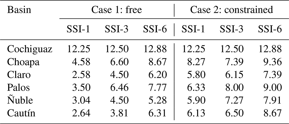
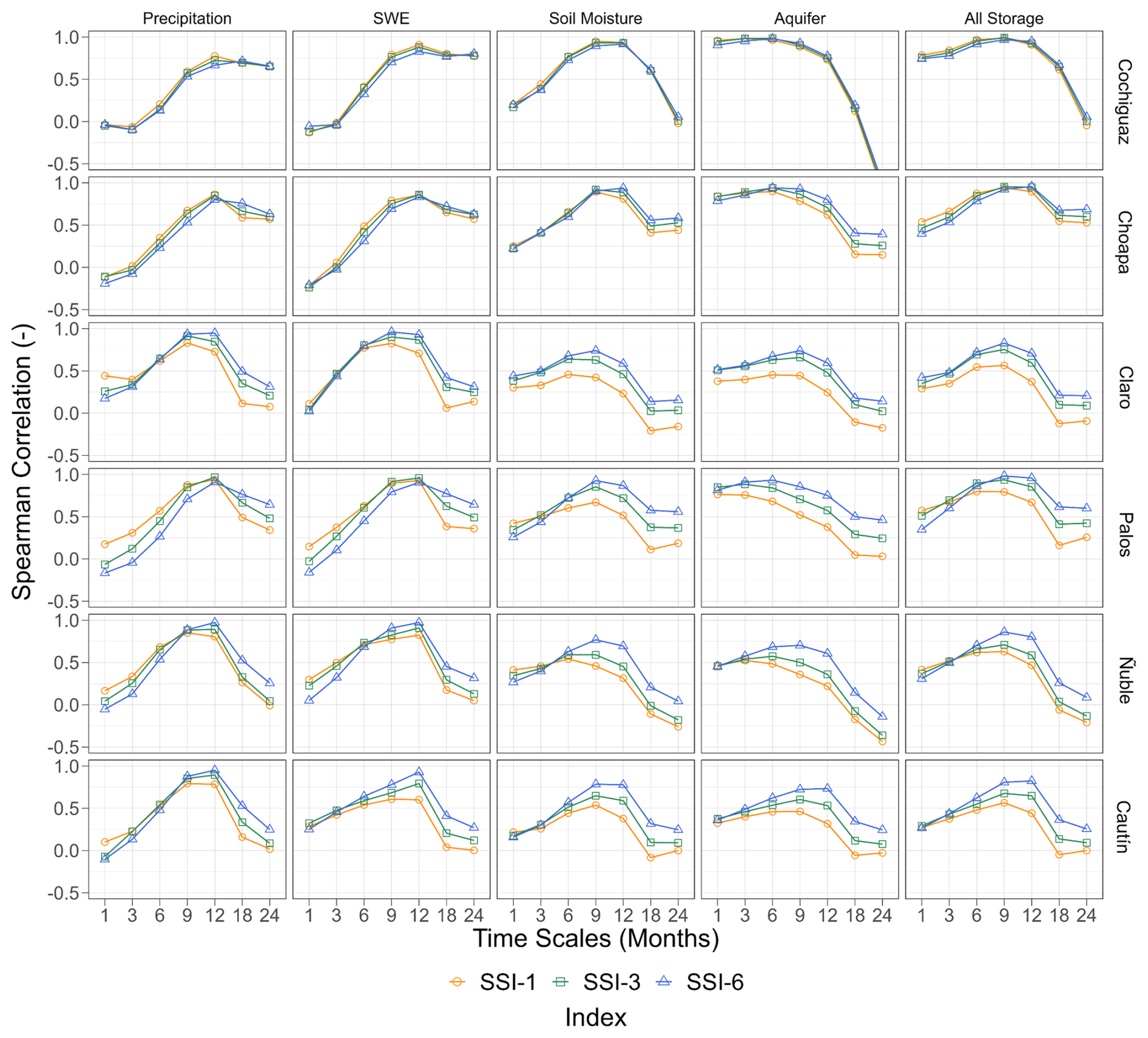
Figure 6 Spearman rank correlation coefficients between the SSI computed at different timescales (1, 3, and 6 months) and temporally aggregated (i.e., averaged) hydrological variables (columns) over the period January 1998–December 2000. The results for each case study basin are displayed in different rows.

4.3 Correlation between the SSI and hydrological variables

Figure 6 illustrates how the choice of timescale used for the SSI affects the Spearman rank correlation between this index and the main hydrological variables (precipitation and catchment storages). One can note that the differences are minimal between SSI-1, SSI-3, and SSI-6 for the two snowmelt-driven basins (i.e., Cochiguaz and Choapa). Furthermore, the shape of the curves is similar in most cases, achieving the highest correlations with precipitation and SWE on a 12-month scale and the highest correlations with soil moisture and total storage using timescales between 6 and 12 months. Notably, the strength of the relationship between the SSI and aquifer storage varies depending on the hydrological regime: in snowmelt-driven basins, the correlations are higher for timescales of 3–6 months of aquifer storage, whereas correlation is maximized with 9–12-month timescales in rainfall-dominated catchments.

In most cases, the highest (lowest) correlations are obtained using SSI-6 (SSI-1), although there are some exceptions for timescales shorter than 9 months at the Palos and Ñuble river basins (mixed regime), where higher correlations are achieved when using SSI-1. The impacts of the timescale on correlation results are considerably larger in basins with mixed or rainfall-dominated regimes, where there is larger dispersion in the correlation achieved by the indices, reaching differences up to 0.5 in the Ñuble and Cautín river basins for a 12-month scale. Similarly, a progressive increase in the dispersion of correlations is observed when evaluating indices at larger timescales (>9 months) for all storages in mixed and rainfall-driven catchments. Overall, the results in Fig. 6 suggest that, if the aim is to investigate the relationship between the main hydrological variables and fluctuations in the SSI, the choice of the timescale used to compute this index becomes less relevant in snowmelt-driven basins with large baseflow contributions, compared to rainfall-dominated catchments.

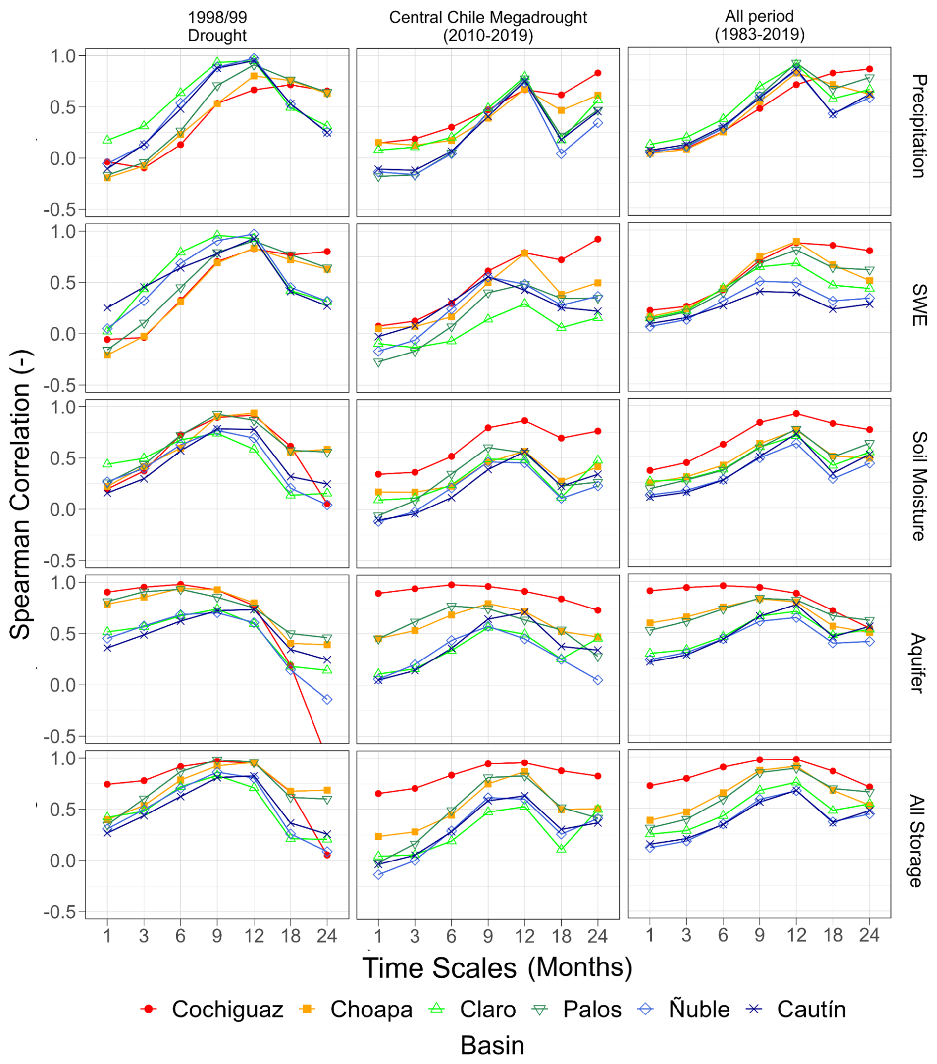
Figure 7 Spearman rank correlation coefficients between SSI-6 and temporally aggregated/averaged catchment-scale hydrological variables (rows) for three different periods: (a) the October 1998–September 1999 drought event, (b) the central Chile megadrought (April 2010–March 2019), and (c) the entire analysis period (April 1983–March 2020).

Figure 7 explores the potential effects of hydrological regimes on the Spearman rank correlations between SSI-6 and the hydrological variables aggregated at different timescales for three periods: the 1998/1999 drought event, the central Chile megadrought (2010–2019), and April 1983–March 2020 (the results for SSI-1 and SSI-3 are presented in Figs. S1 and S2 in the Supplement). The examination of different storages over the entire period (April 1983–March 2020) reveals that, in general, higher Spearman rank correlations are obtained in arid and snowmelt-driven basins compared to humid and rainfall-driven basins, regardless of the timescale analyzed. In other words, there are stronger relationships with SSI-6 in the northern regions (aridity index >2 and mean annual P<400 mm yr⁻¹), which gradually become weaker towards the south (aridity index <0.5 and mean annual P>2000 mm yr⁻¹), following central Chile's hydroclimatic gradient. Such patterns are more evident when all catchment storages are aggregated (last row in Fig. 7) and to a smaller degree in individual storages (SWE, soil moisture, and aquifer storage). Such relationships between the strength of the correlations and the hydroclimatic regime are also obtained for SSI-3 (Fig. S2) and, to a greater extent, for SSI-1 (Fig. S1).

Figure 7 also shows that the magnitude of correlations between hydrological variables and SSI-6 varies with the analysis period, especially during exceptionally dry and short periods. For example, the relationships between SSI-6 and precipitation in rainfall-dominated and mixed-regime catchments (Claro, Palos, Ñuble, and Cautín) are stronger during the 1998/99 drought, with Spearman rank correlations near 1 for a 9-month scale, whereas the remaining periods yield correlations that do not exceed 0.7 at the same temporal scale. Considerable differences are also obtained for SWE, with high correlations (>0.7) in all basins for the 9- and 12-month timescales during the 1998/99 event and lower correlations during the central Chile megadrought. The selection of the analysis period also yields differences in the correlation with soil moisture and aquifer storage. Notably, higher correlations with ≤9-month aquifer storage are obtained during the 1998/99 event in Choapa and Palos, where the snowmelt contribution to runoff is substantial.

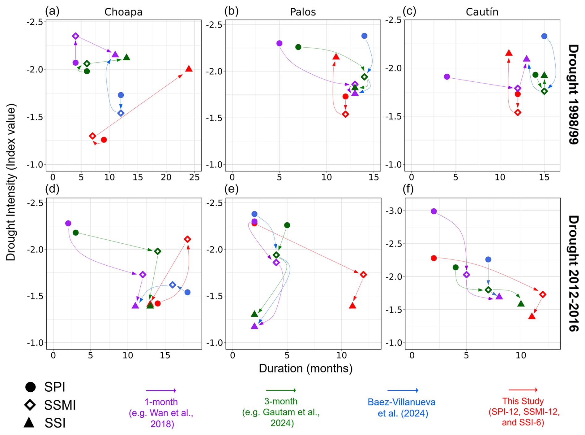
Figure 8 Propagation from meteorological (circles) to soil moisture (diamonds) and hydrological (triangles) droughts for two selected drought events (1998/99 and 2012–2016, displayed in different rows) and three basins with different hydrological regimes: (a, d) Choapa (snowmelt-driven, left), (b, e) Palos (mixed regime, center), and (c, f) Cautín (rainfall-driven, right). The x axis shows the duration in months, and the y axis displays the intensity. The colors indicate trajectories obtained with the temporal scales recommended by different studies.

4.4 Effects of temporal scale on drought propagation

To what extent can the choice of temporal scale affect the portrayal of drought propagation across different hydrological regimes? Figure 8 displays the transition of meteorological towards soil moisture and hydrological droughts in the duration–intensity space for the Choapa (snowmelt driven), Palos (mixed regime), and Cautín (rainfall driven) river basins (results for the remaining basins are included in Fig. S3 in the Supplement). The results show that different timescales affect drought duration and intensity and the progression of such characteristics in a specific hydrological system. For example, the results for the 1998/99 event in the Choapa River basin show that using 1-month (purple; Wan et al., 2018) and 3-month (green; Gautam et al., 2024) timescales and the timescales derived here yield a transition toward a relatively longer and more intense hydrological drought, compared to the meteorological drought, whereas the timescales recommended by Baez-Villanueva et al. (2024; blue) provide a progression toward a more intense and slightly shorter hydrological drought. In the Palos River basin, we find that, for the same event and the timescales derived from this study (red), the soil column buffers the intensity of the meteorological drought, which transitions toward a shorter and more intense hydrological drought during the 1998/99 event. Using 1-month and 3-month timescales for SPI, SSMI, and SSI yields a transition from a very intense and short meteorological drought towards a longer and smoother hydrological drought; nevertheless, the timescales recommended by Baez-Villanueva et al. (2024; blue) yield a decline in intensity and a slightly shorter duration from meteorological to hydrological drought. In the Cautín River basin, all propagation trajectories obtained for the same event are very different. Other discrepancies in drought trajectories are obtained in all combinations of basin/event (Figs. 8 and S3).

Note that the relative location of soil moisture drought within the trajectories can be very different depending on the timescale selected. An interesting example is the 2012–2016 event at the Choapa River basin, for which the four trajectories differ considerably; in particular, the timescales found here yield very similar durations for meteorological and hydrological droughts and a more intense and prolonged soil moisture drought. For the same event, 1-month (purple) and 3-month (green) scales and the temporal scales from Baez-Villanueva et al. (2024) yield trajectories with decreasing intensity and longer durations moving from meteorological to soil moisture and hydrological droughts in the Cautín River basin; however, the timescales derived from our analyses (red) indicate a longer soil moisture drought in comparison with the resulting hydrological drought. Notably, Fig. 8 also shows that our trajectories (red symbols and arrows) for the two events analyzed are similar at the Palos and Cautín river basins, suggesting a similar propagation pattern between mixed and rainfall-driven regimes. The same pattern is also obtained for the Ñuble River basin (Fig. S3 in the Supplement).

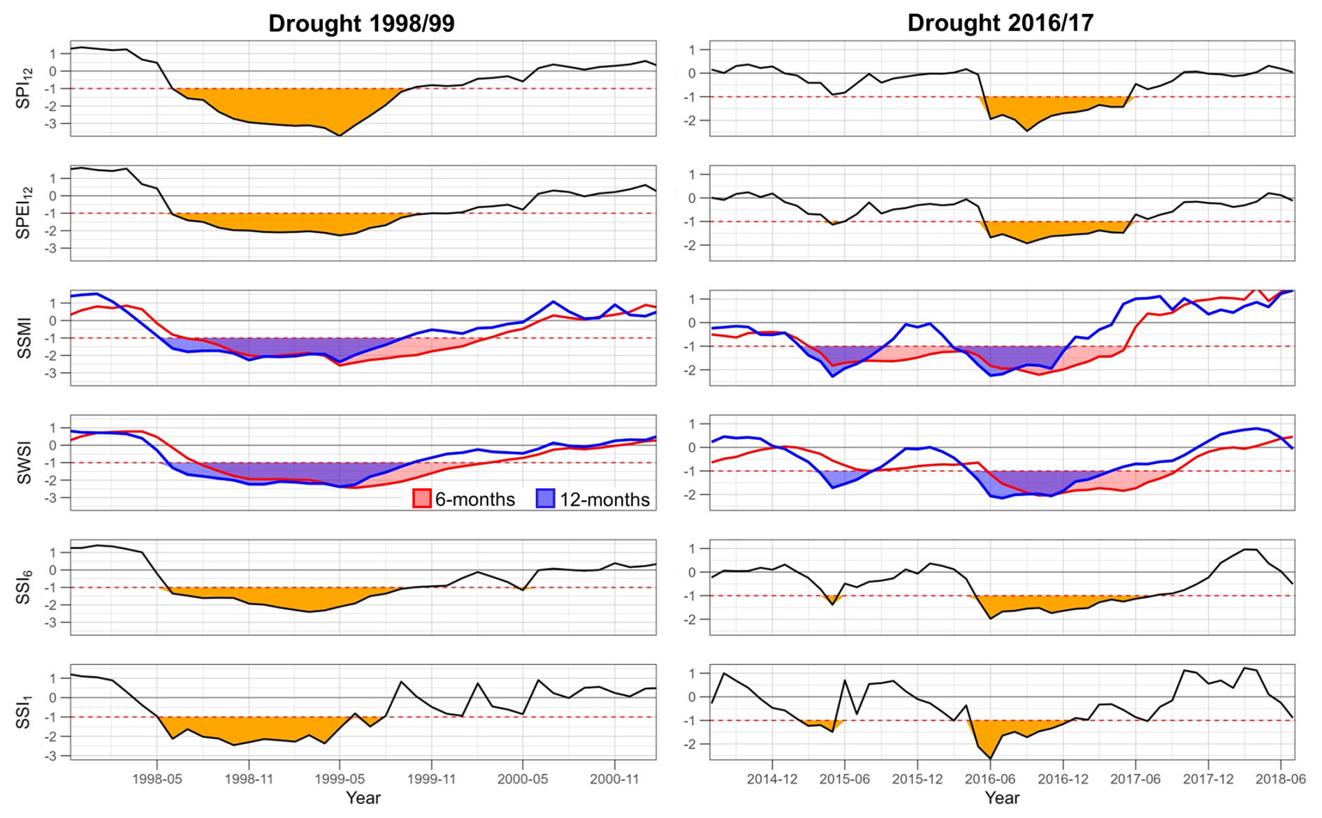
Figure 9 Monthly time series of standardized indices at the Cautín River basin, computed with the timescales selected from the correlation analyses. The orange areas illustrate the onset, end, and duration of the 1998/99 drought (left) and the 2016/17 drought (right), according to the different indices. For the SSMI and the SWSI, two timescales (6-month and 12-month values) are displayed for comparison.

It should be noted that the timescales selected based on maximum correlation with SSI-6 (or any other timescale) do not necessarily yield similarities between the onset, duration, and end obtained with different indices for an individual event. Figure 9 illustrates this point for two events at the Cautin River basin. The results show that SSMI-12 and SWSI-12 correlate well with the temporal evolution of SSI-6 for the 1998/99 drought; nevertheless, the temporal variability in SSMI-12 during the 2016/17 event shows a closer agreement with SSI-1 compared to SSI-6, which, in turn, does not match with SSMI and SWSI at any timescale but yields a similar onset, duration, and end detected with SPI-12 and SPEI-12. Even more, the SSMI and SWSI reflect soil moisture and total storage deficits, respectively, before the precipitation deficits detected with SPI-12 using a −1 threshold.

5 Discussion

5.1 Drought detection and characteristics

This study reveals additional insights for hydrological drought analysis based on SSI estimates. Despite the results confirming well-known effects of the temporal scale selected for aggregating streamflow on the frequency and duration of hydrological droughts detected with the SSI (e.g., Barker et al., 2016; Teutschbein et al., 2022), such impacts are minor in slow-reacting catchments (e.g., Cochiguaz River basin, with average drought durations ranging from 12.3–12.9 months), which can be explained by the buffering effect of snowpack and by soil moisture and aquifer storage. Conversely, the impacts of the temporal-scale and duration constraints are more noticeable in rainfall-driven basins, where considerable rainfall contributions to runoff occur during winter. Note that the relatively longer average drought durations found in semi-arid, snowmelt-driven catchments (which also hold the largest baseflow contributions) align well with previous studies linking drought duration with catchment storage properties (Van Loon and Laaha, 2015; Barker et al., 2016).

Although the model's overestimation of low flow volumes in Choapa and Claro (Fig. 3) affects the accuracy (i.e., closeness to reality) of the number and duration of detected events (Fig. 5), this artifact does not alter our conclusions, as all analyses focus on the impact of methodological choices related to index calculations using simulated variables, regardless of the fidelity of model representations. Even more, all the correlation and drought propagation analyses were performed in the model's world; therefore, streamflow biases should not impact the extent to which variables or drought indices computed with different timescales relate to each other.

5.2 Interpretability of the SSI across hydrological regimes

In rainfall-driven basins, we found a strong connection between SSI-6 and precipitation deficits (i.e., a strong link between hydrological and meteorological drought), whereas soil and aquifer storages become more important in basins with increased aridity, in agreement with previous studies (e.g., Haslinger et al., 2014). Specifically, in semi-arid basins, the SSI reflects the variability in >12-month aggregated precipitation and SWE, as well as fluctuations in aquifer storage at <9-month timescales. Our results also show that dependencies between correlations and hydroclimatic regimes change with the analysis period (Fig. 7), highlighting the uniqueness of each drought event.

We show that aggregating streamflow into seasonal periods (i.e., 3 and 6 months) for SSI calculations does not necessarily attenuate potential relationships with other variables of the water cycle (e.g., see results for the Cochiguaz River basin, Fig. 4). Even more, shifting from SSI-1 to SSI-3 and SSI-6 yields a stronger influence of soil moisture and aquifer storage for nearly all temporal scales in mixed- and rainfall-driven-regime basins. On the other hand, shifting from SSI-6 to SSI-3 and SSI-1 exacerbates the connections found between the strength of the correlations and the hydroclimatic regime of the basin analyzed. These results suggest that the timescale used for the SSI should be selected based on the specific purposes and the hydroclimatic regime if the aim is to enhance the interpretability of physical mechanisms.

Although previous studies have shown that meteorological droughts may propagate differently depending on hydroclimatic characteristics and system properties (e.g., Van Loon et al., 2014; Van Loon and Laaha, 2015; Barker et al., 2016; Apurv et al., 2017), we show that such portrayal may be very sensitive – for a given combination of event and catchment – to the subjective choice of the timescale used to compute standardized indices (Fig. 8). Furthermore, the results presented here reveal pitfalls in drought propagation analyses when selecting timescales for standardized indices based on correlation analyses and fixed thresholds. Specifically, the results in Fig. 9 for the 2016/17 event suggest that, given a drought event affecting a unique hydrological system, the thresholds for standardized meteorological and soil moisture indices that enable interpreting causality in time (including onset, duration, and end) may differ, and variable threshold approaches (e.g., Van Loon and Laaha, 2015; Odongo et al., 2023) may be more appropriate to this end.

Our results also show that, given a well-defined criterion to compute standardized indices (in this study, SPI-12, SSMI-12, and SSI-6), the trajectories of the same drought event may differ considerably among catchments. Likewise, propagation trajectories can differ substantially among drought events within a particular catchment (Fig. S4 in the Supplement). Overall, this work suggests that any results derived from standardized indices should be interpreted cautiously, checking carefully the reasoning behind the selection of the selected drought indices and their temporal scales.

5.3 Implications for operational practice

In Chile, the current legislation states that hydrological droughts between the Atacama and Araucanía regions, a large area that encloses the six basins examined here, are officially declared based on SSI-6 – regardless of the hydroclimatic regime – or the SPI (DGA, 2022). Even more, DGA (2022) considered spatial differences in that area regarding the SPI, using a 12-month timescale between the Atacama and Maule regions (which enclose our snowmelt-driven and mixed regime basins) and a 6-month timescale between the Ñuble and Araucania regions (which enclose the two rainfall-driven basins analyzed here).

In other international agencies, it is common practice to use multiple indicators for drought monitoring and early warning systems (e.g. Bachmair et al., 2015), rather than relying only on standardized indices such as the SPI and SSI. These indicators often include satellite products and variables simulated by hydrological models, which aligns with the recommendations outlined in the WMO's Handbook of Drought Indicators and Indices (Svoboda and Fuchs, 2016). In particular, the European Drought Observatory (EDO) uses the Combined Drought Index (CDI; Sepulcre-Canto et al., 2012), which simultaneously considers three types of indicators: the SPI, the anomalies of simulated soil moisture in the LISFLOOD hydrological model (van der Knijff et al., 2010), and anomalies of the Fraction of Absorbed Photosynthetically Active Radiation (FAPAR; Gobron et al., 2010). The former is derived from the MOD15A2H satellite product and is related to vegetation growth and crop productivity. Similarly, the United States Drought Monitor (USDM; Svoboda et al., 2002) combines the Palmer Drought Severity Index (PDSI; Palmer, 1965), the SPI, and soil moisture and streamflow percentile-based indicators in their evaluations.

The results presented here suggest that the choice of timescales for the SSI should be made depending on the hydroclimatic features of the basin of interest and the target application(s). In this regard, we find that the temporal scale selected for the SSI is less relevant in snowmelt-driven basins than in mixed regimes and rainfall-dominated catchments. For real-time hydrological drought monitoring or to characterize short and intense events, 1–6-month timescales may be convenient, whereas ≥12 months would be more suitable for multi-year drought detection, since long timescales help to smooth the original temporal variability and capture the long-term effects of precipitation deficits (Fig. 4). If surface water is used for irrigation, the choice of timescale should also consider the specific crop characteristics and, in particular, the capability (i.e., period length) to survive under water scarcity conditions.

5.4 Limitations and future work

In this study, we did not consider in situ or remotely sensed observations of SWE, soil moisture, and aquifer storage in the calibration process, relying on the capability of the SUMMA model to replicate streamflow signatures. We did not explore the effects of using alternative model parameterizations (e.g., stomatal resistance, lateral fluxes) or spatial configurations (e.g., spatially varying soil layer depths) on the results and conclusions obtained. Moreover, we did not explore variable threshold methods (e.g., Van Loon and Laaha, 2015; Odongo et al., 2023) for drought detection and propagation analyses.

Future work could expand the analyses presented in this study by exploring tradeoffs between the timescales used to compute the SSI and the choice of statistical distributions (e.g., Svensson et al., 2017; Teutschbein et al., 2022), the parameter estimation method (e.g., Tijdeman et al., 2020), the choice of reference period (set here as April 1983–March 2013), or the threshold selection criteria (e.g., Wanders et al., 2015; Odongo et al., 2023). Finally, the analyses presented here could be expanded to a larger number of basins that consider a greater diversity of features (e.g., Vásquez et al., 2021; Muñoz-Castro et al., 2023) in order to examine whether the timescales of hydrological variables (e.g., precipitation, soil moisture, SWE) that maximize the correlation (or “optimal” timescales) with the SSI are related to physiographic attributes such as contributing area, slope, elevation, geology, land cover, and soil type, among others. A simple stratification of attribute values by optimal timescale, or any other hydrological descriptor of interest (e.g., Sawicz et al., 2011; Almagro et al., 2024), could provide valuable insights, complementing previous drought investigations using large samples of catchments. For example, Van Loon and Laaha (2015) found that geology and land use were relevant controls for hydrological drought duration. Peña-Gallardo et al. (2019) concluded that elevation and vegetation coverage are the main factors controlling the diverse response of SSI to SPEI timescales. More recently, Brunner and Stahl (2023) confirmed that land surface processes are required to explain the temporal clustering of hydrological droughts. More generally, additional large-sample hydrology analyses could help to improve our understanding of the main drivers affecting drought occurrence and propagation across different hydroclimates.

6 Conclusions

The Standardized Streamflow Index (SSI) has been widely used for hydrological drought monitoring, forecasting, and propagation analyses. Nevertheless, there is limited understanding of how the subjective choice of timescales affects the characterization of these events and, more importantly, which hydrological variables are related to SSI fluctuations. In this study, we intend to fill these gaps by applying the SUMMA hydrological model coupled with the mizuRoute routing model in six hydroclimatically different basins located on the western slopes of the extratropical Andes. We also illustrate how sensitive the portrayal of drought propagation is to the timescales used to compute popular standardized indices such as the SPI and the SSMI. Our main findings are as follows:

1. The timescale used to compute the SSI and the minimum duration to define hydrological drought occurrence can largely affect the estimated duration and frequency of these events, especially in rainfall-driven catchments.

2. The strength of the relationship between the SSI and hydrological storages/fluxes is less affected by the choice of timescale of the SSI in snow-driven regimes compared to mixed and rainfall-dominated basins, where the dispersion of correlations progressively increases when using explanatory variables temporally aggregated for more than 9 months.

3. Higher correlations are achieved when SSI-6 is contrasted against hydrological variables aggregated at 9 and 12 months, except for aquifer storage at the Cochiguaz basin (snowmelt-driven), and lower correlations are obtained for timescales longer than 12 months. When SSI-1 and SSI-3 are used, the correlations are maximized at shorter temporal scales (compared to SSI-6) for some combinations of hydrological variables and basins (e.g., aquifer storage at Palos and Ñuble).

4. When analyzing the entire period (April 1983–March 2020), higher correlations between SSI-6 and hydrological variables are achieved for snowmelt-driven basins, and these progressively decrease towards rainfall-driven regimes. This pattern becomes stronger when the total water storage within a basin is considered. Nevertheless, such a pattern becomes less clear and dependent on the temporal scale of explanatory variables during drought periods.

5. The portrayal of drought propagation may change drastically depending on the choice of timescales used to compute standardized indices. In this regard, different criteria may reveal opposite trajectories of drought propagation for the same event in a basin.