Effect of the spatial resolution of digital terrain data obtained by drone on urban fluvial flood modeling of mountainous regions

Analysis of the effect of the resolution and quality of terrain data, as the most sensitive input to 2D hydrodynamic modeling, has been one of the main research areas in flood modeling. However, previous studies have lacked discussion on (1) the limitations of the target area and the data source and (2) the underlying causes of simulation bias due to different resolutions. This study first discusses the performance of a high-resolution digital terrain model (DTM), acquired using a drone, for flood modeling in a mountainous riverine city; analyses the effect of the DTM resolution on the results using grid resolutions from 6 cm to 30 m; and then investigates the root causes of the effect based on topographic attributes. Xuanhan, a riverine city in the mountainous region of Southwestern China, was used as the study area. The Hydrologic Engineering Center's River Analysis System (HEC-RAS) 2D model was used for all simulations, and the results generated using a 6 cm DTM acquired by drone were used as a benchmark. The results indicate that flood characteristic simulations exhibit noticeable stepwise changes as the DTM resolution varies. DTMs with a resolution better than 10 m are more effective with respect to capturing the terrain's undulating features in the study area, which is crucial for accurately modeling the inundation area. However, to accurately capture topographic features related to elevation differences, the resolution should preferably be better than 5 m, as this directly affects the accuracy of flood depth simulation. The analysis of topographic attributes provides theoretical support for determining the optimal resolution to meet simulation requirements.

1 Introduction

Over the past decade, floods, storms, and droughts have caused 80 %–90 % of the global natural disasters, with floods alone accounting for over 40 % (WHO, 2020). More than 2 billion people worldwide have been impacted by flood events, with flood-related fatalities comprising half of the total deaths from natural disasters (Alderman et al., 2012; Samela et al., 2016). With the continuous development of residential areas on floodplains and the increasing frequency of extreme precipitation events caused by the El Niño phenomenon, nearly 40 % of the global cities will be located in flood-prone areas by 2030, especially mountainous cities along rivers (Güneralp et al., 2015; Corringham and Cayan, 2019; Muthusamy et al., 2021).

Taking the mountainous area of Southwestern China as an example, the expansion of numerous towns along major rivers in recent decades has been influenced by complex topography and steep terrain. Different from the urban waterlogging caused by the impermeable surfaces and drainage networks in the plain cities, mountainous cities along rivers face distinct challenges. On the one hand, the steep terrain accelerates the process of runoff entering rivers during heavy-rainfall events; on the other hand, early urban development in these areas was constrained by limited financial resources and inadequate planning foresight, resulting in substandard river flood control infrastructure and poorly planned residential zones. Consequently, these areas are more susceptible to inundation caused by the rapid rise and fall of river floods. With the growing impacts of climate change and extreme weather events, flood inundation in these regions is expected to cause far greater damage than previously anticipated (Xing et al., 2018; Utlu and Ozdemir, 2020). Therefore, identifying potential flood-prone areas in mountainous cities along rivers is critical for flood risk assessment and future urban planning. Hydrodynamic flood modeling methods are indispensable for flood inundation simulation and risk management, and various GIS-based hydrodynamic flood models have been developed in recent years (Azizian and Brocca, 2020; Utlu and Ozdemir, 2020).

Utilizing hydrodynamic models for flood risk assessment and management necessitates a variety of data inputs, including topographic and hydrological information. Over the past decade, advancements in satellite remote-sensing technology and computational capacity have facilitated the broader application of 2D hydrodynamic models to flood simulations (Bates, 2012; Yan et al., 2015; Utlu and Ozdemir, 2020). The most sensitive input affecting the 2D flood inundation simulation attributes (depth, extent, and velocity) is the digital elevation model (DEM); thus, this places higher requirements on the quality and resolution of DEMs (Cook and Merwade, 2009; da Costa et al., 2019). Currently, freely available global DEM datasets are primarily sourced from satellite imagery and include options such as the SRTM DEM (30–90 m), ASTER global DEM (ASTER GDEM; 30 m), MERIT DEM (90 m), and ALOS DEM (12.5–30 m). Although coarse-resolution DEMs (> 30 m) are suitable for simulating large-scale flood events in large basins, they are less effective with respect to capturing the detailed topographic features of mountainous terrain or complex urban settings (Saksena and Merwade, 2015; Ogania et al., 2019; Utlu and Ozdemir, 2020). Developed countries have leveraged satellite-based and airborne technologies, such as lidar or synthetic aperture radar (SAR), to generate digital terrain models (DTMs) and digital surface models (DSMs) with enhanced topographic detail, achieving resolution accuracy down to the centimeter scale (Md Ali et al., 2015).

In recent years, rapid advancements in drone technology have significantly improved the capabilities of civilian small-scale drones. Equipped with features such as flight path planning, automatic flight control, and mountable sensors, these drones have overcome many limitations of traditional surveying equipment, including poor portability, high operational complexity, and cost. Civilian drones are now widely utilized across fields such as hydrology, agriculture, and forestry (Castaldi et al., 2017; Loladze et al., 2019; Acharya et al., 2021). Drones enable the acquisition of high-resolution digital terrain information without being constrained by time or geographic location, and they can be deployed on demand, providing reliable terrain data for precise 2D hydrodynamic model simulations of flood inundation (Meesuk et al., 2015; Cook, 2017). Currently, there are two mainstream methods for obtaining high-precision DEMs using drones. One approach is to use photogrammetry techniques to derive the DEM from drone-acquired imagery. This method has relatively lower equipment and processing costs, making it more widely applicable; however, its accuracy is limited in areas with dense vegetation and often requires the establishment of ground control points. The other approach involves using drones equipped with lidar to obtain DEMs. This method has the advantage of penetrating vegetation and can acquire high-precision terrain data under all weather conditions, but it comes with higher equipment and processing costs (Muthusamy et al., 2021; Acharya et al., 2021; Naranjo et al., 2021). In theory, as long as the model can process high-resolution DEMs, higher-resolution data will yield more accurate simulation results (Muthusamy et al., 2021). However, when obtaining and processing high-resolution DEMs over large areas, practical challenges arise due to drone endurance limitations and the increased computational burden. These challenges grow as the required resolution for flood simulations increases, posing difficulties for researchers and professionals who are not experts in the surveying field (Abily et al., 2016). Therefore, rather than pursuing the highest possible resolution, achieving an optimal balance between simulation accuracy and efficiency is critical for meeting models' requirements (Xing et al., 2018).

Since the introduction of remote-sensing imagery into hydraulic modeling, the impact of the digital terrain data resolution on flood simulations has become a key area of research. Saksena and Merwade (2015) employed a resampling technique and a hydraulic model to analyze the relationship between a series of DEM resolutions from 3 to 100 m and the extent of flood inundation in different rivers. Their findings demonstrated a positive linear correlation between the DEM resolution, water surface elevation, and inundation extent, with coarser resolutions resulting in larger inundation areas, often leading to overprediction. However, the applicability of this conclusion is limited to specific rivers and watershed characteristics. Some researchers have found that, when it comes to surface flooding (such as roads and towns along rivers), the relationship between the DEM resolution and flood characteristic simulation results (such as range and depth) is not strictly linear. Moreover, studies have shown that, even when the DEM resolution is held constant, simulation results can vary significantly depending on the source of the terrain data. Saksena and Merwade (2015) found that flood simulation results using a 30 m DEM resampled from a lidar DEM were more accurate than those derived from publicly available 30 m DEMs based on satellite imagery. These studies all underscore the need to account for the characteristics of the target area and data source when assessing the effect of the terrain data resolution on flood simulations to enhance the applicability of conclusions (Shen and Tan, 2020).

Most previous studies have predominantly focused on comparing errors in flood simulation characteristics (inundation area and depth), with limited exploration of the underlying causes of these errors when using data with different resolutions (Muthusamy et al., 2021). Research has mainly revolved around spatial and statistical comparisons between simulation results based on terrain data with different resolutions and benchmark conditions, which are typically derived from high-resolution satellite historical flood inundation maps, simulation results using high-precision terrain resolutions, or field investigation outcomes (Ozdemir et al., 2013; Yalcin, 2020). For fluvial flood modeling of mountainous cities, the variance in river floodplains, riverfront roadways, city streets, and structures with the undulation of the mountains should be the primary elements affecting water flow. Given the cost and challenges involved with acquiring high-resolution terrain data, more extensive research has typically concentrated on developed plains or coastal cities (Henonin et al., 2015; Xing et al., 2018; Leitao and de Sousa, 2018). These studies have generally concluded that the drainage network density, building size, and the spatial gaps between structures in DEMs of varying resolution impact flood simulations. However, such conclusions are difficult to generalize to mountainous riverside cities, where terrain undulation and rapid fluctuations in river levels exert a more significant influence on flood process.

The objectives of this study are to (a) discuss the application of high-resolution DTMs obtained by drones for fluvial flood modeling in a mountainous city, (b) use resampling techniques to examine the effect of DTMs obtained by drones at different resolutions on fluvial flood inundation simulation in a mountainous city, and (c) analyze the representation of terrain features by DTMs at different resolutions based on topographic attributes and investigate the fundamental causes of the effect. Ultimately, this study aims to establish the appropriate DTM resolution needed for fluvial flood modeling of mountainous cities.

2 Materials and methods

2.1 Study area

The study area, Xuanhan, is a city in a mountainous area of Southwestern China, located in the southern foothills of the Daba Mountains. The built-up area of the main city is 23 km², with a population of approximately 153 000 people. The city is located at the head of the Zhou River, a primary tributary of the Qujiang River basin, where the Qian River, Zhong River, and Hou River converge. At the confluence, a large reservoir was completed and became operational in 1992, with a regulation capacity of 102×10⁶ m³ (Fig. 1). The city has an average annual rainfall of 1248 mm, with over 80 % of the total precipitation occurring during the rainy season, primarily between July and September, influenced by the storm-prone Daba Mountains region. Between 1949 and 2021, the city of Xuanhan experienced 14 major floods (peak flow of 6000–10 000 m³ s⁻¹), with particularly severe floods occurring in 1982, 2004, 2005, and 2010 (peak flow exceeding 10000 m³ s⁻¹). Flooding caused by rainfall in the upper reaches of the Qian, Zhong, and Hou rivers, along with discharge from the Jiangkou Reservoir, has resulted in direct economic losses exceeding RMB 2 billion (approximately USD 279 million).

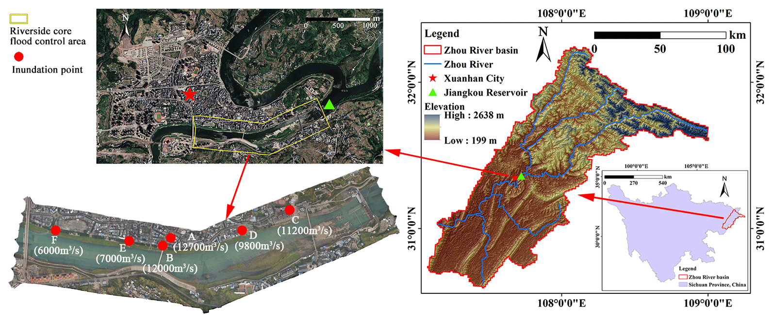
Figure 1 The location of the study area in the city of Xuanhan, China, and the flood core control area (yellow boundary line) are shown on the satellite map (© Google Earth) and in the orthophoto, including the drone survey area, flood modeling area, and six inundation points.

As can be seen from the satellite map in Fig. 1, the study area is surrounded by water on three sides. The urban development axis aligns with the river's direction, where buildings are constructed adjacent to the wide river channel and along the slopes, exhibiting marked elevation variations across the terrain. Due to land use constraints, there is no clear buffer zone between the river and the urban area, making it a typical mountainous riverside city. In accordance with the “2022 Flood Control Plan of Xuanhan” (People’s Government of Xuanhan County, 2022), this study delineates a drone survey and flood inundation simulation area that extends along the river and onto the left and right banks. This area covers six warning points that correspond to the discharge flows from the Jiangkou Reservoir and the city's inundation points, as detailed in Fig. 1 and Table 1.

Table 1 Flood inundation points in the city of Xuanhan.

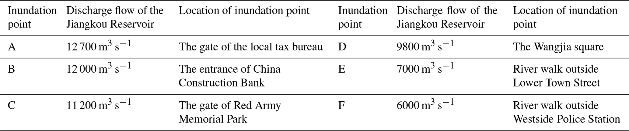
Taking inundation point A as an example, its specific meaning is as follows: when the flood flow reaches 12 700 m³ s⁻¹, the flood will inundate the location of the original tax bureau's main gate. The actual representation of an inundation point is the flood boundary line. The determination of each inundation point is based on historical observations and verification from the flood management department during multiple flood events. During the flood season, personnel from the management department are stationed at these locations to monitor the situation and supervise the evacuation process. The actual flood boundary lines of each inundation point are provided by the local flood disaster management department. We have verified these inundation boundaries via the investigation of historical flood traces and interviews with local residents, and they are used for subsequent inundation simulation validation. The selected flood event is a typical flood process measured by the local hydrological bureau based on the 2005 extreme flood event. This flood process includes flow values corresponding to the six inundation points.

The river in the study area is situated in the lowest part of the terrain, with impermeable roads and various buildings constructed along the slopes on both sides. During a flood, the inundation area rapidly spreads from the river channel towards the riverbanks, with the majority of human and economic losses occurring near the riverbanks. The flood then quickly recedes along the impermeable road surfaces on the slopes of the riverbanks, returning rapidly to the river channel. The impact of the urban drainage network during this process is relatively minor. Additionally, the large Jiangkou Reservoir, located near the study area, significantly blocks sediment from the upstream flow during floods (Winton et al., 2019). The main objective of this study is to assess the impact of the terrain data resolution; therefore, the influence of the urban drainage network and sediment transport is not considered in the flood simulation.

2.2 Drone image acquisition and processing for generating the DSM and DTM

The general workflow for drone image acquisition and processing is outlined in Fig. 2. The drone flight campaign took place on 10 January 2023, during the winter dry season, when the study area experienced low river depths and exposed riverbeds. A DJI Matrice 300 RTK drone equipped with a Ruibo five-lens oblique photography sensor was used for the survey. The DJI Pilot 2 software was employed for flight control, enabling the automatic configuration of flight paths and shooting parameters. In order to minimize the effects of building obstructions within the survey area, the flight altitude was set to 200 m, with image overlaps configured at 80 % in the longitudinal direction and 70 % in the side direction (Cunliffe et al., 2016). A total of 1467 vertical images were captured, achieving a ground sampling distance of 3 cm.

Figure 2 Flowchart of the drone image acquisition and processing.

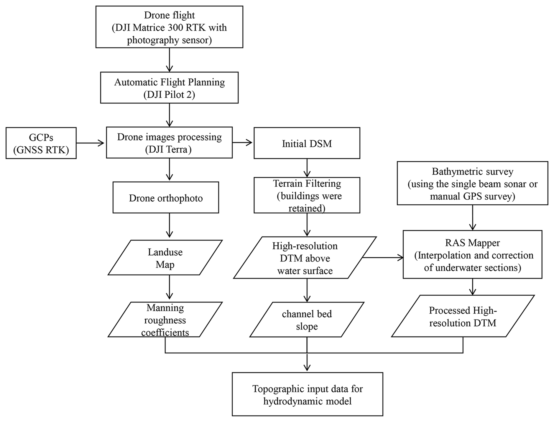
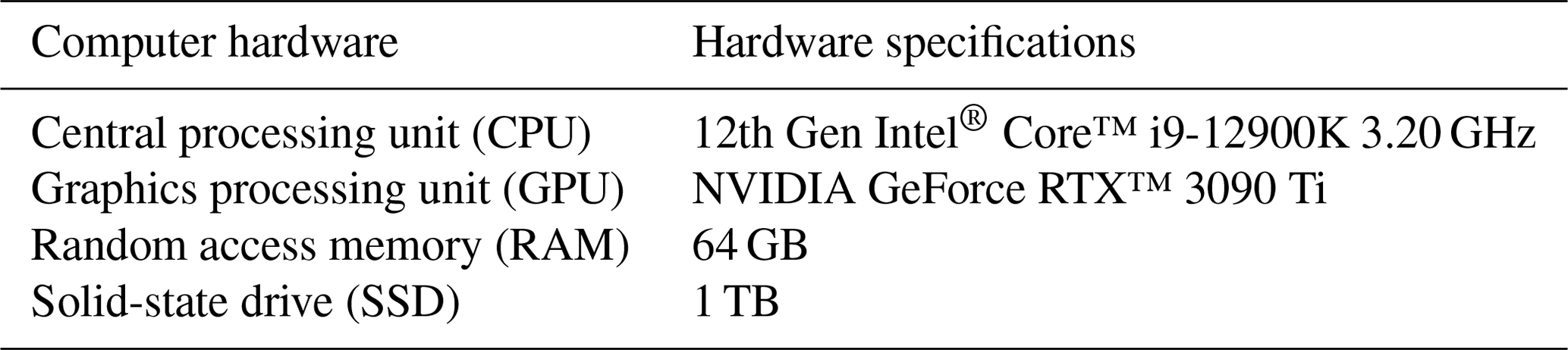
The ground control points (GCPs) were established using a Hi-Target Global Navigation Satellite System (GNSS) receiver in real-time kinematic (RTK) positioning mode. DJI Terra software was utilized to process the drone images, incorporating five control points to optimize sensor position and orientation data and to verify positional accuracy. The final output products included orthoimages and an initial DSM. To ensure the preservation of spatial details, the “highest-quality” processing option was selected when using DJI Terra to process the imagery (i.e., selecting the highest point cloud density and feature points). This option imposes certain requirements on the computer hardware. The hardware specifications used in this study are shown in Table 2, and the initial DSM accuracy achieved was 6 cm.

Table 2 List of computer hardware.

A DSM (digital surface model) represents the elevation data of all visible surface features, including vegetation, buildings, and overhead power lines. To achieve accurate hydraulic modeling, it is typically necessary to filter out these surface features from the DSM to generate a DTM (digital terrain model), which focuses only on the natural terrain without surface features. In this study, PCI Geomatica software was used to filter vegetation, water surfaces, and noise from roads in the initial DSM. All buildings along the riverbank were preserved to meet the requirements for flood inundation simulation. PCI Geomatica allows manual local editing of the DSM, which is a better option for our study area, as the vegetation is relatively small and dispersed. Compared to global filtering of the entire study area, local processing is more suitable and results in higher DTM accuracy. The specific processing workflow is as follows:

• Step 1. Import the initial DSM, open the DEM editor, and create a new polygon layer. Select the local area to be filtered (Fig. 3a).

• Step 2. Select the average filter to smooth the local area and initially reduce noise effects, making the filtered area transitions more natural.

• Step 3. Use the pit and bump filter, selecting remove bump and remove pit to filter local undulations and bumps in the area, mainly targeting mid- to low-elevation vegetation and noise on exposed riverbeds. This step requires alternating between remove bump and remove pit multiple times, adjusting the filter parameters (size and gradient, which control the size and shape of the objects to be filtered) appropriately. The parameters are gradually adjusted from large to small until the filtered area becomes smooth and shows no further changes (Fig. 3b).

• Step 4. Apply the terrain filter to remove residual visible features that are difficult to filter, such as taller vegetation. Terrain filters focus on overall topographic features, and as buildings are retained for flood inundation simulation, care should be taken to avoid selecting buildings when filtering the area (Fig. 3c).

• Step 5. Use the median filter to smooth rough edges from the previous steps. This step will not remove any remaining bumps or pits.

• Step 6. After filtering one area, select the next area and repeat the steps above until all noise, except buildings along the riverbank, has been filtered out. The final output is the DTM that can be input into the hydraulic model.

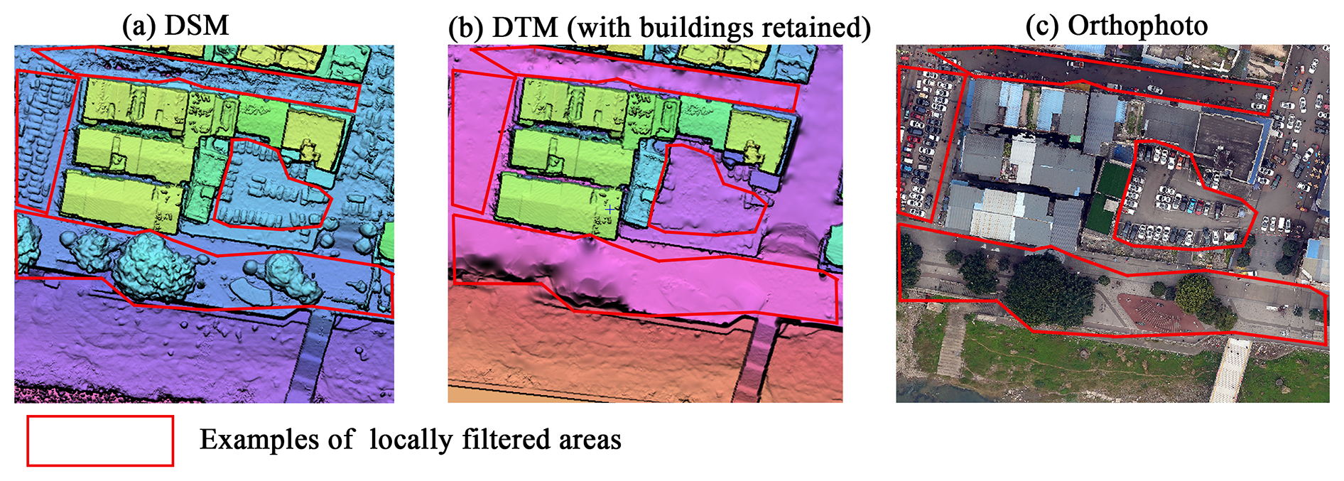
Figure 3 Visualization of the DTM generation from a DSM using PCI Geomatica: (a) the DSM, (b) the DTM, and (c) an orthophoto.

The DTM was subsequently resampled to coarser resolutions of 1, 5, 10, 15, and 30 m for further analysis.

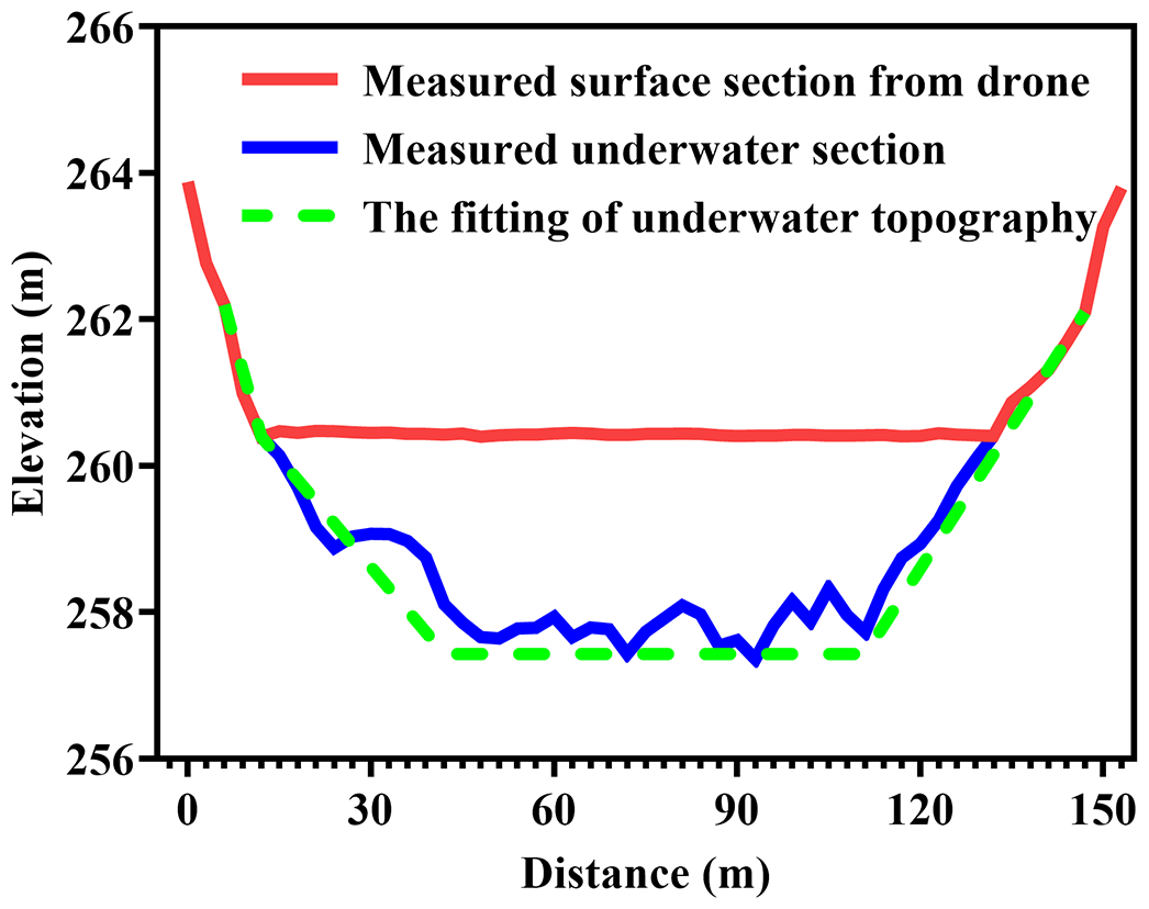
Traditionally, in shallow-water areas, bathymetric measurements are taken by operators using a RTK-GNSS receiver while wading through the water. In deeper waters, bathymetric measurements are typically conducted using sonar instruments mounted on crewed or uncrewed vessels. Research using drone-borne sensors for bathymetric measurements has also made significant progress, such as drone-borne ground-penetrating radar or blue–green lidar. Although these methods require certain conditions with respect to the water depth and clarity, they have demonstrated superior performance to traditional sonar methods in specific scenarios, showing substantial potential in practical applications (Bandini et al., 2023; Mandlburger et al., 2020; Bandini et al., 2018; Pan et al., 2015). In this study, measurements were conducted during the winter low-flow period, when river depths were shallow and large areas of riverbed were exposed. As such, uncrewed boats equipped with single-beam sonar were used to measure underwater cross-sections in the non-dried sections of the river.

Based on the research of Zhao et al. (2017), during the dry season, drone imagery could be used to capture the downward trend in the exposed river floodplains on both sides of the river cross-section. By integrating the measured water depths, the underwater cross-sections of the river were generalized into rectangular, trapezoidal, or arc-shaped profiles (Fig. 4). The complete underwater terrain data were then obtained through cross-section interpolation. This interpolation correction was carried out using the terrain-processing tool RAS Mapper in the Hydrologic Engineering Center's River Analysis System (HEC-RAS) model. The tool uses linear interpolation to modify the underwater terrain between the measured cross-sections and generate a new terrain model. This terrain model can then be combined with the general surface terrain model (which does not accurately depict the terrain below the water surface) to create an improved terrain model for hydraulic modeling and mapping (U.S. Army Corps of Engineering, 2016).

Figure 4 Generalization of the underwater cross-section.

2.3 Flood inundation modeling

The hydraulic model used in this study is HEC-RAS (version 6.3.1). HEC-RAS is developed by the Hydrologic Engineering Center of the U.S. Army Corps of Engineers (U.S. Army Corps of Engineering, 2016). This software allows one to perform 1D steady-flow and 1D and 2D unsteady-flow hydraulics modeling, sediment transport and mobile bed computations, water temperature modeling, and generalized water quality modeling (U.S. Army Corps of Engineering, 2016). It is one of the most widely used hydraulic models globally that is publicly available. This model includes two computational solvers, the 2D Saint-Venant equations (Eq. 1) and the 2D diffusion-wave equation (Eq. 2). The vector forms of the momentum equations are as follows:

$$\begin{array}{}\text{(1)}& {\displaystyle }\begin{array}{rl}{\displaystyle \frac{\partial \mathit{V}}{\partial t}}& +\left(\mathit{V}\cdot \mathrm{\nabla }\right)\mathit{V}+f_{\mathrm{c}}\mathit{k}\times \mathit{V}=-g\mathrm{\nabla }{z}_{\mathrm{s}}+{\displaystyle \frac{\mathrm{1}}{h}}\mathrm{\nabla }\cdot \left({\mathit{\nu }}_{t}h\mathrm{\nabla }\mathit{V}\right)\\ & -{\displaystyle \frac{{\mathit{\tau }}_{\mathrm{b}}}{\mathit{\rho }R}}+{\displaystyle \frac{{\mathit{\tau }}_{\mathrm{s}}}{\mathit{\rho }h}}-{\displaystyle \frac{\mathrm{1}}{\mathit{\rho }}}\mathrm{\nabla }{p}_{\mathrm{a}},\end{array}\text{(2)}& {\displaystyle \frac{g{n}^{\mathrm{2}}}{R^{\mathrm{4}/\mathrm{3}}}}\left|\mathit{V}\right|\mathit{V}=-g\mathrm{\nabla }{Z}_{\mathrm{s}}-{\displaystyle \frac{\mathrm{1}}{\mathit{\rho }}}\mathrm{\nabla }{p}_{\mathrm{a}}+{\displaystyle \frac{{\mathit{\tau }}_{\mathrm{s}}}{\mathit{\rho }h}}.\end{array}$$

Here, $\mathit{V}={\left(u,v\right)}^T$ is the velocity vector (m s⁻¹); ν_t is the horizontal eddy viscosity coefficient tensor (m² s⁻¹); ∇ is the gradient operator (1 m⁻¹); k is the unit vector in the vertical direction (dimensionless); τ_b and τ_s are the bottom shear and 9 wind surface stress vector (kg m s⁻²), respectively; h is water depth (m); f_c is the Coriolis parameter (1 s⁻¹); p_a is atmospheric pressure (kg m s⁻²); R is the hydraulic radius (m); Z_s is the water surface elevation (m); g is gravitational acceleration (m/ s⁻²); n is the Manning roughness coefficient (s m${}^{-\mathrm{1}/\mathrm{3}})$; and ρ is water density (kg m⁻³).

The 2D unsteady-flow equation solvers both use the implicit finite-volume solution algorithm. The implicit solution algorithm allows for a larger computational time step than explicit methods. Compared with traditional finite-difference and finite-element techniques, the finite-volume method significantly improves the stability and robustness of the solution process (Mourato et al., 2021). For specific model introductions and usage, please refer to the “HEC-RAS Applications Guide” and “HEC-RAS User's Manual” (U.S. Army Corps of Engineering, 2016).

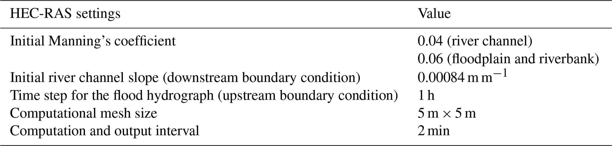
The flood inundation modeling in this study used a full 2D unsteady-flow model. Figure 5 shows the topographic data of the area, the 2D computational grid, and the upstream and downstream boundary conditions (represented by the blue line in Fig. 5). For the model's upstream boundary, the input data consisted of a typical flood hydrograph with a time step of 1 h. The downstream boundary conditions were defined using the normal water depth, calculated based on the river slope. The downstream river slope, derived from the drone-obtained DTM, was determined to be 0.00084 m m⁻¹. The detailed model setup is presented in Table 3.

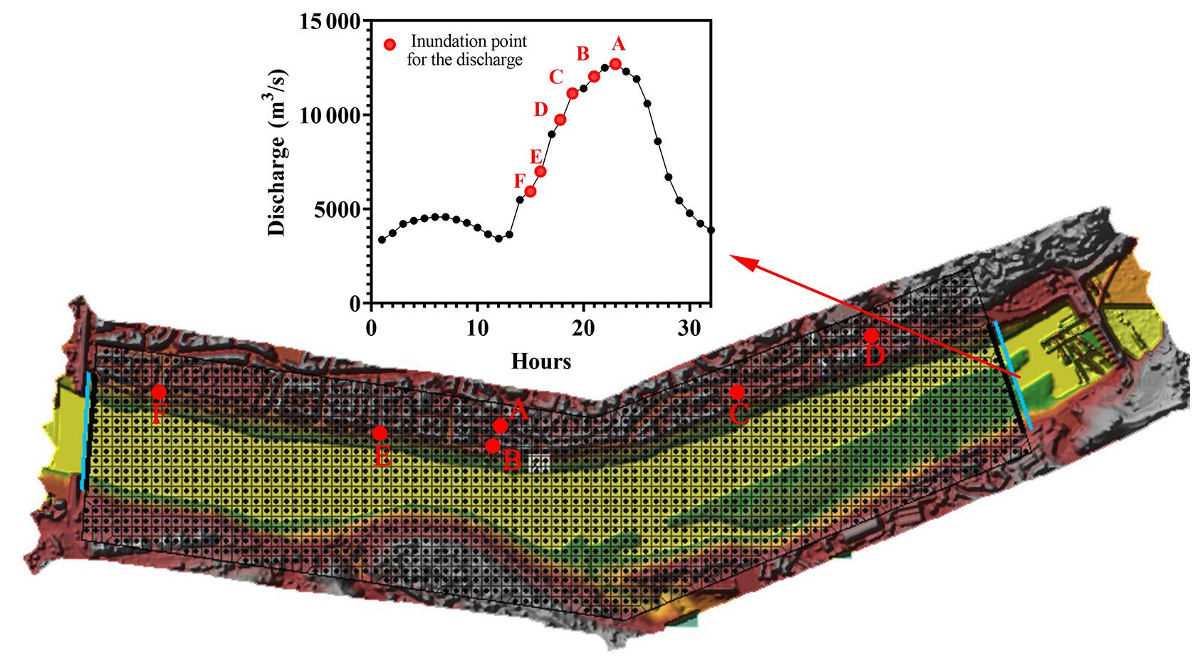
Figure 5 Mesh used for all simulations with the 6 cm DTM in the HEC-RAS model and the hydrograph of the typical flood event.

Table 3 The HEC-RAS model settings.

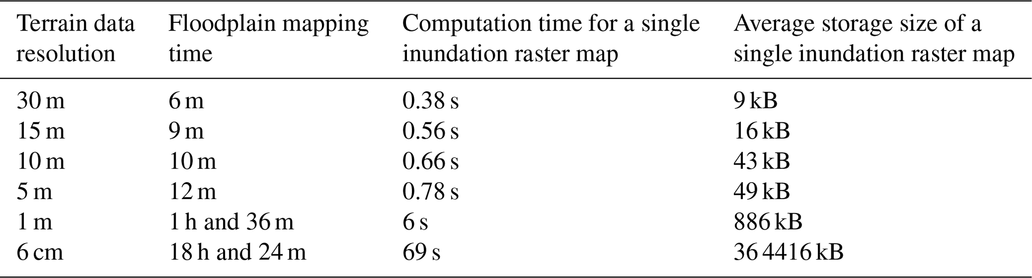
The computational time for 2D flood inundation simulations using HEC-RAS is primarily related to two factors: the 2D flow calculation and floodplain mapping. The computational time for 2D flow is associated with the computational mesh size setting and is less influenced by the resolution of the terrain data. Yalcin (2020) found that significant fluctuations in the results of the 2D flow calculations only appear when the computational mesh size exceeds 15 m × 15 m. Given that the main objective of this study is to assess the impact of the DTM resolution, a computational mesh with 5 m × 5 m cells was used for all simulations. In contrast, floodplain mapping is based on terrain data, and its computational efficiency and drawing accuracy are directly related to the DTM resolution. Selecting an appropriate DTM resolution is crucial for the timeliness and reliability of flood risk analysis. Table 4 shows the computational results for floodplain mapping using different DTM resolutions, and the hardware specifications used for the simulations are shown in Table 2.

Table 4 The computational time for floodplain mapping and the storage size of the inundation raster map.

2.4 Topographic attributes analysis

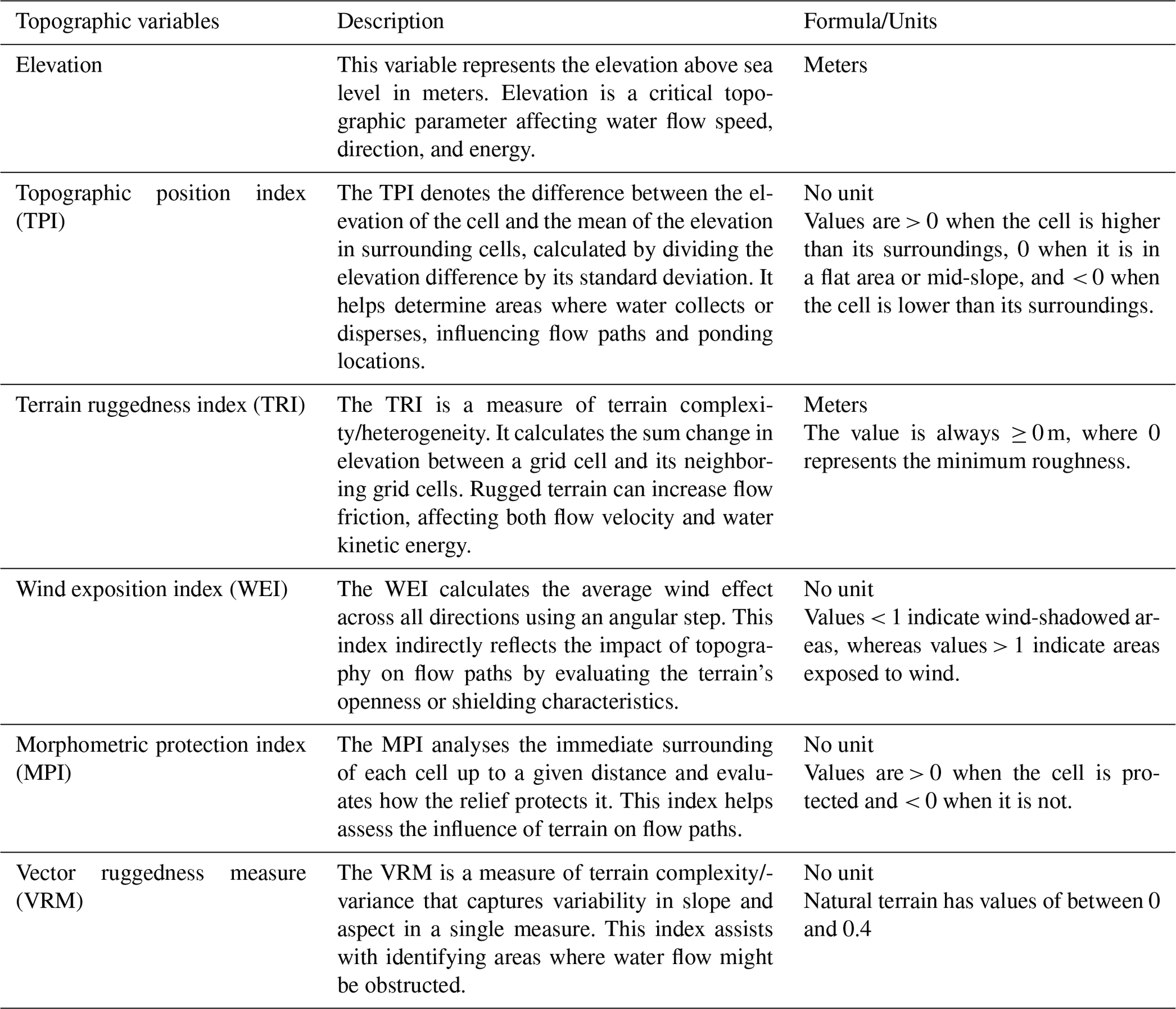
Obtaining topographic attributes from digital terrain data is a common approach used to capture digital terrain features, evaluate terrain data quality, and analyze the uncertainty in a terrain representation at different resolutions. More than 10 commonly used topographic attributes are employed in various fields such as hydrological analysis, land use, and soil–vegetation studies. Each indicator uses different methods to describe the terrain structure and shape, and the undulation of the terrain directly affects the flow of water on the surface. In this study, six topographic attributes closely associated with hydraulic simulation and hydrological analysis were selected to evaluate the effects of DTMs at different resolutions on flood inundation simulation. The topographic attributes are as follows: the elevation, the topographic position index (TPI), the terrain ruggedness index (TRI), the wind exposition index (WEI), the morphometric protection index (MPI), and the vector ruggedness measure (VRM). The detailed definitions of these attributes are shown in Table 5.

Table 5 Description of topographic variables used as independent explanatory variables for modeling. Descriptions are based on Salekin et al. (2021), Harris and Baird (2019), and the SAGA-GIS Tool Library Documentation (v8.5.1).

Salekin et al. (2023) demonstrated that, when extracting topographic attributes, using the average value across the plot is more representative than directly measuring the center point, as the latter lacks spatial representativeness. Therefore, this study established 894 square plots of 30 m × 30 m in the analysis area based on the coarsest resolution (30 m) as the plot side length. This approach ensures that the calculation of the plot contains complete grid pixels at the coarsest resolution and that each plot can contain multiple complete grid pixels at a finer resolution. All geospatial processing and data extraction were performed using ArcGIS and the System for Automated Geoscientific Analyses (SAGA v8.5.1) (Conrad et al., 2015). The mean absolute error (MAE) was used to analyze the differences in the DTM topographic attributes at different resolutions:

$$\begin{array}{}\text{(3)}& \mathrm{MAE}={\displaystyle \frac{\mathrm{1}}{m}}{\sum }_{i=\mathrm{1}}^m\left|x_i-y\right|,\end{array}$$

where m is the total number of plots calculated; x_i is the average value of the topographic indicators of each plot in the resampled DTM; and y is the topographic attribute value as a benchmark and control value, i.e., the value of topographic attributes of the 6 cm DTM obtained by the drone.

3 Results and discussion

3.1 Performance of the drone DTM in urban fluvial flood modeling of mountainous regions

For most flood events, obtaining real, accurate, and complete flood inundation maps (including inundation extent and flood depth) for model validation is highly challenging. In this study, six inundation warning points provided by the local flood disaster management department were used for validation. Based on (1) the years of manual observations made by management department personnel at these points during the flood season and (2) the investigations of historical flood traces and interviews with local residents, the historical flood inundation boundary lines for each point were delineated (Fig. 6). The six images on the inner side of Fig. 6 are field survey images of the six inundation points. The red lines in the images represent the delineated historical inundation boundaries, which were used to validate the simulated flood inundation extent (i.e., to assess whether the simulated flood boundary coincides with the red historical inundation boundary). During the simulation process, in order to ensure accurate representation at the six inundation points, a 20 % upward adjustment was made to the Manning coefficient for both the river channel and the riverbanks.

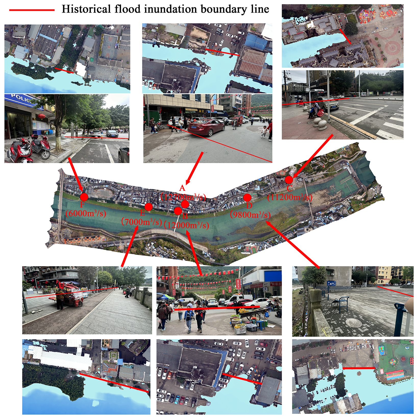
Figure 6 Comparison and validation of inundation point simulation results with historical flood boundary lines. The inner six images are on-site survey images of the six inundation points, whereas the outer six localized magnified orthophotos are the corresponding flood mapping results from HEC-RAS.

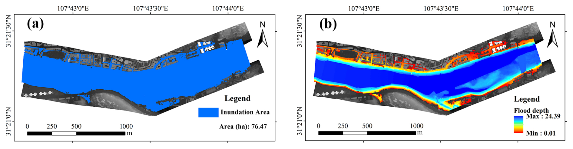
Figure 7 The flood simulation results for the maximum flood peak flow based on the 6 cm DTM: (a) inundation area and (b) inundation depth.

The flood simulation results based on the 6 cm DTM are shown in Figs. 6 and 7. The six localized magnified orthophotos in the outer part of Fig. 6 represent the corresponding flood mapping results from HEC-RAS at the six inundation points. The red lines in the localized magnified orthophotos are consistent with the red lines in the field photos. From the HEC-RAS 2D simulation results, the simulated flood inundation at the six points aligns well with the historical flood inundation boundary lines. As the elevation positions of the six inundation points increase with the corresponding flood flow values, and their distribution covers the upper, middle, and lower sections of the study area, this indicates good agreement between the flood simulation based on high-precision terrain data (6 cm DTM) and the actual flood inundation. Therefore, the calibrated model results obtained with the 6 cm DEM are considered to be benchmark conditions for subsequent spatial and statistical comparative analysis based on different resolutions. The final benchmark flood inundation area was 76.47 ha, with a maximum flood depth of 24.39 m, a minimum depth of 0.01 m, and an average depth of 18.09 m (Fig. 7)

3.2 Effects of different resolutions on flood modeling

3.2.1 Overall comparison of flood area and depth

The resampled DTMs (1, 5, 10, 15, and 30 m) were sequentially input into HEC-RAS for flood inundation modeling. The simulation results were compared with the benchmark (6 cm DTM), both spatially and statistically. The inundation area of the benchmark was overlaid with the inundation boundary polygons from simulations based on other resolutions for comparative analysis. For inundation depth, the ArcGIS raster calculator was used to output the difference between the inundation depth raster maps, enabling pixel-by-pixel comparisons. The pixel-based differences (i.e., errors) were then used to evaluate the simulation performance based on DTMs of different resolutions, using statistical metrics such as the mean absolute error (MAE) and root-mean-square error (RMSE). Figure 8 shows the spatial and statistical comparison of flood inundation from simulations at different DTM resolutions with the benchmark (6 cm DTM) under maximum flood peak flow conditions (12 700 m³ s⁻¹).

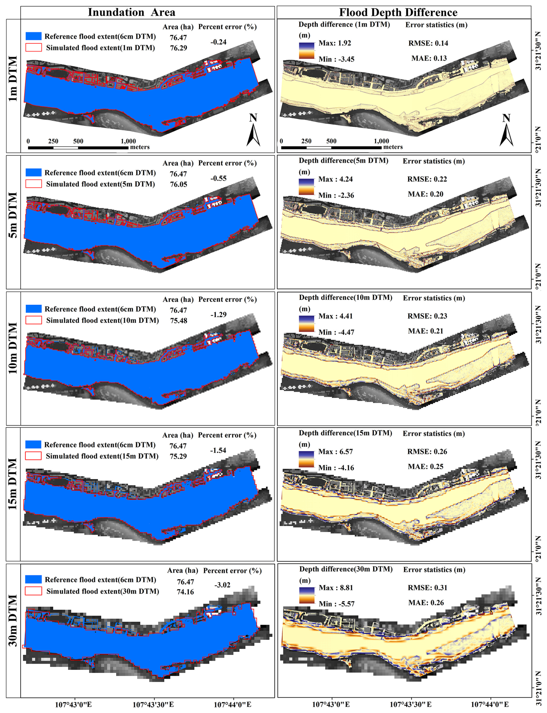
Figure 8 Spatial and statistical analyses of the effects of the DTM resolution on the simulated inundation extent and flood depth by comparison with benchmark conditions (6 cm DTM).

As shown in Fig. 8, as the DTM resolution decreases, the inundation area shows a decreasing trend compared to the benchmark, especially when using a 10 m DTM or coarser-resolution DTMs, where noticeable differences in inundation extent appear on the riverbanks outside the main river channel. Many areas of significant flood extent mismatch are evident. For flood depth difference, the discrepancies become more pronounced when using 10 and 15 m DTMs. This observation is supported by both statistical values and the clear spatial distribution changes. Additionally, the flood depth difference shows varying degrees of change both within the main river channel and along the floodplain and riverbanks.

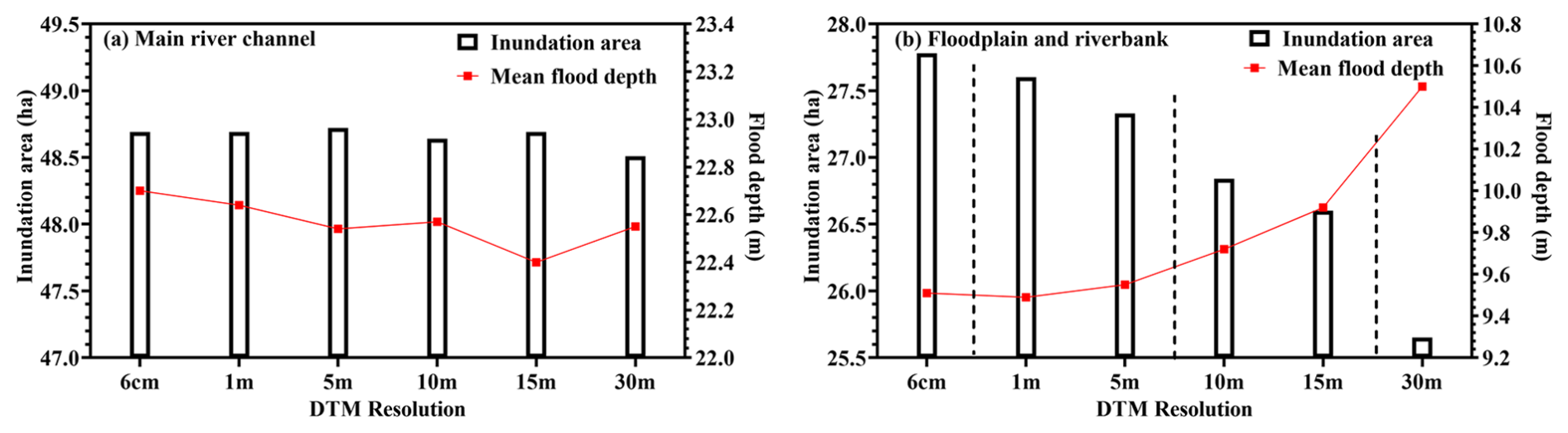
Figure 9 Trend in the inundation area and mean flood depth derived from DTMs with different resolutions at the flood peak for the (a) main river channel and (b) floodplain and riverbank (out of the main river channel).

Figure 9 shows the variation trend in inundation area and mean flood depth at maximum flood peak flow (12 700 m³ s⁻¹) based on DTMs at different resolutions. As shown in Fig. 9a, within the main river channel, there is no distinct trend in the inundation area as the DTM resolution decreases, with only slight fluctuations observed. In contrast, the mean flood depth shows an obvious fluctuation when the resolution is greater than 5 m. The absence of significant trends in the modeling results within the main channel can be attributed to the coarsest resolution (30 m) being much smaller than the average river width (around 182 m) in the study area. Meanwhile, except for the exposed riverbed topographic data obtained by drone during the dry season, the rest of the underwater topography of the river channel was obtained by generalized cross-section interpolation based on the trend in the floodplain (obtained by the drone) combined with the maximum underwater depth (obtained by the uncrewed boat), which has a limited capture of the undulating features of the underwater topography, resulting in insensitivity to DTM resolution changes in the main river channel inundation simulation. Although no clear change pattern emerges, the fluctuations in the results indicate that the impact of the DTM resolution on the flood inundation simulation is not a simple linear relationship.

As shown in Fig. 9b, the floodplain and riverbank areas outside the main channel exhibit a notable decreasing trend in inundation area as the DTM resolution decreases. Using the flood modeling result from the 6 cm DTM as a benchmark, the inundation area decreases by 0.65 %, 1.62 %, 3.38 %, 4.25 %, and 7.67 % for DTM resolutions of 1, 5, 10, 15, and 30 m, respectively. In contrast, the mean flood depth remains relatively unchanged at 1 and 5 m DTMs, and a clear increasing trend is observed beyond 5 m resolution, with the mean flood depth rising by 2.21 %, 4.31 %, and 10.41 % at DTM resolutions of 10, 15, and 30 m, respectively. Overall, both the inundation area and mean flood depth exhibit distinct step changes. Specifically, compared to the benchmark, the magnitude of change is minimal and similar at 1 and 5 m DTM resolutions, more substantial yet similar at 10 and 15 m DTM resolutions, and greatest at 30 m DTM resolution. The dashed lines in Fig. 9b were used to better depict the variations (step changes) between the simulation results at different resolutions.

In the floodplain and riverbank areas of the mountainous city, the simulated inundation area decreases as the DTM resolution decreases, whereas the mean flood depth increases. This indicates that changes in resolution significantly affect the characterization of DTM topography. Notably, both the flood area and depth showed some stage changes in the whole mountainous urban fluvial flood modeling (as shown in Fig. 9), and this was also supported by visualizing the inundation area at different DTM resolutions (Fig. 6). The possible reason for this phenomenon is that, as the resolution becomes coarser, the topographic undulation of the inundation area changes from the original smooth trend to a step-like trend, altering the flood inundation process in the model. This step-like trend in topographic undulation also makes the relationship between the resolution change and flood inundation characteristics present a nonlinear relationship (step change). As the resolution decreases beyond a certain threshold, these step-like changes in topography can become increasingly pronounced.

3.2.2 Specific effects of different resolution the inundation points

To further analyze the effect of the DTM resolution on urban fluvial flood modeling of mountainous regions, we evaluated the simulation results at six inundation points across different DTM resolutions. As an example, Fig. 10 illustrates the inundation modeling results at point C (11 200 m³ s⁻¹) produced using different DTM resolutions. The inundation scenario simulated with the 6 cm DTM was treated as the benchmark for comparison, with the red line in Fig. 10 representing the benchmark inundation boundary lines. By comparing the modeling results of different resolutions at point C, the simulations based on the 1 and 5 m DTMs demonstrated the best alignment with the benchmark boundary, with nearly identical inundation extents. In contrast, the simulations using the 15 and 30 m DTMs showed poorer performance, as the modeled inundation boundaries deviated significantly from the benchmark. The inundation boundary simulated using the 10 m DTM slightly exceeds the boundary line of the benchmark. While the boundaries nearly coincided, the modeled flood depth at 10 m resolution was greater than the benchmark (the color is deeper than the benchmark).

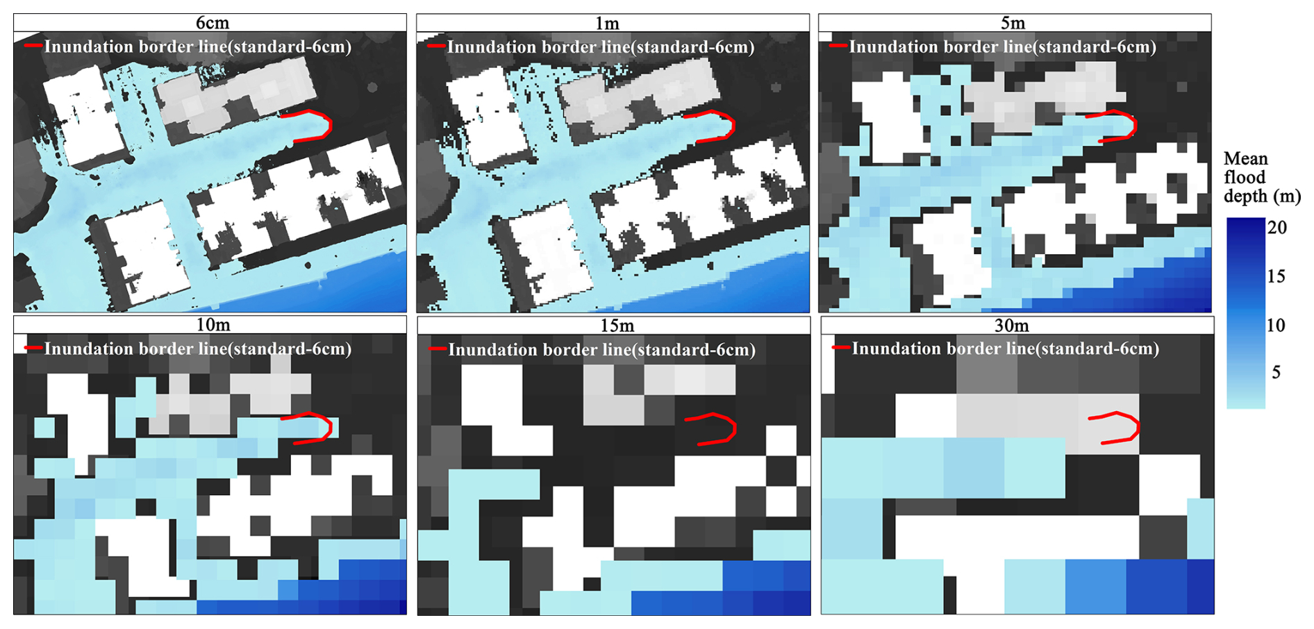
Figure 10 Inundation modeling results at point C (11 200 m³ s⁻¹) produced using DTMs with different resolutions.

Using the inundation border lines of the six inundation points simulated with the 6 cm DTM (represented by the red lines in Fig. 8) as the benchmark, the red benchmark lines were converted into points based on the flood inundation depth raster maps using ArcGIS. Each point corresponds to the flood depth value of the associated pixel. These points were then used to extract the corresponding flood depth from the flood inundation depth raster maps at different resolutions (if a point falls on a grid cell with no inundation data, the flood depth is set to zero). The pixel-based flood depths were subtracted from the benchmark flood depths to calculate the mean error. Table 6 presents the comparison of simulation results at six inundation points using DTMs of different resolutions with the benchmark, with the values in the table representing the average error in flood depth between the simulated inundation boundaries and the benchmark.

Table 6 Modeling results of the inundation boundary and flood depth at six inundation points using DTMs with different resolutions.

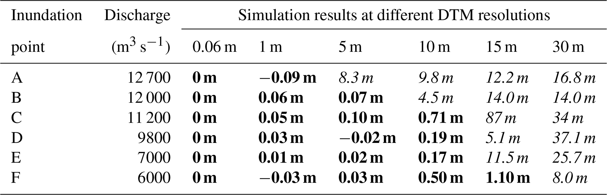
Note that bold font indicates that the simulated inundation boundary is in coincidence with the benchmark boundary, and the numbers indicate the average error between the simulated inundation boundary's flood depth and the benchmark; italic font indicates that the simulated inundation boundary is not in coincidence with the benchmark boundary, and the numbers indicate the average distance by which the simulated inundation boundary differs from the benchmark.

A horizontal comparison of the results in Table 6 reveals that the influence of DTM resolution on the accuracy of inundation simulation becomes more pronounced as the simulated discharge increases. For the minimum discharge of 6000 m³ s⁻¹ (point F), the inundation boundaries simulated using DTMs ranging from 1 to 15 m resolution align closely with the benchmark boundary (bold font in the table). However, at the maximum discharge of 12 700 m³ s⁻¹ (point A), only the simulation result using the 1 m DTM is in agreement with the benchmark. For those points at which the simulated inundation boundary does not coincide with the benchmark, the average distance between the simulated boundary and the reference boundary generally increases as the resolution becomes coarser.

A vertical comparison of simulation results at different resolutions (Table 6) indicates that the inundation boundary simulated using a 1 m DTM is in perfect coincidence with the benchmark, exhibiting minimal error in flood depth with an average error of 0.04 m. The inundation boundaries produced using 5 and 10 m DTMs are basically consistent with the benchmark at all inundation points except at some extreme discharges, but the flood depth simulated using a 10 m DTM is much greater than the depth at finer resolutions. When 5 and 10 m DTMs are utilized to determine the qualified inundation border, the average flood depth errors are 0.048 and 0.392 m, respectively. It is clear that DTMs of 15 and 30 m cannot meet the requirements for urban fluvial flood modeling of mountainous regions.

Considering the results presented in Fig. 10 and Table 6, it can be seen that the simulation effect of flood characteristics shows a certain step change with the change in DTM resolution in urban fluvial flood modeling of mountainous regions. Specifically, when the resolution is greater than 10 m, the simulation results of its flood characteristics cannot meet the requirements for accurately modeling flood inundation in riverside mountainous cities. When the resolution is maintained at or below 5 m, the simulation outcomes largely fulfill the necessary criteria, with the results from a 1 m DTM aligning closely with those derived from centimeter-level DTM simulations. Although the results obtained using a 10 m DTM are generally acceptable with respect to inundation boundaries, they tend to overestimate flood depth compared to the simulations conducted with 1 and 5 m DTMs.

3.3 Analyzing the causes of effects based on topographic attributes

Floods in mountainous riverside cities are mainly caused by the rapid confluence of flash floods driven by heavy rain. To further analyze the fundamental reasons for the impact of different DTM resolutions on flood inundation simulation of mountainous riverside cities, six topographic attribute indicators, namely, elevation, the TPI, the TRI, the WEI, the MPI, and the VRM, were selected to statistically analyze the topographic attributes of DTMs at different resolutions. Table 7 presents the statistical results of the topographic features derived from the 6 cm DTM, reflecting the topographic undulation of the study area from multiple perspectives. For example, the TPI quantifies the height difference between a grid cell and the average height of its surrounding grid cells, with values ranging from −2.87 to 28.51 and an average close to 0. This indicates significant topographic variation in the area, characterized by distinct distributions of elevated and depressed landforms. The filtered DTM retains buildings for flood modeling, so variables such as the WEI, the MPI, or the VRM, which describe steep ridge sites as well as accumulation areas, can also be used to characterize the DTM's representation of buildings and bare ground in mountainous areas.

Table 7 Summary of the topographic attribute index values for the standard (6 cm) DTM.

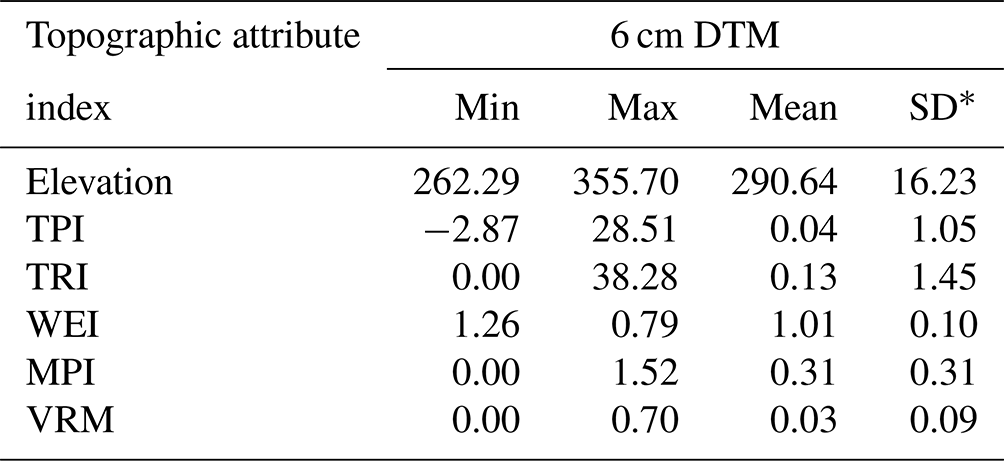
^* SD represents standard deviation.

Table 8 Mean absolute error (MAE) of six topographic attribute metrics at different resolutions.

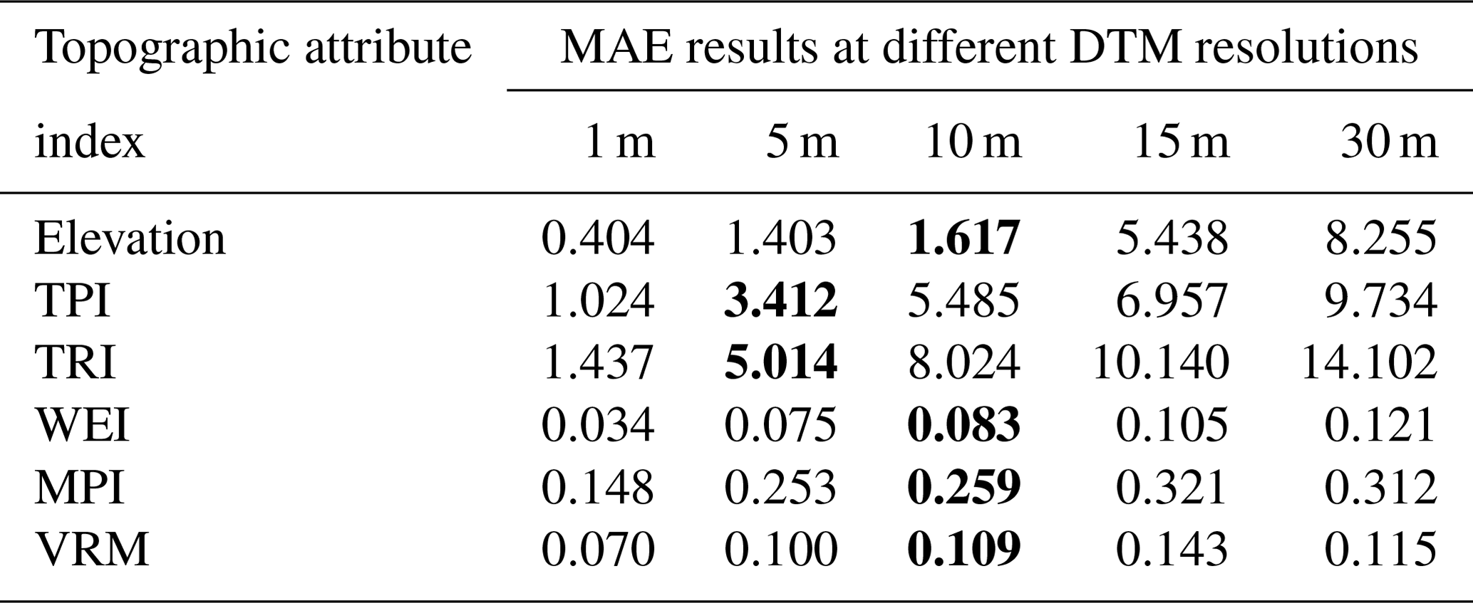
Note that bold font indicates abrupt/step changes before and after the value.

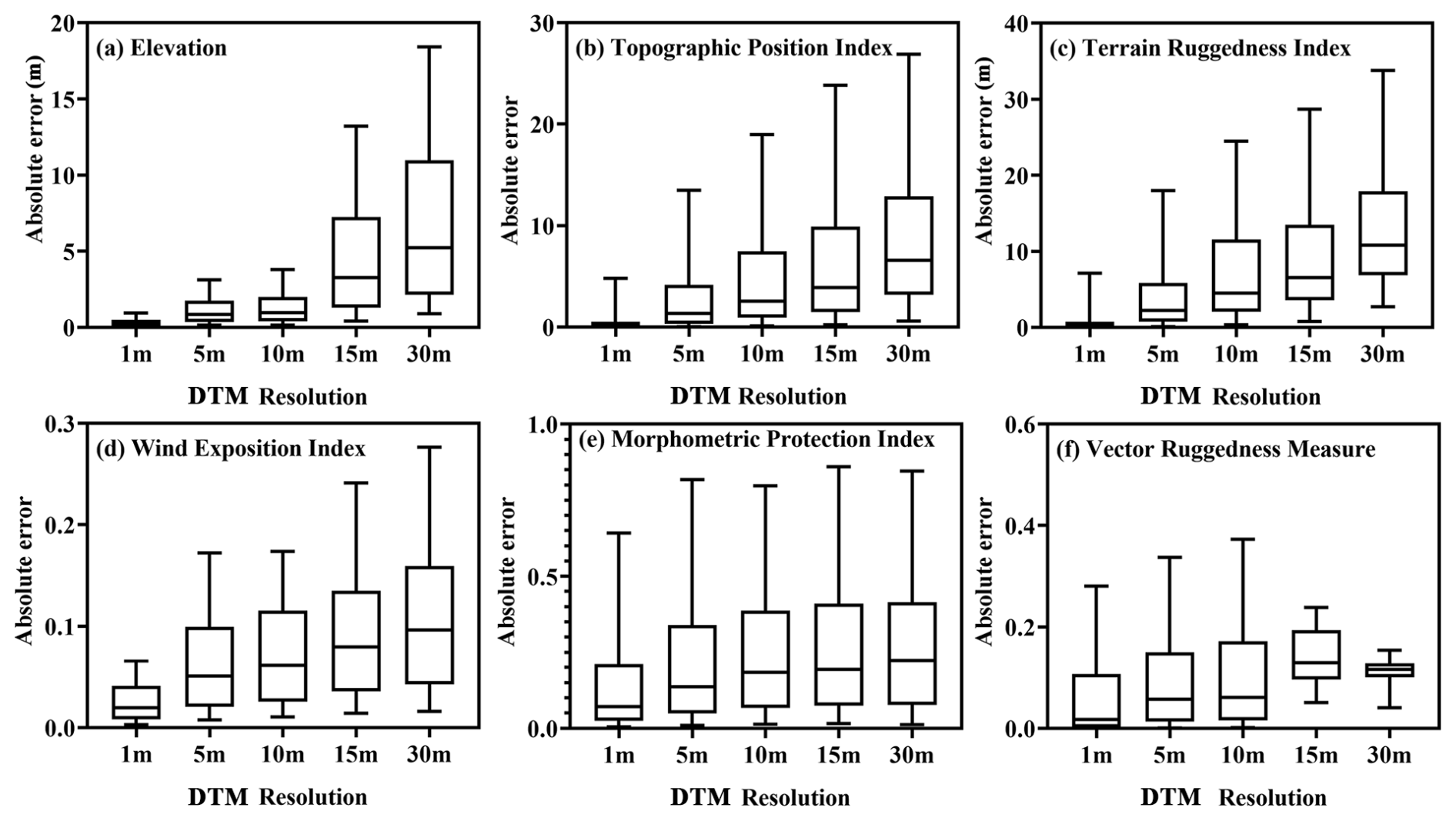
Figure 11 Variations in absolute errors for topographic features derived using DTMs with different resolutions.

Using the topographic attributes derived from the 6 cm DTM as a benchmark, this study analyzed the characterization of topographic attributes in the study area as represented by DTMs with resolutions ranging from 1 to 30 m. Figure 11 illustrates the distribution of absolute errors for the six topographic attribute metrics calculated across 894 square plots, while Table 8 presents the final mean absolute error (MAE) values. The results show that the overall error between the six topographic attribute indicators and the benchmark increases as the resolution of the DTM becomes coarser. As shown in Fig. 9a, d, e, and f, the four indicators (elevation, the WEI, the MPI, and the VRM) exhibit a significant step change around a resolution of 10 m, with errors for the 5 and 10 m DTMs being relatively similar. However, for the remaining two indicators (the TPI and TRI), the error associated with the 10 m DTM is substantially greater than that associated with the 5 m DTM. This discrepancy suggests the existence of a threshold with respect to the effects of DTM resolution changes on topographic attributes. DTMs with resolutions below 10 m are more effective in capturing the undulating features of the topography in the study area, which is critical for accurately modeling the inundation area. However, for features characterized by specific elevation differences, such as the TPI and TRI, it is advisable to maintain a resolution of 5 m or finer, as this will directly influence the accuracy of flood depth modeling.

In conjunction with the earlier analysis of flood inundation simulations, it was found that there is consistency between the simulation results of flood inundation characteristics and the changes in topographic attributes as the resolution changes. This consistency indicates that the effect of DTM resolution on inundation modeling is mainly related to the complexity and undulation of the terrain, and the simulation accuracy is directly related to whether the DTM can accurately capture topographic features. The analysis of topographic attributes provides theoretical support for obtaining an optimal resolution to match simulation requirements. For urban fluvial flood modeling of mountainous regions utilizing a DTM obtained by drones as the terrain input, a resolution within 10 m can basically meet the simulation needs of the inundation area, as a DTM with this resolution can accurately characterize the features of the undulating and complex terrain (including buildings). However, considering the simulation needs of the flood depth and balancing the computational cost and the simulation requirements, a resolution of 1–5 m can present better results, as a DTM with this resolution can accurately capture the characteristics of the specific difference in elevation.

4 Conclusion

This study conducted a 2D flood inundation simulation for a mountainous riverside city in Southwestern China, utilizing a high-precision DTM obtained by drone. Considering the local government's flood prevention plan, field investigation of historical inundation traces, and inundation boundaries, the flood inundation simulation area and six inundation points for model validation were determined. The results showed that the flood inundation simulation and the historical flood inundation boundary lines at the six inundation points were well matched, and there was good consistency between the model simulation results and the actual flood inundation.

The 6 cm DTM obtained by drone was resampled into 1, 5, 10, 15, and 30 m DTMs, respectively, as the terrain input for the 2D flood inundation simulation, and the effect of different resolutions on urban fluvial flood modeling of mountainous regions was discussed. The results showed that, on the floodplain and riverbank outside the main channel, the inundation area showed a significant decreasing trend with the decrease in resolution. The mean flood depth did not change significantly when using a 1 and 5 m DTM, but it showed a significant increasing trend after the resolution was greater than 5 m. The area both inside and outside of the river channel showed a certain step change.

Similarly, based on the 6 cm DTM as the benchmark, the characterization of topographic attributes by DTMs with different resolutions was further analyzed. We found that there was a certain threshold for the effect of DTM resolution on topographic attributes. Compared with a DTM with a resolution of more than 10 m, a DTM with a resolution of less than 10 m could better capture the undulating and complex terrain features of the study area, especially within 5 m.

According to the analysis of terrain attributes using a DTM obtained by drone to conduct urban fluvial flood modeling of a mountainous region, the resolution of the terrain data used should be kept within 1–5 m. However, if larger watersheds and larger mountainous cities were involved, in the case of non-extreme discharges, considering the cost of acquisition and processing, using a resolution of 5–10 m could also meet certain requirements in terms of inundation area drawing, but there could be the possibility of the overestimation of flood depth.