Technical note: An approach for handling multiple temporal frequencies with different input dimensions using a single LSTM cell

Long short-term memory (LSTM) networks have demonstrated state-of-the-art performance for rainfall-runoff hydrological modelling. However, most studies focus on predictions at a daily scale, limiting the benefits of sub-daily (e.g. hourly) predictions in applications like flood forecasting. Moreover, training an LSTM network exclusively on sub-daily data is computationally expensive and may lead to model learning difficulties due to the extended sequence lengths. In this study, we introduce a new architecture, multi-frequency LSTM (MF-LSTM), designed to use input of various temporal frequencies to produce sub-daily (e.g. hourly) predictions at a moderate computational cost. Building on two existing methods previously proposed by the co-authors of this study, MF-LSTM processes older inputs at coarser temporal resolutions than more recent ones. MF-LSTM gives the possibility of handling different temporal frequencies, with different numbers of input dimensions, in a single LSTM cell, enhancing the generality and simplicity of use. Our experiments, conducted on 516 basins from the CAMELS-US dataset, demonstrate that MF-LSTM retains state-of-the-art performance while offering a simpler design. Moreover, the MF-LSTM architecture reported a 5 times reduction in processing time compared to models trained exclusively on hourly data.

1 Introduction

Data-driven methods, particularly long short-term memory (LSTM) networks (Hochreiter and Schmidhuber, 1997), have demonstrated state-of-the-art performance in rainfall-runoff hydrological modelling (Kratzert et al., 2019b; Lees et al., 2021; Loritz et al., 2024). Currently, most studies primarily focus on predictions at a daily scale. However, certain applications, such as flood forecasting, can benefit from sub-daily scale predictions, especially in small fast-responding catchments. These higher temporal resolutions allow the model to better capture an event's magnitude and avoid artificial attenuation or dampening caused by daily aggregation. In addition, they allow the model to reproduce more accurately the temporal dynamics of the hydrograph and open up the possibility of capturing flash floods. For this reason, many operational flood forecasting services, including the National Water Prediction Service of the National Oceanic and Atmospheric Administration (NOAA) in the USA and the Flood Forecasting Centre of Baden-Württemberg (HVZ) in Germany, produce forecasts at a sub-daily resolution for their operational services.

One major drawback of running LSTM models at exclusively hourly resolution is the significant increase in computational cost for both model training and evaluation. For instance, studies using LSTM models at daily resolution typically employ a sequence length of 365 d for predictions (Kratzert et al., 2019b; Klotz et al., 2022; Lees et al., 2021; Loritz et al., 2024). By spanning a full year of data, this approach allows the LSTM model to capture long-term seasonal processes, such as snowmelt (Kratzert et al., 2019a). However, for hourly data, the equivalent sequence length increases to $\mathrm{365}\times \mathrm{24}=\mathrm{8760}$ time steps, leading to a substantial increase in the computational resources required. Moreover, LSTM models have shown difficulties in learning information over long sequence lengths (Chien et al., 2021; Zhang and You, 2020), which would create a direct limitation when working exclusively with high-frequency data, such as hourly or 15 min resolutions.

A potential strategy for tackling this problem is to reduce the sequence length. However, this comes at the cost of excluding long-term processes. For example, if a sequence length of 365 time steps is maintained when working with hourly data, the look-back period would only cover 2 weeks, as opposed to a full year. Consequently, the model might not account for important long-term dynamics.

Another possible solution is the concept of ordinary differential equation LSTM (ODE-LSTM) models proposed by Lechner and Hasani (2020). The authors handle non-uniformly sampled data through the use of a continuous-time state representation of recurrent neural networks. Gauch et al. (2021) carried out experiments exploring the potential of ODE-LSTM models in rainfall-runoff modelling. However, they indicated that this method achieved lower performance at a higher computational time than their proposed alternative.

Gauch et al. (2021) proposed the idea of processing older inputs at coarser temporal resolutions compared to more recent data. This approach is based on the fact that, for a dissipative system like a catchment, the importance of the temporal distribution of inputs diminishes the further back in time we look (Loritz et al., 2021). For instance, in cases where discharge during spring is driven by snowmelt, the exact hour in which snow accumulated 2 months earlier is unlikely to affect the hydrograph. Similarly, when modelling a storm, the basin's response will vary depending on the soil saturation. If the soil is saturated due to heavy rain over the past month, the precise timing of a peak in rainfall 3 weeks before becomes irrelevant. Thus, this approach to handling inputs at different temporal resolutions allows the model to capture long-term processes without the computational burden of processing all data at high frequency. In the following, we use a concrete example to both better illustrate the ideas proposed by Gauch et al. (2021) and make the connection with our method. For this, we will use 1 year of data to make a prediction, but only the most recent 2 weeks ($\mathrm{14}\times \mathrm{24}=\mathrm{336}$ time steps) will be processed at hourly resolution, while the rest will be processed at daily resolution. The number of time steps processed at each frequency is a model hyperparameter.

The first architecture proposed by Gauch et al. (2021), referred to as shared multi-timescale LSTM (sMTS-LSTM), begins with a forward pass at daily resolution (e.g. 365 time steps). The LSTM network's hidden and cell states from 2 weeks prior to the final time step are then retrieved, and the LSTM network is re-initialized with these states. Then, a second forward pass is performed using hourly data for the last 2 weeks. Moreover, since both daily (from the first forward pass) and hourly (from the second forward pass) predictions are available for the last 2 weeks, the authors proposed a regularization technique in which an extra term is incorporated into the loss function to induce consistency between the daily and hourly predictions.

One limitation of this architecture, highlighted by the authors, is that, because the same LSTM cell processes both daily and hourly data, the input at both timescales must include the same number of variables. As they mentioned, this can be problematic in operational settings, where different temporal resolutions often have different available variables. To address this, the authors proposed a more general architecture called multi-timescale LSTM (MTS-LSTM). In this variant, the hidden and cell states retrieved from 2 weeks prior are passed through a transfer function, and the result is used to initialize a second LSTM cell, which processes the hourly data. The advantage of this approach is that, with separate LSTM cells for each temporal frequency, different sets of input variables can be used at each resolution. We refer the reader to Fig. B1 for a graphic visualization of these ideas.

Building on the work of Gauch et al. (2021), we propose a new methodology that combines the strengths of both models. We refer to it as multi-frequency LSTM (MF-LSTM). On the one hand, this new methodology retains the simplicity and elegance of the sMTS-LSTM model by using a single LSTM cell to process data at multiple temporal frequencies. On the other hand, we keep the ability of the MTS-LSTM model to handle different numbers of input variables at each frequency, which we accomplish through the use of embedding layers. Moreover, and as explained in detail in the following sections, we make predictions only at the highest frequency (e.g. hourly), and the remaining frequencies are recovered by aggregation, which guarantees cross-timescale consistency without the use of additional regularization.

The remainder of the paper is structured as follows. Section 2 details the MF-LSTM architecture and the experimental setup, including the datasets used and the benchmark comparisons. In Sect. 3, we present and analyse the results of these experiments. Finally, Sect. 4 summarizes the key findings and offers the study's conclusions.

2 Data and methods

2.1 Data and benchmarking

To ensure consistency with Gauch et al. (2021) and to enable a direct comparison, we followed their experimental setup. Keeping the same experimental setup allowed us to compare their results against our proposed method without having to rerun their experiments. The importance of driving model improvement through community benchmarks has been discussed previously in the machine learning and hydrological communities (Donoho, 2017; Nearing et al., 2021; Klotz et al., 2022; Kratzert et al., 2024).

The experiments were conducted in 516 basins located across the contiguous United States, all of which are part of the CAMELS-US dataset (Addor et al., 2017). From this dataset, we extracted 26 static attributes (see Table A3). The hourly input data (see Table A1) were extracted from North American Land Data Assimilation System (NLDAS-2) hourly products (Xia et al., 2012), while the target discharge data were retrieved from the USGS Water Information System (USGS, 2016). Following standard machine learning practices, the data were divided into three subsets. The training period was from 1 October 1990 to 30 September 2003, the validation period was from 1 October 2003 to 30 September 2008, and the testing period was from 1 October 2008 to 30 September 2018.

2.2 MF-LSTM

The concept of MF-LSTM comes from the principle that an LSTM cell has no inherent limitation in processing data at different temporal frequencies. In contrast to process-based hydrological models, where one would not update a storage (say interflow) with a 5 mm h⁻¹ flux (say evapotranspiration) in one time step and then with an 8 mm d⁻¹ flux in another, an LSTM cell can accommodate an equivalent updating scheme. To process an input, an LSTM cell always processes a sequence one step at a time. However, there is no explicit assumption about the progress of time within one such step. Due to its time-dependent gating mechanisms, the LSTM cell can learn to modulate how the cell states are updated, regardless of the temporal resolution of the inputs. Consequently, we can leverage this property to handle multiple temporal frequencies within a single LSTM cell, processing older inputs at coarser resolutions and more recent data at higher resolutions.

A concrete example of this approach is illustrated in Fig. 1a using daily and hourly frequencies. In this example, our goal is to predict hourly discharge. To capture long-term processes, we initially input a full year of high-resolution hourly data (e.g. $\mathrm{365}\times \mathrm{24}=\mathrm{8760}$ hourly time steps). To avoid the computational burden and learning difficulties associated with processing long sequences, the first n time steps were processed at a coarser resolution, reducing the length of the input sequence entering the LSTM cell. The number of time steps processed at each resolution is a model hyperparameter and can be determined through hyperparameter tuning.

The example in Fig. 1a shows the case where the first $n=\mathrm{351}\times \mathrm{24}=\mathrm{8424}$ time steps were aggregated into 351 blocks, each containing an average of 24 hourly measurements. Given the normalization of the input and target data and the non-mass-conservative structure of the LSTM model, both the average and the sum of the hourly measurements can be used. The remaining $m=\mathrm{14}\times \mathrm{24}=\mathrm{336}$ time steps were then processed at the original hourly resolution. By applying this method, we reduced the original sequence length from 8760 to $\mathrm{351}+\mathrm{336}=\mathrm{687}$ time steps, decreasing the amount of data to be processed by a factor of 12.8.

To inform the LSTM cell about the frequency it should be operating at, we added a flag channel. This has a value of zero for the first 351 time steps and a value of one for the remaining 336. Adding a flag to help the model distinguish between different types of conditions is a common practice in machine learning, as it provides the model with additional context (Nearing et al., 2022). For the LSTM cell specifically, the flag channel acts as an additional bias that further regulates the gating mechanisms. Figure 1b shows the inclusion of the flag channel for the different frequencies.

Note that, in the previous paragraph, we used pre-defined values to simplify the explanation and clarify the concept. However, the method is by no means restricted to this setup, and its flexibility allows it to adjust the number of time steps processed at each resolution and the order in which the different frequencies are applied. Additionally, the composition of the time series can be alternated from batch to batch during training or inference. Moreover, the method is not restricted to using only two frequencies and, as we show in the next section, a weekly–daily–hourly frequency scheme can be handled without any additional burden.

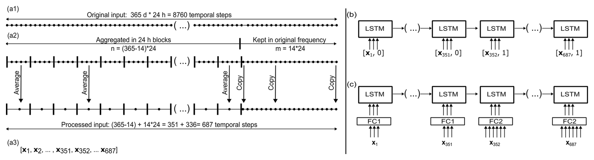
Figure 1 Data-handling structure for MF-LSTM. (a1) The original sequence length consists of 1 year of hourly data: 8760 temporal steps. (a2) The first $(\mathrm{365}-\mathrm{14})\times \mathrm{24}=\mathrm{351}\times \mathrm{24}=\mathrm{8424}$ time steps are aggregated into 351 blocks, while the remaining $\mathrm{14}\times \mathrm{24}=\mathrm{336}$ time steps are processed at their original hourly frequency. (a3) The final input series that will be processed by the LSTM cell consists of $\mathrm{351}+\mathrm{336}=\mathrm{687}$ time steps. (b) In the case where the same number of inputs for each frequency are available, we add a flag as an additional channel to help the LSTM cell to identify each frequency. (c) In the case where different numbers of inputs for each frequency are available, a fully connected (FC) linear layer can be used to map the variable number of inputs of each frequency to a pre-defined number of channels.

One of the main advantages stated by Gauch et al. (2021) about the MTS-LSTM architecture is its ability to handle a variable number of inputs for each frequency, because different LSTM cells are used for each temporal frequency (see Fig. B1). We propose the use of embedding networks as an alternative solution. By using one embedding network for each temporal frequency, we can map different numbers of inputs to a shared dimension. This strategy allows us to separate the steps of our pipeline. We use the LSTM cell for sequence processing only, and we use the embedding networks to prepare the original information in the format or type that the LSTM cell requires. In the simplest case, the embedding networks could even be a single linear layer, as will be used for the rest of this paper (see Fig. 1c). We evaluated the embedding network with and without the flag channel and observed comparable performance in both cases. This result indicates that the embedding network can internally identify frequency information without the need for an additional flag channel. Therefore, we opted for the simpler approach and excluded the extra channel.

In summary, the main distinction between MF-LSTM and sMTS-LSTM lies in MF-LSTM's ability to handle a different number of inputs for each temporal frequency, which gives an advantage in operational settings where different temporal resolutions often have different available variables. Moreover, the primary difference between MF-LSTM and MTS-LSTM lies in the simpler architecture of the former, which uses a single LSTM cell, in contrast to one cell per frequency. This results in a more parsimonious model that aligns closely in structure and usage with traditional single-frequency LSTM models.

3 Results and discussion

3.1 Performance comparison

Our long-term goal, which goes beyond the scope of this study, is to implement an operational hourly hydrological forecasting system using machine learning methods. The MF-LSTM method is a step towards achieving this, as it enables computationally efficient simulation of hourly discharges while allowing us to handle a variable number of inputs at each temporal resolution – both requirements for our broader objective. Consequently, the results reported in this section will focus on two aspects: the ability of MF-LSTM to produce hourly discharge and the ability to handle a variable number of inputs while doing so.

Gauch et al. (2021) presented two experimental setups that address these aspects. Therefore, we ran these experiments as a benchmark to evaluate the performance of our method against their results. Both experiments evaluate the case in which one is interested in simulating hourly discharges, and they do so by processing part of the information at daily frequency and part of it at hourly frequency. More specifically, data for 1 year are processed, but only the last 14 d (336 h) are processed at hourly frequency. The value of 336 h was identified in the original study by hyperparameter tuning. In all of the cases, the results are reported using an ensemble of 10 independent LSTM models that were initialized using different random seeds. The final simulation value is taken as the median streamflow across the 10 models for each time step.

The first experiment evaluated the scenario where the same number of inputs (see Table A1) was used for both daily and hourly processing. In this case, we can directly compare our model's performance with the results reported by Gauch et al. (2021) for MTS-LSTM and sMTS-LSTM, together with what they refer to as the naive approach. The naive approach involves running a standard LSTM model exclusively on hourly data with a sequence length of 4320 h (6 months). We can see from Fig. 2a that all the models present the same performance up to the second decimal place, with a median Nash–Sutcliffe efficiency (NSE) of 0.75.

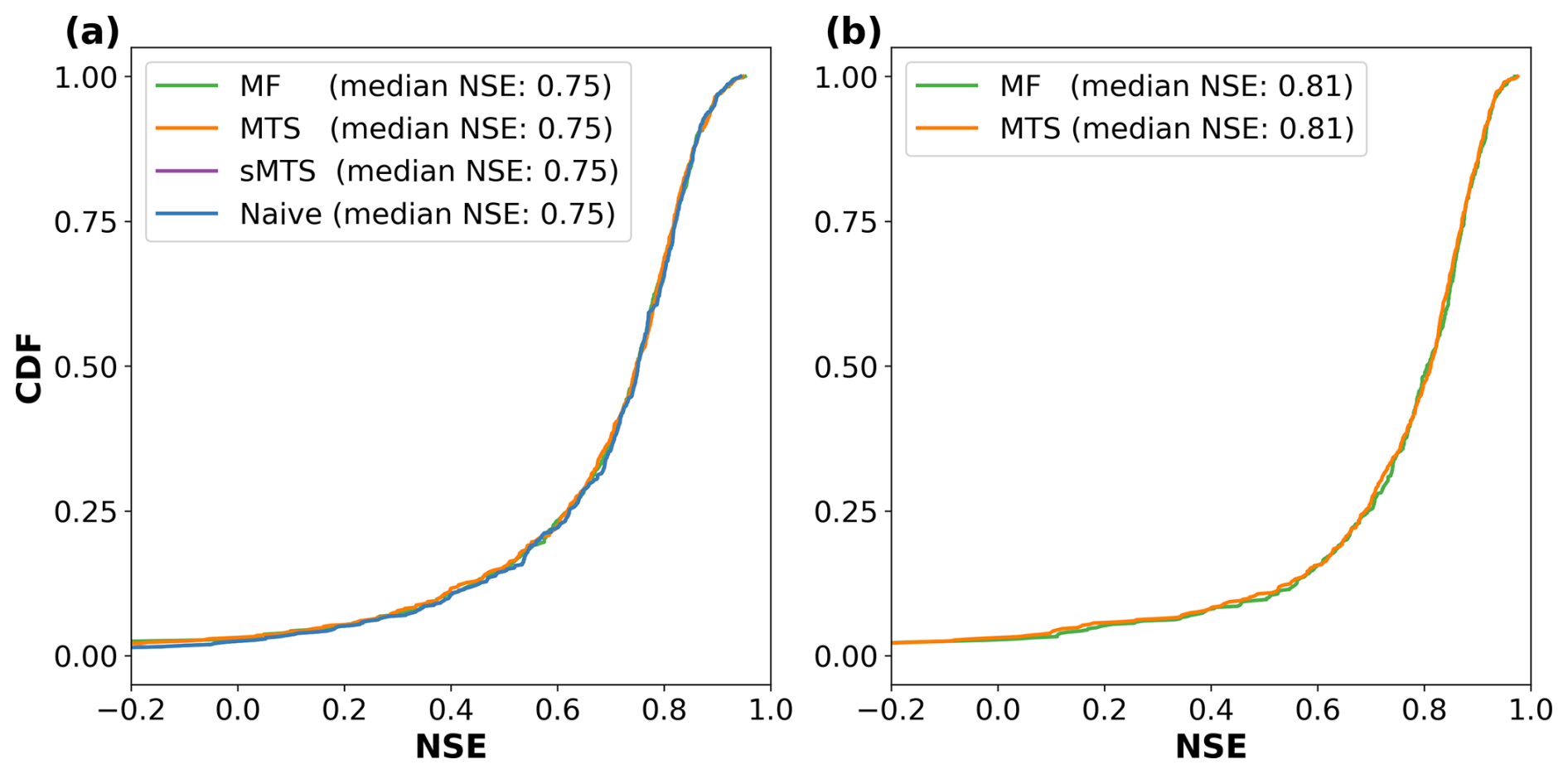
Figure 2 Cumulative NSE distribution of the different models, evaluating the prediction accuracy for hourly discharges along 516 basins in the USA. (a) Case where the same number of variables is used during daily and hourly processing (see Table A1). (b) Case where different numbers of variables are used during daily and hourly processing (see Table A2).

The second experiment evaluated the scenario in which different numbers of inputs were used for the daily and hourly steps (see Table A2). Specifically, the daily frequency incorporated 10 dynamic variables from the Daymet and Maurer forcing datasets, while the hourly steps included 21 variables. Eleven of these variables were sourced from the NLDAS-2 forcing at hourly resolution, and the remaining 10 were a low-resolution re-discretization of the 10 daily variables into an hourly frequency (i.e. the daily value was repeated 24 times). Consistent with Gauch et al. (2021), since the Maurer forcings go until 2008, the results of this experiment are reported for the validation period. As shown in Fig. 2b, MF-LSTM achieves a performance comparable to that of MTS-LSTM, with both reporting a median NSE of 0.81. Comparisons with the sMTS and naive models are not possible for this experiment, as previously explained, because these models cannot accommodate different numbers of variables for different frequencies.

The previous experiments showed that the MF-LSTM architecture can achieve a state-of-the-art performance that is fully comparable with the MTS-LSTM and sMTS-LSTM architectures. The results show that a single LSTM cell can handle multiple temporal frequencies at the same time. Moreover, the second experiment confirms that a simple fully connected linear layer can successfully encode different numbers of input variables in a pre-defined number of channels.

We also ran an additional experiment to evaluate the capacity of the model to handle more than two frequencies. Specifically, we used a weekly–daily–hourly scheme. The first half of the year (182 d) was handled using a weekly aggregation. The next 5.5 months (169 d) were at daily resolution, and the remaining 14 d used an hourly frequency. Our results showed that MF-LSTM is capable of handling this case, presenting a similar performance (see Fig. C1) and reducing the sequence length from 687 to 531.

3.2 Computational efficiency

As shown in Fig. 1a, one key advantage of processing older inputs at coarser temporal resolution than more recent ones is the reduced computational cost, particularly when compared with feeding in the whole sequence length at a finer resolution (e.g. hourly). This reduction in computational cost impacts not only the training time, but also the memory usage. With long sequence lengths, one might run out of GPU memory or be forced to use alternative strategies such as reducing the batch size during training and evaluation.

However, the total training time is influenced by external factors, such as differences in hidden size or batch size, which are not directly related to the methods themselves. To minimize these external effects, we conducted an additional experiment where we standardized the hidden size and batch size across all the models and compared the average time needed to process a batch. The results showed that MF-LSTM, MTS-LSTM, and sMTS-LSTM exhibited nearly identical efficiency, while the naive approach was approximately 5 times slower. For reference, training MF-LSTM on a Tesla V100 GPU took around 7 h.

4 Conclusions

In this study, we introduced the MF-LSTM architecture, designed to produce sub-daily (e.g. hourly) predictions at a moderate computational cost while giving the model access to long sequences of input data. Building on Gauch et al. (2021), our method processes the input's temporal sequence using different aggregations. Hence, it accounts for the fact that the effect of the input's temporal distribution diminishes the further we look back in time. This allows MF-LSTM to predict hourly discharges without the overhead of handling the entire sequence at a fine temporal scale.

The ability of the LSTM model to maintain performance while handling data from the past at lower resolutions highlights how the LSTM cell acts similarly to a process-based hydrological model, with dissipative behaviour when it comes to the memory of past forcings. This is a step towards understanding LSTM-based predictions better as they are gaining popularity for applications in hydrology.

As high-resolution data become increasingly available in the environmental sciences, traditional LSTM models will continue to face challenges when trying to learn from these long sequence lengths. The approach we present here, with its simplicity and computational efficiency, offers a practical solution. Areas like weather forecasting, where data at resolutions of minutes are not uncommon, might benefit from this type of model. Moreover, the possibility of combining multiple frequencies, like our weekly–daily–hourly scheme, enables modellers to extend look-back periods. This may also be beneficial in other domains such as groundwater, where long-term historical data are required to capture slow dynamic processes.

Our proposed embedding strategy opens up the possibility of mapping different numbers of inputs to a shared dimension. This flexibility not only simplifies the model architecture by allowing a single LSTM cell to handle diverse input configurations but also enhances the model's adaptability in operational settings, where the availability of input data may vary across timescales. This overcomes the limitation previously stated in sMTS-LSTM.

Furthermore, we demonstrate that a single LSTM cell can effectively manage processes operating at different timescales (eliminating the need for separate LSTM cells for each timescale) and transfer functions between their hidden states. This results in a more parsimonious model that aligns more closely in structure and usage with traditional single-frequency LSTM models, making the transition from single-frequency to multi-frequency LSTM models more intuitive for users.

Through experiments on 516 basins from the CAMELS-US dataset, the MF-LSTM model demonstrated the same performance as the MTS-LSTM and sMTS-LSTM models, indicating that the added simplicity and generality do not come at the expense of predictive capability. Moreover, the new architecture presents a similar computational cost to the two previous options and reduces the training time by a factor of 5 when compared to the naive approach.

The fact that a single LSTM cell allows us to handle multiple frequencies could be due to the close similarities between processes at different timescales (e.g. daily and hourly). The LSTM architecture takes advantage of these similarities, along with its ability to regulate gates based on the current context, enabling it to effectively process multiple frequencies. By using a single LSTM cell, we can leverage the additional information content encoded in our data.

The hyperparameters of the model were adopted from Gauch et al. (2021), who conducted hyperparameter tuning. We acknowledge that transferring these parameters across different architectures may not guarantee optimal model performance. However, the primary objective of this technical note is to introduce the new architecture. Furthermore, we demonstrate that, even with the given hyperparameters, the proposed model achieves a performance comparable to the current state of the art.

Appendix A: Additional information on the experimental design

The following tables present the variables used in the experiments associated with this study. Tables A1 and A2 present the variables used in the first and second experiments. The third and fourth columns of each table indicate whether the variable was used at daily frequency, hourly frequency, or both. Table A3 shows the 26 static attributes used as additional inputs in the models.

Table A1 Dynamic input variables used in the first experiment, where the same number of variables is used for the daily and hourly frequencies.

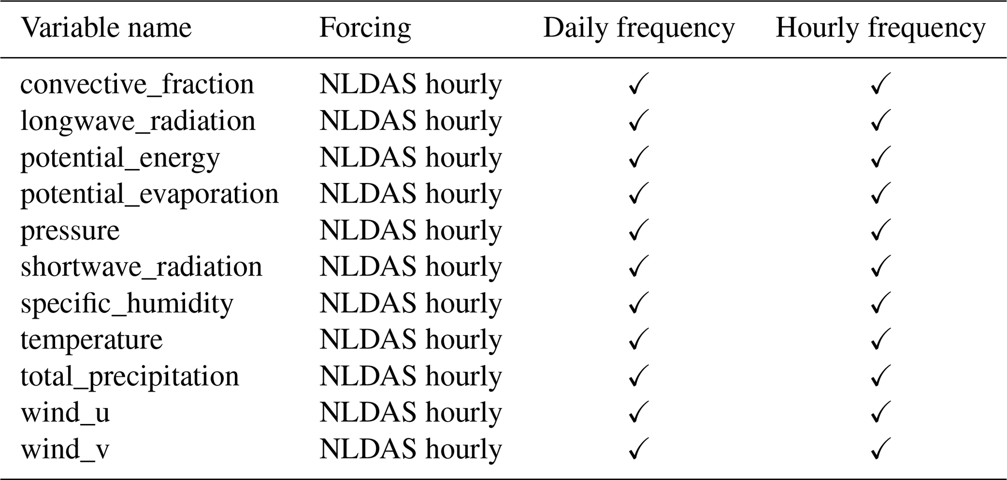
Table A2 Dynamic input variables used in the second experiment, where different numbers of variables are used for the daily and hourly frequencies.

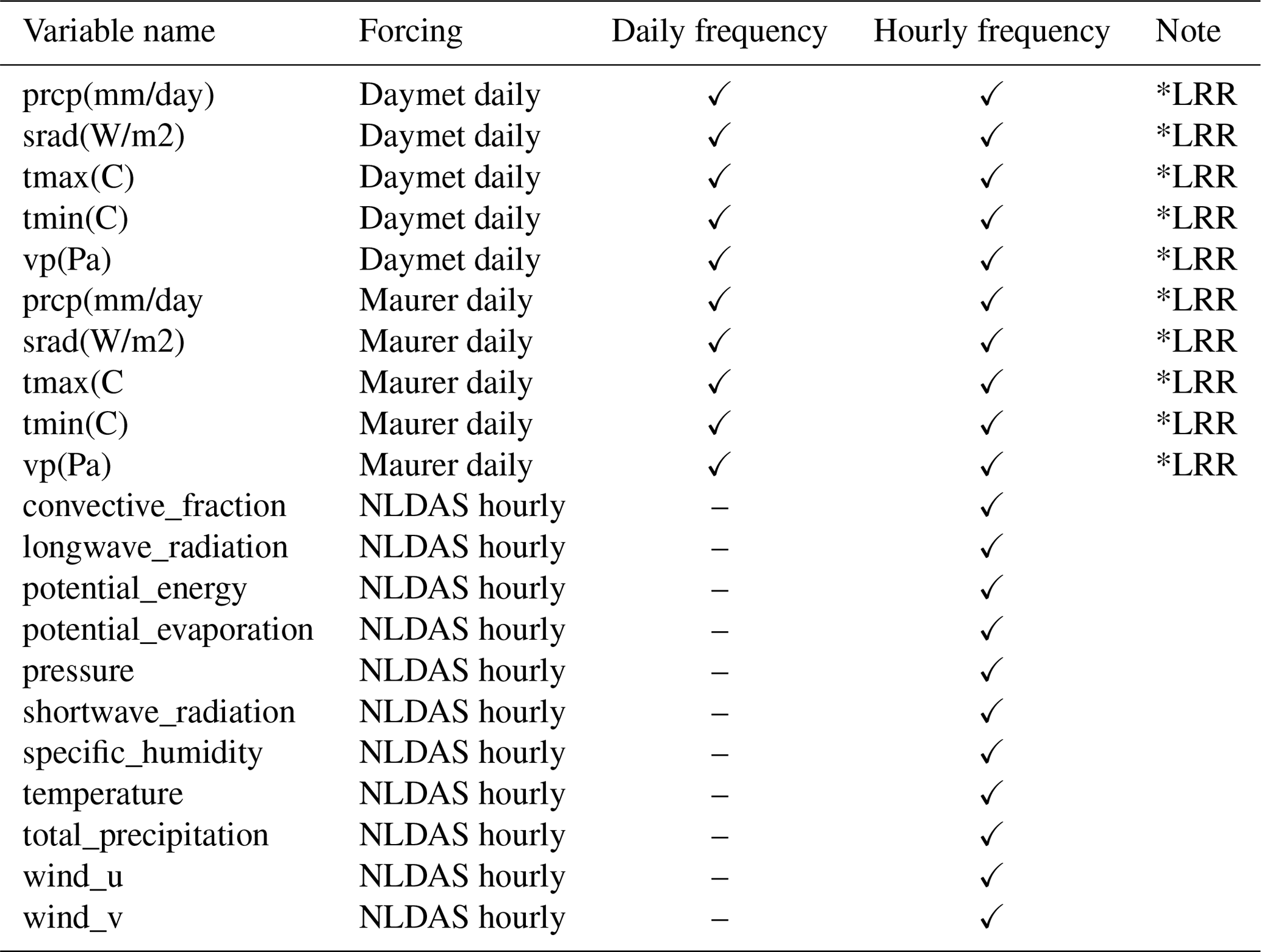
*LRR: low-resolution re-discretization is done when the original daily value is used at hourly frequency. Therefore, the original daily value is repeated 24 times.

Table A3 Names of the 26 static attributes used in the experiments.

Appendix B: Structure of the MTS-LSTM model architecture

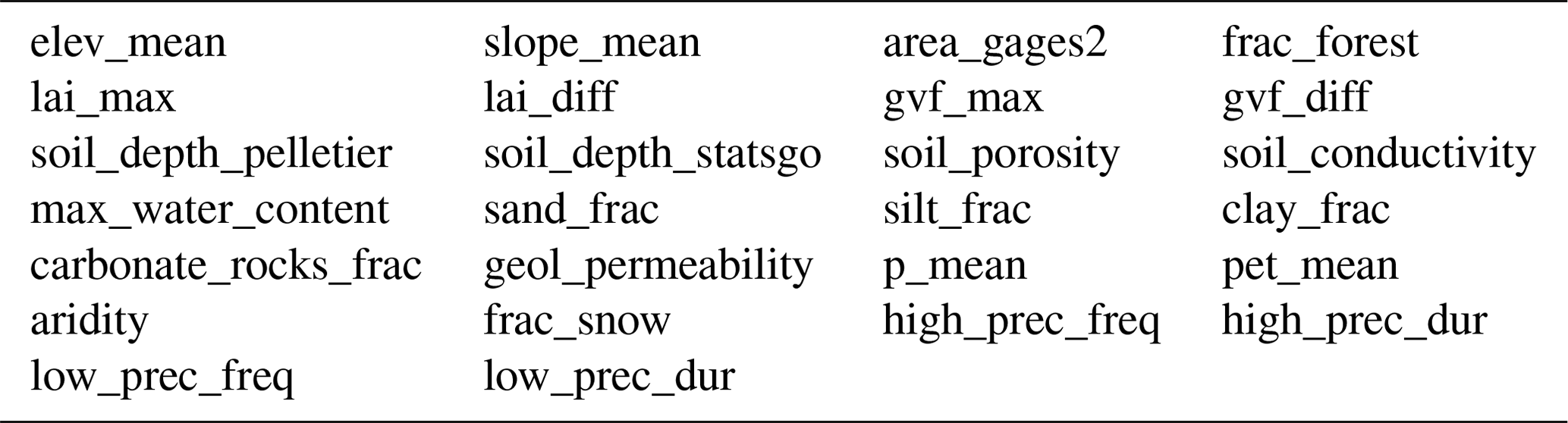
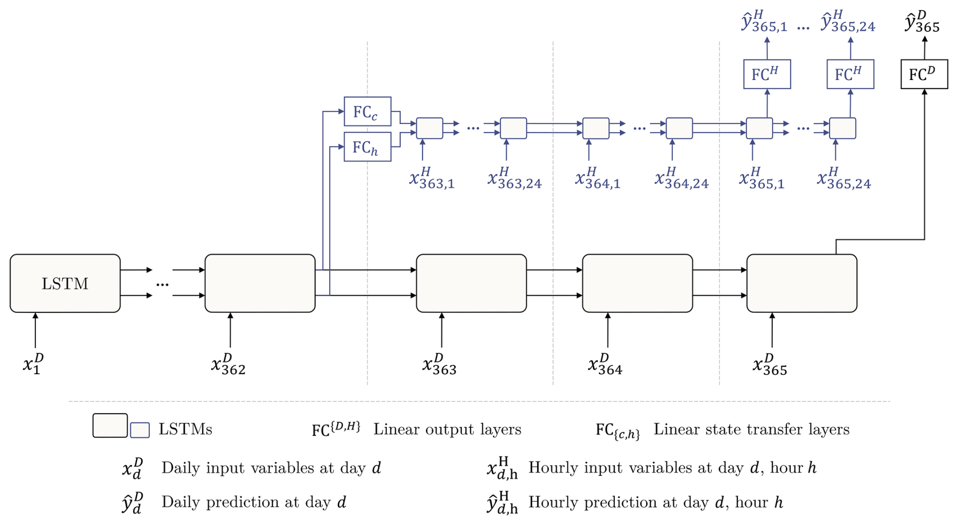
Figure B1 Illustration of the MTS-LSTM architecture that uses one distinct LSTM model per timescale. In the depicted example, the daily and hourly input sequence lengths are T^D=365 and T^H=72 (we chose this value for the sake of a tidy illustration; the benchmarked model uses T^H=336). In the sMTS-LSTM model (i.e. without distinct LSTM branches), FC^C and FC^h are identity functions, and the two branches (including the fully connected output layers FC^H and FC^D) share their model weights. Source: this figure and its description were taken from Gauch et al. (2021).

Appendix C: Additional results

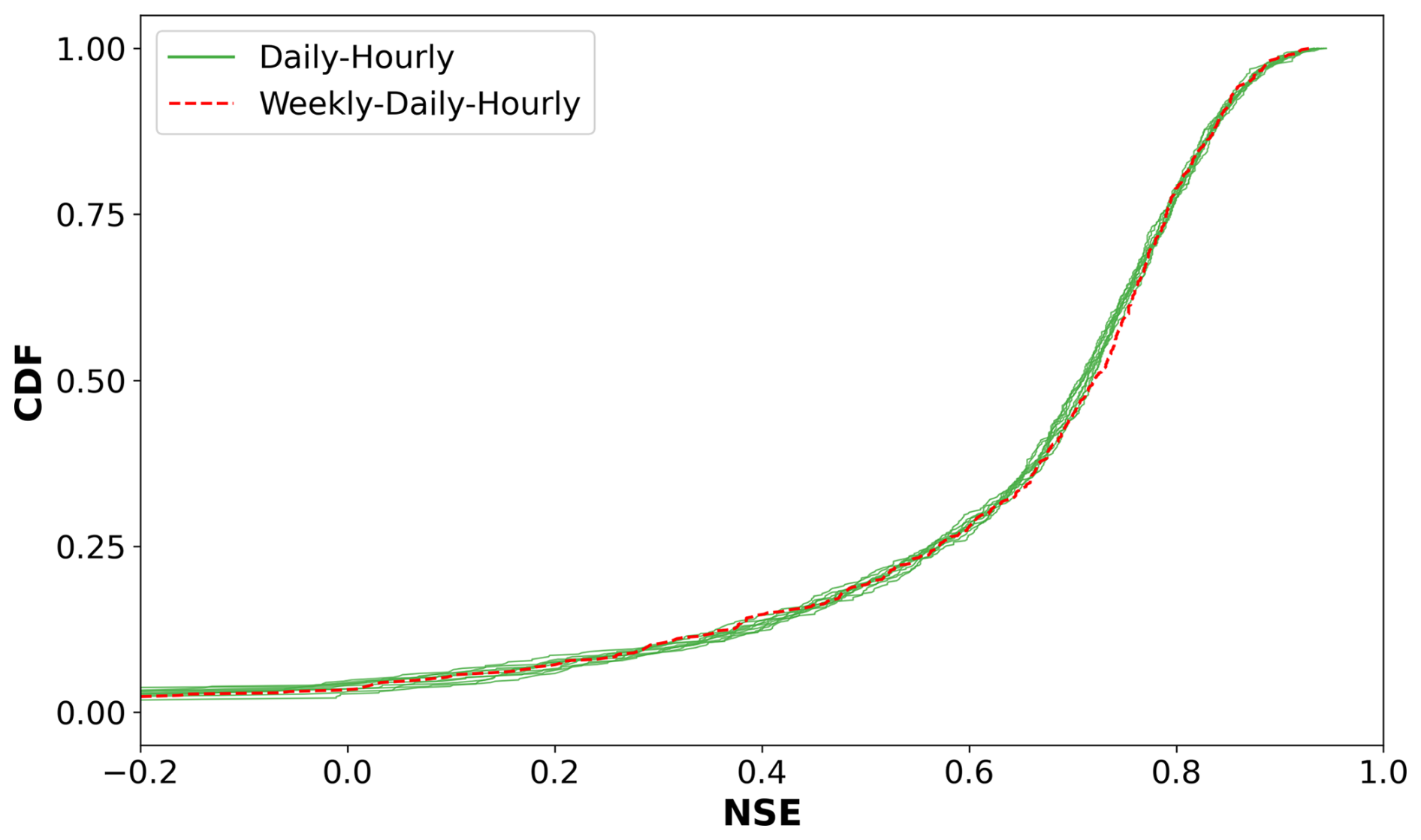
Figure C1 Comparison of cumulative NSE distributions for different frequency sequences. The daily–hourly experiment includes 10 distributions, each corresponding to an ensemble member generated through different random initializations. The average of the 10 median NSE values is 0.71. In contrast, the weekly–daily–hourly experiment consists of a single simulation, yielding a median NSE of 0.72.